Tropical Weierstrass points and Weierstrass weights

Abstract.

In this paper, we study tropical Weierstrass points. These are the analogues for tropical curves of ramification points of line bundles on algebraic curves.

For a divisor on a tropical curve, we associate intrinsic weights to the connected components of the locus of tropical Weierstrass points. This is obtained by analyzing the slopes of rational functions in the complete linear series of the divisor. We prove that for a divisor $D$ of degree $d$ and rank $r$ on a genus $g$ tropical curve, the sum of weights is equal to $d-r+rg$. We establish analogous statements for tropical linear series.

In the case $D$ comes from the tropicalization of a divisor, these weights control the number of Weierstrass points which are tropicalized to each component.

Our results provide answers to open questions originating from the work of Baker on specialization of divisors from curves to graphs.

We conclude with multiple examples which illustrate interesting features appearing in the study of tropical Weierstrass points, and raise several open questions.

1. Overview

Weierstrass points have a rich history in the development of algebraic geometry as they provide an important tool for the study of smooth algebraic curves and their moduli spaces. It is natural to see how their theory can be extended to stable curves, which correspond to boundary points in the Deligne–Mumford compactification $\hbox to0.0pt{\hskip 4.16667pt\leavevmode\hbox{\set@color$\overline{\hbox{}}$}\hss}{\leavevmode\hbox{\set@color$\mathscr{M}$}}_{{g}}$ of the moduli space of genus $g$ curves. One strategy is to take the limit Weierstrass points induced by a one-parameter family $(X_{t})_{t\neq 0}$ of smooth curves degenerating to a stable curve $X_{0}$; there will be $g^{3}-g$ limit Weierstrass points on $X_{0}$ when counted with appropriate weights. However, the limit points generally depend on the chosen family, and a stable curve $X_{0}$ has many possible smoothings corresponding to paths in $\hbox to0.0pt{\hskip 4.16667pt\leavevmode\hbox{\set@color$\overline{\hbox{}}$}\hss}{\leavevmode\hbox{\set@color$\mathscr{M}$}}_{{g}}$ that end at the point representing $X_{0}$.

Tropical geometry provides a new perspective on degeneration methods in algebraic geometry by enriching it with polyhedral geometry. Given the successes of tropical methods in the past two decades in the study of algebraic curves and their moduli spaces, it is natural to ask whether there is a possibility to use tropical geometry in getting insight about the limiting behavior of Weierstrass points on degenerating families of curves. In the tropical perspective, the data of a stable curve $X_{0}$ is replaced by the data of its dual graph. The collection of all stable curves having the same dual graph forms a stratum of $\hbox to0.0pt{\hskip 4.16667pt\leavevmode\hbox{\set@color$\overline{\hbox{}}$}\hss}{\leavevmode\hbox{\set@color$\mathscr{M}$}}_{{g}}$. This gives a correspondence between the strata of $\hbox to0.0pt{\hskip 4.16667pt\leavevmode\hbox{\set@color$\overline{\hbox{}}$}\hss}{\leavevmode\hbox{\set@color$\mathscr{M}$}}_{{g}}$ and the set of stable graphs of genus $g$.

The prototype of what we can expect to address using tropical techniques is the following natural question.

Question 1.1.

Given a stratum of $\hbox to0.0pt{\hskip 4.16667pt\leavevmode\hbox{\set@color$\overline{\hbox{}}$}\hss}{\leavevmode\hbox{\set@color$\mathscr{M}$}}_{{g}}$, and a log-tangent direction of approaching that stratum, what can be said about the limit Weierstrass points of a smooth family $(X_{t})_{t\neq 0}$ degenerating to a stable curve in that stratum along the chosen direction?

The arithmetic geometric version of the above question is the following.

Question 1.2.

Given a smooth proper curve over the field $\mathbb{Q}_{p}$ of $p$-adic numbers with stable reduction lying in a given stratum of $\hbox to0.0pt{\hskip 4.16667pt\leavevmode\hbox{\set@color$\overline{\hbox{}}$}\hss}{\leavevmode\hbox{\set@color$\mathscr{M}$}}_{{g}}$ (over the algebraic closure of the residue field $\mathbb{F}_{p}$), what can be said about the specialization of the Weierstrass points?

Previously, there has been much work making incremental progress on the first question [EH87a, EM02, ES07, Dia85, Ami14, Gen21] and on the second question [Ogg78, LN64, Atk67, AP03, Bak08]; see Section 1.3 for a more thorough discussion.

Our aim in this paper is to provide an answer to the above questions from the point of view of tropical geometry. This is done by introducing new tools which allow us to solve problems on the tropical geometry of curves whose origin goes back to the beginning of the use of tropical methods in the study of algebraic curves.

Our answer to Question 1.1 can be summarized as follows: we can specify how many Weierstrass points degenerate to each component and to each node of a stable curve $X_{0}$ lying in the given stratum. This is done without specifying their precise position within each irreducible component, giving instead a more precise location of those degenerating to a node by specifying their position on the dual metric graph of the family $(X_{t})$. Our result also applies to limits of ramification points of arbitrary line bundles, in addition to the case of the canonical bundle.

Similarly, we answer Question 1.2 by specifying where Weierstrass points specialize when reducing modulo $p$.

These results lead moreover to an effective way of locating the limit Weierstrass points.

In the rest of this introduction, we give an overview of our results.

1.1. Tropical perspective

The central concept studied in this paper is that of tropical Weierstrass points. The definition is based on divisor theory on metric graphs, and we refer to the survey paper [BJ16] and the references there for more details.

Let $\Gamma$ be a metric graph, and let $D$ be a divisor of degree $d$ and rank $r$ on $\Gamma$.

Definition 1.3 (Weierstrass points).

A point $x$ in $\Gamma$ is called a Weierstrass point, or ramification point, for $D$ if there exists an effective divisor $E$ in the linear system of $D$ whose coefficient at $x$ is at least $r+1$. The (tropical) Weierstrass locus of $D$, denoted by $L_{\scaleto{W}{4pt}}(D)$, is the set of all such points in $\Gamma$. ∎

The set $L_{\scaleto{W}{4pt}}(D)$ is a closed subset of $\Gamma$ which can be infinite, in contrast with the classical setting of algebraic curves. In this regard, Baker comments in [Bak08, Remark 4.14], regarding the canonical divisor, that “it is not clear if there is an analogue for metric graphs of the classical fact that the total weight of all Weierstrass points on a smooth curve of genus $g$ is $g^{3}-g$.” More generally, we can ask the following question.

Question 1.4.

Is it possible to associate intrinsic tropical weights to the connected components of $L_{\scaleto{W}{4pt}}(D)$? What is the total sum of weights associated to these components?

The following question is a special case.

Question 1.5.

Assume the locus of Weierstrass points of $D$ is finite. What is the total weight of these points?

Our aim in this paper is to provide answers to the above questions. In order to streamline the presentation which follows, we first discuss our results in the case of non-augmented metric graphs. From the geometric perspective, this corresponds to the situation of a totally degenerate stable curve, that is, a stable curve whose irreducible components are all projective lines. This is the same as requiring that the arithmetic genus of the stable curve is equal to the genus of the dual graph. We have an analogue of these statements in the general setting, see the discussion which follows below.

In order to solve Question 1.4, we make the following definition.

Definition 1.6 (Intrinsic Weierstrass weight of a connected component).

Let $D$ be a divisor of rank $r$, and let $C$ be a connected component of the Weierstrass locus $L_{\scaleto{W}{4pt}}(D)$. We define the tropical Weierstrass weight of $C$ as

(1) $$\mu_{\scaleto{W}{4pt}}(C;D)\coloneqq\deg\left({D}\raisebox{-1.0pt}{$|$}_{C}\right)+\left(g(C)-1\right)r-\sum_{\nu\in\partial^{{}^{\scaleto{\mathrm{out}}{3pt}}}C}s_{0}^{\nu}(D)$$

where

• $\deg\left({D}\raisebox{-1.0pt}{$|$}_{C}\right)$ is the total degree of $D$ in $C$, defined by $\deg\left({D}\raisebox{-1.0pt}{$|$}_{C}\right)=\sum_{x\in C}D(x)$;

• $g(C)$ is the genus of $C$, i.e., its first Betti number $\dim H_{1}(C,\mathbb{R})$;

• $\partial^{{}^{\scaleto{\mathrm{out}}{3pt}}}C$ is the set of outgoing unit tangent directions from $C$; and

• $s_{0}^{\nu}(D)$ is the minimum slope at $x$ along tangent direction $\nu$ of any rational function $f$ on $\Gamma$ with $\mathrm{div}(f)+D\geq 0$.

We abbreviate $\mu_{\scaleto{W}{4pt}}(C;D)$ simply as $\mu_{\scaleto{W}{4pt}}(C)$ if $D$ is understood from the context. ∎

Although it is not straightforward from the definition, we will show in Theorem 3.6 that the tropical Weierstrass weight of any component is positive. Note as well that a connected component of $L_{\scaleto{W}{4pt}}(D)$ is always a metric subgraph of $\Gamma$, see Proposition 3.1.

We say that $D$ is Weierstrass finite or simply W-finite if the tropical Weierstrass locus $L_{\scaleto{W}{4pt}}(D)$ has finite cardinality. In this case, connected components of $L_{\scaleto{W}{4pt}}(D)$ are isolated points in $\Gamma$, and we define the tropical Weierstrass divisor $W(D)$ as the effective divisor

$$W(D)\coloneqq\sum_{x\in L_{\scaleto{W}{4pt}}(D)}\mu_{\scaleto{W}{4pt}}(x)\,(x)$$

where $\mu_{\scaleto{W}{4pt}}(x)\coloneqq\mu_{\scaleto{W}{4pt}}(\{x\})$. The support $|W(D)|$ of the tropical Weierstrass divisor is exactly the tropical Weierstrass locus $L_{\scaleto{W}{4pt}}(D)$. The tropical Weierstrass weight of $x$ can be identified as $\mu_{\scaleto{W}{4pt}}(x)=D_{x}(x)-r$, with $D_{x}$ denoting the unique $x$-reduced divisor in the linear system of $D$, see Remark 3.3.

This gives the following geometric meaning to the Weierstrass weights, in the spirit of the classical definition on algebraic curves. The coefficient of the reduced divisor at a point $x\in\Gamma$ corresponds precisely to the maximum order of vanishing at $x$ of any global section of the line bundle $\mathcal{O}(D)$ defined by the divisor. The Weierstrass weight of the point $x$ is thus obtained by comparing this quantity to $r$, which would be the expected minimum value, over points $y\in\Gamma$, of the largest order of vanishing of global sections at $y$. (Note, however, that $r$ is not always equal to the actual minimum largest order of vanishing, as examples in Section 6.5 show.) That being said, the definition differs from the algebraic setting, where we need to take into account all the orders of vanishing of global sections of the line bundle at a given point (and then compare them with the standard sequence, the one obtained for a point in general position on the curve).

The following theorem answers Questions 1.4 and 1.5, and is proved in Section 3.3.

Theorem 1.7 (Total weight of the Weierstrass locus).

Let $\Gamma$ be a metric graph of genus $g$, and let $D$ be an effective divisor of degree $d$ and rank $r$ on $\Gamma$. Then, the total sum of weights of the connected components of $L_{\scaleto{W}{4pt}}(D)$ is equal to $d-r+rg$. In particular, if $D$ is W-finite, then we have $\deg(W(D))=d-r+rg$.

The proof of this theorem will imply in particular the following result, proved in Section 3.4.

Theorem 1.8.

If the rank $r$ of $D$ is at least one, then every cycle in $\Gamma$ intersects the tropical Weierstrass locus $L_{\scaleto{W}{4pt}}(D)$. In particular, if $\Gamma$ has genus at least two, then every cycle intersects the Weierstrass locus of the canonical divisor $K$.

In [Bak08], Baker proves that the tropical Weierstrass locus of the canonical divisor is nonempty if $\Gamma$ has genus at least two. This earlier tropical result is obtained as a consequence of the analogous algebraic statement, using the specialization lemma. In contrast, our theorem above states that tropical Weierstrass points obey a stronger “local” existence condition, which has seemingly no algebraic analogue. In the case that the canonical divisor of $\Gamma$ is W-finite, our result implies that for an arbitrary family $(X_{t})_{t\neq 0}$ of smooth curves tropicalizing to $\Gamma$, every cycle in $\Gamma$ contains a limit Weierstrass point of the family.

To prove Theorem 1.7, we will show that in fact (1) defines a consistent notion of Weierstrass weight when applied to any connected, closed subset of $\Gamma$ whose boundary points are not in the interior of $L_{\scaleto{W}{4pt}}(D)$; see Theorem 3.9. To do so, we retrieve information about the slopes of rational functions in the linear series $\operatorname{Rat}(D)$ along tangent directions in $\Gamma$. We have the following description, proved in Section 2.

Theorem 1.9.

Let $D$ be a divisor of rank $r$ on $\Gamma$. We take a model for $\Gamma$ whose vertex set contains the support of $D$. Let $x\in\Gamma$ be a point and $\nu\in\mathrm{T}_{x}(\Gamma)$ be a tangent direction.

1. If the open interval $(x,x+\varepsilon\nu)$ is disjoint from $L_{\scaleto{W}{4pt}}(D)$ for some $\varepsilon>0$, then the set of slopes $\{\mathrm{sl}_{\nu}f(x):f\in\operatorname{Rat}(D)\}$ consists of $r+1$ consecutive integers $\{s^{\nu}_{0},s^{\nu}_{0}+1,\dots,s^{\nu}_{0}+r\}$.

2. If the open interval $(x,x+\varepsilon\nu)$ is contained in $L_{\scaleto{W}{4pt}}(D)$, then the set of slopes $\{\mathrm{sl}_{\nu}f(x):f\in\operatorname{Rat}(D)\}$ is a set of consecutive integers of size at least $r+2$.

1.2. Tropicalization and extensions

We further justify our definition of weights by making a precise link to tropicalizations of Weierstrass points on algebraic curves.

Suppose that $\Gamma$ and $D$ come from geometry; that is, let $X$ be a smooth proper curve of genus $g$ over an algebraically closed non-Archimedean field $\mathbb{K}$ of characteristic zero with a non-trivial valuation and a residue field of arbitrary characteristic. Let $\mathcal{L}=\mathcal{O}(\mathcal{D})$ be a line bundle of degree $d$ on $X$. Assume that $\Gamma$ is a skeleton of the Berkovich analytification $X^{\operatorname{an}}$ of $X$. Denote by $\tau$ the tropicalization map from $X$ to $\Gamma$, and suppose that $D=\tau_{*}\left(\mathcal{D}\right)$ is the tropicalization of $\mathcal{D}$ on $\Gamma$ where $\tau_{*}\colon\operatorname{Div}(X)\to\operatorname{Div}(\Gamma)$ the induced map on divisors.

Denote by $\mathcal{W}(\mathcal{D})$ the Weierstrass divisor of $\mathcal{D}$ on $X$, and by $\tau_{*}\left(\mathcal{W}(\mathcal{D})\right)$ its tropicalization on $\Gamma$. The following result, proved in Section 5.4, uses the notion of $L_{\scaleto{W}{4pt}}(D)$-measurable set, for which the connected components of $L_{\scaleto{W}{4pt}}(D)$ form the atoms, and the natural counting measure $\hat{\mu}_{\scaleto{W}{4pt}}$ on such sets, induced by Weierstrass weights (see Section 3.3 for more details).

Theorem 1.10 (Algebraic versus tropical Weierstrass weights).

Assume that $D$ and $\mathcal{D}$ have the same rank, and let $A\subset\Gamma$ be a closed, connected subset which is $L_{\scaleto{W}{4pt}}(D)$-measurable. Then, the total weight of Weierstrass points of $\mathcal{W}(\mathcal{D})$ tropicalizing to points in $A$ is precisely $(r+1)\,\hat{\mu}_{\scaleto{W}{4pt}}(A;D)$; that is,

$$\deg\left({\mathcal{W}(\mathcal{D})}\raisebox{-1.0pt}{$|$}_{\tau^{-1}(A)}\right)=(r+1)\left(\deg\left({D}\raisebox{-1.0pt}{$|$}_{A}\right)+r\left(g(A)-1\right)-\sum_{\nu\in\partial^{{}^{\scaleto{\mathrm{out}}{3pt}}}A}s_{0}^{\nu}(D)\right).$$

In particular, if $D$ is W-finite, then we have the equality

$$\tau_{*}\left(\mathcal{W}(\mathcal{D})\right)=(r+1)\,W(\tau_{*}\left(\mathcal{D}\right)).$$

This statement, which involves the metric of $\Gamma$ in a crucial way, gives an essentially complete description of the behavior of Weierstrass points in the tropical limit. In particular, if the limit divisor is W-finite, then for every family $(X_{t})_{t\neq 0}$ of smooth proper curves approaching a stable curve with dual metric graph $\Gamma$, the limit Weierstrass points are precisely described by the tropical Weierstrass divisor. This rigidity type theorem on the limiting behavior of Weierstras points allows us to give a precise count of the number of Weierstrass points going to the nodes or to the smooth parts of a limit stable curve $X_{0}$ on the given stratum of $\hbox to0.0pt{\hskip 4.16667pt\leavevmode\hbox{\set@color$\overline{\hbox{}}$}\hss}{\leavevmode\hbox{\set@color$\mathscr{M}$}}_{{g}}$ along the given log-tangent direction from which the family $(X_{t})_{t\neq 0}$ approaches $X_{0}$. Moreover, as a special case, the theorem also applies in the arithmetic geometric context in which the curve $X$ is defined over a local field. As we will show in Section 5.4, this theorem holds as well over a field $\mathbb{K}$ of positive characteristic provided that the gap sequence of $\mathcal{L}$, defined as the sequence of orders of vanishing of the global sections of $\mathcal{L}$ at a general point of $X$, is the standard sequence $0,1,\dots,r$. (In this case, $\mathcal{L}$ is called classical [Lak81, Nee84].)

We provide natural extensions and refinements of the above results to the setting of augmented metric graphs, which, from the degeneration perspective, corresponds to the more general situation where the limit stable curve has irreducible components of possibly positive genus. Since a given vertex of positive genus hides information about the geometry of the component, it turns out that there will be an ambiguity when talking about the Weierstrass locus of a divisor $D$. In fact, the right setup in this context is a divisor $D$ endowed with the data of a closed sub-semimodule $M$ of $\operatorname{Rat}(D)$, which plays the role of a (not necessarily complete) linear series on the augmented metric graph.

In this regard, first, we use the weights defined in Definition 1.6 with a relevant notion of divisorial rank associated to the sub-semimodule which we further modify by including the data of the genus function. We get Theorem 4.12, which provides a global count of weights in this setting.

To the question of whether it is still possible to associate a natural Weierstrass locus to a divisor in the augmented setting, we provide an answer by introducing two special classes of semimodules, the generic semimodule associated to any divisor (see Section 4.2), and the canonical semimodule associated to the canonical divisor on an augmented metric graph (see Section 4.3). Both of them require some level of genericity, which we properly justify in Section 4.4 using the framework of metrized complexes.

The case of the canonical divisor on an augmented metric graph is particularly interesting as it reveals new facets of divisor theory in the augmented setting. We associate a canonical linear series to any augmented metric graph, show that it has the appropriate rank, and study its Weierstrass locus. To justify the definition and prove these results, we use the setting of metrized complexes and their divisor theory from [AB15]. Using that framework, we show that the canonical linear series on an augmented metric graph is the tropical part of the canonical linear series on any metrized complex with that underlying augmented metric graph, provided that the markings associated to edges on the curves of the metrized complex are in general position. It is interesting to note that this is the assumption made in the works by Esteves and coauthors [EM02, ES07], and our results here complement these works by developing the tropical part of the story in greater generality.

As we show in Theorem 5.5, the statement of Theorem 1.10 remains valid in these settings (when including the genera of points of $A$ on the right-hand side of the stated equality). The following theorem is a direct application of our results on Weierstrass weights for an augmented metric graph. We use the setting of tropicalization preceding Theorem 1.10.

Theorem 1.11.

Suppose $\mathcal{D}$ is a divisor on an algebraic curve $X$ over an algebraically closed non-Archimedean field $\mathbb{K}$ of characteristic zero with a non-trivial valuation and a residue field of arbitrary characteristic. Let $(\Gamma,\mathfrak{g})$ be an (augmented) skeleton of $X^{\operatorname{an}}$. Let $H$ be a vector space of global sections of $\mathcal{O}(\mathcal{D})$ of rank $r$ and denote by $\mathcal{W}(H)$ the Weierstrass divisor of $H$. Let $M$ be the tropicalization of $H$. Then, for any connected, closed subset $A\subset\Gamma$ which is $L_{\scaleto{W}{4pt}}(M,\mathfrak{g})$-measurable, we have the bound

$$\deg\left({\mathcal{W}(H)}\raisebox{-1.0pt}{$|$}_{\tau^{-1}(A)}\right)\geq\left(r^{2}+r\right)\left(g(A)+\sum_{x\in A}\mathfrak{g}(x)\right).$$

The proof of this theorem will be given in Section 5.4. As in the case of Theorem 1.10, the statement holds as well over a field $\mathbb{K}$ of positive characteristic provided the gap sequence of $H$ is the standard sequence.

In the case $L_{\scaleto{W}{4pt}}(M,\mathfrak{g})$ is finite, this inequality holds for any closed subset $A\subset\Gamma$. In particular, we have the following application to stable curves: suppose $X_{0}$ is a stable curve with dual augmented graph $(G,\mathfrak{g})$, and suppose $(X_{t})$ is a family degenerating to $X_{0}$ with tropicalization $(\Gamma,\mathfrak{g})$. If the locus of canonical Weierstrass points of $(\Gamma,\mathfrak{g})$ is finite, then for every connected subgraph $A$ of $G$, the number of limit Weierstrass points lying on components and nodes of $X_{0}$, which correspond to vertices and edges of $A$, respectively, is at least $(g^{2}-g)\left(g(A)+\sum_{v\in A}\mathfrak{g}(v)\right)$.

The recent works [AG22] and [JP22] develop a combinatorial theory of (limit) linear series. In Section 5, we associate to any such linear series a divisor of Weierstrass points, and connect it with the Weierstrass locus associated to linear series in the preceding sections. The definition of this combinatorial Weierstrass divisor takes into account the higher orders of vanishing of the combinatorial limit linear series, and is closer to the spirit of the algebraic definition of Weierstrass weights on curves.

Then, we provide the proof of Theorem 1.10 and its extensions to the augmented and incomplete setting. Finally, using combinatorial Weierstrass divisors, we formulate obstructions to the realizability of combinatorial limit linear series.

1.3. Previous work

For an extensive and informative survey describing the history and applications of Weierstrass points, starting with Weierstrass and Hürwitz [Wei67, Hur92] in the 1800s, see Del Centina [DC08]. The study of Weierstrass points on stable curves was initiated by Eisenbud and Harris [EH87a], who proved results on nodal curves of compact type, i.e., curves whose dual graph is a tree. This work served as an application of their newly-developed theory of limit linear series [EH86]. They moreover raised the question of constructing a moduli space parametrizing all possible limit Weierstrass divisors of a given stable curve, a problem which has been widely open since then.

Moving beyond stable curves of compact type, Lax [Lax87b] studied Weierstrass points on stable curves which consist of one rational component with nodes; in this case, the dual graph is a single vertex with self-loops. (The term tree-like is used in the literature to describe curves whose dual graph consists of a tree after removing self-loops.) A further breakthrough came with Esteves–Medeiros [EM02] who worked with stable curves with two components, i.e., curves whose dual graph is a dipole graph. (We refer to Section 6.8 for a discussion of our results applied to dipole graphs and the connection to [EM02].) Esteves–Salyehan [ES07] studied further cases, including when the dual graph is a complete graph. Cumino–Esteves–Gatto [CEG08] studied limits of special Weierstrass points on certain stable curves, i.e., Weierstrass points with weight at least two. The problem of describing limits of Weierstrass points in a given one-parameter family is addressed in [Est98, Ami14].

Other works have attempted to treat the case of irreducible Gorenstein curves and the distribution of Weierstrass points on them [Lax87a, LF90, LW90, GL93, dCS94, GL95, GL96, BG95, Est96].

The study of Weierstrass points from a tropical perspective was initiated by Baker [Bak08, Section 4]. Baker defines Weierstrass points for graphs and metric graphs, and uses his Specialization Lemma [Bak08, Lemma 2.8] to prove an essential compatibility with Weierstrass points on stable curves. Baker motivates his theory of Weierstrass points on graphs with several results from the arithmetic geometry of modular curves, in particular, as a way to decide whether certain cusps are Weierstrass points, c.f. [Ogg78, LN64, Atk67, AP03]. The question of how to determine limits of Weierstrass points in one-parameter families of Riemann surfaces is settled in [Ami14] if we take into account non-Archimedean data associated to the family. Although the tropical Weierstrass locus may be infinite, [Ric18] provides conditions in which it is generically finite and computes the cardinality of the Weierstrass locus under this genericity assumption. The way Weierstrass points of line bundles get distributed on (limit) tropical curves is also studied in [Ami14, Ric18]. For an extended discussion of how divisor theory on graphs is connected to the degeneration of smooth curves to nodal curves, with various applications, see the survey by Baker–Jensen [BJ16], in particular Section 12. Degeneration of Weierstrass points is also discussed in Lax [Lax87c], in non-tropical language.

Weierstrass points have appeared in other interesting work on moduli spaces of curves. Arbarello [Arb74] studied subvarieties of the moduli space of curves cut out by Weierstrass points; further results were found in Lax [Lax75] and Diaz [Dia85]. Eisenbud–Harris [EH87b] showed that the moduli space of curves has positive Kodaira dimension, using loci of Weierstrass points as part of their argument. Cukierman [Cuk89] found the coefficients for the Weierstrass locus in the universal curve $\mathscr{C}_{{{g}}}$ of genus $g$, in a standard basis for the Picard group of $\mathscr{C}_{{{g}}}$. Cukierman–Fong [CF91] proved similar results for higher Weierstrass points, i.e., Weierstrass points of the pluricanonical bundle $\omega^{\otimes k}$.

1.4. Organization of the text

The paper is organized as follows. We first treat the case of non-augmented metric graphs, and then provide refinements. This choice has the advantage of making the presentation less technical, and we hope this will add to readability.

We define slope sets and prove Theorem 1.9 in Section 2.

In Section 3, we study Weierstrass weights and the Weierstrass measure they define on a metric graph. We state and prove Theorem 3.9, which provides a description of the Weierstrass measure using the slopes, from which we deduce Theorem 1.7 and other interesting consequences. This section contains the proof of positivity of Weierstrass weights as well, and a discussion of the case of combinatorial graphs. The case of the canonical Weierstrass locus on non-augmented metric graphs is treated in Section 3.7.

Section 4 provides several refinements and generalizations of the previous sections. The setting is extended in two ways. First, complete linear series $\operatorname{Rat}(D)$ are replaced with incomplete linear series, by taking closed sub-semimodules of $\operatorname{Rat}(D)$. Second, metric graphs are replaced with augmented metric graphs. We provide justification for our definitions in the augmented setting and provide the corresponding generalizations of Theorem 3.9 on the Weierstrass measure and of Theorem 1.7.

In Section 5, we explain how to associate Weierstrass divisors to combinatorial limit linear series arising in the recent work [AG22]. This is particularly interesting in the case where the locus of Weierstrass points associated to the underlying divisor becomes infinite after forgetting the slopes underlying the definition of limit linear series in [AG22]. We show the compatibility of the definitions appearing in this section with the previous ones.

Using the above materials, we establish a precise link between the tropical Weierstrass divisors with tropicalizations of Weierstrass divisors on smooth curves. This includes the proof of Theorem 1.10, and its generalizations.

In the last two Sections 6 and 7, we provide several examples with the aim of clarifying the concepts introduced in previous sections, and discuss other interesting results related to them. We also raise several open questions.

Acknowledgments

This material is based upon research supported by the Transatlantic Research Partnership of the Embassy of France in the United States and the FACE Foundation. We thank them, as well as the Cultural Services of the French Embassy in the U.S., and the administrations of the CNRS and the University of Washington at Seattle, for support.

O. A. thanks Math+, the Berlin Mathematics Research Center and TU Berlin, where this research was carried out. L. G. thanks the Mathematical Foundation Jacques Hadamard (FMJH) for financial support.

1.5. Basic notations

A (combinatorial) graph $G=(V,E)$ is defined by a set of vertices $V$ and a set of edges $E$ between certain vertices. In the current paper, graphs will always be taken to be finite and connected. Moreover, they will allow loops and multiple edges.

A metric graph is a compact, connected metric space $\Gamma$ verifying the following properties:

1. For every point $x\in\Gamma$, there exist a positive integer $n_{x}$ and a real number $r_{x}>0$ such that the $r_{x}$-neighborhood of $x$ is isometric to the star of radius $r_{x}$ with $n_{x}$ branches.

2. The metric on $\Gamma$ is given by the path metric, i.e., for points $x$ and $y$ in $\Gamma$, the distance between $x$ and $y$ is the infimum (in fact minimum) length of any path from $x$ to $y$.

The integer $n_{x}$ above is called the valence of $x$ and is denoted by $\operatorname{val}(x)$.

Given a graph $G=(V,E)$ and a length function $\ell\colon E\to(0,+\infty)$ assigning to every edge of $G$ a positive length, we can build from this data a metric graph $\Gamma$ by glueing a closed interval of length $\ell(e)$ between the two endpoints of the edge $e$, for every $e\in E$, and endowing $\Gamma$ with the path metric. The space $\Gamma$ is then called the geometric realization of the pair $(G,\ell)$.

A model of a metric graph $\Gamma$ is a pair $(G,\ell)$ consisting of a graph $G=(V,E)$ and a length function $\ell\colon E\to(0,+\infty)$ such that $\Gamma$ is isometric to the geometric realization of $(G,\ell)$. By an abuse of notation, we also call $G$ a model of $\Gamma$.

For a metric graph $\Gamma$ and a point $x\in\Gamma$, the tangent space $\mathrm{T}_{x}(\Gamma)$ is defined as the set of all unit outgoing tangent vectors to $\Gamma$ at $x$. This is a finite set of cardinality $\operatorname{val}(x)$. If $G=(V,E)$ is a loopless model for $\Gamma$ such that $x\in V$, then $\mathrm{T}_{x}(\Gamma)$ is in one-to-one correspondence with the edges of $G$ incident to $x$. Through this natural bijection, a tangent direction $\nu$ is said to be supported by the corresponding edge $e\in E$.

Each edge $e$ supports two tangent directions, which belong to either endpoint of $e$, respectively. If $\nu$ is one of those tangent directions, the opposite direction is denoted by $\overline{\nu}$. For $\nu\in\mathrm{T}(\Gamma)$, we denote by $x_{\nu}$ the point $x$ with $\nu\in\mathrm{T}_{x}(\Gamma)$.

In this paper, all the semimodules will be assumed to be nonempty.

2. Slope sets

In this section, we prove Theorem 1.9. We first recall some terminology for divisors and functions on metric graphs.

Given a metric graph $\Gamma$, let $\operatorname{Div}(\Gamma)$ denote the group of divisors of $\Gamma$, which is the free abelian group generated by points $x\in\Gamma$. Let $\operatorname{Rat}(\Gamma)$ denote the set of real-valued piecewise linear functions on $\Gamma$ whose slopes are all integers. Given a function $f\in\operatorname{Rat}(\Gamma)$, let $\mathrm{div}(f)$ denote the principal divisor of $f$, defined as

$$\mathrm{div}(f)\coloneqq\sum_{x\in\Gamma}a_{x}(x)\qquad\text{where}\qquad a_{x}=-\sum_{\nu\in\mathrm{T}_{x}(\Gamma)}\mathrm{sl}_{\nu}f(x).$$

Let $D$ be a divisor of rank $r$ on $\Gamma$. Let $\operatorname{Rat}(D)$ denote the set of rational functions in the complete linear series of $D$ defined as

$$\operatorname{Rat}(D)\coloneqq\{f\in\operatorname{Rat}(\Gamma):D+\mathrm{div}(f)\geq 0\}.$$

Given a point $x\in D$, there is a unique representative $f_{x}$ of the linear series of $D$ defined by

$$f_{x}\coloneqq\min_{\begin{subarray}{c}f\in\operatorname{Rat}(D)\\ f(x)=0\end{subarray}}f.$$

The corresponding divisor $D+\mathrm{div}(f_{x})$, denoted by $D_{x}$, is the (unique) $x$-reduced divisor linearly equivalent to $D$. This statement is a consequence of the maximum principle, see e.g. [BS13, Lemma 4.11].

Definition 2.1 (Slope sets and minimum slopes).

Let $D$ be an effective divisor on $\Gamma$. Given a point $x\in\Gamma$ and a tangent direction $\nu\in\mathrm{T}_{x}(\Gamma)$, let $\mathfrak{S}^{\nu}(D)$ denote the slope set

$$\mathfrak{S}^{\nu}(D)\coloneqq\{\mathrm{sl}_{\nu}f(x):f\in\operatorname{Rat}(D)\}.$$

Let $s_{0}^{\nu}(D)$ denote the minimum slope in the slope set $\mathfrak{S}^{\nu}(D)$, i.e.,

$$s_{0}^{\nu}(D)\coloneqq\min\{\mathrm{sl}_{\nu}f(x):f\in\operatorname{Rat}(D)\}.$$

When the divisor $D$ is clear from context, we will simply use $s_{0}^{\nu}$ to denote $s_{0}^{\nu}(D)$. ∎

Lemma 2.2.

Suppose $D$ is a divisor of rank $r$. Then, for every $x\in\Gamma$ and every $\nu\in\mathrm{T}_{x}(\Gamma)$, there are at least $r+1$ integers in the set of slopes $\{\mathrm{sl}_{\nu}f(x):f\in\operatorname{Rat}(D)\}$.

Proof.

Let $x_{1},\dots,x_{r}$ be a set of distinct points in the branch incident to $x$ in the direction of $\nu$ sufficiently close to $x$. There exists a function $f\in\operatorname{Rat}(D)$ such that

$$D+\mathrm{div}(f)\geq(x_{1})+\dots+(x_{r}).$$

The function $f$ changes slope at the points $x_{1},\dots,x_{r}$. Each of the slopes taken at $x_{j}$ in the direction of $\nu$ can be obtained as the slope of a function in $\operatorname{Rat}(D)$ at $x$ along $\nu$. ∎

The minimum slope $s^{\nu}_{0}(D)$ is related to the reduced divisor $D_{x}$ at $x$.

Lemma 2.3.

Let $D$ be an effective divisor on $\Gamma$, and $x$ a point of $\Gamma$. Let $D_{x}$ be the $x$-reduced divisor linearly equivalent to $D$.

1. Let $f_{x}$ be the above defined rational function satisfying $\mathrm{div}(f_{x})+D=D_{x}$, then, for any outgoing tangent vector $\nu\in\mathrm{T}_{x}(\Gamma)$,

   $$s_{0}^{\nu}(D)=\mathrm{sl}_{\nu}f_{x}(x).$$

2. The coefficient of $D_{x}$ at $x$ satisfies

   $$D_{x}(x)=D(x)-\sum_{\nu\in\mathrm{T}_{x}(\Gamma)}s_{0}^{\nu}(D).$$

Proof.

The first result is obtained by observing that $f_{x}=\min h$ for $h\in\operatorname{Rat}(D)$ verifying $h(x)=0$. The second result is a direct consequence of (a) and the definition of the principal divisor $\mathrm{div}(f_{x})$. ∎

We now turn to the proof of Theorem 1.9. Let $D$ be a divisor of rank $r$ on $\Gamma$. Recall (Definition 1.3) that the Weierstrass locus of $D$, denoted by $L_{\scaleto{W}{4pt}}(D)$, is the subset of $\Gamma$ formed by the points $x$ such that there exists en effective divisor $E\sim D$ with $E(x)\geq r+1$. Equivalently, $L_{\scaleto{W}{4pt}}(D)$ is defined in terms of reduced divisors as

$$L_{\scaleto{W}{4pt}}(D)=\{x\in\Gamma:D_{x}(x)>r\},$$

where $D_{x}$ denotes the $x$-reduced divisor linearly equivalent to $D$.

Proof of Theorem 1.9.

We first assume that the open interval $(x,x+\varepsilon\nu)$ is disjoint from $L_{\scaleto{W}{4pt}}(D)$. Along the branch incident to $x$ in the direction of $\nu$, there is a small segment on which $s^{\nu}_{0}$ is the slope of a function in $\operatorname{Rat}(D)$, and it is the smallest slope taken by a function of $\operatorname{Rat}(D)$ on this segment. If a slope of $s^{\nu}_{0}+r+1$ or larger is achieved at $x$, then, again on a small segment, it will be achieved at any point of that segment. This means that on the interior of this segment, the two minimum outgoing slopes at every point are $s^{\nu}_{0}$ and $-s^{\nu}_{0}-s^{\prime}$ with $s^{\prime}\geq r+1$. Therefore, by Lemma 2.3, we infer that on the interior of this segment, the reduced divisor at each point has coefficient at least $r+1$. This contradicts the assumption that a neighborhood $(x,x+\varepsilon\nu)$ is disjoint from $L_{\scaleto{W}{4pt}}(D)$, and shows that the highest possible slope is $s^{\nu}_{0}+r$. Combining this with Lemma 2.2, the slopes achieved at $x$ along $\nu$ must be precisely $s^{\nu}_{0},s^{\nu}_{0}+1,\ldots,s^{\nu}_{0}+r$. This proves (a).

We now assume that $(x,x+\varepsilon\nu)\subset L_{\scaleto{W}{4pt}}(D)$ and that $\varepsilon$ is small enough so that the set of slopes of functions of $\operatorname{Rat}(D)$ along $\nu$ is constant on this interval. By Lemma 2.3, this means that on the interior of a small segment starting at $x$, the two minimum outgoing slopes at every point are $s^{\nu}_{0}$ and $-s^{\nu}_{0}-s^{\prime}$ with $s^{\prime}\geq r+1$. Therefore, close to $x$, a slope of at least $s^{\nu}_{0}+r+1$ is achieved by a function in $\operatorname{Rat}(D)$. To prove (b), it is thus sufficient to show that the set of slopes $\mathrm{sl}_{\nu}f(x)$ of functions $f\in\operatorname{Rat}(D)$ is always made up of consecutive integers. Take $s_{1}<s_{2}<s_{3}$ to be three integers, and suppose that for $i\in\{1,3\}$ there exists a function $f_{i}\in\operatorname{Rat}(D)$ such that $\mathrm{sl}_{\nu}f_{i}(x)=s_{i}$. Using $f_{1}$, $f_{3}$ and tropical operations, it is easy to construct a function $f$ taking slopes $s_{3}$ and then $s_{1}$ away from $x$, changing slope at a point we denote by $y$ (see Figure 1). We can then “chop up” the graph of $f$ to construct a function $g$ equal to $f$ everywhere except on a small interval around $y$ where it takes slope $s_{2}$. Since $(x,x+\varepsilon\nu)$ is disjoint from the support of $D$, $g$ still belongs to $\operatorname{Rat}(D)$. The assumption made on $\varepsilon$ at the beginning ensures that in fact there exists a function $f_{2}\in\operatorname{Rat}(D)$ taking slope $s_{2}$ at $x$ along $\nu$, which concludes the argument. ∎

Figure 1. Construction of the functions $f$ and $g$ using functions $f_{1}$ and $f_{3}$ taking slopes $s_{1}<s_{3}$.

Remark 2.4.

In particular, note that along a given unit tangent vector $\nu$ attached to a point $x$, the slopes $\mathrm{sl}_{\nu}f(x)$ for $x\in\operatorname{Rat}(D)$ always form a set of consecutive integers. Moreover, if $t$ is a positive integer such that for every $x\in e$, for $e$ an edge of some model of $\Gamma$, the $x$-reduced divisor $D_{x}$ satisfies $D_{x}\geq t\,(x)$, then for any $x\in\mathring{e}$, the set of slopes $\{\mathrm{sl}_{\nu}f(x):f\in\operatorname{Rat}(D)\}$ contains at least $t+1$ consecutive integers. This claim is analogous to [Ami13, Theorem 14] and is proved using Theorem 3 of the same paper, which gives a concrete description of the variations of the reduced divisor $D_{x}$ with respect to $x$. See also [AG22, Section 6.6]. ∎

For future use, we note the following generalization of part (b) of Lemma 2.3.

Proposition 2.5.

Suppose $D$ is a divisor of rank $r$. Then, for any closed, connected subset $A\subset\Gamma$, we have

$$\deg\left({D}\raisebox{-1.0pt}{$|$}_{A}\right)-\sum_{\nu\in\partial^{{}^{\scaleto{\mathrm{out}}{3pt}}}A}s_{0}^{\nu}(D)\geq r.$$

Proof.

Let $E$ be an effective divisor of degree $r$, with support contained in $A$. Since $D$ has rank $r$, there exists a function $f\in\operatorname{Rat}(D)$ such that $D+\mathrm{div}(f)\geq E$. Evaluating the respective degrees restricted to $A$ yields

$$\deg\left({D}\raisebox{-1.0pt}{$|$}_{A}\right)-\sum_{\nu\in\partial^{{}^{\scaleto{\mathrm{out}}{3pt}}}A}\mathrm{sl}_{\nu}f(x_{\nu})\quad\geq\quad\deg\left({E}\raisebox{-1.0pt}{$|$}_{A}\right)=r,$$

where, we recall, $x_{\nu}$ is the point $x$ of $\Gamma$ with $\nu\in\mathrm{T}_{x}(\Gamma)$. By definition of the minimum slope $s_{0}^{\nu}(D)$, we have $s_{0}^{\nu}(D)\leq\mathrm{sl}_{\nu}f(x_{\nu})$ for each $\nu\in\partial^{{}^{\scaleto{\mathrm{out}}{3pt}}}A$, so the result follows. ∎

3. Weierstrass weights

Using the structure of slope sets in $\operatorname{Rat}(D)$, we prove Theorem 1.7, which will follow from the more general Theorem 3.9.

3.1. Definition of weights and basic properties of the Weierstrass locus

We start by establishing basic properties of Weierstrass loci. The Weierstrass locus $L_{\scaleto{W}{4pt}}(D)$ is defined as the set of points $x$ in $\Gamma$ such that there exists an effective divisor $E$ in the linear system of $D$ whose coefficient at $x$ is at least $r+1$. This is equivalent to requiring that $D_{x}(x)\geq r+1$. Let us now recall Definition 1.6 from the introduction. Given a connected component $C$ of the Weierstrass locus $L_{\scaleto{W}{4pt}}(D)$, the tropical Weierstrass weight of $C$ is defined as

$$\mu_{\scaleto{W}{4pt}}(C)=\mu_{\scaleto{W}{4pt}}(C;D)\coloneqq\deg\left({D}\raisebox{-1.0pt}{$|$}_{C}\right)+\left(g(C)-1\right)\,r-\sum_{\nu\in\partial^{{}^{\scaleto{\mathrm{out}}{3pt}}}C}s_{0}^{\nu}(D)$$

where $\deg\left({D}\raisebox{-1.0pt}{$|$}_{C}\right)=\sum_{x\in C}D(x)$ is the degree of $D$ in $C$, $g(C)=\dim H_{1}(C,\mathbb{R})$ is the genus of $C$, $\partial^{{}^{\scaleto{\mathrm{out}}{3pt}}}C$ is the set of outgoing unit tangent directions from $C$, and $s_{0}^{\nu}(D)$ is the minimum slope at $x$ along a tangent direction $\nu$, as defined in Definition 2.1. The following proposition shows that $L_{\scaleto{W}{4pt}}(D)$ is topologically nice.

Proposition 3.1.

The Weierstrass locus $L_{\scaleto{W}{4pt}}(D)$ is closed and has finitely many components. Each connected component is a metric graph.

Proof.

By the continuity of variation of reduced divisors proved in [Ami13, Theorem 3], the function $x\mapsto D_{x}(x)$ is upper semicontinuous, which implies that the subset $L_{\scaleto{W}{4pt}}(D)$ is closed. Then, by Theorem 1.9, the number of connected components of $L_{\scaleto{W}{4pt}}(D)$ is finite. The last statement follows as any connected component of a closed subset in a metric graph is itself a metric graph. ∎

Remark 3.2.

We have the following geometric construction of $L_{\scaleto{W}{4pt}}(D)$, which gives another proof for Proposition 3.1. Let $\operatorname{Pic}^{d}(\Gamma)$ denote the space of divisor classes of degree $d$ on $\Gamma$, and let $\operatorname{Eff}^{d}(\Gamma)$ denote the space of effective divisor classes of degree $d$. Let $\varphi:\Gamma\to\operatorname{Pic}^{d-r-1}(\Gamma)$ be the map defined by $\varphi(x)=[D-(r+1)\,(x)]$.

The condition that $D_{x}(x)>r$ is equivalent to $D_{x}\geq(r+1)\,(x)$. This is in turn equivalent to the condition that the divisor class $[D-(r+1)\,(x)]$ has an effective representative. Using this observation and the above terminology, $L_{\scaleto{W}{4pt}}(D)=\varphi^{-1}\left(\varphi(\Gamma)\cap\operatorname{Eff}^{d-r-1}(\Gamma)\right)$. In other words, $L_{\scaleto{W}{4pt}}(D)$ is described by the following pullback diagram.

Both $\operatorname{Eff}^{d-r-1}(\Gamma)$ and $\varphi(\Gamma)$ are polyhedral subsets of $\operatorname{Pic}^{d-r-1}(\Gamma)$ with finitely many facets. Thus their intersection has finitely many components, and each component is a union of finitely many closed intervals. ∎

Remark 3.3.

As before, let $D_{x}$ denote the $x$-reduced divisor linearly equivalent to $D$. Since the Weierstrass locus $L_{\scaleto{W}{4pt}}(D)$ is defined as $\{x\in\Gamma:D_{x}(x)-r>0\}$, the expression $D_{x}(x)-r$ is a natural “naive” candidate for defining a tropical Weierstrass weight. In fact, this ends up being the correct definition when $x$ is an isolated component of $L_{\scaleto{W}{4pt}}(D)$. When $x$ is not an isolated component, our more technical definition of weight is required.

If the singleton $\{x\}$ is a connected component of $L_{\scaleto{W}{4pt}}(D)$, then we verify that the weight of $x$ is simply given by $D_{x}(x)-r$. Since the genus of the component $\{x\}$ is zero, Definition 1.6 states that

$$\mu_{\scaleto{W}{4pt}}(x)=D(x)-r-\sum_{\nu\in\mathrm{T}_{x}(\Gamma)}s^{\nu}_{0}(D),$$

and Lemma 2.3 states that $D_{x}(x)=D(x)-\sum_{\nu\in\mathrm{T}_{x}(\Gamma)}s^{\nu}_{0}(D)$. This verifies the claim.

Note that this applies for every connected component of $L_{\scaleto{W}{4pt}}(D)$ if $D$ is W-finite. ∎

We now give two examples of metric graphs and their Weierstrass loci. The first Weierstrass locus is finite whereas the second one is infinite.

Example 3.4.

Suppose $\Gamma$ is the complete graph on four vertices with unit edge lengths; see Figure 2. This graph has genus three, and the rank of the canonical divisor $K$ is $r=g-1=2$. The Weierstrass locus $L_{\scaleto{W}{4pt}}(K)$ is finite and consists of the four vertex points. At a vertex $v$, the reduced divisor at $v$ is $K_{v}=4\,(v)$. Thus, $\mu_{\scaleto{W}{4pt}}(v)=K_{v}(v)-r=4-2=2$.

Figure 2. Complete graph on four vertices, and its Weierstrass locus $L_{\scaleto{W}{4pt}}(K)$.

We will treat the example of the complete graph on five or more vertices in Section 6.5. ∎

Example 3.5.

Suppose $\Gamma$ is the “barbell graph” consisting of two cycles joined by a bridge edge; see Figure 3. (The edge lengths may be arbitrary.) This graph has genus two, and the canonical divisor $K$ has rank $r=g-1=1$.

The Weierstrass locus $L_{\scaleto{W}{4pt}}(K)$ consists of the middle edge and the outer midpoint on each cycle. The latter have weight one. If we divide each cycle into two equal parts according to its two distinguished points, then the slopes on each half-circle are $\{0,1\}$ starting on the middle edge. This implies that the weight of the middle edge is also one.

Figure 3. The barbell graph and its Weierstrass locus $L_{\scaleto{W}{4pt}}(K)$.

We will show in greater generality in Section 6.4 that if $e$ is a bridge edge of $\Gamma$ such that each component of $\Gamma\setminus\mathring{e}$ has positive genus, then $e$ is contained in the canonical Weierstrass locus. ∎

3.2. Positivity of Weierstrass weights

We now prove the following theorem.

Theorem 3.6.

Let $D$ be a divisor on $\Gamma$ with non-negative rank $r$, and let $C$ be a connected component of the Weierstrass locus $L_{\scaleto{W}{4pt}}(D)$. Then, the weight $\mu_{\scaleto{W}{4pt}}(C)$ given in Definition 1.6 is positive.

Proof.

We use the notations introduced previously. Let $x$ be a point in the connected component $C$, and let $D_{x}$ be the $x$-reduced divisor equivalent to $D$. By definition of the Weierstrass locus $L_{\scaleto{W}{4pt}}(D)$, we have $D_{x}(x)-r>0.$ Let $f_{x}$ be a rational function such that $D_{x}=D+\mathrm{div}(f_{x})$. We have

$$D_{x}(x)=D(x)-\sum_{\nu\in\mathrm{T}_{x}(\Gamma)}\mathrm{sl}_{\nu}f_{x}(x).$$

Let $A$ be any connected subgraph of $\Gamma$, and recall that $\deg\left({D_{x}}\raisebox{-1.0pt}{$|$}_{A}\right)$ denotes the sum $\sum_{y\in A}D_{x}(y)$. For a tangent vector $\nu\in\partial^{{}^{\scaleto{\mathrm{out}}{3pt}}}A$, let, as before, $x_{\nu}$ denote the associated boundary point. We have

$$\deg\left({D_{x}}\raisebox{-1.0pt}{$|$}_{A}\right)=\deg\left({D}\raisebox{-1.0pt}{$|$}_{A}\right)-\sum_{\nu\in\partial^{{}^{\scaleto{\mathrm{out}}{3pt}}}A}\mathrm{sl}_{\nu}f_{x}(x_{\nu})$$

by applying Stokes theorem to the derivative of $f_{x}$ on the region $A$.

Because $x\in C$ and $D_{x}$ is effective, we have $\deg\left({D_{x}}\raisebox{-1.0pt}{$|$}_{C}\right)\geq D_{x}(x)>r$. For each tangent direction $\nu\in\partial^{{}^{\scaleto{\mathrm{out}}{3pt}}}C$, the minimum slope $s_{0}^{\nu}(D)$ satisfies $s_{0}^{\nu}(D)\leq\mathrm{sl}_{\nu}f_{x}(x_{\nu})$ by definition. Therefore,

$$\mu_{\scaleto{W}{4pt}}(C) =\deg\left({D}\raisebox{-1.0pt}{$|$}_{C}\right)+(g(C)-1)\,r-\sum_{\nu\in\partial^{{}^{\scaleto{\mathrm{out}}{3pt}}}C}s_{0}^{\nu}(D)\geq\deg\left({D}\raisebox{-1.0pt}{$|$}_{C}\right)-r-\sum_{\nu\in\partial^{{}^{\scaleto{\mathrm{out}}{3pt}}}C}s_{0}^{\nu}(D)$$

$$\geq\deg\left({D}\raisebox{-1.0pt}{$|$}_{C}\right)-r-\sum_{\nu\in\partial^{{}^{\scaleto{\mathrm{out}}{3pt}}}C}\mathrm{sl}_{\nu}f_{x}(x_{\nu})\quad=\quad\deg\left({D_{x}}\raisebox{-1.0pt}{$|$}_{C}\right)-r>0$$

as claimed. ∎

3.3. Weierstrass measure

We prove Theorem 3.9 below, which will imply Theorem 1.7.

Definition 3.7.

Fix a divisor $D$ on a metric graph $\Gamma$, with Weierstrass locus $L_{\scaleto{W}{4pt}}(D)$. A subset $A\subset\Gamma$ is $L_{\scaleto{W}{4pt}}(D)$-measurable if $A$ is a Borel set and, for every component $C$ of the Weierstrass locus $L_{\scaleto{W}{4pt}}(D)$, we have either

$$C\subset A\qquad\text{or}\qquad C\subset\Gamma\setminus A.$$

Let $\mathcal{A}=\mathcal{A}(D)$ denote the $\sigma$-algebra of $L_{\scaleto{W}{4pt}}(D)$-measurable subsets of $\Gamma$. ∎

In other words, given a Weierstrass locus $L_{\scaleto{W}{4pt}}(D)\subset\Gamma$, we can construct the quotient map $\pi:\Gamma\to\Gamma_{0}$ in which each component $C_{i}\subset L_{\scaleto{W}{4pt}}(D)$ is contracted to a single point. Then, the $L_{\scaleto{W}{4pt}}(D)$-measurable sets of $\Gamma$ are the preimages of Borel sets of $\Gamma_{0}$. If the divisor $D$ is W-finite, then all Borel sets in $\Gamma$ are $L_{W}(D)$-measurable.

Definition 3.8 (Weierstrass measure).

Notations as above, let $D$ be an effective divisor of rank $r$ on $\Gamma$, and let $\mathcal{A}$ denote the $\sigma$-algebra of $L_{\scaleto{W}{4pt}}(D)$-measurable subsets of $\Gamma$. We define the Weierstrass measure $\hat{\mu}_{\scaleto{W}{4pt}}$ as the “weighted counting measure” on $\Gamma$ whose atoms are the connected components in the Weierstrass locus $L_{\scaleto{W}{4pt}}(D)$. More precisely, $\hat{\mu}_{\scaleto{W}{4pt}}$ is the measure on $(\Gamma,\mathcal{A})$ defined by

$$\hat{\mu}_{\scaleto{W}{4pt}}(A)\coloneqq\sum_{C\subset A}\mu_{\scaleto{W}{4pt}}(C),$$

where the sum is taken over components of $L_{\scaleto{W}{4pt}}(D)$ contained in $A$, and $\mu_{\scaleto{W}{4pt}}(C)$ is given by (1). ∎

We have the following description of the Weierstrass measure.

Theorem 3.9.

Notations as above, for any closed connected $A\in\mathcal{A}$, we have

(2) $$\hat{\mu}_{\scaleto{W}{4pt}}(A)=\deg\left({D}\raisebox{-1.0pt}{$|$}_{A}\right)+\left(g(A)-1\right)r-\sum_{\nu\in\partial^{{}^{\scaleto{\mathrm{out}}{3pt}}}A}s_{0}^{\nu}(D).$$

Proof.

Let $\mathfrak{A}=\{C_{1},\ldots,C_{n}\}$ denote the set of components of $L_{\scaleto{W}{4pt}}(D)$ contained in $A$. Let $G=(V,E)$ be a model for $\Gamma$ whose vertex set $V$ contains the support of $D$, and let $V\cap(A\setminus L_{W}(D))=\{v_{1},\ldots,v_{m}\}$ denote the set of non-Weierstrass vertices in $A$. For each such vertex $v_{i}$, let $C_{n+i}=\{v_{i}\}$ denote the corresponding singleton, and let $\widetilde{\mathfrak{A}}$ denote the union

$$\widetilde{\mathfrak{A}}=\mathfrak{A}\cup\left\{\{v_{1}\},\ldots,\{v_{m}\}\right\}=\{C_{1},\ldots,C_{n},C_{n+1},\ldots,C_{\tilde{n}}\}\qquad\text{where}\qquad\tilde{n}=n+m.$$

Finally, let $|\widetilde{\mathfrak{A}}|=\bigcup_{i=1}^{\tilde{n}}C_{i}$ be the underlying subset of $\Gamma$. Note that $|\widetilde{\mathfrak{A}}|\subset A$, and $A\setminus|\widetilde{\mathfrak{A}}|$ consists of a union of finitely many open intervals; let $k$ denote their number.

Let $V^{\prime}\coloneqq V\setminus L_{\scaleto{W}{4pt}}(D)$, as in Figure 4.

For each $v\in V^{\prime}$, we have

$$\mu_{\scaleto{W}{4pt}}(\{v\})=D(v)-r-\sum_{\nu\in\mathrm{T}_{v}(\Gamma)}s_{0}^{\nu}(D)=D_{v}(v)-r=0.$$

Thus, the “components” $C_{n+i}=\{v_{i}\}$ inside $\widetilde{\mathfrak{A}}\setminus\mathfrak{A}$ do not contribute to the total weight, so it suffices to show that $\displaystyle\sum_{C_{i}\in\widetilde{\mathfrak{A}}}\mu_{\scaleto{W}{4pt}}(C_{i})$ satisfies (2).

From Definition 1.6, we have

(3) $$\sum_{i=1}^{\tilde{n}}\mu_{\scaleto{W}{4pt}}(C_{i})=\sum_{i=1}^{\tilde{n}}\deg\left({D}\raisebox{-1.0pt}{$|$}_{C_{i}}\right)+r\sum_{i=1}^{\tilde{n}}(g(C_{i})-1)-\sum_{i=1}^{\tilde{n}}\left(\sum_{\nu\in\partial^{{}^{\scaleto{\mathrm{out}}{3pt}}}C_{i}}s_{0}^{\nu}(D)\right).$$

We treat separately the three terms appearing on the right-hand side of (3). The first term $\sum_{i}\deg\left({D}\raisebox{-1.0pt}{$|$}_{C_{i}}\right)$ is equal to $\deg\left({D}\raisebox{-1.0pt}{$|$}_{A}\right)$, since the vertex set $V$ was chosen to contain the support of $D$.

For the second term, we apply the identity

$$\deg\left({K}\raisebox{-1.0pt}{$|$}_{B}\right)=2g(B)-2+\operatorname{outval}(B)\qquad\text{for}\quad B\subset\Gamma\quad\text{closed connected}$$

(see Lemma 3.16) twice to obtain

$$r\sum_{i=1}^{\tilde{n}}(g(C_{i})-1) =\frac{r}{2}\sum_{i=1}^{\tilde{n}}\left(\deg\left({K}\raisebox{-1.0pt}{$|$}_{C_{i}}\right)-\operatorname{outval}(C_{i})\right)$$

$$=\frac{r}{2}\left(\deg\left({K}\raisebox{-1.0pt}{$|$}_{A}\right)-\operatorname{outval}(A)-2k\right)$$

$$=r\left(g(A)-1\right)-rk,$$

where $k$, we recall, denotes the numbers of edges of $\Gamma\setminus|\widetilde{\mathfrak{A}}|$ whose endpoints are both in $|\widetilde{\mathfrak{A}}|$.

For the third term, the collection of all tangent directions $\bigcup_{C_{i}\in\widetilde{\mathfrak{A}}}\left\{\nu\in\partial^{{}^{\scaleto{\mathrm{out}}{3pt}}}C_{i}\right\}$ can be partitioned into “paired” directions, if following $\nu$ leads to another component in $\widetilde{\mathfrak{A}}$, and “unpaired” directions, if following $\nu$ leads out of $A$. For any paired tangent direction $\nu\in\partial^{{}^{\scaleto{\mathrm{out}}{3pt}}}C_{i}$, there is a matching opposite direction $\overline{\nu}\in\partial^{{}^{\scaleto{\mathrm{out}}{3pt}}}C_{j}$ (see Section 1.5) and their minimum slopes satisfy $s_{0}^{\nu}(D)+s_{0}^{\overline{\nu}}(D)=-r$. For any unpaired tangent direction $\nu\in\partial^{{}^{\scaleto{\mathrm{out}}{3pt}}}C_{i}$, the minimum slope $s_{0}^{\nu}(D)$ is equal to $s_{0}^{\nu^{\prime}}(D)$ for some parallel tangent direction $\nu^{\prime}\in\partial^{{}^{\scaleto{\mathrm{out}}{3pt}}}A$. Moreover, this gives a bijection between $\partial^{{}^{\scaleto{\mathrm{out}}{3pt}}}A$ and the unpaired tangent directions. Using this, we have

$$\sum_{i=1}^{\tilde{n}}\left(\sum_{\nu\in\partial^{{}^{\scaleto{\mathrm{out}}{3pt}}}C_{i}}s_{0}^{\nu}(D)\right) =\sum_{\text{unpaired }\nu}s_{0}^{\nu}(D)+\sum_{\text{paired }\nu}s_{0}^{\nu}(D)$$

$$=\sum_{\nu\in\partial^{{}^{\scaleto{\mathrm{out}}{3pt}}}A}s_{0}^{\nu}(D)+\sum_{\ell=1}^{k}\left(s_{0}^{\nu_{\ell}}(D)+s_{0}^{\overline{\nu}_{\ell}}(D)\right)$$

$$=\sum_{\nu\in\partial^{{}^{\scaleto{\mathrm{out}}{3pt}}}A}s_{0}^{\nu}(D)-rk.$$

Combining the above identities shows that $\hat{\mu}_{\scaleto{W}{4pt}}(A)$ satisfies (2). ∎

Remark 3.10.

For a closed subset $A\in\mathcal{A}$ with a finite number of connected components, the weight $\hat{\mu}_{\scaleto{W}{4pt}}(A)$ can be expressed equivalently as

$$\hat{\mu}_{\scaleto{W}{4pt}}(A)=\deg\left({D}\raisebox{-1.0pt}{$|$}_{A}\right)+\left(g(A)-c(A)\right)r-\sum_{\nu\in\partial^{{}^{\scaleto{\mathrm{out}}{3pt}}}A}s_{0}^{\nu}(D)$$

where $c(A)=h_{0}(A)$ denotes the number of connected components of $A$. Note that $g(A)=h_{1}(A)$, so that in terms of Euler characteristic $\chi$, the middle term is $-r\cdot\chi(A)$. ∎

Figure 4. The part in red in the left figure is the (hypothetical) locus of Weierstrass points, and consists of three connected components. Red thickened points are on the boundary of the Weierstrass locus. Black vertices are those belonging to $V^{\prime}$, that is, outside the Weierstrass locus. They are three in number. The right figure is an example of a set $A$ appearing in $\mathcal{A}$. There is no vertex in $A$ outside the Weierstrass locus, so $m=0$. There are two connected components of the Weierstrass locus in $A$, so $n=2$. The subset $A\setminus|\widetilde{\mathfrak{A}}|$ consists of four intervals. This means $k=4$.

The following result can be obtained by the same method. Let $U$ be a connected open subset of $\Gamma$ which is $L_{\scaleto{W}{4pt}}(D)$-measurable.

Theorem 3.11.

Notations as above, the Weierstrass weight $\hat{\mu}_{\scaleto{W}{4pt}}(U)$ can be recovered from the slopes around the incoming branches as the sum

$$\hat{\mu}_{\scaleto{W}{4pt}}(U)=\deg\left({D}\raisebox{-1.0pt}{$|$}_{U}\right)+\left(g(U)-1\right)r+\sum_{\nu\in\partial^{{}^{\scaleto{\mathrm{in}}{3pt}}}U}s_{\mathrm{max}}^{\nu}(D)$$

where $\partial^{{}^{\scaleto{\mathrm{in}}{3pt}}}U$ denotes the set of incoming unit tangent vectors from the boundary of $U$, and $s_{\mathrm{max}}^{\nu}(D)$ the maximum slope along the incoming tangent vector $\nu$ of any rational function in $\operatorname{Rat}(D)$.

Note that since $U$ is open and $L_{\scaleto{W}{4pt}}(D)$ is closed, for every $\nu\in\partial^{{}^{\scaleto{\mathrm{in}}{3pt}}}U$, $\nu$ is tangent to an open interval on $\Gamma$ which is outside $L_{\scaleto{W}{4pt}}(D)$ and thus $s^{\nu}_{\mathrm{max}}(D)=s^{\nu}_{0}(D)+r$ (see Theorem 1.9) so that we have

$$\hat{\mu}_{\scaleto{W}{4pt}}(U)=\deg\left({D}\raisebox{-1.0pt}{$|$}_{U}\right)+\left(g(U)-1+\mathrm{inval}(U)\right)\,r+\sum_{\nu\in\partial^{{}^{\scaleto{\mathrm{in}}{3pt}}}U}s_{0}^{\nu}(D).$$

Proof of Theorem 1.7.

We apply Theorem 3.9 with $A=\Gamma$. The statement about W-finite divisors follows from the first statement and Remark 3.3. ∎

3.4. Consequences

We now provide some direct consequences of the above results, starting with the following remark.

Remark 3.12.

Theorem 1.7 and [Ric18, Theorem A] together imply that a generic divisor $D$ of degree $d\geq g$ has a finite Weierstrass locus made up of $g\,(d-g+1)$ points all of weight one. Indeed, the cardinality of $L_{\scaleto{W}{4pt}}(D)$ given by [Ric18, Theorem A] is $g\,(d-g+1)$, whereas the total weight given by Theorem 1.7 is $d-r+rg$. But $r=d-g$ generically and in this case we have $g\,(d-g+1)=g\,(r+1)=d-r+rg$. ∎

Corollary 3.13.

Suppose $D$ is a divisor of rank $r$. For any closed, connected, $L_{\scaleto{W}{4pt}}(D)$-measurable subset $A\subset\Gamma$, we have

$$\hat{\mu}_{\scaleto{W}{4pt}}(A)\geq g(A)\,r.$$

Proof.

This follows from Theorem 3.9 and Lemma 2.5. ∎

Corollary 3.14 (Theorem 1.8).

Suppose that the rank $r$ of $D$ is at least one. Then, the complement of the Weierstrass locus $L_{\scaleto{W}{4pt}}(D)$ is a disjoint union of (open) metric trees. In other words, every cycle in $\Gamma$ intersects the tropical Weierstrass locus.

Proof.

For the sake of a contradiction, suppose that $A$ is a cycle in $\Gamma$ disjoint from the Weierstrass locus $L_{\scaleto{W}{4pt}}(D)$. Then, $A$ is $L_{\scaleto{W}{4pt}}(D)$-measureable, and by definition, $\hat{\mu}_{\scaleto{W}{4pt}}(A)=0$. However, Corollary 3.13 states that $\hat{\mu}_{\scaleto{W}{4pt}}(A)\geq g(A)\,r>0$, which gives a contradiction. ∎

3.5. Special cases of weights

Here, we point out some special cases of the weight formula.

1. If a divisor $D$ has rank $r=0$, then $\hat{\mu}_{\scaleto{W}{4pt}}(\Gamma)=d$. Suppose $D$ is effective in its linear equivalence class. For any tangent direction $\nu$ outside the Weierstrass locus, the slope set $\mathfrak{S}^{\nu}(D)$ contains a single slope, and this slope must be zero since $D$ is effective. Thus, a component $C$ of the Weierstrass locus has weight $\displaystyle\mu_{\scaleto{W}{4pt}}(C)=\deg\left({D}\raisebox{-1.0pt}{$|$}_{C}\right)$.

2. If the genus $g=0$, then for any divisor $\hat{\mu}_{\scaleto{W}{4pt}}(\Gamma)=d-r=0$. (In general $0\leq d-r\leq g$.) In particular, this implies that the Weierstrass locus $L_{\scaleto{W}{4pt}}(D)$ is empty.

3. If the genus $g=1$, then for a divisor of degree $d$, the total Weierstrass weight is $\hat{\mu}_{\scaleto{W}{4pt}}(\Gamma)=d$. Every component $C$ of the Weierstrass locus has weight $\mu_{\scaleto{W}{4pt}}(C)=1$.

4. If the rank satisfies $r=d-g$, then $\hat{\mu}_{\scaleto{W}{4pt}}(\Gamma)=d-r+rg=g\,(r+1)$. In particular, this holds for a generic divisor class with degree $d\geq g$, and for every divisor with degree $d\geq 2g-1$.

5. If $D=K$ is the canonical divisor, then $d=2g-2$ and $r=g-1$, so $\hat{\mu}_{\scaleto{W}{4pt}}(\Gamma)=g^{2}-1$. See Section 3.7 below for more discussion of this case.

3.6. Combinatorial graphs

In this section we assume $\Gamma$ is a combinatorial graph. By this we mean $\Gamma$ admits a model $(G=(V,E),\ell)$ which has unit edge lengths. We assume the divisor $D$ is supported on the vertex set $V$.

Theorem 3.15.

Suppose $e=uv$ is an edge in $G$ whose interior $\mathring{e}$ is $L_{\scaleto{W}{4pt}}(D)$-measurable. Let $f_{uv}$ be a rational function that satisfies $\mathrm{div}(f_{uv})=D_{u}-D_{v}$. Let $\nu$ be the unit tangent vector at $v$ along $e$, towards $u$. Then, the Weierstrass weight of the interior of $e$ is

$$\hat{\mu}_{\scaleto{W}{4pt}}(\mathring{e})=r-\mathrm{sl}_{\nu}(f_{uv}).$$

Proof.

Let $U\coloneqq\mathring{e}$. Since $L_{\scaleto{W}{4pt}}(D)$ is closed, we can take the open interval $U$ a little bit smaller so that its extremities are distinct from $u$ and $v$ and $U$ still contains the same components of $L_{\scaleto{W}{4pt}}(D)$. Theorem 3.11 states that the sum of Weierstrass weights on $U=\mathring{e}$ is equal to

$$\hat{\mu}_{\scaleto{W}{4pt}}(U)=\deg\left({D}\raisebox{-1.0pt}{$|$}_{U}\right)+(g(U)-1)\,r+\sum_{\nu\in\partial^{{}^{\scaleto{\mathrm{in}}{3pt}}}U}s_{\mathrm{max}}^{\nu}(D).$$

Since $D$ is supported on the vertex set, we have $\deg\left({D}\raisebox{-1.0pt}{$|$}_{U}\right)=0$, and we also have $g(U)=0$. Thus, the expression simplifies to

$$\hat{\mu}_{\scaleto{W}{4pt}}(U)=-r+\left(s_{\mathrm{max}}^{v,\nu}(D)+s_{\mathrm{max}}^{u,\overline{\nu}}(D)\right)$$

where $\nu$ and $\overline{\nu}$ are tangent directions towards $u$ and $v$, respectively. If $f_{u}$ and $f_{v}$ satisfy

$$\mathrm{div}(f_{u})=D_{u}-D\qquad\text{and}\qquad\mathrm{div}(f_{v})=D_{v}-D,$$

then we have

$$\mathrm{sl}_{\overline{\nu}}f_{u}(u)=s_{0}^{u,\overline{\nu}}(D)=s_{\mathrm{max}}^{u,\overline{\nu}}(D)-r\qquad\text{and}\qquad\mathrm{sl}_{\nu}f_{v}(v)=s_{0}^{v,\nu}(D)=s_{\mathrm{max}}^{v,\nu}(D)-r,$$

and the relation $f_{uv}=f_{u}-f_{v}$ implies

$$\mathrm{sl}_{\nu}f_{uv}(u) =\mathrm{sl}_{\nu}(f_{u}-f_{v})(u)=-\left(s_{\mathrm{max}}^{u,\overline{\nu}}(D)-r\right)-\left(s_{\mathrm{max}}^{v,\nu}(D)-r\right)$$

$$=2r-\left(s_{\mathrm{max}}^{v,\nu}(D)+s_{\mathrm{max}}^{u,\overline{\nu}}(D)\right).$$

Note that the slope of $f_{uv}$ is constant along the interior of $e$, since the reduced divisors $D_{u}$ and $D_{v}$ are supported on vertices. ∎

3.7. Canonical Weierstrass locus

In this section we discuss the case of the canonical divisor on a metric graph.

3.7.1. Weierstrass weight

The weight formula (1) for $\mu_{\scaleto{W}{4pt}}(C;D)$ may be specialized to the case of the canonical divisor $D=K$. We need the following lemma.

Lemma 3.16.

Let $K=\sum_{x\in\Gamma}(\operatorname{val}(x)-2)\,(x)$ denote the canonical divisor of $\Gamma$, and let $A\subset\Gamma$ be a closed connected subset. Then

$$\deg\left({K}\raisebox{-1.0pt}{$|$}_{A}\right)=2g(A)-2+\operatorname{outval}(A).$$

Proof.

The proof can be obtained by direct calculation using an adapted graph model. The details are omitted. ∎

By direct summation, this result generalizes to closed subsets with finitely many connected components.

Theorem 3.17.

Suppose $\Gamma$ is a metric graph of genus $g$, and let $K$ be its canonical divisor. The weight of any component $C$ of the Weierstrass locus $L_{\scaleto{W}{4pt}}(K)$ is

$$\mu_{\scaleto{W}{4pt}}(C;K)=(g+1)(g(C)-1)-\sum_{\nu\in\partial^{{}^{\scaleto{\mathrm{out}}{3pt}}}C}(s_{0}^{\nu}(K)-1).$$

More generally, for any closed, connected subset $A\subset\Gamma$ that is $L_{\scaleto{W}{4pt}}(K)$-measurable,

$$\hat{\mu}_{\scaleto{W}{4pt}}(A;K)=(g+1)(g(A)-1)-\sum_{\nu\in\partial^{{}^{\scaleto{\mathrm{out}}{3pt}}}A}(s_{0}^{\nu}(K)-1).$$

Proof.

Let $\partial^{{}^{\scaleto{\mathrm{out}}{3pt}}}C$ denote the set of outgoing tangent directions from $C$ in $\Gamma$, and let $\operatorname{outval}(C)$ denote its cardinality. From (1) we have

$$\mu_{\scaleto{W}{4pt}}(C;K)=\deg\left({K}\raisebox{-1.0pt}{$|$}_{C}\right)+r\,(g(C)-1)-\sum_{\nu\in\partial^{{}^{\scaleto{\mathrm{out}}{3pt}}}C}s_{0}^{\nu}(K).$$

The canonical divisor $K$ has rank $r=g-1$. By Lemma 3.16, on a closed connected set $B\subset\Gamma$, the degree $\deg\left({K}\raisebox{-1.0pt}{$|$}_{B}\right)$ satisfies $\deg\left({K}\raisebox{-1.0pt}{$|$}_{B}\right)=2g(B)-2+\operatorname{outval}(B)$. Therefore,

$$\mu_{\scaleto{W}{4pt}}(C;K) =\deg\left({K}\raisebox{-1.0pt}{$|$}_{C}\right)+(g-1)(g(C)-1)-\sum_{\nu\in\partial^{{}^{\scaleto{\mathrm{out}}{3pt}}}C}s_{0}^{\nu}(K)$$

$$=2(g(C)-1)+\operatorname{outval}(C)+(g-1)(g(C)-1)-\sum_{\nu\in\partial^{{}^{\scaleto{\mathrm{out}}{3pt}}}C}s_{0}^{\nu}(K)$$

$$=(g+1)(g(C)-1)-\sum_{\nu\in\partial^{{}^{\scaleto{\mathrm{out}}{3pt}}}C}(s_{0}^{\nu}(K)-1),$$

which concludes. ∎

If we repeat the same computation for the pluricanonical divisor $nK$, where $n\geq 2$, we find that

$$\hat{\mu}_{\scaleto{W}{4pt}}(A;nK)=(2n-1)g(g(A)-1)-\sum_{\nu\in\partial^{{}^{\scaleto{\mathrm{out}}{3pt}}}A}(s_{0}^{\nu}(nK)-n).$$

This next corollary to Theorem 3.17 is also a direct consequence of Theorem 1.7.

Corollary 3.18.

Suppose $\Gamma$ is a genus $g$ metric graph.

1. The sum of Weierstrass weights over all components of $L_{\scaleto{W}{4pt}}(K)$ is equal to $g^{2}-1$.

2. For any integer $n\geq 2$, the sum of Weierstrass weights over all components of $L_{\scaleto{W}{4pt}}(nK)$ is equal to $(2n-1)g(g-1)$.

The next result is a direct consequence of Corollary 3.13.

Corollary 3.19.

Suppose $\Gamma$ is a metric graph of genus $g$. For any closed, connected, $L_{\scaleto{W}{4pt}}(K)$-measurable subset $A\subset\Gamma$, we have

$$\hat{\mu}_{\scaleto{W}{4pt}}(A)\geq g(A)\,(g-1).$$

We end this section by providing a geometric interpretation of the tropical canonical Weierstrass locus. For the general description for any divisor $D$, see Remark 3.2.

The tropical canonical Weierstrass locus $L_{\scaleto{W}{4pt}}(K)$ can be described as an intersection as follows:

The bottom horizontal map $f$ sends $x$ to the divisor class $[K-g\,(x)]$. The right vertical map $h$ is the inclusion of effective divisor classes in the space of all divisor classes of fixed degree $g-2$. The points in $L_{\scaleto{W}{4pt}}(K)$ are those such that $[K-g\,(x)]\geq 0$, or equivalently $[K-g\,(x)]\in\operatorname{Eff}^{g-2}(\Gamma)$.

This description, which makes $L_{\scaleto{W}{4pt}}(K)$ sit inside the polyhedral complex $\operatorname{Eff}^{g-2}(\Gamma)$, brings forward the following open question.

Question 3.20.

It is possible to express the Weierstrass weights using this geometric description in a meaningful way?

3.7.2. Edge symmetry

We now discuss properties of some specific Weierstrass points under some symmetry condition; see as well Section 6.5.

Definition 3.21.

An edge $e$ of a metric graph $\Gamma$ is reflexive if there is an automorphism $\sigma:\Gamma\to\Gamma$ such that $\sigma(e)=\overline{e}$, i.e., $\sigma$ reverses the direction of $e$. ∎

We show that the midpoint of a reflexive edge is either a Weierstrass point of $K$, or a Weierstrass point of $nK$ for all $n\geq 2$.

Theorem 3.22.

Suppose $\Gamma$ is a metric graph of genus $g\geq 2$, and let $K$ denote the canonical divisor of $\Gamma$. Suppose $e$ is a reflexive edge in $\Gamma$.

1. If $g$ is even, then the midpoint of $e$ is in the Weierstrass locus $L_{\scaleto{W}{4pt}}(K)$.

2. If $g$ is odd, then the midpoint of $e$ is in the Weierstrass locus $L_{\scaleto{W}{4pt}}(nK)$ for any integer $n\geq 2$.

Proof.

Let $x$ denote the midpoint of the reflexive edge $e$. The tangent space $\mathrm{T}_{x}(\Gamma)$ contains two directions $\{\nu_{1},\nu_{2}\}$, and the reflexive assumption implies that the minimum slopes are equal in both directions, i.e., $s_{0}^{\nu_{1}}(K)=s_{0}^{\nu_{2}}(K)$. If $x$ is outside the Weierstrass locus, then the singleton $\{x\}$ is $L_{\scaleto{W}{4pt}}(K)$-measurable and we may apply the weight formula from Theorem 3.17,

$$\hat{\mu}_{\scaleto{W}{4pt}}(x;K)=(g+1)(-1)-2(s_{0}^{\nu_{1}}(K)-1)\equiv g+1\mod 2.$$

Hence if $g$ is even, then $\hat{\mu}_{\scaleto{W}{4pt}}(x)$ is nonzero, which contradicts our assumption that $x$ is outside the Weierstrass locus. This proves part (a).

Now consider $D=nK$ for $n\geq 2$. By a similar argument, if $x$ is outside the Weierstrass locus $L_{\scaleto{W}{4pt}}(nK)$, then its Weierstrass weight is

$$\hat{\mu}_{\scaleto{W}{4pt}}(x;nK)=(2n-1)g(-1)-2(s_{0}^{\nu_{1}}(nK)-n)\equiv g\mod 2.$$

If $g$ is odd, then the weight $\hat{\mu}_{\scaleto{W}{4pt}}(x)$ is nonzero, which again gives a contradiction. This proves part (b). ∎

4. Generalizations

In the first sections of this paper, we studied the Weierstrass locus of a divisor $D$ on a metric graph and defined weights associated to its connected components. In this section, we generalize the setting to the case of augmented metric graphs, that is, in the presence of genera associated to the vertices.

Since the genus of a given vertex hides information about the geometry of the component, it turns out that there will be an ambiguity when talking about the Weierstrass locus of a divisor $D$. In fact, the right setup in this context is a divisor $D$ endowed with the data of a closed sub-semimodule $M$ of $\operatorname{Rat}(D)$, which plays the role of a (not necessarily complete) linear series on the augmented metric graph. In what follows, we will explain how the preceding definitions and results extend from divisors to semimodules in the more general setting of augmented metric graphs. We then introduce two special classes of semimodules, the generic semimodule associated to any divisor, and the canonical semimodule associated to the canonical divisor. Both of them require some level of genericity, which we properly justify using the framework of metrized complexes.

In the following, we assume all semimodules are nonempty unless specified otherwise.

4.1. Weierstrass loci of semimodules and augmented metric graphs

4.1.1. Semimodules

Let $\Gamma$ be a metric graph, and $D$ a divisor of degree $d$ on $\Gamma$. The set of functions $\operatorname{Rat}(D)$ naturally has the structure of a semimodule on the tropical semifield; we refer to [AG22] for a discussion on this semimodule structure. Let $M$ be a sub-semimodule of $\operatorname{Rat}(D)$. We endow $\operatorname{Rat}(D)$ with the topology induced by $\|\cdot\|_{\infty}$, and say $M\subset\operatorname{Rat}(D)$ is closed if it is closed with respect to this topology. The following is a direct extension to semimodules of the rank of divisors on graphs introduced by Baker and Norine [BN07].

Definition 4.1 (Divisorial rank).

The divisorial rank or simply rank of $M\subset\operatorname{Rat}(D)$ (also called the rank of $D$ with respect to $M$) is the greatest integer $r$ such that for any effective divisor $E$ on $\Gamma$ of degree $r$, there exists a function $f\in M$ verifying $D+\mathrm{div}(f)\geq E$. It is denoted by $r(M,D)$. ∎

In fact, as the following statement shows, the divisorial rank will only depend on the semimodule $M$, if we additionally assume that $M$ is closed. Therefore, we will work only with closed semimodules in the following, and will denote their rank simply by $r(M)$. Note that any (nonempty) semimodule has rank $r(M)\geq 0$. Also note that by definition, we have the immediate inequality $r(M)\leq r(D)$.

Proposition 4.2.

The divisorial rank $r(M,D)$ of a closed semimodule $M\subset\operatorname{Rat}(D)$ depends only on $M$.

Proof.

First note that there is a unique minimal divisor $D_{0}$ such that $M\subset\operatorname{Rat}(D_{0})$, which is obtained by taking the (point-wise) minimum of all such divisors.

Then, we denote $r(M,D)$ by $r$ and $r(M,D_{0})$ by $r_{0}$. It is clear from the inequality $D_{0}\leq D$ that the inequality $r_{0}\leq r$ holds. We thus prove that $r_{0}\geq r$. We choose a model $G=(V,E)$ such that the vertex set contains the support of $D$.

First, we suppose that $E$ is an effective divisor of degree $r$ on $\Gamma$ whose support is disjoint from the support of $D$. By definition of $r$, there exists $f\in M$ such that $D+\mathrm{div}(f)\geq E$. Since $M\subset\operatorname{Rat}(D_{0})$ and $D$ coincides with $D_{0}$ outside $V$, it follows that the divisor $D_{0}+\mathrm{div}(f)\geq E$.

Now, let $E$ be an effective divisor of degree $r$ on $\Gamma$ whose support may intersect that of $D$. Let $(E_{n})_{n}$ be a sequence of divisors of degree $r$ converging to $E$, such that for each $n$, the support of $E_{n}$ is disjoint from $V$. By what precedes, for each $n$, there exists a function $f_{n}\in M$ such that $D_{0}+\mathrm{div}(f_{n})\geq E_{n}$. Without loss of generality, assume that $f_{n}(x_{0})=0$ for some $x_{0}\in\Gamma$. Thanks to the boundedness of the slopes of functions in $\operatorname{Rat}(D_{0})$ (see [GK08, Lemma 1.8]), we can assume that $(f_{n})_{n}$ converges uniformly to a function $f$, which satisfies $D_{0}+\mathrm{div}(f)\geq E$ at the limit. The limit function $f$ is in $M$ by assumption that $M$ is closed, which concludes the argument. ∎

Remark 4.3.

In essence, the above proof shows that the complement of the support of $D$ is a “rank-determining set” for the semimodule $M$ in the sense of [Luo11]. ∎

If $M$ is assumed to be closed in $\operatorname{Rat}(D)$, then the results in [AG22] show that there is a well-defined and well-behaved notion of $x$-reduced divisor linearly equivalent to $D$ with respect to $M$ for every $x\in\Gamma$, which we denote by $D_{x}^{M}$ (see [AG22, Definition 6.2, Lemma 6.4, Remark 6.7 and Definition 6.10]).

The notion of minimum slopes naturally extends to closed semimodules.

Definition 4.4 (Slope sets and minimum slopes).

Let $M\subset\operatorname{Rat}(D)$ be a closed sub-semimodule. Given a point $x\in\Gamma$ and a tangent direction $\nu\in\mathrm{T}_{x}(\Gamma)$, let $\mathfrak{S}^{\nu}(M)$ denote the slope set

$$\mathfrak{S}^{\nu}(M)\coloneqq\{\mathrm{sl}_{\nu}f(x):f\in M\}.$$

Let $s_{0}^{\nu}(M)$ denote the minimum slope along $\nu$ of functions in $M$. More generally, let $s_{j}^{\nu}(M)$ denote the $(j+1)$-smallest slope along $\nu$ of functions in $M$, i.e.,

$$s_{0}^{\nu}(M)=\min\{\mathfrak{S}^{\nu}(M)\},\qquad s_{j}^{\nu}(M)=\min\{s\in\mathfrak{S}^{\nu}(M),\,s>s_{j-1}^{\nu}\}.$$

When the semimodule $M$ is clear from context, we will simply use $s_{j}^{\nu}$ to denote $s_{j}^{\nu}(M)$. ∎

The following result is obtained similarly to Proposition 2.5; we omit the details.

Proposition 4.5.

Suppose $M\subset\operatorname{Rat}(D)$ is a closed semimodule of divisorial rank $r$. Then for any closed, connected subset $A\subset\Gamma$, we have

$$\deg\left({D}\raisebox{-1.0pt}{$|$}_{A}\right)-\sum_{\nu\in\partial^{{}^{\scaleto{\mathrm{out}}{3pt}}}A}s_{0}^{\nu}(M)\geq r.$$

4.1.2. Augmented metric graphs

An augmented metric graph is a metric graph $\Gamma$ endowed with a model $(G=(V,E),\ell)$ and a genus function $\mathfrak{g}:V\to\mathbb{Z}_{\geq 0}$. The genus of $(\Gamma,\mathfrak{g})$, denoted by $g(\Gamma,\mathfrak{g})$ or simply $g$, is defined by

$$g(\Gamma,\mathfrak{g})\coloneqq g(\Gamma)+\sum_{v\in V}\mathfrak{g}(v).$$

This terminology follows [ABBR15]; “vertex-weighted graph” is used in other places. Augmented metric graphs arise from the semistable reduction of smooth proper curves over a valued field, when remembering the genera $\mathfrak{g}(v)=g(X_{v})$ of the components $X_{v}$, for $v\in V$.

Note that any metric graph is naturally an augmented metric graph, by declaring the genus function to be the zero function. This means that what we will discuss below applies equally to the setting of non-augmented metric graphs.

4.1.3. Weierstrass locus

We now extend the notion of tropical Weierstrass locus to semimodules in the general setting of augmented metric graphs. Let $(\Gamma,\mathfrak{g})$ be an augmented metric graph. Let $D$ be a divisor on $\Gamma$ and $M$ be a closed sub-semimodule of $\operatorname{Rat}(D)$ of divisorial rank $r\leq r(D)$.

Definition 4.6 (Tropical Weierstrass locus of a closed semimodule).

The tropical Weierstrass locus of $M$, denoted by $L_{\scaleto{W}{4pt}}(M,D,\mathfrak{g})$ (or $L_{\scaleto{W}{4pt}}(M,\mathfrak{g})$ if $D$ is clear from the context), is the set of all points $x\in\Gamma$ which verify $D_{x}^{M}(x)+(\mathfrak{g}(x)-1)\,r>0$.

In the case the genus function $\mathfrak{g}$ is zero, we lighten the notations and simply write $L_{\scaleto{W}{4pt}}(M,D)$, instead of $L_{\scaleto{W}{4pt}}(M,D,0)$. We abbreviate $L_{\scaleto{W}{4pt}}(M,D)$ as $L_{\scaleto{W}{4pt}}(M)$ if $D$ is clear from context. ∎

The set $L_{\scaleto{W}{4pt}}(M,\mathfrak{g})$ is a closed subset of $\Gamma$ that can in general be infinite. Note that for every $x\in\Gamma$, we have $D_{x}^{M}(x)\geq r$ and therefore $D_{x}^{M}(x)+(\mathfrak{g}(x)-1)\,r\geq\mathfrak{g}(x)\,r\geq 0$. In particular, if $\mathfrak{g}(x)>0$ and $r>0$, then $x$ belongs to the tropical Weierstrass locus.

We now associate an intrinsic weight to each connected component of the Weierstrass locus. The definition is analogous to Definition 1.6; here it is adapted to semimodules and depends on the genus function.

Let $D$ be a divisor of degree $d$ on $\Gamma$, and let $M\subset\operatorname{Rat}(D)$ be a closed sub-semimodule of divisorial rank $r$. We use the notations of Definition 1.6 for $\deg\left({D}\raisebox{-1.0pt}{$|$}_{C}\right)$, $g(C)$, and $\partial^{{}^{\scaleto{\mathrm{out}}{3pt}}}C$; $s_{0}^{\nu}(M)$ is introduced in Definition 4.4.

Definition 4.7 (Intrinsic Weierstrass weight of a connected component).

Let $C$ be a connected component of the tropical Weierstrass locus $L_{\scaleto{W}{4pt}}(M,\mathfrak{g})$. The Weierstrass weight of $C$, denoted by $\mu_{\scaleto{W}{4pt}}(C;M,D,\mathfrak{g})$, is defined by

(4) $$\mu_{\scaleto{W}{4pt}}(C;M,D,\mathfrak{g})\coloneqq\deg\left({D}\raisebox{-1.0pt}{$|$}_{C}\right)+\left(g(C)+\sum_{x\in C}\mathfrak{g}(x)-1\right)r-\sum_{\nu\in\partial^{{}^{\scaleto{\mathrm{out}}{3pt}}}C}s_{0}^{\nu}(M).$$

It is also denoted simply by $\mu_{\scaleto{W}{4pt}}(C;M,\mathfrak{g})$ or $\mu_{\scaleto{W}{4pt}}(C;\mathfrak{g})$ if $M$ and $D$ are understood from the context.

In the case the genus function is zero, we use $\mu_{\scaleto{W}{4pt}}(C;M,D)$, $\mu_{\scaleto{W}{4pt}}(C;M)$ or $\mu_{\scaleto{W}{4pt}}(C)$ for $\mu_{\scaleto{W}{4pt}}(C;M,D,0)$. ∎

This quantity is well-defined because any connected component of $L_{\scaleto{W}{4pt}}(M,\mathfrak{g})$ is a metric graph, a result that adapts directly from Proposition 3.1. As in the case of divisors (Proposition 3.1), $L_{\scaleto{W}{4pt}}(M,\mathfrak{g})$ has a finite number of connected components. And since Theorem 3.6 extends directly, we get $\mu_{\scaleto{W}{4pt}}(C;M,\mathfrak{g})>0$. We denote by $g(C,\mathfrak{g})$ the sum $g(C)+\sum_{x\in C}\mathfrak{g}(x)$, that is, the genus of $C$ in the augmented metric graph $(\Gamma,\mathfrak{g})$.

Definition 4.8 (Tropical Weierstrass divisor).

We say that $(M,D,\mathfrak{g})$ is Weierstrass finite or simply W-finite if the tropical Weierstrass locus $L_{\scaleto{W}{4pt}}(M,D,\mathfrak{g})$ is finite. In this case, we define the tropical Weierstrass divisor $W(M,D,\mathfrak{g})$ as the effective divisor

$$W(M,D,\mathfrak{g})\coloneqq\sum_{x\in L_{\scaleto{W}{4pt}}(M,\mathfrak{g})}\mu_{\scaleto{W}{4pt}}(x;M,D,\mathfrak{g})\,(x).$$

The tropical weight of $x$ verifies $\mu_{\scaleto{W}{4pt}}(x;M,D,\mathfrak{g})=D_{x}^{M}(x)+(\mathfrak{g}(x)-1)\,r$. We abbreviate $W(M,D,\mathfrak{g})$ as $W(M,\mathfrak{g})$ if $D$ is clear from the context. Note that the support $|W(M,\mathfrak{g})|$ of the tropical Weierstrass divisor is exactly the tropical Weierstrass locus $L_{\scaleto{W}{4pt}}(M,\mathfrak{g})$.

In the case the genus function is zero, we simply use $W(M,D)$ or $W(M)$ for $W(M,D,0)$. ∎

Remark 4.9.

If we set $M=\operatorname{Rat}(D)$, and if the genus function is $\mathfrak{g}=0$, then we recover the definitions given in Section 3 for a complete linear series on a non-augmented metric graph. Namely,

1. For every $x\in\Gamma$, we have $D_{x}^{\operatorname{Rat}(D)}=D_{x}$.

2. We have $L_{\scaleto{W}{4pt}}(\operatorname{Rat}(D),0)=L_{\scaleto{W}{4pt}}(D)$.

3. For every connected component $C$ of $L_{\scaleto{W}{4pt}}(\operatorname{Rat}(D),0)$, we have

   $$\mu_{\scaleto{W}{4pt}}(C;\operatorname{Rat}(D),0)=\mu_{\scaleto{W}{4pt}}(C;D).$$

4. $D$ is W-finite if, and only if, $\operatorname{Rat}(D)$ is so. In this case, $W(\operatorname{Rat}(D),0)=W(D)$. ∎

The following proposition, a direct consequence of the definitions, states how the Weierstrass locus and Weierstrass weights on an augmented graph are related to the non-augmented definition.

Proposition 4.10.

If $M\subset\operatorname{Rat}(D)$ is a closed semimodule of rank $r$, then the following equalities hold.

1. $L_{\scaleto{W}{4pt}}(M,\mathfrak{g})=L_{\scaleto{W}{4pt}}(M)\cup|\mathfrak{g}|$.

2. For every connected component $C$ of $L_{\scaleto{W}{4pt}}(M,\mathfrak{g})$, we have

   $$\mu_{\scaleto{W}{4pt}}(C;M,D,\mathfrak{g})=\mu_{\scaleto{W}{4pt}}(C;M,D)+r\sum_{x\in C}\mathfrak{g}(x).$$

4.1.4. Total sum of Weierstrass weights

The following theorem is an analogue of Theorem 1.9 for closed sub-semimodules of $\operatorname{Rat}(D)$, and is proved using a natural analogue of Lemma 2.3, given in [AG22, Proposition 6.12]. The only difference is that in the case of semimodules, sets of slopes are no longer necessarily made up of consecutive integers.

Theorem 4.11.

Let $D$ be a divisor on $\Gamma$ and $M$ be a closed sub-semimodule of $\operatorname{Rat}(D)$ of divisorial rank $r$. We take a model for $(\Gamma,\mathfrak{g})$ such that the support of $D$ is made up of vertices. Let $x\in\Gamma$ be a point and $\nu\in\mathrm{T}_{x}(\Gamma)$ be a tangent direction.

1. If the open interval $(x,x+\varepsilon\nu)$ is disjoint from the Weierstrass locus $L_{\scaleto{W}{4pt}}(M,\mathfrak{g})$, for $\varepsilon>0$, then the set of slopes $\{\mathrm{sl}_{\nu}f(x):f\in M\}$ consists of $r+1$ consecutive integers $\{s^{\nu}_{0},s^{\nu}_{0}+1,\dots,s^{\nu}_{0}+r\}$.

2. If the open interval $(x,x+\varepsilon\nu)$ is contained in the Weierstrass locus $L_{\scaleto{W}{4pt}}(M,\mathfrak{g})$, then the set of slopes $\{\mathrm{sl}_{\nu}f(x):f\in M\}$ consists of integers $\{s^{\nu}_{0}<s^{\nu}_{1}<\cdots<s^{\nu}_{t}\}$ with $t\geq r$ and $s^{\nu}_{t}-s^{\nu}_{0}\geq r+1$.

Part (a) implies in particular that for any edge $e$ outside the Weierstrass locus of $M$, the number of slopes of functions on $e$ is $r+1$ and these slopes are consecutive.

As a corollary, following the same computation as in the case of a divisor, we get an analogue of Theorem 3.9.

Theorem 4.12 (Sum of Weierstrass weights for an incomplete series on an augmented metric graph).

Suppose $(\Gamma,\mathfrak{g})$ is a genus $g=g(\Gamma,\mathfrak{g})$ augmented metric graph, $D$ is a degree $d$ divisor, and $M\subset\operatorname{Rat}(D)$ is a closed semimodule of divisorial rank $r\geq 0$.

Then, the total sum of weights associated to connected components of $L_{\scaleto{W}{4pt}}(M,\mathfrak{g})$ is equal to $d-r+rg$. In particular, if $M$ is W-finite, then we have $\deg(W(M,\mathfrak{g}))=d-r+rg$.

More generally, let $\mathcal{A}$ denote the $\sigma$-algebra of $L_{\scaleto{W}{4pt}}(M,\mathfrak{g})$-measurable subsets of $\Gamma$ and $\hat{\mu}_{\scaleto{W}{4pt}}$ the counting measure on $(\Gamma,\mathcal{A})$ associated to the weights $\mu_{\scaleto{W}{4pt}}(C;M,\mathfrak{g})$ given as above. Then, for any closed, connected $A\in\mathcal{A}$, we have

(5) $$\hat{\mu}_{\scaleto{W}{4pt}}(A;M,\mathfrak{g})=\deg\left({D}\raisebox{-1.0pt}{$|$}_{A}\right)+\left(g(A,\mathfrak{g})-1\right)r-\sum_{\nu\in\partial^{{}^{\scaleto{\mathrm{out}}{3pt}}}A}s_{0}^{\nu}(M),$$

where $g(A,\mathfrak{g})$ denotes $g(A)+\sum_{x\in A}\mathfrak{g}(x)$.

Theorem 4.12 implies the following analogue of Theorem 1.8.

Theorem 4.13.

If the divisorial rank $r$ of $M$ is at least one, then every closed connected subset $A$ of $\Gamma$ with $g(A,\mathfrak{g})\geq 1$ contains a point of $L_{\scaleto{W}{4pt}}(M,\mathfrak{g})$.

Proof.

Theorem 4.12 and Proposition 4.5 imply that for any closed, connected, $L_{\scaleto{W}{4pt}}(M,\mathfrak{g})$-measurable subset $A\subset\Gamma$, we have

$$\hat{\mu}_{\scaleto{W}{4pt}}(A;M,\mathfrak{g})\geq g(A,\mathfrak{g})\,r,$$

an analogue of Corollary 3.13 for closed semimodules. Then, the argument used in the proof of Theorem 1.8 yields the result. ∎

4.1.5. Coherence under inclusion of semimodules

We have the following coherence property for the Weierstrass loci and weights associated to semimodules.

Proposition 4.14.

Let $M\subset M^{\prime}\subset\operatorname{Rat}(D)$ be two closed semimodules of rank $r$. Then, $L_{\scaleto{W}{4pt}}(M,\mathfrak{g})\subset L_{\scaleto{W}{4pt}}(M^{\prime},\mathfrak{g})$ and any $L_{\scaleto{W}{4pt}}(M^{\prime},\mathfrak{g})$-measurable subset $A$ of $\Gamma$ is $L_{\scaleto{W}{4pt}}(M,\mathfrak{g})$-measurable. Moreover, the equality $\hat{\mu}_{\scaleto{W}{4pt}}(A;M,\mathfrak{g})=\hat{\mu}_{\scaleto{W}{4pt}}(A;M^{\prime},\mathfrak{g})$ holds.

Proof.

Note that the inclusion $M\subset M^{\prime}$ implies that we have $D^{M}_{y}(y)\leq D^{M^{\prime}}_{y}(y)$ for every $y\in\Gamma$. This, in turn, implies that $L_{\scaleto{W}{4pt}}(M,\mathfrak{g})\subset L_{\scaleto{W}{4pt}}(M^{\prime},\mathfrak{g})$. The claim that $A$ is $L_{\scaleto{W}{4pt}}(M,\mathfrak{g})$-measurable follows then, since $A$ is assumed to be $L_{\scaleto{W}{4pt}}(M^{\prime},\mathfrak{g})$-measurable.

To see that $\hat{\mu}_{\scaleto{W}{4pt}}(A;M,\mathfrak{g})=\hat{\mu}_{\scaleto{W}{4pt}}(A;M^{\prime},\mathfrak{g})$, it suffices to show that $s_{0}^{\nu}(M)=s_{0}^{\nu}(M^{\prime})$ for each $\nu\in\partial^{{}^{\scaleto{\mathrm{out}}{3pt}}}A$. Suppose $\nu$ is such a tangent direction pointing out of $A$. By part (a) of Theorem 4.11, there are exactly $r+1$ consecutive slopes of functions $F\in M^{\prime}$ along $\nu$. The same statement holds for $M$. Since $M\subset M^{\prime}$, we infer that these slopes are the same. In particular, $s_{0}^{\nu}(M)=s_{0}^{\nu}(M^{\prime})$, as desired. ∎

In the following two sections, we specialize the above constructions to two special families of closed semimodules $M$: the generic semimodule associated to any divisor $D$, and the canonical semimodule.

4.2. The generic semimodule associated to a divisor

Let $(\Gamma,\mathfrak{g})$ be an augmented metric graph. Denote by $\left|\mathfrak{g}\right|$ the support of $\mathfrak{g}$. For any divisor $D$ on $\Gamma$, we define a closed semimodule $\operatorname{Rat}^{{}^{\scaleto{\mathrm{gen}}{3.3pt}}}(D,\mathfrak{g})\subset\operatorname{Rat}(D)$.

Definition 4.15.

The generic linear series or generic semimodule $\operatorname{Rat}^{{}^{\scaleto{\mathrm{gen}}{3.3pt}}}(D,\mathfrak{g})$ consists of all rational functions $f$ on $\Gamma$ such that for every $x\in\Gamma$, we have the inequality

$$D(x)+\mathrm{div}(f)(x)\geq\mathfrak{g}(x).\qed$$

Equivalently, we have the equality $\operatorname{Rat}^{{}^{\scaleto{\mathrm{gen}}{3.3pt}}}(D,\mathfrak{g})=\operatorname{Rat}(D_{0})$ for the divisor $D_{0}$ defined by $D_{0}(x)\coloneqq D(x)-\mathfrak{g}(x)$, for every $x\in\Gamma$. (The claimed containment $\operatorname{Rat}^{{}^{\scaleto{\mathrm{gen}}{3.3pt}}}(D,\mathfrak{g})\subset\operatorname{Rat}(D)$ is clear.)

It follows that $\operatorname{Rat}^{{}^{\scaleto{\mathrm{gen}}{3.3pt}}}(D,\mathfrak{g})$ is closed in the $\|\cdot\|_{\infty}$ topology of $\operatorname{Rat}(D)$.

Remark 4.16.

The superscript “gen” stands for “generic” because, from the viewpoint of the degeneration of smooth projective curves, augmented metric graphs can be obtained from intermediate geometric objects called metrized complexes of curves. If this is the case, the above definition gives, precisely, the tropical part of the linear series of a divisor on the metrized complex in the case where the restriction of the divisor on every curve component of the metrized complex is generic. See Section 4.4 for more details. ∎

The following statement computes the divisorial rank of the generic semimodule associated to a divisor.

Proposition 4.17.

Denote by $r$ the divisorial rank of the generic semimodule $\operatorname{Rat}^{{}^{\scaleto{\mathrm{gen}}{3.3pt}}}(D,\mathfrak{g})$, and let $r(D)$ and $r(D_{0})$ denote the respective ranks of the two divisors $D$ and $D_{0}$ in $\Gamma$ without the genus function. We have the following (in)equalities.

1. $r\leq r(D)$;

2. $r=r(D_{0})$.

Proof.

(a) The inequality follows from the containment $\operatorname{Rat}^{{}^{\scaleto{\mathrm{gen}}{3.3pt}}}(D,\mathfrak{g})\subset\operatorname{Rat}(D)$.

(b) This follows from Proposition 4.2 applied to $M\coloneqq\operatorname{Rat}^{{}^{\scaleto{\mathrm{gen}}{3.3pt}}}(D,\mathfrak{g})=\operatorname{Rat}(D_{0})$. ∎

Now that we have a closed sub-semimodule $\operatorname{Rat}^{{}^{\scaleto{\mathrm{gen}}{3.3pt}}}(D,\mathfrak{g})$ of $\operatorname{Rat}(D)$ with a well-known divisorial rank, we can apply the machinery developed above.

Definition 4.18 (Generic tropical Weierstrass weights and locus of a divisor).

Notations as above, let $D$ be a divisor on an augmented metric graph $(\Gamma,\mathfrak{g})$. The tropical Weierstrass locus, the Weierstrass weights, and the Weierstrass divisor (if it exists) are defined by plugging the semimodule $M\coloneqq\operatorname{Rat}^{{}^{\scaleto{\mathrm{gen}}{3.3pt}}}(D,\mathfrak{g})$ into Definitions 4.6, 4.7 and 4.8.

To lighten the notations while stressing the choice of the generic semimodule and the dependence on $D$ and $\mathfrak{g}$, we write:

1. $L_{\scaleto{W}{4pt}}^{{}^{\scaleto{\mathrm{gen}}{3.3pt}}}(D,\mathfrak{g})$ for $L_{\scaleto{W}{4pt}}\left(\operatorname{Rat}^{{}^{\scaleto{\mathrm{gen}}{3.3pt}}}(D,\mathfrak{g}),\mathfrak{g}\right)$;

2. $\mu_{\scaleto{W}{4pt}}^{\scaleto{\mathrm{gen}}{3.3pt}}(C;D,\mathfrak{g})$ for $\mu_{\scaleto{W}{4pt}}\left(C;\operatorname{Rat}^{{}^{\scaleto{\mathrm{gen}}{3.3pt}}}(D,\mathfrak{g}),\mathfrak{g}\right)$; and

3. $W^{{}^{\scaleto{\mathrm{gen}}{3.3pt}}}(D,\mathfrak{g})$ for $W\left(\operatorname{Rat}^{{}^{\scaleto{\mathrm{gen}}{3.3pt}}}(D,\mathfrak{g}),\mathfrak{g}\right)$.

When $D$ is clear from context, we simply use $\mu_{\scaleto{W}{4pt}}^{\scaleto{\mathrm{gen}}{3.3pt}}(C;\mathfrak{g})$ for $\mu_{\scaleto{W}{4pt}}^{\scaleto{\mathrm{gen}}{3.3pt}}(C;D,\mathfrak{g})$. ∎

Note that when $\mathfrak{g}$ is the zero function, we have the equality $\operatorname{Rat}^{{}^{\scaleto{\mathrm{gen}}{3.3pt}}}(D,\mathfrak{g})=\operatorname{Rat}(D)$, and so the above definition recovers the one given in the previous sections for the Weierstrass divisor associated to a divisor.

Proposition 4.10 and a straightforward computation gives the following description of the generic Weierstrass locus.

Proposition 4.19.

The following equalities hold:

1. $L_{\scaleto{W}{4pt}}^{{}^{\scaleto{\mathrm{gen}}{3.3pt}}}(D,\mathfrak{g})=L_{\scaleto{W}{4pt}}(D_{0})\cup\left|\mathfrak{g}\right|$;

2. $\mu_{\scaleto{W}{4pt}}^{\scaleto{\mathrm{gen}}{3.3pt}}(C;D,\mathfrak{g})=\mu_{\scaleto{W}{4pt}}\left(C;D_{0}\right)+(r+1)\,\sum_{x\in C}\mathfrak{g}(x).$

In the remainder of this section, we discuss the generic semimodule associated to the canonical divisor. We first recall the definition of the canonical divisor in the augmented setting.

Definition 4.20 (Canonical divisor on an augmented metric graph).

Given an augmented metric graph $(\Gamma,\mathfrak{g})$, the canonical divisor $K$ on $(\Gamma,\mathfrak{g})$ is defined by

(6) $$K(x)\coloneqq\operatorname{val}(x)-2+2\,\mathfrak{g}(x)$$

for each $x\in\Gamma$. ∎

Remark 4.21.

In the context of augmented metric graphs, Lemma 3.16 becomes the following statement: for every closed connected subset $A\subset\Gamma$,

$$\deg\left({K}\raisebox{-1.0pt}{$|$}_{A}\right)=2g(A)-2+2\sum_{x\in A}\mathfrak{g}(x)+\operatorname{outval}(A).\qed$$

The following statement gives the rank of the semimodule $\operatorname{Rat}^{{}^{\scaleto{\mathrm{gen}}{3.3pt}}}(K,\mathfrak{g})$, which is not $g-1$ as one might expect.

Proposition 4.22 (Rank of the generic semimodule $\operatorname{Rat}^{{}^{\scaleto{\mathrm{gen}}{3.3pt}}}(K,\mathfrak{g})$).

If the genus function $\mathfrak{g}$ is nontrivial, the semimodule $\operatorname{Rat}^{{}^{\scaleto{\mathrm{gen}}{3.3pt}}}(K,\mathfrak{g})$ has rank $g-2$.

Proof.

The rank of $\operatorname{Rat}^{{}^{\scaleto{\mathrm{gen}}{3.3pt}}}(K,\mathfrak{g})$ coincides with the rank of $K_{0}\coloneqq K-\sum\mathfrak{g}(x)\,(x)$ within the non-augmented metric graph $\Gamma$. Since the genus function is nontrivial, we have $\deg(K_{0})=2\,g(\Gamma)-2+\sum_{x}\mathfrak{g}(x)>2\,g(\Gamma)-2$ with $g(\Gamma)$ the genus of the non-augmented metric graph, and so, by Riemann–Roch on $\Gamma$, $r(K_{0})=\deg(K_{0})-g(\Gamma)=g(\Gamma,\mathfrak{g})-2$. ∎

In the next section, we define the canonical linear series for an augmented metric graph, and show it has the correct rank $g-1$.

Example 4.23.

We compute the Weierstrass locus of the generic semimodule $\operatorname{Rat}^{{}^{\scaleto{\mathrm{gen}}{3.3pt}}}(K,\mathfrak{g})$ on a cycle with one point of positive genus equal to two.

Let $(\Gamma,\mathfrak{g})$ be the augmented metric graph where $\Gamma$ is the cycle of length one, parameterized by the interval $[0,\,1]$, the single vertex $v$ coincides with the endpoints $v=0=1$, and $\mathfrak{g}(v)=2$. The genus of this augmented metric graph is $g=3$.

We consider the canonical divisor $K$ and the associated generic semimodule $\operatorname{Rat}^{{}^{\scaleto{\mathrm{gen}}{3.3pt}}}(K,\mathfrak{g})$, as defined in the present section (see Definition 4.15). The rank is $r=g-2=1$ according to Proposition 4.22, and the total weight of the Weierstrass locus is $6$. The Weierstrass locus consists of the vertex $v$ and the point of coordinate $\frac{1}{2}$. It is easy to compute that the weights are $\mu_{\scaleto{W}{4pt}}^{\scaleto{\mathrm{gen}}{3.3pt}}(v;K,\mathfrak{g})=5$ and $\mu_{\scaleto{W}{4pt}}^{\scaleto{\mathrm{gen}}{3.3pt}}\left(\frac{1}{2};K,\mathfrak{g}\right)=1$. Figure 5 shows the augmented metric graph and its Weierstrass locus. A generalization for any value of $\mathfrak{g}(v)$ is presented in Section 6.6.2. ∎

Figure 5. An augmented cycle graph with one point of genus two, the canonical divisor and its Weierstrass locus $L_{\scaleto{W}{4pt}}^{{}^{\scaleto{\mathrm{gen}}{3.3pt}}}(D,\mathfrak{g})$.

4.3. The canonical linear series on an augmented metric graph

Consider the augmented metric graph $(\Gamma,\mathfrak{g})$ and its canonical divisor $K$, defined by $K(x)=\operatorname{val}(x)-2+2\,\mathfrak{g}(x)$ for each $x\in\Gamma$. In this section, we define the linear series $\operatorname{KRat}(\mathfrak{g})$ associated to $K$, that we call the canonical linear series or canonical semimodule.

Definition 4.24.

We define the canonical semimodule $\operatorname{KRat}(\mathfrak{g})$ as the set of all functions $f\in\operatorname{Rat}(\Gamma)$ which verify the following conditions:

1. For every $x\in\Gamma$, $K(x)+\mathrm{div}(f)(x)\geq\mathfrak{g}(x)-1$.

2. If $x$ has a tangent direction $\nu\in\mathrm{T}_{x}(\Gamma)$ such that $\mathrm{sl}_{\nu}f(x)\leq 0$, then $K(x)+\mathrm{div}(f)(x)\geq\mathfrak{g}(x)$. ∎

The following set of conditions is equivalent to that of Definition 4.24.

1. (local-minimum condition) If $x\in\Gamma$ is an isolated local minimum of $f$, i.e., $\mathrm{sl}_{\nu}f(x)\geq 1$ for every $\nu\in\mathrm{T}_{x}(\Gamma)$, then we impose $K(x)+\mathrm{div}(f)(x)\geq\mathfrak{g}(x)-1.$

2. (generic condition) For all other points $x\in\Gamma$, we impose the stricter condition $K(x)+\mathrm{div}(f)(x)\geq\mathfrak{g}(x)$.

Note that according to the above definition, if a point $x$ has $\mathfrak{g}(x)=0$, then $x$ cannot be an isolated local minimum of $f\in\operatorname{KRat}(\mathfrak{g})$. Indeed, an isolated local minimum of $f$ satisfies $\mathrm{div}(f)(x)\leq-\operatorname{val}(x)$, and so $K(x)+\mathrm{div}(f)(x)\leq-2$ assuming $\mathfrak{g}(x)=0$, which would violate both conditions. This means that, for any $x\in\Gamma$ and $f\in\operatorname{KRat}(\mathfrak{g})$, we have $K(x)+\mathrm{div}(f)(x)\geq 0$, which implies that $\operatorname{KRat}(\mathfrak{g})$ is a subset of $\operatorname{Rat}(K)$. (It is easy to see that it is in fact a semimodule.) This shows, moreover, that the above definition is equivalent to Definition 4.15 outside of the support of $\mathfrak{g}$. Also note that we have the inclusion of semimodules $\operatorname{Rat}^{{}^{\scaleto{\mathrm{gen}}{3.3pt}}}(K,\mathfrak{g})\subset\operatorname{KRat}(\mathfrak{g})$.

Remark 4.25.

The definition of the canonical semimodule differs from the generic semimodule $\operatorname{Rat}^{{}^{\scaleto{\mathrm{gen}}{3.3pt}}}(K,\mathfrak{g})$ given by Definition 4.15. This is because the earlier definition, suitable for every divisor $D$ on $\Gamma$, assumed $D$ has “generic support” in the vertices with “hidden genus.” The canonical divisor, however, is not generic. Its specific properties suggest a distinct definition for the complete linear series of $K$. The relevance of the above modification compared to Definition 4.15 will be further clarified in Section 4.4. ∎

We have the following theorem which justifies the name given to the linear series $\operatorname{KRat}(\mathfrak{g})$. Recall that $g=g(\Gamma,\mathfrak{g})$.

Theorem 4.26.

The divisorial rank of the semimodule $\operatorname{KRat}(\mathfrak{g})$ is $g-1$.

Proof.

The proof of this theorem will be given in Section 4.4.3. ∎

We have a closed sub-semimodule $\operatorname{KRat}(\mathfrak{g})$ of $\operatorname{Rat}(K)$ of divisorial rank $r=g-1$, and we can apply the machinery developed for semimodules on augmented metric graphs.

Definition 4.27 (Canonical tropical Weierstrass weights and locus).

Notations as above, the canonical tropical Weierstrass locus, the Weierstrass weights, and the Weierstrass divisor on an augmented metric graph are defined by plugging the semimodule $M\coloneqq\operatorname{KRat}(\mathfrak{g})$ into Definitions 4.6, 4.7 and 4.8.

To lighten the notations while stressing the choice of the canonical semimodule and the dependence on $\mathfrak{g}$, we write:

1. $L_{\scaleto{W}{4pt}}(K,\mathfrak{g})$ for $L_{\scaleto{W}{4pt}}(\operatorname{KRat}(\mathfrak{g}),\mathfrak{g})$;

2. $\mu_{\scaleto{W}{4pt}}(C;K,\mathfrak{g})$ for $\mu_{\scaleto{W}{4pt}}(C;\operatorname{KRat}(\mathfrak{g}),\mathfrak{g})$; and

3. $W(K,\mathfrak{g})$ for $W(\operatorname{KRat}(\mathfrak{g}),\mathfrak{g})$. ∎

Example 4.28.

In this example, we compute the canonical Weierstrass locus on an augmented cycle with a point of genus two. For the case of the generic Weierstrass locus associated to the same divisor $K$, see Example 4.23.

Let $(\Gamma,\mathfrak{g})$ be the augmented metric graph where $\Gamma$ is the cycle of length one, parameterized by the interval $[0,\,1]$, the single vertex $v$ coincides with the endpoints $v=0=1$, and $\mathfrak{g}(v)=2$. The genus of this augmented metric graph is $g=3$.

We consider the canonical divisor $K$ and the associated canonical semimodule $\operatorname{KRat}(\mathfrak{g})$, as defined in the present section (see Definition 4.24). The rank is $r=g-1=2$ according to Theorem 4.26, and the total weight of the Weierstrass locus is $g^{2}-1=8$. The Weierstrass locus consists of the vertex $v$ and the points of coordinates $\frac{1}{3}$ and $\frac{2}{3}$. The Weierstrass weights are $\mu_{\scaleto{W}{4pt}}(v;K,\mathfrak{g})=6$ and $\mu_{\scaleto{W}{4pt}}\left(\frac{1}{3};K,\mathfrak{g}\right)=\mu_{\scaleto{W}{4pt}}\left(\frac{2}{3};K,\mathfrak{g}\right)=1$. Figure 6 shows the locus of Weierstrass points. A generalization for any value of $\mathfrak{g}(v)$ is presented in Section 6.6.1. ∎

Figure 6. An augmented cycle graph, the canonical divisor and its Weierstrass locus $L_{\scaleto{W}{4pt}}(K,\mathfrak{g})$.

In the rest of the paper, when handling the canonical divisor $K$ on an augmented metric graph, the semimodule $\operatorname{KRat}(\mathfrak{g})$ will be preferred over $\operatorname{Rat}^{{}^{\scaleto{\mathrm{gen}}{3.3pt}}}(K,\mathfrak{g})$, unless explicitly specified otherwise.

4.4. Justification of the definition of Weierstrass loci for augmented metric graphs, in the generic and canonical case

In this section, we provide a justification for the definitions we gave in Sections 4.2 and 4.3. This will be through divisor theory on metrized complexes, that we recall first. A purely metric justification, using metric graphs with shrinking parts, is sketched in Remark 4.34.

4.4.1. Divisor theory on a metrized complex of curves

We fix $\kappa$ an algebraically closed field. A metrized complex of curves is, roughly speaking, the (metric realization of the) data of an augmented metric graph $(\Gamma,\mathfrak{g})$ endowed with a model $G=(V,E)$ and, for every $v\in V$, of a smooth, proper, connected, marked $\kappa$-curve $\mathcal{C}_{v}$ of genus $\mathfrak{g}(v)$ with marked points $A_{v}$ in bijection with the branches of $\Gamma$ incident to $v$. That is, a metrized complex of curves is a hybrid refinement of an augmented metric graph. For a full definition, see [AB15, Definition 2.17].

Let $\mathfrak{C}$ be a metrized complex of curves. A divisor $\mathfrak{D}$ on $\mathfrak{C}$ is a formal sum with integer coefficients of a finite number of points in $\mathfrak{C}$. We denote its hybrid rank on $\mathfrak{C}$ by $r_{\mathfrak{C}}(\mathfrak{D})$. By the forgetful projection map from $\mathfrak{C}$ to $\Gamma$, this gives rise to a divisor $D$ on $\Gamma$ of the same degree. Moreover, by restriction to each curve $\mathcal{C}_{v}$, $v\in V$, we get a divisor $\mathcal{D}_{v}$ on $\mathcal{C}_{v}$. A rational function $\mathfrak{f}$ on $\mathfrak{C}$ consists of a rational function $f$ on $\Gamma$ and, for every $v\in V$, a nonzero rational function $f_{v}$ on $\mathcal{C}_{v}$. The space of such functions $\mathfrak{f}=(f,f_{v}:v\in V)$ is denoted by $\operatorname{Rat}(\mathfrak{C})$.

Let now $\mathfrak{C}$ be a metrized complex of curves, with underlying metric graph $\Gamma$. Let $\mathfrak{D}$ be a divisor on $\mathfrak{C}$. We follow [AB15] and consider the linear series $\operatorname{Rat}(\mathfrak{D},\mathfrak{C})$ defined hereafter.

Definition 4.29.

Let $\operatorname{Rat}(\mathfrak{D},\mathfrak{C})$ denote the subspace of $\operatorname{Rat}(\mathfrak{C})$ consisting of all rational functions $\mathfrak{f}=(f\in\operatorname{Rat}(\Gamma);f_{v}\in\kappa(\mathcal{C}_{v}),v\in V)$ on $\mathfrak{C}$ such that the two following conditions are met:

1. the divisor $D+\mathrm{div}(f)$ on $\Gamma$ is effective; and

2. for every $v\in V$, the divisor $\mathcal{D}_{v}-\sum_{\nu\in\mathrm{T}_{v}(\Gamma)}\mathrm{sl}_{\nu}f(v)\,(x^{\nu}_{v})+\mathrm{div}(f_{v})$ on $\mathcal{C}_{v}$ is effective, where $x^{\nu}_{v}$ is the marked point on $\mathcal{C}_{v}$ corresponding to the tangent vector $\nu$. ∎

Note in the above definition that $-\sum_{\nu\in\mathrm{T}_{v}(\Gamma)}\mathrm{sl}_{\nu}f(v)\,(x^{\nu}_{v})$ is “morally” the restriction of $\mathrm{div}(f)$ to $\mathcal{C}_{v}$.

We first define $\operatorname{Rat}^{{}^{\scaleto{\mathrm{trop}}{4.4pt}}}(D,\mathfrak{C})$ to be the subset of $\operatorname{Rat}(D)$ consisting of the tropical parts of all functions $\mathfrak{f}\in\operatorname{Rat}(\mathfrak{D},\mathfrak{C})$. We omit the proof of the following result, see however [AG22] for similar results.

Proposition 4.30.

$\operatorname{Rat}^{{}^{\scaleto{\mathrm{trop}}{4.4pt}}}(D,\mathfrak{C})$ is a closed sub-semimodule of $\operatorname{Rat}(D)$.

We have the following comparison result.

Proposition 4.31.

Let $r(D,\mathfrak{C})$ be the divisorial rank of the semimodule $\operatorname{Rat}^{{}^{\scaleto{\mathrm{trop}}{4.4pt}}}(D,\mathfrak{C})$. Then we have the inequality

$$r_{\mathfrak{C}}(\mathfrak{D})\leq r(D,\mathfrak{C}).$$

Proof.

This follows directly from the definition of the rank of a divisor on a metrized complex, and the definition of the rank of divisors with respect to semimodules. ∎

The inequality in the above proposition can be strict in general. However, in some situations, e.g., for generic divisors on $\mathfrak{C}$ and for the canonical divisor, when the marked curves $(C_{v},A_{v})$, $v\in V$, are generic in their moduli, we have the equality, as we explain now.

4.4.2. The case of augmented metric graphs with generic divisors

Condition (2) in the definition of $\operatorname{Rat}(\mathfrak{D},\mathfrak{C})$ in the previous section justifies Definition 4.15. Indeed, take a rational function $f$ on $\Gamma$ such that for every $x\in\Gamma$, $D(x)+\mathrm{div}(f)(x)\geq\mathfrak{g}(x)$. Assume that the augmented metric graph $(\Gamma,\mathfrak{g})$ comes from a metrized curve complex $\mathfrak{C}$. Let $v\in\Gamma$ be a point underlying a curve $\mathcal{C}_{v}$. On the curve $\mathcal{C}_{v}$, the divisor $\mathcal{D}_{v}-\sum_{\nu\in\mathrm{T}_{x}(\Gamma)}\mathrm{sl}_{\nu}f(v)\,(x_{v}^{\nu})$ has degree $\geq\mathfrak{g}(v)$ by assumption. Therefore, by the Riemann–Roch theorem, its rank is non-negative, which is precisely Condition (2) in the definition of $\operatorname{Rat}(\mathfrak{D},\mathfrak{C})$. Now, in the other direction, if $\mathcal{D}_{v}$ is generic in the Picard group of $\mathcal{C}_{v}$ of relevant degree, then the divisor $\mathcal{D}_{v}-\sum_{\nu\in\mathrm{T}_{v}(\Gamma)}\mathrm{sl}_{\nu}f(v)\,(x^{\nu}_{v})$ on $\mathcal{C}_{v}$ appearing in the second condition has non-negative rank only if it has degree at least $\mathfrak{g}(v)$. This means that Definition 4.15 is equivalent to the definition given for metrized complexes with a generic choice of divisors on components.

4.4.3. The case of canonical divisor in augmented metric graphs

We now justify Definition 4.24 using the terminology of Section 4.4.1, and also prove Theorem 4.26.

Let $G=(V,E)$ be a model of $\Gamma$ whose vertex set contains all the points of valence different from two, and the support of $\mathfrak{g}$. Let $\mathfrak{C}$ be a metrized complex with underlying augmented metric graph $(\Gamma,\mathfrak{g})$. Denote by $\mathfrak{K}$ a canonical divisor for $\mathfrak{C}$ given by the collection of divisors $\mathcal{K}_{\mathcal{C}_{v}}+A_{v}=\mathcal{K}_{\mathcal{C}_{v}}+\sum_{\nu\in\mathrm{T}_{v}(\Gamma)}(x^{\nu}_{v})$ on $\mathcal{C}_{v}$, where $\mathcal{K}_{\mathcal{C}_{v}}$ denotes a canonical divisor on $\mathcal{C}_{v}$, i.e., $\mathcal{O}(\mathcal{K}_{\mathcal{C}_{v}})=\omega_{\mathcal{C}_{v}}$. The following claim justifies our definition of the canonical semimodule. We denote by $\operatorname{Rat}(\mathfrak{K})^{{{}^{\scaleto{\mathrm{trop}}{4.4pt}}}}$ the tropical part of $\operatorname{Rat}(\mathfrak{K})$.

Proposition 4.32.

Notations as above, we have $\operatorname{KRat}(\mathfrak{g})\subseteq\operatorname{Rat}(\mathfrak{K})^{{{}^{\scaleto{\mathrm{trop}}{4.4pt}}}}$. Moreover, if the markings $A_{v}$ on the curves $\mathcal{C}_{v}$, $v\in V$, are in general position, then we have the equality $\operatorname{KRat}(\mathfrak{g})=\operatorname{Rat}(\mathfrak{K})^{{{}^{\scaleto{\mathrm{trop}}{4.4pt}}}}$.

Remark 4.33.

This general position condition is the same as the one imposed in the work by Esteves and coauthors [EM02, ES07]. We will treat examples of augmented dipole graphs in Section 6. The results in this special case can be viewed as complementing from the tropical perspective the work by Esteves and Medeiros [EM02], by analyzing the proportion and precise locus of points specializing to the nodes on stable curves with two irreducible components considered in their paper. ∎

Proof of Proposition 4.32.

We first prove the inclusion $\operatorname{KRat}(\mathfrak{g})\subseteq\operatorname{Rat}(\mathfrak{K})^{{{}^{\scaleto{\mathrm{trop}}{4.4pt}}}}$. Consider an element $f\in\operatorname{KRat}(\mathfrak{g})$. We claim the existence of rational functions $f_{v}$ on $\mathcal{C}_{v}$, for each $v\in V$, such that the collection $\{f,f_{v},v\in V\}$ forms a rational function in $\operatorname{Rat}(\mathfrak{K})$. This proves the claim. Let $v\in V$, and consider the divisor $\mathcal{D}$ on $\mathcal{C}_{v}$ defined by $f$ as follows:

$$\mathcal{D}_{v}\coloneqq\mathcal{K}_{\mathcal{C}_{v}}+\sum_{\nu\in\mathrm{T}_{v}(\Gamma)}(x^{\nu}_{v})-\sum_{\nu\in\mathrm{T}_{v}(\Gamma)}\mathrm{sl}_{\nu}f(v)\,(x^{\nu}_{v}).$$

Note that the degree of $\mathcal{D}_{v}$ is precisely $K(v)+\mathrm{div}(f)(v)$. If the genus of $v$ is zero, then by the condition $K(v)+\mathrm{div}(f)\geq 0$, the degree of $\mathcal{D}_{v}$ is non-negative and so there exists a rational function $f_{v}$ on $\mathcal{C}_{v}$ such that $\mathcal{D}_{v}+\mathrm{div}(f_{v})\geq 0$. If $\mathfrak{g}(v)\geq 1$ and $v$ is not an isolated local minimum, then by the definition of $\operatorname{KRat}(\mathfrak{g})$, we have $\deg(\mathcal{D}_{v})\geq\mathfrak{g}(v)$. By Riemann–Roch, this implies the existence of a function $f_{v}$ such that $\mathcal{D}_{v}+\mathrm{div}(f_{v})\geq 0$. Let $v\in\Gamma$ be a vertex of $\Gamma$ such that $\mathfrak{g}(v)>0$ and which is an isolated local minimum of $f$. In this case, by the definition of $\operatorname{KRat}(\mathfrak{g})$, we have $\deg(\mathcal{D}_{v})\geq\mathfrak{g}(v)-1$. The divisor $\mathcal{D}_{v}$ can be rewritten as $\mathcal{K}_{\mathcal{C}_{v}}-E$, where

$$E\coloneqq\sum_{\nu\in\mathrm{T}_{v}(\Gamma)}\left(\mathrm{sl}_{\nu}f(v)-1\right)\,(x^{\nu}_{v})$$

is effective because $v$ is an isolated local minimum of $f$. The Riemann–Roch theorem on $\mathcal{C}_{v}$, combined with the inequality $r(E)\geq 0$, thus yields

$$r(\mathcal{D}_{v})=r\left(\mathcal{K}_{\mathcal{C}_{v}}-E\right)=r(E)+\deg(\mathcal{D}_{v})-\mathfrak{g}(v)+1\geq 0.$$

That is, there exists a function $f_{v}$ such that $\mathcal{D}_{v}+\mathrm{div}(f_{v})\geq 0$. The rational function $\mathfrak{f}=(f,f_{v}:v\in V)$ on $\mathfrak{C}$ verifies $\mathfrak{K}+\mathrm{div}(\mathfrak{f})\geq 0$, as desired.

We now prove the inclusion $\operatorname{Rat}(\mathfrak{K})^{{{}^{\scaleto{\mathrm{trop}}{4.4pt}}}}\subseteq\operatorname{KRat}(\mathfrak{g})$ provided that the markings $A_{v}$ on the curves $\mathcal{C}_{v}$, $v\in V$, are generic. First, we observe that $\operatorname{Rat}(\mathfrak{K})^{{{}^{\scaleto{\mathrm{trop}}{4.4pt}}}}\subseteq\operatorname{Rat}(K)$. Combining this with the results we proved in Section 2, it follows that the slopes taken by functions in $\operatorname{Rat}(\mathfrak{K})^{{}^{\scaleto{\mathrm{trop}}{4.4pt}}}$ are bounded. Let $f$ be an element of $\operatorname{Rat}(\mathfrak{K})^{{}^{\scaleto{\mathrm{trop}}{4.4pt}}}$. We claim that under the general position assumption, we have $f\in\operatorname{KRat}(\mathfrak{g})$. Let $v$ be a vertex of $\Gamma$. Resuming the notations introduced above, we write $\mathcal{D}_{v}$ for the divisor on $\mathcal{C}_{v}$ induced by $f$, and write it in the form $\mathcal{D}_{v}=\mathcal{K}_{\mathcal{C}_{v}}-E$.

First consider the case where $v$ is an isolated local minimum of $f$. In this case, $E$ is an effective divisor. We need to show that $\deg(E)\leq\mathfrak{g}(v)-1$. Indeed, otherwise, if $\deg(E)\geq\mathfrak{g}(v)$, then if the points $x^{\nu}_{v}$, $\nu\in\mathrm{T}_{v}(\Gamma)$, are in general position on $\mathcal{C}_{v}$, we will get $r(\mathcal{D}_{v})\leq r(\mathcal{K}_{\mathcal{C}_{v}})-\mathfrak{g}(v)=-1$, which contradicts the assumption that $f\in\operatorname{Rat}(\mathfrak{K})^{{}^{\scaleto{\mathrm{trop}}{4.4pt}}}$.

Consider the other case, where $v$ is not an isolated minimum. In this case, the divisor $E$ is not effective. We write $E=E_{+}-E_{-}$ where $E_{+}$ and $E_{-}$ are the positive and negative parts of $E$, respectively. Note that $E_{+}$ and $E_{-}$ are effective and they have disjoint support. Since $E$ is not effective, $E_{-}$ is non-zero, and so by Riemann–Roch, we have

$$r(\mathcal{K}_{\mathcal{C}_{v}}+E_{-})=2\mathfrak{g}(v)-2+\deg(E_{-})-\mathfrak{g}(v)=\mathfrak{g}(v)-2+\deg(E_{-}).$$

Now, we write

$$\mathcal{D}_{v}=\mathcal{K}_{\mathcal{C}_{v}}-E=\mathcal{K}_{\mathcal{C}_{v}}+E_{-}-E_{+}$$

and observe, by the general position assumption on the points of $A_{v}$, that

$$r(\mathcal{D}_{v})=\max\left\{-1,r(\mathcal{K}_{\mathcal{C}_{v}}+E_{-})-\deg(E_{+})\right\}.$$

Combining the two observations, we get

$$r(\mathcal{D}_{v})=\max\left\{-1,\mathfrak{g}(v)-2+\deg(E_{-})-\deg(E_{+})\right\} =\max\left\{-1,\deg(\mathcal{K}_{\mathcal{C}_{v}}-E)-\mathfrak{g}(v)\right\}$$

$$=\max\left\{-1,\deg(\mathcal{D}_{v})-\mathfrak{g}(v)\right\}.$$

If $\deg(\mathcal{D}_{v})<\mathfrak{g}(v)$, we get $r(\mathcal{D}_{v})<0$, which would be a contradiction to the assumption that $f\in\operatorname{Rat}(\mathfrak{K})^{{}^{\scaleto{\mathrm{trop}}{4.4pt}}}$. We conclude that $\deg(\mathcal{D}_{v})\geq\mathfrak{g}(v)$, which leads to the inclusion $\operatorname{Rat}(\mathfrak{K})^{{{}^{\scaleto{\mathrm{trop}}{4.4pt}}}}\subseteq\operatorname{KRat}(\mathfrak{g})$. ∎

We now show that $\operatorname{KRat}(\mathfrak{g})$ has the expected rank $g-1$.

Proof of Theorem 4.26.

We keep the notations as above. We denote by $r$ the divisorial rank of $\operatorname{KRat}(\mathfrak{g})$.

It will be enough to show that if the markings $A_{v}$ on the curves $\mathcal{C}_{v}$, $v\in V$, are in general position, then we have $r_{\mathfrak{C}}(\mathfrak{K})=r$. By Riemann–Roch for metrized complexes proved in [AB15], we then obtain the equality $r=g-1$, as desired.

The inequality $r\geq r_{\mathfrak{C}}(\mathfrak{K})$ follows from the case of equality $\operatorname{Rat}(\mathfrak{K})^{{{}^{\scaleto{\mathrm{trop}}{4.4pt}}}}=\operatorname{KRat}(\mathfrak{g})$ proved in the previous proposition, and by the definition of the rank in the metrized complex.

It remains to show the inequality $r_{\mathfrak{C}}(\mathfrak{K})\geq r$. Let $\mathcal{E}$ be an effective divisor of degree $r$ on $\mathfrak{C}$, and let $E$ be the corresponding divisor on $\Gamma$. There exists a function $f\in\operatorname{KRat}(\mathfrak{g})=\operatorname{Rat}(\mathfrak{K})^{{}^{\scaleto{\mathrm{trop}}{4.4pt}}}$ such that $E+\mathrm{div}(f)\geq 0$. If $E$ has support outside the vertices of $\Gamma$, that is, $\mathcal{E}$ is entirely supported at the interior of edges of $\Gamma$, then using the arguments we used in the first part of Proposition 4.32, we deduce the existence of rational functions $f_{v}$ on $\mathcal{C}_{v}$, $v\in V$, such that the rational function $\mathfrak{f}=(f,f_{v}:v\in V)$ on $\mathfrak{C}$ gives $\mathfrak{K}-\mathcal{E}+\mathrm{div}(\mathfrak{f})\geq 0$, as desired.

Otherwise, if $\mathcal{E}$ has support in some of the curves $\mathcal{C}_{v}$, $v\in V$, we write $E$ as a limit of effective divisors $E_{n}$, $n\geq 0$, of the same degree with support outside the vertices of $\Gamma$, and find elements $f_{n}$ in $\operatorname{Rat}(\mathfrak{K})^{{}^{\scaleto{\mathrm{trop}}{4.4pt}}}=\operatorname{KRat}(\mathfrak{g})$ which verify $K-E_{n}+\mathrm{div}(f_{n})\geq 0$. Going to a subsequence, and using the boundedness of the slopes in $\operatorname{KRat}(\mathfrak{g})$, we can suppose that all the $f_{n}$ have the same slopes along tangent directions at $v$, for each vertex $v\in V$. Moreover, changing the function $f\in\operatorname{KRat}(\mathfrak{g})=\operatorname{Rat}(\mathfrak{K})^{{}^{\scaleto{\mathrm{trop}}{4.4pt}}}$ under the constraint that $E+\mathrm{div}(f)\geq 0$ if necessary, we can assume furthermore that $f_{n}$ converges to $f$ as $n$ tends to infinity.

Denote by $s^{\nu}_{v}$ the slope of the $f_{n}$ along the tangential direction $\nu\in\mathrm{T}_{v}(\Gamma)$. Let

$$\mathcal{D}_{v}\coloneqq\mathcal{K}_{\mathcal{C}_{v}}+\sum_{\nu\in\mathrm{T}_{v}(\Gamma)}(x^{\nu}_{v})-\sum_{\nu\in\mathrm{T}_{v}(\Gamma)}\mathrm{sl}_{\nu}f(v)\,(x^{\nu}_{v})$$

that we rewrite in the form

$$\mathcal{D}_{v}=\mathcal{K}_{\mathcal{C}_{v}}+\sum_{\nu\in\mathrm{T}_{v}(\Gamma)}(1-s^{\nu}_{v})\,(x^{\nu}_{v})+\sum_{\nu}m_{\nu}\,(x^{\nu}_{v})$$

with $m_{\nu}$ denoting the (weighted) number of points in the support of $E_{n}$ tending to $v$ through the tangential direction $\nu$. Note that we have $\sum_{\nu\in\mathrm{T}_{v}(\Gamma)}m_{\nu}=E(v)$. Let

$$\mathcal{D}_{v}^{\prime}\coloneqq\mathcal{K}_{\mathcal{C}_{v}}+\sum_{\nu\in\mathrm{T}_{v}(\Gamma)}(1-s^{\nu}_{v})\,(x^{\nu}_{v}).$$

Two cases can happen. Either, some of the slopes $s^{\nu}_{v}$, $\nu\in\mathrm{T}_{v}(\Gamma)$, are not positive, that is, $v$ is not an isolated local minimum of $f_{n}$. In this case, the divisor $\mathcal{D}_{v}^{\prime}$ has degree at least $\mathfrak{g}(v)$, which implies that it has non-negative rank. Or, all the slopes $s^{\nu}_{v}$, $\nu\in\mathrm{T}_{v}(\Gamma)$, are positive, that is, $v$ is an isolated local minimum of $f_{n}$ for all $n$. In this case, the divisor $\mathcal{D}_{v}^{\prime}$ has degree at least $\mathfrak{g}(v)-1$, and is the difference of $\mathcal{K}_{\mathcal{C}_{v}}$ and an effective divisor on $\mathcal{C}_{v}$. So again, it has non-negative rank.

In either case, we conclude that the divisor $\mathcal{D}^{\prime}_{v}=\mathcal{D}_{v}-\sum_{\nu\in\mathrm{T}_{v}(\Gamma)}m_{\nu}\,(x^{\nu}_{v})$ has non-negative rank. Since the points $x^{\nu}_{v}$ are assumed to be in general position on $\mathcal{C}_{v}$, it follows that the divisor $\mathcal{D}_{v}$ has rank at least $E(v)=\sum_{\nu\in\mathrm{T}_{v}(\Gamma)}m_{\nu}$. This shows the existence of a rational function $f_{v}$ on $\mathcal{C}_{v}$ such that $\mathcal{D}_{v}-\mathcal{E}_{v}+\mathrm{div}(f_{v})\geq 0$, with $\mathcal{E}_{v}$ being the part of $\mathcal{E}$ supported in $\mathcal{C}_{v}$. We conclude with the existence of a rational function $\mathfrak{f}=(f,f_{v}:v\in V)$ which verifies $\mathfrak{K}-\mathcal{E}+\mathrm{div}(\mathfrak{f})\geq 0$. This implies the inequality $r_{\mathfrak{C}}(\mathfrak{K})\geq r$, and finishes the proof of our theorem. ∎

Remark 4.34.

Definition 4.24 can be also justified using only the formalism of metric graphs and their limits. We briefly discuss this.

Suppose that the augmented metric graph $(\Gamma_{0},\mathfrak{g})$ comes from a “limit family” of non-augmented metric graphs in the following sense. Let $\Gamma$ be a (non-augmented) metric graph and $\Sigma\subset\Gamma$ a closed subset, where $\Sigma$ has connected components $\Sigma_{1},\dots,\Sigma_{n}$. For each $\varepsilon>0$, consider the graph $\Gamma_{\varepsilon}$ defined by shrinking every edge in $\Sigma$ by the factor $\varepsilon$. As $\varepsilon\to 0$, the family $\Gamma_{\varepsilon}$ converges to a metric graph $\Gamma_{0}$ (in the sense of Gromov–Hausdorff convergence). The limit metric graph $\Gamma_{0}$ is naturally equipped with a genus function $\mathfrak{g}$ where $\mathfrak{g}(v_{i})=g(\Sigma_{i})$ for each $v_{i}\in\Gamma_{0}$ that is the limit of a component $\Sigma_{i}$, and $\mathfrak{g}(x)=0$ for all other $x\in\Gamma_{0}$. In this situation, we say that the augmented metric graph $(\Gamma_{0},\mathfrak{g})$ is the limit of the shrinking family of the pair $\Sigma\subset\Gamma$.

Now consider the corresponding family of canonical series $\operatorname{Rat}(K_{\varepsilon})$ on $\Gamma_{\varepsilon}$. For each $\varepsilon>0$, the linear series $\operatorname{Rat}(K_{\varepsilon})$ has rank $g-1$ on $\Gamma_{\varepsilon}$. The limit as $\varepsilon\to 0$ produces a semimodule of rational functions on $\Gamma_{0}$. We claim that this limit semimodule always contains $\operatorname{KRat}(\Gamma_{0},\mathfrak{g})$, as described in Definition 4.24, and that if $\Sigma$ is “generic” in an appropriate sense, then this limit is equal to $\operatorname{KRat}(\Gamma_{0},\mathfrak{g})$.

We omit a proof of these claims here. The details can be verified using the theory of higher rank tropical curves and their algebro-geometric properties developed in [AN22, AN23]. ∎

5. Combinatorial limit linear series and tropicalization

In the first sections of this paper, we associated a Weierstrass locus to a fixed divisor $D$ on a metric graph, and then generalized this to a closed sub-semimodule of the space $\operatorname{Rat}(D)$ on an augmented metric graph.

We now associate a Weierstrass divisor to any combinatorial limit linear series on an augmented metric graph $(\Gamma,\mathfrak{g})$ introduced in [AG22]. The definition requires as input a more advanced knowledge of the slopes of rational functions in $M$, and gives a more precise notion of the associated Weierstrass points and their weights. It applies moreover to the setting of linear series defined in [JP22].

We then explain how combinatorial limit linear series give a full description of the tropical limit of Weierstrass points on algebraic curves. Using this, we establish a precise link between tropical and algebraic Weierstrass points.

We then provide two obstructions for the realizability of linear series from [AG22, JP22].

5.1. Preliminaries

We first briefly discuss the framework of combinatorial limit linear series. The content of this section comes from [AG22], to which we refer for more details.

The underlying data in the definition of combinatorial limit linear series are the slope structures. For a non-negative integer $r$, a slope structure $\mathfrak{S}$ of rank $r$ on a metric graph is the data of $r+1$ prescribed slopes $s_{0}^{e}<\cdots<s_{r}^{e}$ associated to each oriented edge $e$ in a model $G$ of $\Gamma$, and the data of a rank function $\rho_{v}$ attached to every vertex $v$ of $G$. The definition of the rank function is slightly more involved. It is reminiscent of the one appearing in the setting of matroids, and it provides a combinatorial encoding of the intersection patterns arising in a finite collection of complete flags in an $(r+1)$-dimensional vector space. (Such collections of flags naturally arise in the context of degeneration of linear series on algebraic curves.)

A combinatorial limit linear series (or combinatorial $\mathfrak{g}^{r}_{d}$) of rank $r$ and degree $d$ is defined as a triple $(D,\mathfrak{S},M)$ consisting of a divisor $D$ of degree $d$, a slope structure $\mathfrak{S}$ of rank $r$, and a closed sub-semimodule $M$ of $\operatorname{Rat}(D)$ which is compatible with $\mathfrak{S}$, of divisorial rank $r$, and which in addition satisfies a condition regarding the rank function associated to vertices.

Although the definition above requires several pieces of data, the theory developed in the above work shows that the sole data of the semimodule $M$ entirely determines the slope structure $\mathfrak{S}$, including the rank functions at vertices (see [AG22, Corollary 5.28]). This means that, in practice, when working with combinatorial limit linear series, there is no harm in considering only the pair $(D,M)$, as we did in Section 4, with the extra criterion that

1. on each oriented edge $\nu$ of a model $G$ of $\Gamma$, the set of slopes $\mathfrak{S}^{\nu}(M)$ taken by functions in $M$ has size $r+1$.

The results we prove in this section apply equally well to any pair $(D,M)$ which verifies this property ($\star$) on slopes along edges for some model $G$ of $\Gamma$. In this case, we say $G$ is compatible with $M$. This includes those tropical linear series introduced in the work of Jensen and Payne [JP22].

Convention

Based on the above discussion, in the examples treated here and in Section 6, and for the ease of reading, we only provide the data of the slopes along edges in the combinatorial limit linear series $M$, each time referring to [AG22] for the definition of the corresponding rank functions at vertices, and a precise definition of $M$.

5.2. Weierstrass divisor of a combinatorial limit linear series

Let $M\subset\operatorname{Rat}(D)$ be a combinatorial limit linear series on an augmented metric graph $(\Gamma,\mathfrak{g})$ and let $G$ be a model for $\Gamma$ compatible with $M$ whose vertex set contains the support of $D$ and $\mathfrak{g}$. Since $M\subset\operatorname{Rat}(D)$ is a closed sub-semimodule, we can naturally apply the machinery of Section 4. This point of view on Weierstrass loci however results in a loss in information provided by the slopes of $M$, unless the Weierstrass locus is finite.

We explain in this section that there is a refined definition of the Weierstrass divisor relying on the knowledge of the slopes along edges of $G$ prescribed by $M$. It is inspired from the formula given by [Ami14, Theorem 1.5], with the slopes coming from geometry being combinatorially retrieved from $M$. We then provide a comparison of this definition with that of Section 4.

Definition 5.1.

Suppose $D$ is a divisor of degree $d$ and $M$ is a closed sub-semimodule in $\operatorname{Rat}(D)$ such that $M$ is a combinatorial limit linear series, in the sense of ($\star$). The clls Weierstrass divisor of $(M,D)$ is the divisor $W^{{}^{\mathrm{clls}}}(M,D,\mathfrak{g})$ defined as

$$W^{{}^{\mathrm{clls}}}(M,D,\mathfrak{g})\coloneqq\sum_{x\in\Gamma}\mu^{{}^{\mathrm{clls}}}_{\scaleto{W}{4pt}}(x)\,(x)$$

where the clls Weierstrass weight $\mu^{{}^{\mathrm{clls}}}_{\scaleto{W}{4pt}}(x)$ of $x$ is defined by

(7) $$\mu^{{}^{\mathrm{clls}}}_{\scaleto{W}{4pt}}(x)\coloneqq(r+1)\,D(x)+\frac{r(r+1)}{2}\,(\operatorname{val}(x)+2\mathfrak{g}(x)-2)-\sum_{\nu\in\mathrm{T}_{x}(\Gamma)}\,\sum_{j=0}^{r}s^{\nu}_{j}(M).$$

We write $W^{{}^{\mathrm{clls}}}(M,D,\mathfrak{g})$ simply as $W^{{}^{\mathrm{clls}}}(M,\mathfrak{g})$, the clls Weierstrass divisor of $M$, if $D$ is understood from the context. If the genus function is trivial, $\mathfrak{g}=0$, then we abbreviate $W^{{}^{\mathrm{clls}}}(M,\mathfrak{g})$ to $W^{{}^{\mathrm{clls}}}(M)$. ∎

Here, the superscript “$\mathrm{clls}$” refers to “combinatorial limit linear series.” Note that $W^{{}^{\mathrm{clls}}}(M,\mathfrak{g})$ has finite support because if $x\not\in V$ and $x$ is outside the support of $D$ and $\mathfrak{g}$, then $\mu^{{}^{\mathrm{clls}}}_{\scaleto{W}{4pt}}(x)=0$. (The sum of all outgoing slopes at a point in the interior of an edge is zero.) Also note that the central term in the expression of $\mu^{{}^{\mathrm{clls}}}_{\scaleto{W}{4pt}}(x)$ above is equal to $\frac{1}{2}{r(r+1)}K(x)$, where $K$ is the canonical divisor on $(\Gamma,\mathfrak{g})$.

Example 5.2.

Consider the non-augmented barbell graph $\Gamma$ with edges of arbitrary length, see Figure 7. This metric graph has genus two and the canonical divisor has rank one. We can define a combinatorial limit linear series $M\subset\operatorname{Rat}(K)$ of rank one on $\Gamma$ by taking the slopes $-1<1$ on the middle edge and, for $i=1,2$, and slopes $0<1$ on both oriented edges $u_{i}v_{i}$.

Figure 7. The barbell graph, the canonical divisor and the slope structure $\mathfrak{S}$.

We omit the definition of the rank functions and the slope structure $\mathfrak{S}$ here and refer to the same example in [AG22] for more details. The semimodule $M$ consists of all the functions in $\operatorname{Rat}(K)$ which are compatible with the slope structure. The clls Weierstrass divisor is

$$W^{{}^{\mathrm{clls}}}(M)=(u_{1})+(u_{2})+2\,(v_{1})+2\,(v_{2})$$

(see Figure 8, right). For comparison, the tropical Weierstrass locus $L_{\scaleto{W}{4pt}}(M,\mathfrak{g})$ of the semimodule $M$ with trivial genus function $\mathfrak{g}=0$ (as defined in Section 4), is shown on the same figure (left). Here, $L_{\scaleto{W}{4pt}}(M)$ turns out to be identical to the tropical Weierstrass locus of the complete linear series $L_{\scaleto{W}{4pt}}(K)$ (see Example 3.5). ∎

Figure 8. The tropical Weierstrass locus $L_{\scaleto{W}{4pt}}(M)$ (left) and the clls Weierstrass divisor $W^{{}^{\mathrm{clls}}}(M)$ (right) on the barbell graph.

5.3. Comparison with the tropical Weierstrass locus

The following proposition shows that the clls Weierstrass divisor associated in this section to a combinatorial limit linear series can be viewed as a refinement of the tropical Weierstrass locus associated to the underlying semimodule that we defined in Section 4.

Proposition 5.3 (Comparison of the tropical and clls Weierstrass loci).

Suppose $M\subset\operatorname{Rat}(D)$ is a combinatorial limit linear series of rank $r$ with clls Weierstrass divisor $W^{{{}^{\mathrm{clls}}}}(M,\mathfrak{g})$. Let $L_{\scaleto{W}{4pt}}(M,\mathfrak{g})$ denote its Weierstrass locus, defined as in Section 4.1. If $A\subset\Gamma$ is closed, connected, and $L_{\scaleto{W}{4pt}}(M,\mathfrak{g})$-measurable, then we have the equality

$$\deg\left({W^{{}^{\mathrm{clls}}}(M,\mathfrak{g})}\raisebox{-1.0pt}{$|$}_{A}\right)=(r+1)\,\hat{\mu}_{\scaleto{W}{4pt}}(A;M,\mathfrak{g}).$$

In particular, if $M$ is W-finite as a semimodule, then the following equality holds:

$$W^{{}^{\mathrm{clls}}}(M,\mathfrak{g})=(r+1)\,W(M,\mathfrak{g}).$$

Proof.

We have

$$\deg\left({W^{{}^{\mathrm{clls}}}(M,\mathfrak{g})}\raisebox{-1.0pt}{$|$}_{A}\right)=(r+1)\sum_{x\in A}D(x)+\frac{r(r+1)}{2}\sum_{x\in A}K(x)-\sum_{x\in A}\left(\sum_{\nu\in\mathrm{T}_{x}(\Gamma)}\,\sum_{j=0}^{r}s_{j}^{\nu}\right)$$

where $K$ denotes the canonical divisor on $(\Gamma,\mathfrak{g})$ (see Definition 4.20) and $s_{j}^{\nu}=s_{j}^{\nu}(M)$. The terms $(r+1)\,D(x)$ add up to the term $(r+1)\,\deg\left({D}\raisebox{-1.0pt}{$|$}_{A}\right)$. Remark 4.21 yields that the terms $K(x)$ add up to $2g(A)-2+2\sum_{x\in A}\mathfrak{g}(x)+\operatorname{outval}(A)$, where $\operatorname{outval}(A)\coloneqq\left|\partial^{{}^{\scaleto{\mathrm{out}}{3pt}}}A\right|$ is the number of outgoing branches from $A$.

The terms in the third part can be rearranged as a sum over directed edges of $A$, using some compatible model. Each edge has two in-going tangent directions, and the slope sums cancel out for this pair $(\nu,\overline{\nu})$ of opposing in-going directions since $s_{j}^{\nu}+s_{r-j}^{\overline{\nu}}=0$. The only terms that do not cancel are the tangent directions which point out of $A$, i.e.,

$$\sum_{x\in A}\left(\sum_{\nu\in\mathrm{T}_{x}(\Gamma)}\,\sum_{j=0}^{r}s_{j}^{\nu}\right)=\sum_{\nu\in\partial^{{}^{\scaleto{\mathrm{out}}{3pt}}}A}\left(\sum_{j=0}^{r}s_{j}^{\nu}\right).$$

Combining these terms, we have

$$\deg\left({W^{{}^{\mathrm{clls}}}(M,\mathfrak{g})}\raisebox{-1.0pt}{$|$}_{A}\right) =(r+1)\deg\left({D}\raisebox{-1.0pt}{$|$}_{A}\right)+\frac{r(r+1)}{2}\left(2g(A,\mathfrak{g})-2+\operatorname{outval}(A)\right)$$

$$\qquad\qquad-\sum_{\nu\in\partial^{{}^{\scaleto{\mathrm{out}}{3pt}}}A}\sum_{j=0}^{r}s_{j}^{\nu}$$

$$=(r+1)\deg\left({D}\raisebox{-1.0pt}{$|$}_{A}\right)+r(r+1)(g(A,\mathfrak{g})-1)-\sum_{\nu\in\partial^{{}^{\scaleto{\mathrm{out}}{3pt}}}A}\sum_{j=0}^{r}(s_{j}^{\nu}-j).$$

Finally, we use the fact that $s_{j}^{\nu}=j+s_{0}^{\nu}$ for every $j$ and for tangent directions $\nu$ outside the Weierstrass locus $L_{\scaleto{W}{4pt}}(M,\mathfrak{g})$, by Theorem 4.11. Thus,

$$\deg\left({W^{{}^{\mathrm{clls}}}(M,\mathfrak{g})}\raisebox{-1.0pt}{$|$}_{A}\right)=(r+1)\left(\deg\left({D}\raisebox{-1.0pt}{$|$}_{A}\right)+(g(A,\mathfrak{g})-1)\,r-\sum_{\nu\in\partial^{{}^{\scaleto{\mathrm{out}}{3pt}}}A}s_{0}^{\nu}\right),$$

which, using the same technique as in the proof of Theorem 3.9, gives the first statement. The second statement follows from the first by the expression of the Weierstrass weight of a connected component of the tropical Weierstrass locus which is reduced to a point. ∎

We have the following extension of the above proposition, using the notion of tangential ramifications introduced later in Section 5.5. In particular, the statement holds even if $A$ is not $L_{\scaleto{W}{4pt}}(M,\mathfrak{g})$-measurable.

Proposition 5.4.

Notations as in Proposition 5.3, for any closed, connected $A\subset\Gamma$, the following equality holds

$$\deg\left({W^{{}^{\mathrm{clls}}}(M,\mathfrak{g})}\raisebox{-1.0pt}{$|$}_{A}\right) =(r+1)\left(\deg\left({D}\raisebox{-1.0pt}{$|$}_{A}\right)+(g(A,\mathfrak{g})-1)\,r-\sum_{\nu\in\partial^{{}^{\scaleto{\mathrm{out}}{3pt}}}A}s_{0}^{\nu}(M)\right)$$

$$\qquad\qquad-\sum_{\nu\in\partial^{{}^{\scaleto{\mathrm{out}}{3pt}}}A}\,\sum_{j=0}^{r}\alpha_{j}^{\nu}(M),$$

where $\alpha_{j}^{\nu}(M)\coloneqq s_{j}^{\nu}(M)-j-s_{0}^{\nu}(M)$ are the tangential ramifications along $\nu$.

5.4. Tropicalization of Weierstrass loci

The goal of this section is to prove Theorem 5.5, using the machinery developed for semimodules on augmented metric graphs (see Section 4.1). This provides a precise link between tropical Weierstrass loci and tropicalization of Weierstrass divisors on algebraic curves. Using this result, we will deduce Theorem 1.11.

Let $X$ be a smooth proper curve of genus $g$ over an algebraically closed non-Archimedean field $\mathbb{K}$ of arbitrary characteristic with a non-trivial valuation. Let $\mathcal{L}=\mathcal{O}(\mathcal{D})$ be a line bundle of positive degree $d$ on $X$. Let $H$ be a vector subspace of global sections of $\mathcal{L}$ of rank $r$ (i.e., $\dim H=r+1$), that we naturally view in the function field of $X$. When $\mathbb{K}$ has positive characteristic, we suppose that $\mathcal{L}$ is classical [Lak81, Nee84], that is, the gap sequence of $H$ is the standard sequence $0<1<\dots<r$. We denote by $\mathcal{W}=\mathcal{W}(H)$ the corresponding Weierstrass divisor on $X$. Recall that $\mathcal{W}$ is the zero divisor of a global section, called the Wronskian, of the line bundle $\Omega^{\otimes{r(r+1)}/2}\otimes\mathcal{L}^{\otimes(r+1)}$, see [Lak81]. In particular, we have

$$\deg(\mathcal{W})=\frac{r(r+1)}{2}\,(2g-2)+(r+1)\,d=(r+1)\,(d-r+rg).$$

Let $(\Gamma,\mathfrak{g})$ be a skeleton of $X^{\mathrm{an}}$, and let $\tau\colon X^{\mathrm{an}}\to\Gamma$ denote the specialization map. Let $W\coloneqq\tau_{*}(\mathcal{W})$ be the specialization of $\mathcal{W}$ to $\Gamma$. Note that $(\Gamma,\mathfrak{g})$ is an augmented metric graph. We let $D\coloneqq\tau_{*}(\mathcal{D})$ be the specialization of $\mathcal{D}$ to $\Gamma$, and let $M\subset\operatorname{Rat}(D)$ be the sub-semimodule consisting of the tropicalizations of non-zero rational functions in $H$.

Note that the divisorial rank of $M$ is equal to the rank of $H$, as proved in [AG22, Theorem 8.3] and [JP22, Proposition 4.1].

The following theorem compares the algebraic Weierstrass divisor of $H$ on the curve $X$ with the tropical Weierstrass divisor of $M$ on the augmented metric graph $(\Gamma,\mathfrak{g})$.

Theorem 5.5 (Algebraic versus tropical weights: general case).

Notations as above, let $A$ be a closed, connected, $L_{\scaleto{W}{4pt}}\left(M,\mathfrak{g}\right)$-measurable subset of $\Gamma$. Then, the total weight of Weierstrass points of $\mathcal{W}$ which tropicalize to $A$ is given by

$$\deg\left({\mathcal{W}}\raisebox{-1.0pt}{$|$}_{\tau^{-1}(A)}\right)=(r+1)\,\hat{\mu}_{\scaleto{W}{4pt}}(A;M,\mathfrak{g})$$

where

$$\hat{\mu}_{\scaleto{W}{4pt}}(A;M,\mathfrak{g})=\deg\left({D}\raisebox{-1.0pt}{$|$}_{A}\right)+\left(g(A)+\sum_{x\in A}\mathfrak{g}(x)-1\right)r-\sum_{\nu\in\partial^{{}^{\scaleto{\mathrm{out}}{3pt}}}A}s_{0}^{\nu}(M).$$

In particular, if $M$ is W-finite, we have the following equality of divisors on $\Gamma$:

$$\tau_{*}\left(\mathcal{W}\right)=(r+1)\,W(M,\mathfrak{g}).$$

Proof.

In the case the residue field of $\mathbb{K}$ has characteristic zero, we use [Ami14, Theorem 1.5], which provides a description of the divisor $W=\tau_{*}(\mathcal{W})$ in terms of slope structures. Let $\mathfrak{S}$ be the slope structure induced by the tropicalization of $H$ (see [AG22, Section 8]). By definition, the slope structure gives $r+1$ slopes $s_{0}^{\nu},s_{1}^{\nu},\dots,s_{r}^{\nu}$ to any point $x$ and any unit tangent vector $\nu\in\mathrm{T}_{x}(\Gamma)$, and the definition of the Weierstrass divisor associated to a combinatorial limit linear series is made to ensure the equality $W=W^{{}^{\mathrm{clls}}}(M,\mathfrak{g})$, which implies

$$\deg\left({\mathcal{W}}\raisebox{-1.0pt}{$|$}_{\tau^{-1}(A)}\right)=\deg\left({W^{{}^{\mathrm{clls}}}(M,\mathfrak{g})}\raisebox{-1.0pt}{$|$}_{A}\right).$$

Proposition 5.3 states that if $A$ is $L_{\scaleto{W}{4pt}}(M,\mathfrak{g})$-measurable, then

$$\deg\left({W^{{}^{\mathrm{clls}}}(M,\mathfrak{g})}\raisebox{-1.0pt}{$|$}_{A}\right)=(r+1)\,\hat{\mu}_{\scaleto{W}{4pt}}(A;M,\mathfrak{g}),$$

from which the result follows.

In the general case, when the characteristic of $\mathbb{K}$ is arbitrary, we use the description of the reduction of the Weierstrass divisor to the skeleton given in [Ami14, Section 3.2] using Hasse derivatives. We are assuming that the gap sequence is standard, so using the notations of that paper, we have $b_{0}=0,\dots,b_{r}=r$. We use the generalized slope formula given by [Ami14, Theorem 3.4]:

$$\tau_{*}(\mathcal{W})=\mathrm{div}(-\log|\mathrm{Wr}_{\mathcal{F},t}|)+(r+1)\,D+\frac{r(r+1)}{2}K.$$

Since the slopes along the unit tangent vectors $\nu\in\mathrm{T}_{x}(\Gamma)$ which are outgoing from $A$ form a consecutive sequence of integers $s_{0}^{\nu},s_{0}^{\nu}+1,\dots,s_{0}^{\nu}+r$, using the notation of [Ami14], the quantity $\mathrm{ord}_{x^{\nu}}\widetilde{\mathrm{Wr}_{\mathcal{F},t}}$ will be equal to $(r+1)s_{0}^{\nu}$. In fact, this amounts to showing that the coefficient of $T^{s_{0}^{\nu}+\dots+s_{r}^{\nu}-r(r+1)/2}=T^{(r+1)s^{\nu}_{0}}$ in $\mathrm{Wr}_{\mathcal{F},t}$ is non-zero in the residue field $\kappa$ (here, $s_{j}^{\nu}=s_{0}^{\nu}+j$), because there is no term of smaller degree in the Wronskian. We recall the magical identity

$$\det\begin{pmatrix}\binom{m}{0}&\binom{m}{1}&\dots&\binom{m}{r}\\ &&&\\ \binom{m+1}{0}&\binom{m+1}{1}&\dots&\binom{m+1}{r}\\ &&&\\ \vdots&\vdots&\ddots&\vdots\\ &&&\\ \binom{m+r}{0}&\binom{m+r}{1}&\dots&\binom{m+r}{r}\\ \end{pmatrix}=1$$

valid over any field, for the $(r+1)\times(r+1)$ matrix with binomial coefficients $\binom{m+j}{i}$ in the $(i,j)$-th entry, $i,j=0,\dots,r$, and $m\in\mathbb{Z}$ arbitrary. Applied to $m\coloneqq s_{0}^{\nu}$, this identity shows that the term $T^{(r+1)s^{\nu}_{0}}$ in the Wronskian has a non-zero coefficient in $\kappa$ (in fact, it is equal to the product of the leading coefficients of the functions appearing in the Wronskian).

Moreover, since $-\log|\,\mathrm{Wr}_{\mathcal{F},t}\,|_{|_{\Gamma}}$ is a piecewise linear function on $\Gamma$, the total sum of the slopes of $-\log|\,\mathrm{Wr}_{\mathcal{F},t}\,|_{|_{\Gamma}}$ for the edges which appear in the interior of $A$ vanish. This total sum coincides with the total contribution of $\mathrm{ord}_{y^{\mu}}\widetilde{\mathrm{Wr}_{\mathcal{F},t}}$ in the sum of the coefficients of the reduction of the Weierstrass divisor, for $y$ a point of $A$ and $\mu\in\mathrm{T}_{y}(\Gamma)$ a unit tangent vector to $\Gamma$ at $y$ internal to $A$. Therefore, only the contributions of terms of the form $\mathrm{ord}_{y^{\mu}}\widetilde{\mathrm{Wr}_{\mathcal{F},t}}$, where $\mu$ is an outgoing tangent vector, remain. After adding the contributions of the divisors $D$ and $K$, the result follows. ∎

Remark 5.6.

By Proposition 4.14, Theorem 5.5 holds in a slightly more general setting. Let $M^{\prime}$ be any closed sub-semimodule of $\operatorname{Rat}(D)$ of divisorial rank $r$ containing $M$. Then, we have

$$\deg\left({\mathcal{W}}\raisebox{-1.0pt}{$|$}_{\tau^{-1}(A)}\right)=(r+1)\,\hat{\mu}_{\scaleto{W}{4pt}}(A;M^{\prime},\mathfrak{g})$$

for every $L_{\scaleto{W}{4pt}}\left(M^{\prime},\mathfrak{g}\right)$-measurable subset $A$ of $\Gamma$. ∎

We will now prove Theorem 1.10 as a special case of Theorem 5.5. The context of this result is the particular case where $D$ and $\mathcal{D}$ have the same rank so that we can choose $H$ to be the complete linear series $\operatorname{Rat}(\mathcal{D})$ and, in addition, $\mathfrak{g}=0$. Denote by $W\coloneqq\tau_{*}(\mathcal{W})$ the specialization of $\mathcal{W}$.

In [Bak08], Baker shows as an application of his specialization theorem that we have the inclusion

$$\left|\tau_{*}\left(\mathcal{W}(\mathcal{D})\right)\right|\subset L_{\scaleto{W}{4pt}}(\tau_{*}\left(\mathcal{D}\right)),$$

which may be a strict inclusion in general. (This is stated for the canonical divisor in loc. cit., but the proof works in more generality.)

Theorem 1.10, that we prove below, states the compatibility between the Weierstrass locus $L_{\scaleto{W}{4pt}}(D)$ of the tropical divisor $D$ and the Weierstrass divisor $W(D)$, if it exists, and the tropicalization $W$ of the Weierstrass divisor $\mathcal{W}$.

Proof of Theorem 1.10.

Since $D$ and $\mathcal{D}$ have the same rank $r$, we can plug $H\coloneqq\operatorname{Rat}(\mathcal{D})$ and $M^{\prime}\coloneqq\operatorname{Rat}(D)$ into Remark 5.6, following Theorem 5.5, to get

(8) $$\deg\left({\mathcal{W}(\mathcal{D})}\raisebox{-1.0pt}{$|$}_{\tau^{-1}(A)}\right)=(r+1)\left(\deg\left({D}\raisebox{-1.0pt}{$|$}_{A}\right)+r\left(g(A,\mathfrak{g})-1\right)-\sum_{\nu\in\partial^{{}^{\scaleto{\mathrm{out}}{3pt}}}A}s_{0}^{\nu}(D)\right).$$

In the context of Theorem 1.10, $\mathfrak{g}=0$. The result follows. ∎

Using this result, we can now prove Theorem 1.11.

Proof of Theorem 1.11.

This follows from the combination of Theorem 4.12, Proposition 4.5 and Theorem 5.5. ∎

5.5. Tangential ramification sequence and effectivity

Unlike the tropical Weierstrass divisors defined earlier in this paper, the Weierstrass divisor of the combinatorial limit linear series is not automatically effective. We can rewrite the Weierstrass weight as

$$\mu^{{}^{\mathrm{clls}}}_{\scaleto{W}{4pt}}(x) =(r+1)\left(D(x)+\frac{r}{2}\operatorname{val}(x)+(\mathfrak{g}(x)-1)\,r\right)$$

$$\qquad-\sum_{\nu\in\mathrm{T}_{x}(\Gamma)}\,\sum_{j=0}^{r}\left(s^{\nu}_{0}+j+\left(s^{\nu}_{j}-s^{\nu}_{0}-j\right)\right)$$

$$=(r+1)\left(D^{M}_{x}(x)+(\mathfrak{g}(x)-1)\,r\right)-\sum_{\nu\in\mathrm{T}_{x}(\Gamma)}\,\sum_{j=0}^{r}\left(s^{\nu}_{j}-s^{\nu}_{0}-j\right)$$

$$=r(r+1)\mathfrak{g}(x)+\underbrace{(r+1)\left(D^{M}_{x}(x)-r\right)}_{\geq 0}-\underbrace{\sum_{\nu\in\mathrm{T}_{x}(\Gamma)}\,\sum_{j=0}^{r}\left(s^{\nu}_{j}-s^{\nu}_{0}-j\right)}_{\geq 0}.$$

Definition 5.7 (Tangential ramification sequence).

We call the sequence

$$\{\alpha_{j}^{\nu}(M)\coloneqq s_{j}^{\nu}(M)-s_{0}^{\nu}(M)-j:j=0,1,\ldots,r\}$$

the ramification sequence of $M$ at $x$ along the tangential direction $\nu$. This sequence is non-decreasing. ∎

This motivates the following definition.

Definition 5.8 ($\mathfrak{g}$-effective linear series).

Let $\mathfrak{g}$ be a genus function on $\Gamma$. The combinatorial limit linear series $M$ is called $\mathfrak{g}$-effective if for all $x\in\Gamma$, the following inequality holds:

(9) $$r(r+1)\mathfrak{g}(x)+(r+1)\left(D^{M}_{x}(x)-r\right)\geq\sum_{\nu\in\mathrm{T}_{x}(\Gamma)}\,\sum_{j=0}^{r}\alpha^{\nu}_{j}(M).$$

∎

That is, $M$ is $\mathfrak{g}$-effective if, and only if, the clls Weierstrass divisor $W^{{}^{\mathrm{clls}}}(M,\mathfrak{g})$ is effective. Note that this will automatically be the case when the pair $(M,(\Gamma,\mathfrak{g}))$ is realizable, i.e., $M$ is the tropicalization of a geometric linear series (see Proposition 5.12) which is defined on a curve over a non-Archimedean field whose Berkovich analytification has the augmented metric graph $(\Gamma,\mathfrak{g})$ as a skeleton.

Example 5.9.

Consider the non-augmented metric graph $\Gamma$ below and its canonical divisor $K$. We consider the following combinatorial limit linear series $M\subset\operatorname{Rat}(K)$. For each bridge edge oriented outwards (towards the adjacent circle), allow slopes $-1<1<3$. Divide each circle into three equal parts, in a way compatible with the position of the attachment points. On the two edges adjacent to the attachment points, allow slopes $0<1<2$ away from the attachment points, and on the remaining edges, allow slopes $-1<0<1$ (see Figure 9).

Figure 9. Three-cycle graph with a specified slope structure on $\operatorname{Rat}(K)$, defining a combinatorial limit linear series $M\subset\operatorname{Rat}(K)$.

We can define suitable rank functions at vertices such that the sub-semimodule $M\subset\operatorname{Rat}(K)$ consisting of those rational functions compatible with the resulting slope structure is a combinatorial limit linear series of rank two, see [AG22] for the details.

The tropical Weierstrass locus $L_{\scaleto{W}{4pt}}(M)$ of the semimodule $M$, in the sense of Section 4.1 (with $\mathfrak{g}=0$), contains the bridge edges and the points of coordinates $\frac{1}{3}$ and $\frac{2}{3}$ on the circles (see Figure 10, left). In particular, $M$ is not W-finite. The clls Weierstrass divisor $W^{{}^{\mathrm{clls}}}(M)$ is also shown in the figure (right). In particular, $M$ is not $\mathfrak{g}$-effective. ∎

Figure 10. The tropical Weierstrass locus $L_{\scaleto{W}{4pt}}(M)$ (left) and the clls Weierstrass divisor $W^{{}^{\mathrm{clls}}}(M)$ (right).

Remark 5.10.

Note that instead of allowing the slopes $-1<1<3$ on the three central edges, we could allow the slopes $-1<1<3$ on (possibly trivial) intervals incident to the central vertex on these edges, and the slopes $-1<1<2$ on the rest of the edges, with the same choice of rank functions. This gives three degrees of freedom to choose combinatorial limit linear series on $\Gamma$ and leads to different tropical Weierstrass loci and clls Weierstrass divisors. The clls Weierstrass coefficient on the central vertex is non-negative only when the three edges are entirely endowed with the slopes $-1<1<2$. This implies that the corresponding combinatorial limit linear series in the case $\mathfrak{g}=0$ is the only realizable one (see Proposition 5.12). ∎

5.6. Realizability of combinatorial limit linear series

Finally, as an application of the material developed in the present section, we give two necessary conditions on $W^{{}^{\mathrm{clls}}}(M,\mathfrak{g})$ for $(\Gamma,\mathfrak{g})$ and $M$ to come from geometry. We use the notations of Section 5.4 and the formalism of [AG22, Section 8].

Definition 5.11.

We say that $M\subset\operatorname{Rat}(\Gamma,\mathfrak{g})$ is realizable if there exists a smooth proper curve $X$ of genus $g$ over $\mathbb{K}$, a line bundle $\mathcal{L}=\mathcal{O}(\mathcal{D})$ of degree $d$ and a subspace $H\subset H^{0}(X,\mathcal{L})$ of rank $r$ such that $(\Gamma,\mathfrak{g})$ is a skeleton of $X^{\mathrm{an}}$ and $M$ is the tropicalization of $H$:

$$M=\mathrm{trop}\left(H\right)=\{\mathrm{trop}\left(f\right):f\in H\setminus\{0\}\}.\qed$$

Proposition 5.12.

If $M$ is realizable, then the following conditions are met:

1. $W^{{}^{\mathrm{clls}}}(M,\mathfrak{g})$ is effective, i.e., $M$ is $\mathfrak{g}$-effective.

2. the divisor of degree zero

   $$W^{{}^{\mathrm{clls}}}(M,\mathfrak{g})-(r+1)\,D-\frac{r(r+1)}{2}\,K=\sum_{x\in\Gamma}\left(\sum_{\nu\in\mathrm{T}_{x}(\Gamma)}\,\sum_{j=0}^{r}s^{\nu}_{j}\right)\,(x)$$

   is principal.

Proof.

If $M$ is realizable, then [Ami14, Theorem 1.5] shows, as in the proof of Theorem 5.5, that $W^{{}^{\mathrm{clls}}}(M,\mathfrak{g})$ is the tropicalization of $\mathcal{W}(\mathcal{D})$, which is itself effective. Therefore, $W^{{}^{\mathrm{clls}}}(M,\mathfrak{g})$ is effective.

The divisor $\mathcal{W}(\mathcal{D})$ is the zero divisor of a global section of the line bundle $\Omega^{\otimes\frac{r(r+1)}{2}}\otimes\mathcal{L}^{\otimes(r+1)}$. By a combination of the slope formula for sections of pluricanonical sheaves, proved independently in [Ami14, KRZ16, BN16, BT20] (see [AG22, Theorem 9.7]), and of the slope formula for rational functions proved in [BPR13], this implies that the divisor $W^{{}^{\mathrm{clls}}}(M,\mathfrak{g})-(r+1)\,D-\frac{r(r+1)}{2}\,K$ is the divisor of the tropicalization of some rational function $f$ on $X$, which implies that it is principal. ∎

Remark 5.13.

Proposition 5.12 gives two necessary conditions for a combinatorial limit linear series to be realizable. Therefore, the violation of any of them is an obstruction to realizability. This also applies to the linear series defined in [JP22]. ∎

6. Examples

We here discuss several examples in order to illustrate the results of the previous sections.

6.1. Dipole graph

Suppose $\Gamma$ is a genus three dipole graph (also known as a “banana” graph), consisting of two vertices joined by four edges, which can be of different lengths. The canonical divisor $K$ has coefficient $2$ on each vertex. The Weierstrass locus $L_{\scaleto{W}{4pt}}(K)$ consists of the middle third of each edge (see Figure 11).

Let $C$ denote a component of $L_{\scaleto{W}{4pt}}(K)$ on one of the edges; if the edge is parametrized as the interval $[0,\ell]$, then, $C=[\ell/3,\,2\ell/3]$. There are two outgoing directions from $C$. In each outgoing direction, the minimum slope is $s_{0}^{\nu}=-2$. This can be computed by finding the reduced divisor at an endpoint of $C$, which gives the minimum outgoing slope.

Thus, by the weight formula in Theorem 3.17,

$$\mu_{\scaleto{W}{4pt}}(C)=(g+1)(g(C)-1)-\sum_{\nu\in\partial^{{}^{\scaleto{\mathrm{out}}{3pt}}}C}(s_{0}^{\nu}-1)=4\cdot(-1)-(-3-3)=2.$$

Figure 11. Dipole graph and its Weierstrass locus $L_{\scaleto{W}{4pt}}(K)$.

Now suppose more generally that $\Gamma$ is a genus $g$ dipole graph consisting of $g+1$ edges connecting two vertices, with $g\geq 2$. The canonical divisor $K$ has coefficient $g-1$ on each vertex, and the Weierstrass locus $L_{\scaleto{W}{4pt}}(K)$ consists of the interval $[\ell/g,\,(g-1)\ell/g]$ on every edge, with $\ell$ the length of that edge. Each component $C\subset L_{\scaleto{W}{4pt}}(K)$ has two outgoing directions, and in each outgoing direction, the minimum slope is $s_{0}^{\nu}=-(g-1)$. The Weierstrass weight of each component is

$$\mu_{\scaleto{W}{4pt}}(C)=(g+1)(g(C)-1)-\sum_{\nu\in\partial^{{}^{\scaleto{\mathrm{out}}{3pt}}}{C}}(s_{0}^{\nu}-1)=(g+1)(-1)-(-g-g)=g-1.$$

There are $g+1$ such components, so the total Weierstrass weight of $L_{\scaleto{W}{4pt}}(K)$ is $g^{2}-1$, as expected.

6.2. Tent graph

Consider the tent graph $G$, consisting of three vertices and five edges, as shown in Figures 12, 13 and 14. We first consider the case $D=K$, of divisor of rank $r=g-1=2$. We have, for each of the Weierstrass points located at the endpoints of the bottom edge in Figure 12,

$$\mu_{\scaleto{W}{4pt}}(v)=(3+1)(-1)-(-2-2-2)=2.$$

The other four Weierstrass points are located on either of the four other edges respectively, one third of the distance from the top vertex to the other endpoints. Their weight is:

$$\mu_{\scaleto{W}{4pt}}(x)=(3+1)(-1)-(-2-3)=1.$$

Figure 12. Tent graph and its Weierstrass locus $L_{\scaleto{W}{4pt}}(K)$.

We now consider the case $D=K+(v)$ for $v$ the vertex of degree four, a divisor also of rank $r=2$. We have a unique component in $L_{\scaleto{W}{4pt}}(D)$, see Figure 13, and

$$\mu_{\scaleto{W}{4pt}}(C)=\deg\left({D}\raisebox{-1.0pt}{$|$}_{C}\right)+(g(C)-1)\,r-\sum_{\nu\in\partial^{{}^{\scaleto{\mathrm{out}}{3pt}}}{C}}s_{0}^{\nu}=5+(2-1)\cdot 2-(-1-1)=9.$$

Figure 13. A divisor on the tent graph and its Weierstrass locus.

Finally, consider the case $D=K+(u)$ for $u$ one of the vertices of degree three, a divisor still of rank $r=2$. See Figure 14.

The two singleton components of $L_{\scaleto{W}{4pt}}(D)$ have weight one. Suppose $C$ is the non-singleton component of $L_{\scaleto{W}{4pt}}(D)$, whose boundary points on both left-hand edges are located one third of the distance from the top vertex. Then:

$$\mu_{\scaleto{W}{4pt}}(C)=\deg\left({D}\raisebox{-1.0pt}{$|$}_{C}\right)+(g(C)-1)\,r-\sum_{\nu\in\partial^{{}^{\scaleto{\mathrm{out}}{3pt}}}{C}}s_{0}^{\nu}=3+(0-1)\cdot 2-(-2-2-1-1)=7.$$

Figure 14. A divisor on the tent graph and its Weierstrass locus.

6.3. Cube graph

The cube graph is the edge graph of a cube, shown in Figure 15. It has $8$ vertices and $12$ edges, and has genus $g=5$. Consider the canonical divisor $K$ on $G$, which is of rank $r=g-1=4$. None of the vertices are Weierstrass points of $K$. The Weierstrass locus $L_{\scaleto{W}{4pt}}(K)$ consists of a closed segment in the middle of each edge, of coordinates $[2/5,\,3/5]$.

Figure 15. Cube graph with its Weierstrass locus $L_{\scaleto{W}{4pt}}(K)$.

Let $C$ denote a component of the Weierstrass locus $L_{\scaleto{W}{4pt}}(K)$. Then $C$ has out-valence $2$, and in the outgoing directions we have minimum slopes

$$s_{0}^{1}=s_{0}^{2}=-3,$$

where we take minimal slopes in $\operatorname{Rat}(K)$. Using the weight formula in Theorem 3.17,

$$\mu_{\scaleto{W}{4pt}}(C) =(g+1)(g(C)-1)-\sum_{\nu\in\partial^{{}^{\scaleto{\mathrm{out}}{3pt}}}{C}}(s_{0}^{\nu}-1)$$

$$=6\cdot(-1)-(-4-4)=2.$$

There are $12$ such components, so the total weight of $L_{\scaleto{W}{4pt}}(K)$ is $12\cdot 2=24$.

6.4. Bridge edges

We expand on the barbell graph (Example 3.5) with the following statement.

Theorem 6.1 (Weierstrass loci and bridge edges).

Let $\Gamma$ be a metric graph which has a bridge edge $e$ such that each component of $\Gamma\setminus\mathring{e}$ has positive genus. Then, the edge $e$ is contained in the canonical Weierstrass locus $L_{\scaleto{W}{4pt}}(K)$.

Proof.

To show this, let $u_{1}$ and $u_{2}$ denote the endpoints of $e$, and $\Gamma_{1}$ and $\Gamma_{2}$ be the components of $\Gamma\setminus\mathring{e}$ containing $u_{1}$ and $u_{2}$, respectively. If $g$, $g_{1}$ and $g_{2}$ are the genera of $\Gamma$, $\Gamma_{1}$ and $\Gamma_{2}$ respectively, then $g=g_{1}+g_{2}$. Let $r=g-1$ be the rank of the canonical divisor on $\Gamma$. We want to show that we can move $r+1=g_{1}+g_{2}$ chips to every point $x\in e$. For $i=1,2$, denoting by $K_{i}$ the canonical divisor of $\Gamma_{i}$, we have $r_{\Gamma_{i}}\left(K\raisebox{-1.0pt}{$|$}_{\Gamma_{i}}-(u_{i})\right)=r_{\Gamma_{i}}(K_{i})=g_{i}-1\geq 0$, which implies that, using only functions on $\Gamma$ that are constant outside $\Gamma_{i}$, we can move $g_{i}$ chips to $u_{i}$. It is then easy to see that we can move chips along $e$ to put $g_{1}+g_{2}$ chips at the point $x$. ∎

Figure 16 shows an example where the Weierstrass locus strictly contains the bridge edges. $\Gamma$ has two bridge edges and is of genus $5$. All the edges of $\Gamma$ are taken of unit length. The boundary points of the Weierstrass locus on the left and right circle are the points of coordinates $\frac{1}{5}$, $\frac{3}{5}$ and $\frac{4}{5}$ on each of the six corresponding edges, $1$ being the outermost point. The sum of all Weierstrass weights is $12+6\cdot 2=24=g^{2}-1$, as expected.

Figure 16. A graph with two bridge edges and its Weierstrass locus $L_{\scaleto{W}{4pt}}(K)$.

6.5. Cases where the whole graph is Weierstrass

In this section, we provide two infinite families of examples for which the Weierstrass locus is the whole graph and discuss related questions.

Example 3.4 treated the case of the complete graph on four vertices with unit edge lengths, where the Weierstrass locus consisted of the four vertices. We now treat the case where $\Gamma$ is the complete graph on $n$ vertices with unit edge lengths, assuming $n\geq 5$. This graph has genus $g=\binom{n}{2}-n+1=\frac{n^{2}-3n+2}{2}$, and the rank of the canonical divisor is $r=g-1=\frac{n^{2}-3n}{2}$. The Weierstrass locus of the canonical divisor is the whole graph, that is, $L_{\scaleto{W}{4pt}}(K)=\Gamma$. Indeed, the canonical divisor $K$ has coefficient $n-3$ on each vertex, and for each vertex $v$, the reduced divisor at $v$ moves all chips to $v$ in a single firing move, so $K_{v}=(n^{2}-3n)\,(v)$. If $x$ is in the interior of an edge, then the reduced divisor $K_{x}$ has $(n-1)$ chips away from $x$ and the rest at $x$, i.e., $K_{x}(x)=n^{2}-4n+1$. It is straightforward to verify that $n^{2}-4n+1\geq\frac{n^{2}-3n+2}{2}$ for $n\geq 5$.

This provides a first infinite family of examples where the whole metric graph is Weierstrass. We now give a second such family. In this family, the choice of the length function is free and there are infinitely many possible choices of divisors with this property on the same metric graph. See also [Ric18, Example 4.6].

Let $\Gamma$ be the metric graph generalizing the barbell graph (Example 3.5) to any number of cycles. More precisely, take $g\geq 2$ cycles of arbitrary length and join them all to a central vertex $v$ with a bridge edge of positive length, as in Figure 17. Consider the divisor $D=d\,(v)$, with $d\geq 3$. By Clifford’s theorem, the rank of $D$ satisfies the bound $r\leq d-2$.

Figure 17. The generalized barbell graph, the divisor $D$ and its Weierstrass locus $L_{\scaleto{W}{4pt}}(D)$.

Since a divisor of positive degree on a cycle has rank one less than the degree, and since chips can move freely on bridge edges, it is easy to see that for every $x\in\Gamma$, we have $D_{x}(x)\geq d-1\geq r+1$. Therefore, the Weierstrass locus of $D$ contains the whole graph.

The existence of these two families of examples, with very different combinatorial properties (for example, the first family is made up of graphs with high connectivity, whereas the graphs of the second family have many bridge edges), suggests the following open question.

Question 6.2.

Is there a classification of all combinatorial graphs $G$ such that $G$ admits a metric and a divisor whose Weierstrass divisor is the whole graph?

Among those combinatorial graphs, what are the ones for which this property holds for every choice of (positive) edge lengths?

Moreover, the second family of examples shows in particular that the quantity $\min_{x\in\Gamma}\,(D_{x}(x)-r)$ can be arbitrarily large.

The treatment of Weierstrass points for curves over positive characteristic fields suggests the following possible modification of the theory of tropical Weierstrass points in these isolated cases where the whole graph is Weierstrass. We replace the rank $r$ with the integer

$$b=b(\Gamma,D)\coloneqq\min_{x\in\Gamma}D_{x}(x),$$

and define the Weierstrass locus as the subset of points $x\in\Gamma$ verifying $D_{x}(x)\geq b+1$. The weight of a connected component $C$ of this modified Weierstrass locus is modified by setting

$$\mu_{\scaleto{W}{4pt}}(C;D)\coloneqq\deg\left({D}\raisebox{-1.0pt}{$|$}_{C}\right)+\left(g(C)-1\right)b-\sum_{\nu\in\partial^{{}^{\scaleto{\mathrm{out}}{3pt}}}C}s_{0}^{\nu}(D).$$

This leads to a consistent theory on the tropical side, with the weights of components of the Weierstrass locus adding up to $d-b+bg$ (instead of $d-r+rg$). This is reminiscent of the setting of curves in the situation where the standard sequence of vanishing orders differs from the sequence $0,1,\dots,r$, cf. [Lak81]. However, at this point, we are not aware of any geometric meaning to this tropical count.

6.6. Augmented cycle with one point of positive genus

We compute Weierstrass loci for the canonical divisor with respect to the canonical and generic linear systems on an augmented cycle on which one point has positive genus, generalizing Examples 4.28 and 4.23.

Let $a$ be a positive integer, and consider the augmented metric graph $(\Gamma,\mathfrak{g})$ where $\Gamma$ is the cycle of length one, parameterized by the interval $[0,\,1]$, the single vertex $v$ coincides with the endpoints $v=0=1$, and $\mathfrak{g}(v)=a$. The genus of this augmented metric graph is $g=a+1$.

6.6.1. The case of the canonical linear system

We expand on Example 4.28 for which $a=2$ was fixed. Consider the canonical divisor $K$ and the associated canonical semimodule $\operatorname{KRat}(\mathfrak{g})$, as defined in Section 4.3. The rank is $r=g-1=a$ according to Theorem 4.26, and the total weight of the Weierstrass locus is $g^{2}-1=a^{2}+2a$. The Weierstrass locus consists of the vertex $v$ and all the points of the form $\frac{k}{a+1}$ for $k=1,\dots,a$. The Weierstrass weights are $\mu_{\scaleto{W}{4pt}}(v;K,\mathfrak{g})=a^{2}+a$ and $\mu_{\scaleto{W}{4pt}}\left(\frac{k}{a+1};K,\mathfrak{g}\right)=1$. Figure 18 shows the canonical divisor and its (canonical) Weierstrass locus.

Figure 18. An augmented cycle graph and its Weierstrass locus $L_{\scaleto{W}{4pt}}(K,\mathfrak{g})$. The drawing is made for $a=4$.

6.6.2. The case of the generic linear system

In the second case, we generalize Example 4.23 and consider the same divisor $K$ as above, but take the generic semimodule $\operatorname{Rat}^{{}^{\scaleto{\mathrm{gen}}{3.3pt}}}(K,\mathfrak{g})$ as defined in Section 4.2. In this case the rank is $r=g-2=a-1$ (see Proposition 4.22) and the total weight of the Weierstrass locus is $a^{2}+a$. The Weierstrass points are $v$, and all the points $\frac{k}{a}$ with $k=1,\dots,a-1$. The weights are $\mu_{\scaleto{W}{4pt}}(v;K,\mathfrak{g})=a^{2}+1$ and $\mu_{\scaleto{W}{4pt}}\left(\frac{k}{a};K,\mathfrak{g}\right)=1$. Figure 19 shows the canonical divisor and its (generic) Weierstrass locus.

Figure 19. An augmented cycle graph and its Weierstrass locus $L_{\scaleto{W}{4pt}}^{{}^{\scaleto{\mathrm{gen}}{3.3pt}}}(K,\mathfrak{g})$. The drawing is made for $a=4$.

We note that the Weierstrass loci are different even though they are both finite. The total weights are also different. This is because the underlying semimodules have different ranks.

The canonical case recovers a result of Diaz [Dia85, Theorem A2.1]: the generic non-separating node on a uninodal stable curve is a limit of exactly $g(g-1)$ Weierstrass points on nearby smooth curves.

6.7. Augmented cycle with two points of positive genus

We now consider the case of an augmented cycle with exactly two points of positive genus, and describe the Weierstrass locus of the canonical linear series, which consists of a finite set of points.

Consider the augmented metric graph $(\Gamma,\mathfrak{g})$ where $\Gamma$ consists of two vertices $u$ and $v$ connected by two edges of length $\alpha$ and $\beta$, where the genus function assigns $\mathfrak{g}(u)=g_{1}$ and $\mathfrak{g}(v)=g_{2}$ to the vertices. The genus of this augmented metric graph is $g=g_{1}+g_{2}+1$ and the rank of the canonical linear system $\operatorname{KRat}(\mathfrak{g})$ is $r=g-1=g_{1}+g_{2}$. We can parametrize $\Gamma$ by the interval $[0,\alpha+\beta]$ with $0$ and $\alpha+\beta$ identified, $u=0$ and $v=\alpha$ (see Figure 20).

We have the following explicit description of the Weierstrass locus of $K$. The canonical system is W-finite, and $W(K,\mathfrak{g})=W_{\mathrm{aug}}+W_{\mathrm{met}}$ where

• $W_{\mathrm{aug}}=g_{1}g\,(u)+g_{2}g\,(v)=g_{1}(g_{1}+g_{2}+1)\,(u)+g_{2}(g_{1}+g_{2}+1)\,(v)$, see Figure 21; and

• $W_{\mathrm{met}}=\sum_{i=1}^{g_{1}}(x_{i})+\sum_{j=1}^{g_{2}}(y_{j})$ where

  $$x_{i}\coloneqq\alpha+\frac{i}{g_{1}+g_{2}+1}\beta-\frac{g_{1}+1-i}{g_{1}+g_{2}+1}\alpha$$

  for every $1\leq i\leq g_{1}$, and

  $$y_{j}\equiv\frac{j}{g_{1}+g_{2}+1}\alpha-\frac{g_{2}+1-j}{g_{1}+g_{2}+1}\beta\mod\alpha+\beta$$

  for every $1\leq j\leq g_{2}$. All $x_{i}$ and $y_{j}$ have weight one in $W_{\mathrm{met}}$, see Figure 21.

There are $g_{1}$ distinct such points $x_{i}$, and similarly, exchanging the role of $u$ and $v$, there are $g_{2}$ distinct points $y_{j}$. It turns out that these $g_{1}+g_{2}$ points are all distinct.

If we additionally assume that the edge lengths $\alpha$ and $\beta$ are generic, then all $x_{i}$’s and $y_{j}$’s are also distinct from $u$ and $v$. In this case, all $x_{i}$ and $y_{j}$ have weight one in the Weierstrass divisor $W(K,\mathfrak{g})$.

We check that the total weight is

$$g_{1}g+g_{2}g+(g_{1}+g_{2})=(g_{1}+g_{2})(g+1)=g^{2}-1.$$

Note that if $g_{2}=0$, then the description of the Weierstrass locus given here coincides with the previous description in Section 6.6.

Figure 20. An augmented cycle graph with two points of genus $\geq 2$ and its Weierstrass locus $L_{\scaleto{W}{4pt}}(K,\mathfrak{g})$ in the case $g_{1}=4$, $g_{2}=3$ with lengths given by the drawing. Weights are given in Figure 21.

Figure 21. The three different types of Weierstrass points with $g_{1}=4$, $g_{2}=3$ and lengths given by the drawing. The points in blue are the $(g_{1}+1)$-torsion points with respect to $u$, and the points in teal are the $(g_{2}+1)$-torsion points with respect to $v$.

6.8. Augmented dipole graph

In Section 6.1, we computed the Weierstrass locus of the canonical divisor, with respect to the canonical linear series, on the dipole metric graph, which consists of two vertices joined by some number of edges. We now consider the more general case of an augmented dipole graph, made up of two vertices $u$ and $v$ joined by $n=h+1$ edges of arbitrary lengths, where $h$ is the genus of the corresponding metric graph. We denote by $a$ and $b$ the values of the genus function $\mathfrak{g}$ on $u$ and $v$, respectively, and we assume that $\mathfrak{g}$ has support in $\{u,v\}$. If necessary, we exchange $u$ and $v$ such that $a\leq b$ for simplicity. Note that this is precisely the metric graph appearing in the work by Esteves and Medeiros [EM02]. As we described previously, the canonical linear series in this context reflects the genericity of the points of intersection on each of the two components.

The canonical divisor has coefficients $K(u)=h-1+2a$ and $K(v)=h-1+2b$. The total genus of the augmented metric graph is $g=g(\Gamma,\mathfrak{g})=h+a+b$, and the rank $r$ of the canonical divisor is equal to $g-1=h+a+b-1$ according to Theorem 4.26. We want to compute the canonical Weierstrass locus $L_{\scaleto{W}{4pt}}(K,\mathfrak{g})$.

In the case $h=0$, if $a$ and $b$ are both positive, then $L_{\scaleto{W}{4pt}}(K,\mathfrak{g})=\Gamma$ is the whole graph. Otherwise, if $a=0$, and $b$ is at least two, then $L_{\scaleto{W}{4pt}}(K,\mathfrak{g})=\{v\}$, and the Weierstrass weight is $b^{2}-1$. If $b=1$ or $0$, then the Weierstrass locus is empty.

The case $h=1$ was treated separately in Section 6.7.

We now come to the more general case $h\geq 2$. The computation of the Weierstrass locus is complicated in general, and the shape of this locus depends on the values of all parameters: $a$, $b$, $h$ and the lengths of the edges. We will thus illustrate the computation in two concrete cases.

6.8.1. First particular case

Consider the configuration where $a=b=1$, all the edges have unit length, and the genus of the metric graph is any $h\geq 2$. We have $r=h+1$ and $g=h+2$.

Then the Weierstrass locus is made up of both vertices $u$ and $v$, along with the segment $\left[\frac{2}{h+2},\,\frac{h}{h+2}\right]$ on each edge (see Figure 22). The vertices $u$ and $v$ and have weight $2h+2$ and each segment in the interior of an edge has weight $h-1$. We check that the total weight is $2\cdot(2h+2)+(h+1)(h-1)=g^{2}-1$.

Figure 22. Augmented dipole graph with combinatorial genus $h\geq 2$, genera $a=b=1$, all edges of unit length, and its Weierstrass locus $L_{\scaleto{W}{4pt}}(K,\mathfrak{g})$. The Weierstrass locus is illustrated for $h=3$.

6.8.2. Second particular case

We now consider the configuration where $a=3$, $b=5$, $h=2$, and all the edges have unit length. We have $r=9$ and $g=10$.

The Weierstrass locus is made up of the vertex $v$ (weight $50$), the union of the three segments $[0,\,1/10]$ lying on each edge (weight $34$), the point of coordinate $6/10$ on each edge (weight $1$), and the segments $[3/10,\,4/10]$ and $[8/10,\,9/10]$ on each edge (each of weight $2$). See Figure 23. We check that the total weight is $50+34+3\cdot(2+1+2)=99=g^{2}-1$.

Figure 23. Augmented dipole graph with combinatorial genus $h=2$, genera $a=3$ and $b=5$, all three edges of unit length, and its Weierstrass locus $L_{\scaleto{W}{4pt}}(K,\mathfrak{g})$.

6.9. Weierstrass divisor of a combinatorial limit linear series

We go back to the non-augmented dipole graph with four edges (of unit length to simplify the notations), a particular case of the class of examples presented in Section 6.1. The genus is $g=3$ and the rank of the canonical divisor $K$ is $r=2$. Denote by $u$ and $v$ the two vertices and by $e_{1},e_{2},e_{3}$ and $e_{4}$ the four edges of $\Gamma$ (see Figure 24, left). For $i=1,2,3,4$, let $t_{i}\in\left[0,\,\frac{1}{6}\right]$. For each choice of the $t_{i}$’s, we will construct a combinatorial limit linear series $M$ of rank two and compute its clls Weierstrass divisor $W^{{}^{\mathrm{clls}}}(M)$ (here, $\mathfrak{g}=0$).

Let the $t_{i}$’s be fixed. For each $i$, we endow the edge $e_{i}$ with the slope sets $0<1<2$ on the interval $\left[0,\,\frac{1}{2}-t_{i}\right]$, $-1<0<1$ on the interval $\left[\frac{1}{2}-t_{i},\,\frac{1}{2}+t_{i}\right]$, and $-2<-1<0$ on the interval $\left[\frac{1}{2}+t_{i},\,1\right]$.

We omit the definition of the rank functions on vertices leading to the slope structure $\mathfrak{S}$. The definition can be found in [AG22]. We define $M$ as the sub-semimodule of $\operatorname{Rat}(K)$ consisting of all the functions compatible with $\mathfrak{S}$. We thus get a space of dimension four of combinatorial limit linear series of rank two inside $\operatorname{Rat}(K)$.

We now compute the clls Weierstrass divisor. The formula given by (7) yields:

$$W^{{}^{\mathrm{clls}}}(M)=3\sum_{i=1}^{4}\left(\left(\frac{1}{2}-t_{i}\right)+\left(\frac{1}{2}+t_{i}\right)\right),$$

where $\left(\frac{1}{2}-t_{i}\right)$ and $\left(\frac{1}{2}+t_{i}\right)$ denote the points of coordinates $1/2-t_{i}$ and $1/2+t_{i}$ on the edge $e_{i}$, respectively. Figure 24 (right) gives a visual rendering of $W^{{}^{\mathrm{clls}}}(M)$ for the choice $(t_{1},t_{2},t_{3},t_{4})=\left(\frac{1}{6},0,\frac{1}{12},\frac{1}{8}\right)$.

Figure 24. Dipole graph and its clls Weierstrass divisor $W^{{}^{\mathrm{clls}}}(M)$.

6.10. Combinatorial graphs without Weierstrass points

There are combinatorial graphs which do not have any Weierstrass point. Using [HKN13], this is equivalent to saying that in the corresponding metric graph obtained by assigning uniform edge lengths equal to one to all edges of $G$, the connected components of the Weierstrass locus $L_{\scaleto{W}{4pt}}(K)$ of the canonical divisor live in the interior of the edges of $G$. Such graphs are interesting from the point of view of arithmetic geometry, see [Bak08, Section 4] and [Ogg78, LN64, Atk67, AP03].

The dipole graph is an example of such a graph, see Figure 11. So is the cube graph, see Figure 15. Figure 25 shows another example. We refer to Section 7.4 for further discussion.

Figure 25. The canonical divisor of a combinatorial graph and the distribution of the Weierstrass weights on the edges of the corresponding metric graph with unit lengths. A white edge has total weight zero, and the interior of a light-red edge has total weight one. This indicates that the Weierstrass locus is concentrated in the interior of certain edges and does not contain any vertex.

7. Further discussions

We discuss other interesting questions and results directly related to the content of the paper.

7.1. Total locus of Weierstrass points

Let $(G,\mathfrak{g})$ be a stable augmented graph of genus $g$, that is, a combinatorial graph of genus $h$ endowed with a genus function $\mathfrak{g}\colon V\to\mathbb{Z}_{\geq 0}$. Its total genus $g$ is defined as $g\coloneqq h+\sum_{v\in V}\mathfrak{g}(v)$. We view $G$ as the dual graph of a stable curve $X$ of total genus $g$, with components $X_{v}$, $v\in V$. Any one-parameter family of curves $\mathfrak{X}_{t}$ with fiber $\mathfrak{X}_{0}=X$ and smooth fibers away from $0$ gives rise to an edge length function $\ell\colon E\to(0,+\infty)$. Reparametrization of the family leads to another length function which is a homothety of $\ell$. Note that every length function $\ell$ occurs as the one associated to a one-parameter family of curves $\mathfrak{X}_{t}$, see e.g. [ABBR15, Theorem 3.24].

Given a fixed edge $e\in G$, consider the set of all the edge length functions $\ell$ which give $\ell(e)=1$. It follows from the above observation that any family of curves with a stable curve $X$ as fiber at zero whose dual graph is $G$ gives rise, after a possible reparametrization, to such a length function. We will refer to such a family as being $(G,e)$-admissible.

Denote by $\Gamma_{\ell}$ the metric graph associated to the pair $(G,\ell)$. The metric graphs $\Gamma_{\ell}$ all share an interval of length one corresponding to the edge $e$. Adding the (fixed) genus function $\mathfrak{g}$, we get for every $\ell$ an augmented metric graph $(\Gamma_{\ell},\mathfrak{g})$. We denote by $L^{{}^{\scaleto{\mathrm{can}}{2pt}}}_{\scaleto{W}{4pt}}(\Gamma_{\ell})$ the Weierstrass locus of the canonical divisor in $(\Gamma_{\ell},\mathfrak{g})$, using the semimodule $\operatorname{KRat}(\mathfrak{g})$ of functions on $\Gamma_{\ell}$ as in Section 4.3.

We define the total Weierstrass locus of the canonical divisor $L^{{}^{\scaleto{\mathrm{tot}}{3pt}}}_{\scaleto{W}{4pt}}(e)$ as the portion of the edge $e$ covered by Weierstrass points of all the metric graphs $\Gamma_{\ell}$, for those $\ell$ verifying $\ell(e)=1$. That is,

$$L^{{}^{\scaleto{\mathrm{tot}}{3pt}}}_{\scaleto{W}{4pt}}(e)\coloneqq\bigcup_{\ell\textrm{ with }\ell(e)=1}\,L^{{}^{\scaleto{\mathrm{can}}{2pt}}}_{\scaleto{W}{4pt}}(\Gamma_{\ell})\cap e.$$

Question 7.1.

1. What is the shape of $L^{{}^{\scaleto{\mathrm{tot}}{3pt}}}_{\scaleto{W}{4pt}}(e)$, that is, how many components can it have on the edge $e$?

2. What is the size of $L^{{}^{\scaleto{\mathrm{tot}}{3pt}}}_{\scaleto{W}{4pt}}(e)$? That is, what proportion of $e$ is covered by Weierstrass points of metric graphs of combinatorial type $G$?

3. How is $L^{{}^{\scaleto{\mathrm{tot}}{3pt}}}_{\scaleto{W}{4pt}}(e)$ placed on $e$? That is, characterize the boundary of $L^{{}^{\scaleto{\mathrm{tot}}{3pt}}}_{\scaleto{W}{4pt}}(e)$.

4. Characterize all the points in $L^{{}^{\scaleto{\mathrm{tot}}{3pt}}}_{\scaleto{W}{4pt}}(e)$ which can arise as a limit of Weierstrass points on nearby smooth curves. More precisely, characterize those points $p$ for which there exists a $(G,e)$-admissible family of curves $\mathfrak{X}_{t}$ and a Weierstrass point $p_{t}$ on $\mathfrak{X}_{t}$ such that $p$ is the tropical limit of $p_{t}$.

5. What is the quantity $\sup_{\ell}\left|L^{{}^{\scaleto{\mathrm{can}}{2pt}}}_{\scaleto{W}{4pt}}(\Gamma_{\ell})\cap e\right|$, where $\left|L^{{}^{\scaleto{\mathrm{can}}{2pt}}}_{\scaleto{W}{4pt}}(\Gamma_{\ell})\cap e\right|$ refers to the Lebesgue measure of $L^{{}^{\scaleto{\mathrm{can}}{2pt}}}_{\scaleto{W}{4pt}}(\Gamma_{\ell})\cap e$ and the supremum is taken over all length functions $\ell$ such that $\ell(e)=1$?

Inspired by Baker [Bak08, Lemma 4.7], we can prove Theorem 7.5 below which shows that the total Weierstrass locus $L^{{}^{\scaleto{\mathrm{tot}}{3pt}}}_{\scaleto{W}{4pt}}(e)$ on the edge $e$ is not always connected. This provides a partial answer to Question (i) above. We do not know of any example with a number of connected components larger than two.

We can define a refined version of $L^{{}^{\scaleto{\mathrm{tot}}{3pt}}}_{\scaleto{W}{4pt}}(e)$ by requiring the stable curve in the admissible family to be a fixed stable curve $X$. In this case, we define $L^{{}^{\scaleto{\mathrm{tot}}{3pt}}}_{\scaleto{W}{4pt}}(e,X)$ to be the locus of all the points in $e$ which are limits of Weierstrass points in a one-parameter family of Riemann surfaces converging to $X$.

Question 7.2.

What is the quantity $\sup_{X}\left|L^{{}^{\scaleto{\mathrm{tot}}{3pt}}}_{\scaleto{W}{4pt}}(e,X)\right|$, where $\left|L^{{}^{\scaleto{\mathrm{tot}}{3pt}}}_{\scaleto{W}{4pt}}(e,X)\right|$ refers to the Lebesgue measure of $L^{{}^{\scaleto{\mathrm{tot}}{3pt}}}_{\scaleto{W}{4pt}}(e,X)$?

Here, the supremum is taken over all stable curves $X$ with the same stable dual graph $G$.

The discussion above is related to the work of Diaz [Dia85] and Gendron [Gen21]. Translated into the above language, Diaz and Gendron show in loc. cit. that the set $L^{{}^{\scaleto{\mathrm{tot}}{3pt}}}_{\scaleto{W}{4pt}}(e)$ is nonempty. In fact, they prove that for any $X$ with dual graph $G$, $L^{{}^{\scaleto{\mathrm{tot}}{3pt}}}_{\scaleto{W}{4pt}}(e,X)$ is nonempty provided that $e$ is not a bridge edge in $G$. If $e$ is a bridge edge, then Gendron has a characterization of the situations where $L^{{}^{\scaleto{\mathrm{tot}}{3pt}}}_{\scaleto{W}{4pt}}(e,X)$ is nonempty. The statement on non-bridge edges can be proved by using tropical arguments, by reducing to the example of the augmented cycle 6.6.

In a similar vein, we cite the following theorem of Eisenbud and Harris.

Theorem 7.3 (Eisenbud–Harris [EH87a]).

Suppose $X$ is a smooth curve of genus $g$, and $E$ is an elliptic curve with identity $e_{0}\in E$. Let $X^{\prime}=X\cup_{x}E$ denote the nodal curve obtained by joining $e_{0}\in E$ to $x\in X$ by a node. If $x$ is not a Weierstrass points of $X$, then the limit Weierstrass points of $X^{\prime}$ contained in $E$ are exactly the torsion points of order $g$ on $E$.

Remark 7.4.

Let $G$ be a simple graph of genus $g$. Assume that $G$ is 2-connected, that is, it does not have bridge edges. Then, we believe the following should be true. Given an edge $e$, there should exist a choice of edge lengths for which the Weierstrass locus contains a connected component in the interior of $e$. ∎

The above questions and the results we proved in this paper provide a tropical refinement of the problem raised by Eisenbud and Harris on the determination of the limit Weierstrass loci on stable curves.

An example with a disconnected locus $L^{{}^{\scaleto{\mathrm{tot}}{3pt}}}_{\scaleto{W}{4pt}}(e)$

We first prove the following result.

Theorem 7.5.

Let $G=(V,E)$ be a graph containing an edge $e=uv$ such that deleting $e$ along with a small open neighborhood of its endpoints creates a tree. Assume $e$ is parametrized by the interval $[0,\,1]$, and suppose that its endpoints have valence $\operatorname{val}(u)=a+2$ and $\operatorname{val}(v)=b+2$. Then, $L^{{}^{\scaleto{\mathrm{tot}}{3pt}}}_{\scaleto{W}{4pt}}(e)$ is disjoint from the interval $\displaystyle\left[\frac{b}{a+b+1},\,\frac{b+1}{a+b+1}\right]$ in $e$.

Note that a graph satisfying the conditions in Theorem 7.5 has genus $g=a+b+1$.

Proof.

Let $\Gamma_{\ell}$ be metric graph of model $G$ with $\ell(e)=1$. Consider a point $x$ in the interval $\displaystyle\left[\frac{b}{a+b+1},\,\frac{b+1}{a+b+1}\right]$ and let $D\coloneqq K-g\,(x)$. In order to prove that $x$ is not a Weierstrass point in $\Gamma_{\ell}$, we will prove that the rank of $D$ is negative. We proceed as follows.

Let $T\coloneqq G-u-v$ be the tree obtained by removing $u$, $v$, and all the incident edges to them from $G$. Let $y$ be a point in the interior of $e$ in $\Gamma_{\ell}$, that will be determined later as a function of $x$. The set $V^{\prime}=V\cup\{y\}$ is the vertex set of another model of $\Gamma_{\ell}$. We enumerate the vertices of the tree $T$ as $v_{0},\dots,v_{n}$ such that each vertex $v_{j}$ for $j\in\{0,1,\dots,n\}$ is connected to exactly one vertex among $v_{0},\dots,v_{j-1}$. Consider the total order ${\scaleto{{\mathcal{O}}}{5pt}}$ on $V^{\prime}$ given by the enumeration $v_{0},\dots,v_{n},u,v,y$. The corresponding divisor $D_{\scaleto{{\mathcal{O}}}{4pt}}$ is explicitly given as $D_{\scaleto{{\mathcal{O}}}{4pt}}=a\,(u)+b\,(v)+(y)-(v_{0})$. Denote by $\overline{\scaleto{{\mathcal{O}}}{4pt}}$ the total order on $V^{\prime}$ opposite to ${\scaleto{{\mathcal{O}}}{5pt}}$, and $D_{\overline{\scaleto{{\mathcal{O}}}{4pt}}}$ the corresponding divisor. The divisors $D_{\scaleto{{\mathcal{O}}}{4pt}}$ and $D_{\overline{\scaleto{{\mathcal{O}}}{4pt}}}$ have degree $g-1=a+b$, they are of negative rank, and moreover, $D_{\scaleto{{\mathcal{O}}}{4pt}}+D_{\overline{\scaleto{{\mathcal{O}}}{4pt}}}=K$, see [BN07, BJ16].

We now write

$$D=K-g(x)=D_{\scaleto{{\mathcal{O}}}{4pt}}+D_{\overline{\scaleto{{\mathcal{O}}}{4pt}}}-g\,(x)=D_{\overline{\scaleto{{\mathcal{O}}}{4pt}}}-E-(v_{0})$$

where $E=g\,(x)-D_{\scaleto{{\mathcal{O}}}{4pt}}-(v_{0})=(a+b+1)\,(x)-a\,(u)-b\,(v)-(y)$. The claim $r(D)=-1$ now follows by observing that for $x$ in the above interval, there exists $y$ in $e$ such that the divisor $E$ is principal, that is, $E=\mathrm{div}(f)$ for a function $f\in\operatorname{Rat}(\Gamma_{\ell})$. Explicitly, using the parametrization of $e$ by the interval $[0,1]$ for a given $x$, we take $y=(a+b+1)\,x-b$. We have $y\in[0,1]$ because of the assumption that $x\in\displaystyle\left[\frac{b}{a+b+1},\,\frac{b+1}{a+b+1}\right]$. The desired function $f$ on $\Gamma_{\ell}$ is constant outside $e$, has slopes $\mathrm{sl}_{e}f(u)=a$, $\mathrm{sl}_{e}f(v)=b$, and has orders of vanishing at $x$ and $y$ given by $a+b+1$ and $-1$, respectively. ∎

Now consider a graph $G$ verifying conditions of Theorem 7.5. Note that this implies there is a single edge between $u$ and $v$. Assume that the leaves in the tree $T$ are connected to both $u$ and $v$. In this case, if $\operatorname{val}(u)>2$ (which is equivalent, according to the previous assumption, to the fact that $T$ has at least two leaves, i.e., $T$ is not made up of a single vertex), then $v\in L^{{}^{\scaleto{\mathrm{tot}}{3pt}}}_{\scaleto{W}{4pt}}(e)$, and similarly, if $\operatorname{val}(v)>2$, then $u\in L^{{}^{\scaleto{\mathrm{tot}}{3pt}}}_{\scaleto{W}{4pt}}(e)$.

Figure 26. The cut in $G$ used to prove that $u$ is in the total Weierstrass locus $L^{{}^{\scaleto{\mathrm{tot}}{3pt}}}_{\scaleto{W}{4pt}}(e)$ if $\operatorname{val}(v)>2$.

To prove this, using symmetry and keeping the notations of Theorem 7.5, we assume $b>0$. Take the union of $T$ and $v$, as in Figure 26. Set the length of edges between $u$ and $T$ equal to $b$, that of $uv$ equal to one, and the others arbitrary. Let $f$ be the function defined to be affine linear on edges and which takes value $b$ at $u$ and zero at other vertices. Then, $b>0$ implies that $E=K+\mathrm{div}(f)$ is effective and has coefficient at least $a+b+1$ at $u$. So $u$ belongs to the total Weierstrass locus, as required.

In the case $a$ and $b$ are both positive, this implies that $u$ and $v$ are both in the total Weierstrass locus $L^{{}^{\scaleto{\mathrm{tot}}{3pt}}}_{\scaleto{W}{4pt}}(e)$. Therefore, $L^{{}^{\scaleto{\mathrm{tot}}{3pt}}}_{\scaleto{W}{4pt}}(e)$ will be disconnected.

7.2. Variation of Weierstrass loci over the moduli space of metric graphs

Let $G=(V,E,\mathfrak{g})$ be a stable graph of genus $g$. Consider the cone $\eta_{{\scaleto{G}{4pt}}}\coloneqq\mathbb{R}_{+}^{E}$ of positive metrics on $G$, and let $\hskip 0.01735pt\hbox to0.0pt{\leavevmode\hbox{\set@color$\eta$}\hss}{\hskip-0.01735pt\leavevmode\hbox{\set@color$\overline{\hbox{}}$}}_{{\scaleto{G}{4pt}}}$ be its closure. The (coarse) moduli space of metric graphs of genus $g$, denoted by $\mathscr{M}_{{g}}^{{}^{\scaleto{\mathit{gr}}{3.5pt}}}$, is obtained by glueing of the cones $\hskip 0.01735pt\hbox to0.0pt{\leavevmode\hbox{\set@color$\eta$}\hss}{\hskip-0.01735pt\leavevmode\hbox{\set@color$\overline{\hbox{}}$}}_{{\scaleto{G}{4pt}}}$, for every stable graph $G$ of genus $g$. More precisely, it is the direct limit of the diagram of inclusions $\hskip 0.01735pt\hbox to0.0pt{\leavevmode\hbox{\set@color$\eta$}\hss}{\hskip-0.01735pt\leavevmode\hbox{\set@color$\overline{\hbox{}}$}}_{{\scaleto{H}{4pt}}}\hookrightarrow\hskip 0.01735pt\hbox to0.0pt{\leavevmode\hbox{\set@color$\eta$}\hss}{\hskip-0.01735pt\leavevmode\hbox{\set@color$\overline{\hbox{}}$}}_{{\scaleto{G}{4pt}}}$ for pairs $H$ and $G$ of stable graphs of genus $g$ such that $H$ is obtained by contraction of some edges in $G$; see [ACP15] for more details. (Note that this is the open part of the moduli space of tropical curves $\mathscr{M}_{{g}}^{{}^{\scaleto{\mathit{trop}}{4.4pt}}}$ introduced in [AN22].) We endow $\mathscr{M}_{{g}}^{{}^{\scaleto{\mathit{gr}}{3.5pt}}}$ with the topology induced by those on $\eta_{{\scaleto{G}{4pt}}}$ as the corresponding quotient topology on the limit.

For each stable graph $G$ of genus $g$, we get a canonical map $\eta_{{\scaleto{G}{4pt}}}\to\mathscr{M}_{{{\scaleto{G}{4pt}}}}^{{}^{\scaleto{\mathit{gr}}{3.5pt}}}$. The universal metric graph $\mathscr{G}_{g}$ is defined over these charts. That is, over the cone $\eta_{{\scaleto{G}{4pt}}}$, we have the universal metric graph $\mathscr{G}_{{\scaleto{G}{4pt}}}$. The maps $\eta{{\scaleto{G}{4pt}}}\to\mathscr{M}_{{g}}^{{}^{\scaleto{\mathit{gr}}{3.5pt}}}$ are regarded as étale charts underlying the moduli of stable metric graphs of genus $g$.

Let $\mathcal{D}=(D_{t})_{t\in\eta_{{\scaleto{G}{4pt}}}}$ be a continuous family of effective divisors of degree $d$ and rank $r$ with respect to the semimodule $\operatorname{Rat}^{{}^{\scaleto{\mathrm{gen}}{3.3pt}}}(D_{t},\mathfrak{g})$. (For example, we can consider the canonical divisor, and the canonical semimodule.) At each point $t\in\eta_{{\scaleto{G}{4pt}}}$, we consider the Weierstrass locus $L_{\scaleto{W}{4pt}}(D_{t})$ which lives in the metric graph $\mathscr{G}_{{\scaleto{G,t}{5.4pt}}}$. We denote by $L_{\scaleto{W}{4pt}}(\mathcal{D})$ the Weierstrass locus of the family defined as the union of all $L_{\scaleto{W}{4pt}}(D_{t})$, $t\in\eta_{{\scaleto{G}{4pt}}}$.

We have the following theorem.

Theorem 7.6.

The Weierstrass locus $L_{\scaleto{W}{4pt}}(\mathcal{D})$ is a closed subset of $\mathscr{G}_{{\scaleto{G}{4pt}}}$.

Sketch of the proof.

We need to show that any point $x_{t_{0}}$ in a fiber $\mathscr{G}_{{\scaleto{G,t_{0}}{5.4pt}}}$ which is a limit of Weierstrass points $x_{t}$ in $\mathscr{G}_{{\scaleto{G,t}{5.4pt}}}$, as $t$ tends to $t_{0}$, is Weierstrass. This amounts in showing the existence of a function $f$ in $\operatorname{Rat}(D_{t_{0}},\mathfrak{g})$ such that $D_{t_{0}}-(r+1)\,(t_{0})+\mathrm{div}(f)\geq 0$. By assumption, there exists $f_{t}\in\operatorname{Rat}(D_{t_{0}},\mathfrak{g})$ such that $D_{t}-(r+1)\,(t)+\mathrm{div}(f_{t})\geq 0$, and such that moreover $f_{t}(x_{t_{0}})=0$. A compactness argument then shows the existence of a subsequence of $f_{t}$’s converging to a function $f$ on $\mathscr{G}_{{\scaleto{G,t_{0}}{5.4pt}}}$. One then shows that $f\in\operatorname{Rat}(D_{t_{0}},\mathfrak{g})$, from which the theorem follows. ∎

More generally, we can define the Weierstrass locus over the full moduli space $\mathscr{M}_{{g}}^{{}^{\scaleto{\mathit{gr}}{3.5pt}}}$. Let $\mathcal{D}=(D_{t})$, $t\in\mathscr{M}_{{g}}^{{}^{\scaleto{\mathit{gr}}{3.5pt}}}$, be a continuous family of effective divisors of degree $d$ and rank $r$ over the moduli space of metric graphs of genus $g$. Let $U\subset\mathscr{M}_{{g}}^{{}^{\scaleto{\mathit{gr}}{3.5pt}}}$ be the locus of points whose corresponding stable metric graph has null genus function.

Theorem 7.7.

The Weierstrass locus $L_{\scaleto{W}{4pt}}(\mathcal{D})$ restricted to the open subset $U$ is closed.

Proof.

The proof is similar to that of Theorem 7.6. ∎

Remark 7.8.

Note that in Theorem 7.6, we restricted to one specific cone associated to a given stable graph, and in Theorem 7.7 to those stable metric graphs whose genus function is zero. In general, over the full moduli space $\mathscr{M}_{{g}}^{{}^{\scaleto{\mathit{gr}}{3.5pt}}}$, the Weierstrass locus $L_{\scaleto{W}{4pt}}(\mathcal{D})$ is neither lower nor upper semicontinuous. ∎

7.3. Effective determination of minimum slopes

It is an interesting question whether there exists a concrete way to determine the Weierstrass locus and weights in a given metric graph. We briefly discuss this here.

Let $D$ be an effective divisor on $\Gamma$. There is an algorithmic way for determining all the minimum slopes of functions in $\operatorname{Rat}(D)$ along unit tangent vectors in $\Gamma$. This is based on chip-firing on metric graphs.

More precisely, [Luo11] gives a generalization of Dhar’s burning algorithm for metric graphs, which allows us to test whether a divisor is $x$-reduced for any point $x\in\Gamma$ and eventually to compute reduced divisors. See Definition 2.10, Algorithm 2.13 and Theorem 2.15 in [Luo11].

We can extract the minimum slopes from this procedure. Let $x$ be a point of $\Gamma$ and $\nu\in\mathrm{T}_{x}(\Gamma)$ be a tangent direction at $x$. At step $i$ of the algorithm, following the notations of [Luo11, Definition 2.10], we count the number $n_{i}$ of indices $1\leq j\leq J$ such that $Q^{(1)}_{j}$ contains a segment of $\Gamma$ starting at $x$ and supporting the direction $\nu$. The number $n_{i}$ is either zero or one and represents the number of chips that go through this segment toward the point $x$ at step $i$. We denote by $n$ the sum of the $n_{i}$’s. It is the total number of chips that are brought to $x$ by Dhar’s algorithm via the branch supporting $\nu$. This means that $s^{\nu}_{0}=-n$, which shows that the minimum slope on $\nu$ can be computed using Dhar’s algorithm.

7.4. Weierstrass points of random combinatorial graphs

There exist combinatorial graphs without any Weierstrass points among their vertices (see Section 6.10). This seems, however, to be a rare phenomenon, as a computer verification of examples indicates. Examples were produced using Python, Matplotlib [Hun07], and NetworkX [HSS08].

Question 7.9.

What is the proportion of combinatorial graphs which do not have any Weierstrass point among their vertices? That is, what is the probability that a combinatorial graph on $n$ vertices has no Weierstrass point?

Figure 27. Random trivalent graph and its Weierstrass locus $L_{\scaleto{W}{4pt}}(K)$. The graph has genus $26$, and the vertex labels indicate the coefficients $K_{v}(v)-25$.

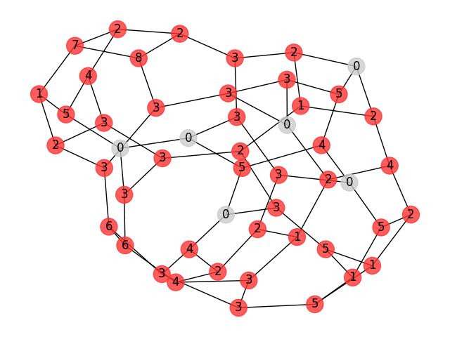
Randomness is understood within a class of graphs, for example regular graphs of given degree, or Erdös–Rényi random graphs. This is related to the following question of Baker.

Question 7.10 (Baker [Bak08]).

Provide a classification of combinatorial graphs without Weierstrass points among their vertices.

References

• [AB15] Omid Amini and Matthew Baker. Linear series on metrized complexes of algebraic curves. Mathematische Annalen, 362(1-2):55–106, 2015.
• [ABBR15] Omid Amini, Matthew Baker, Erwan Brugallé, and Joseph Rabinoff. Lifting harmonic morphisms I: metrized complexes and Berkovich skeleta. Research in the Mathematical Sciences, 2(1):1–67, 2015.
• [ACP15] Dan Abramovich, Lucia Caporaso, and Sam Payne. The tropicalization of the moduli space of curves. Ann. Sci. Éc. Norm. Supér. (4), 48(4):765–809, 2015.
• [AG22] Omid Amini and Lucas Gierczak. Limit linear series: combinatorial theory. arXiv preprint arXiv:2209.15613, 2022.
• [Ami13] Omid Amini. Reduced divisors and embeddings of tropical curves. Transactions of the American Mathematical Society, 365(9):4851–4880, 2013.
• [Ami14] Omid Amini. Equidistribution of Weierstrass points on curves over non-Archimedean fields. arXiv preprint arXiv:1412.0926, 2014.
• [AN22] Omid Amini and Noema Nicolussi. Moduli of hybrid curves II: Tropical and hybrid Laplacians. arXiv preprint arXiv:2203.12785, 2022.
• [AN23] Omid Amini and Noema Nicolussi. Moduli of hybrid curves III: Algebraic geometry of hybrid curves. preprint, 2023.
• [AP03] Scott Ahlgren and Matthew Papanikolas. Higher Weierstrass points on ${X}_{0}(p)$. Transactions of the American Mathematical Society, 355(4):1521–1535, 2003.
• [Arb74] Enrico Arbarello. Weierstrass points and moduli of curves. Compositio Mathematica, 29(3):325–342, 1974.
• [Atk67] A.O.L. Atkin. Weierstrass points at cusps of ${\Gamma}_{0}(n)$. Annals of Mathematics, pages 42–45, 1967.
• [Bak08] Matthew Baker. Specialization of linear systems from curves to graphs. Algebra & Number Theory, 2(6):613–653, 2008.
• [BG95] Edoardo Ballico and Letterio Gatto. On the monodromy of Weierstrass points on Gorenstein curves. Journal of Algebra, 175(2):633–643, 1995.
• [BJ16] Matthew Baker and David Jensen. Degeneration of linear series from the tropical point of view and applications. In Nonarchimedean and Tropical Geometry, pages 365–433. Springer, 2016.
• [BN07] Matthew Baker and Serguei Norine. Riemann–Roch and Abel–Jacobi theory on a finite graph. Advances in Mathematics, 215(2):766–788, 2007.
• [BN16] Matthew Baker and Johannes Nicaise. Weight functions on Berkovich curves. Algebra & Number Theory, 10(10):2053–2079, 2016.
• [BPR13] Matthew Baker, Sam Payne, and Joseph Rabinoff. On the structure of non-Archimedean analytic curves. Tropical and non-Archimedean geometry, 605:93–121, 2013.
• [BS13] Matthew Baker and Farbod Shokrieh. Chip-firing games, potential theory on graphs, and spanning trees. Journal of Combinatorial Theory, Series A, 120(1):164–182, 2013.
• [BT20] Uri Brezner and Michael Temkin. Lifting problem for minimally wild covers of Berkovich curves. Journal of Algebraic Geometry, 29(1):123–166, 2020.
• [CEG08] Caterina Cumino, Eduardo Esteves, and Letterio Gatto. Limits of special Weierstrass points. Int. Math. Res. Pap. IMRP, 2, 2008.
• [CF91] Fernando Cukierman and Lung-Ying Fong. On higher Weierstrass points. Duke Mathematical Journal, 62(1):179–203, 1991.
• [Cuk89] Fernando Cukierman. Families of Weierstrass points. Duke Mathematical Journal, 58(2):317–346, 1989.
• [DC08] Andrea Del Centina. Weierstrass points and their impact in the study of algebraic curves: a historical account from the “Lückensatz” to the 1970s. Annali dell’Universita di Ferrara, 54(1):37–59, 2008.
• [dCS94] Cicero Fernandes de Carvalho and Karl-Otto Stöhr. Higher order differentials and Weierstrass points on Gorenstein curves. Manuscripta Mathematica, 85:361–380, 1994.
• [Dia85] Steven Diaz. Exceptional Weierstrass points and the divisor on moduli space that they define. Mem. Amer. Math. Soc., 56(327), 1985.
• [EH86] David Eisenbud and Joe Harris. Limit linear series: basic theory. Inventiones Mathematicae, 85(2):337–371, 1986.
• [EH87a] David Eisenbud and Joe Harris. Existence, decomposition, and limits of certain Weierstrass points. Inventiones Mathematicae, 87(3):495–515, 1987.
• [EH87b] David Eisenbud and Joe Harris. The Kodaira dimension of the moduli space of curves of genus $\geq 23$. Inventiones Mathematicae, 90(2):359–387, 1987.
• [EM02] Eduardo Esteves and Nivaldo Medeiros. Limit canonical systems on curves with two components. Inventiones Mathematicae, 149(2):267–338, 2002.
• [ES07] Eduardo Esteves and Parham Salehyan. Limit Weierstrass points on nodal reducible curves. Trans. Amer. Math. Soc., 359(10):5035–5056, 2007.
• [Est96] Eduardo Esteves. Wronski algebra systems on families of singular curves. Annales scientifiques de l’École normale supérieure, 29(1):107–134, 1996.
• [Est98] Eduardo Esteves. Linear systems and ramification points on reducible nodal curves. arXiv preprint math/9808069, 1998.
• [Gen21] Quentin Gendron. Sur les nœuds de Weierstraß. Annales Henri Lebesgue, 4:571–589, 2021.
• [GK08] Andreas Gathmann and Michael Kerber. A Riemann–Roch theorem in tropical geometry. Mathematische Zeitschrift, 259(1):217–230, 2008.
• [GL93] Arnaldo García and Robert F. Lax. Weierstrass weight of Gorenstein singularities with one or two branches. Manuscripta Mathematica, 81(1):361–378, 1993.
• [GL95] Arnaldo García and Robert F. Lax. On canonical ideals, intersection numbers, and Weierstrass points on Gorenstein curves. Journal of Algebra, 178(3):807–832, 1995.
• [GL96] Arnaldo García and Robert F. Lax. Rational nodal curves with no smooth Weierstrass points. Proc. Amer. Math. Soc., 124(2):407–413, 1996.
• [HKN13] Jan Hladkỳ, Daniel Král, and Serguei Norine. Rank of divisors on tropical curves. Journal of Combinatorial Theory, Series A, 120(7):1521–1538, 2013.
• [HSS08] Aric A. Hagberg, Daniel A. Schult, and Pieter J. Swart. Exploring network structure, dynamics, and function using NetworkX. In Gaël Varoquaux, Travis Vaught, and Jarrod Millman, editors, Proceedings of the 7th Python in Science Conference, pages 11 – 15, Pasadena, CA USA, 2008.
• [Hun07] J. D. Hunter. Matplotlib: A 2d graphics environment. Computing in Science & Engineering, 9(3):90–95, 2007.
• [Hur92] Adolf Hurwitz. Über algebraische Gebilde mit eindeutigen Transformationen in sich. Mathematische Annalen, 41(3):403–442, 1892.
• [JP22] Dave Jensen and Sam Payne. Tropical linear series and tropical independence. arXiv preprint arXiv:2209.15478, 2022.
• [KRZ16] Eric Katz, Joseph Rabinoff, and David Zureick-Brown. Uniform bounds for the number of rational points on curves of small Mordell–Weil rank. Duke Mathematical Journal, 165(16):3189–3240, 2016.
• [Lak81] Dan Laksov. Weierstrass points on curves. Astérisque, 87(88):221–247, 1981.
• [Lax75] Robert F. Lax. Weierstrass points of the universal curve. Math. Ann., 216:35–42, 1975.
• [Lax87a] Robert F. Lax. On the distribution of Weierstrass points on singular curves. Israel Journal of Mathematics, 57(1):107–115, 1987.
• [Lax87b] Robert F. Lax. Weierstrass points on rational nodal curves. Glasgow Math. J., 29(1):131–140, 1987.
• [Lax87c] Robert F. Lax. Weierstrass weight and degenerations. Proceedings of the American Mathematical Society, pages 8–10, 1987.
• [LF90] John Little and Kathryn A Furio. On the distribution of Weierstrass points on irreducible rational nodal curves. Pacific Journal of Mathematics, 144(1):131–136, 1990.
• [LN64] Joseph Lehner and Morris Newman. Weierstrass points of ${\Gamma}_{0}(n)$. Annals of Mathematics, pages 360–368, 1964.
• [Luo11] Ye Luo. Rank-determining sets of metric graphs. J. Combin. Theory Ser. A, 118(6):1775–1793, 2011.
• [LW90] Robert F. Lax and Carl Widland. Weierstrass points on Gorenstein curves. Pacific Journal of Mathematics, 142(1):197–208, 1990.
• [Nee84] A Neeman. Weierstrass points in characteristic $p$. Inventiones mathematicae, 75(2):359–376, 1984.
• [Ogg78] Andrew P. Ogg. On the Weierstrass points of ${X}_{0}(n)$. Illinois Journal of Mathematics, 22(1):31–35, 1978.
• [Ric18] David Harry Richman. The distribution of Weierstrass points on a tropical curve. arXiv preprint arXiv:1809.07920, 2018.
• [Wei67] Karl Weierstrass. Mathematische Werke, 7 vols (1894–1927) Berlin, reprint by G. Olms, Hildesheim, 1967.