On the Utility of Equal Batch Sizes for Inference in Stochastic Gradient Descent

Abstract

Stochastic gradient descent (SGD) is an estimation tool for large data employed in machine learning and statistics. Due to the Markovian nature of the SGD process, inference is a challenging problem. An underlying asymptotic normality of the averaged SGD (ASGD) estimator allows for the construction of a batch-means estimator of the asymptotic covariance matrix. Instead of the usual increasing batch-size strategy employed in ASGD, we propose a memory efficient equal batch-size strategy and show that under mild conditions, the estimator is consistent. A key feature of the proposed batching technique is that it allows for bias-correction of the variance, at no cost to memory. Since joint inference for high dimensional problems may be undesirable, we present marginal-friendly simultaneous confidence intervals, and show through an example how covariance estimators of ASGD can be employed in improved predictions.

Keywords: Batch-means, Bias correction, Covariance estimation, Confidence regions.

1 Introduction

Robbins and Monro, (1951) marked the inception of a, now popular optimization technique, viz., stochastic gradient descent (SGD). Given the nature of modern data, the increasing popularity of SGD is natural, owing to computational efficiency for large data-sets, and compatibility in online settings (see, e.g., Bottou,, 2010; Bottou et al.,, 2018; Wilson et al.,, 2017).

Let $\Pi$ be a probability distribution on $\mathbb{R}^{r}$; we assume data arises from $\Pi$, denoted by $\zeta\sim\Pi$. In a model fitting paradigm, a function $f:\mathbb{R}^{d}\times\mathbb{R}^{r}\to\mathbb{R}$ typically measures empirical loss for estimating a parameter $\theta$, having observed the data, $\zeta$. Denote the expected loss as $F(\theta)=\mathbb{E}_{\zeta\sim\Pi}\left[f(\theta,\zeta)\right]$. The main parameter of interest is $\theta^{*}\in\mathbb{R}^{d}$ where

$$\theta^{*}=\arg\min_{\theta\in\mathbb{R}^{d}}F(\theta).$$ (1)

With data $\zeta_{i}\overset{\text{iid}}{\sim}\Pi$ for $i=1,\dots,n$, the goal is to estimate $\theta^{*}$. This invariably involves a gradient based technique. Often, $F(\theta)$ is unavailable and a first approximation step is to replace $F(\theta)$ with the empirical loss, $n^{-1}\sum_{i=1}^{n}f(\theta,\zeta_{i})$. When the data are online or when calculation of the complete gradient vector is expensive, a further adjustment is made by replacing the complete gradient with an unbiased estimate. This yields a large class of stochastic gradient algorithms. Denote $\nabla f(\theta,\zeta)$ as the gradient vector of $f(\theta,\zeta)$ with respect to $\theta$, $\eta_{i}>0$ as a learning rate, and $\theta_{0}$ as the starting point of an SGD process. The $i^{\text{th}}$ iterate of SGD is:

$$\theta_{i}=\theta_{i-1}-\eta_{i}\nabla f(\theta_{i-1},\zeta_{i})\,,\qquad\text{ for }i=1,2,\ldots\,\,\,.$$ (2)

Despite the approximations introduced in the optimization, SGD estimates of $\theta$ can have nice statistical properties (Fabian,, 1968; Ruppert,, 1988; Polyak and Juditsky,, 1992), particularly when $\eta_{i}$ is appropriately decreasing and the estimator of $\theta^{*}$ is chosen to be the averaged SGD (ASGD):

$$\hat{\theta}_{n}:=n^{-1}\sum_{i=1}^{n}\theta_{i}\,.$$

Naturally, a point estimate of $\theta^{*}$ alone is not sufficient. The work of Polyak and Juditsky, (1992) has particularly been instrumental in building a framework for statistical inference for $\hat{\theta}_{n}$. Let $A:=\nabla^{2}F(\theta^{*})$ denote the Hessian of $F(\theta)$ evaluated at $\theta=\theta^{*}$ and define $S:=\mathbb{E}_{\Pi}\left([\nabla f(\theta^{*},\zeta)][\nabla f(\theta^{*},\zeta)]^{\top}\right)$. When the derivative and expectation are interchangeable, $\mathbb{E}_{\Pi}\left[\nabla f(\theta^{*},\zeta)\right]=\nabla F(\theta^{*})=0$. Polyak and Juditsky, (1992) showed that if $F$ is strictly convex with a Lipschitz gradient and $\eta_{i}=\eta i^{-\alpha}$ with $\alpha\in(0.5,1)$, then $\hat{\theta}_{n}$ is a consistent estimator of $\theta^{*}$, and under some additional conditions,

$$\sqrt{n}(\hat{\theta}_{n}-\theta^{*})\xrightarrow{\texttt{d}}N(0,\Sigma)\text{ as }n\to\infty,\text{ where }\Sigma=A^{-1}SA^{-1}.$$ (3)

Statistical inference for model parameters is a way forward towards robust implementations of machine learning algorithms. Although there is adequate literature devoted to the convergence behavior of the ASGD estimator and its variants (Zhang,, 2004; Nemirovski et al.,, 2008; Agarwal et al.,, 2012; Zhu and Dong,, 2021), estimators of $\Sigma$ have only recently been developed (Chen et al.,, 2020, 2022; Fang et al.,, 2018; Leung and Chan,, 2022; Zhu et al.,, 2021). Robustness and quality of inference depend critically on the quality of estimation of $\Sigma$.

Chen et al., (2020) proposed two consistent estimators of $\Sigma$: an expensive plug-in estimator that requires repeated computation of the inverse of a Hessian, and a variant of the traditional batch-means estimator of Chen and Seila, (1987) that is cheap to implement. In a batch-means estimator, SGD iterates are broken into batches of possibly differing sizes. A weighted sample covariance of the resulting batch-mean vectors yields a batch-means estimator; the quality of estimation is affected by the choice of batch-sizes. Zhu et al., (2021) proposed a novel increasing batch-size strategy where the size of the batches continually increases until saturation, at which point a new batch is created. We refer to this estimator as the increasing batch-size (IBS) estimator.

Despite the novel batching strategy, finite-sample performance for the IBS estimator is underwhelming; we demonstrate this in a variety of examples. A primary reason for the under-performance is that as iteration size increases, the sample mean vectors of all but the last match cannot improve in quality. We employ equal batch-sizes, that are carefully chosen for both practical utility and theoretical guarantees. Specifically, our proposed batch-sizes are powers of two, where the powers increase as a function of the iteration length. Under mild conditions, our batching strategy yields a consistent estimator and we obtain mean-square-error bounds.

Equal batch-size (EBS) batch-means estimators are common-place in the Markov chain Monte Carlo (MCMC) literature (see, e.g. Geyer,, 1992; Jones et al.,, 2006; Flegal and Jones,, 2010). However, the Markov chains generated by MCMC and SGD are fundamentally different; MCMC typically produces a time-homogeneous, stationary, ergodic chain and SGD produces a time-inhomogeneous and non-stationary chain that converges to a Dirac mass distribution (Dieuleveut et al.,, 2020). Due to these differences, the existing theoretical results of the batch-means estimator of MCMC are not applicable for SGD. However, as we will see, the tools utilized in output analysis for MCMC find use in setting up a workflow for statistical inference in SGD.

The proposed doubling batching structure is developed to allow for finite-sample improvements in the estimation of $\Sigma$. As discussed in Chen et al., (2020); Zhu et al., (2021), due to the Markovian structure of $\{\theta_{i}\}_{i=1}^{n}$, the estimator of $\Sigma$ is often under-biased for any finite $n$; this bias is one of the primary reasons for the underwhelming inferential performance of most estimators of $\Sigma$. Our batching technique allows for a memory-efficient, consistent, and a bias-reduced estimator of $\Sigma$ using the lugsail technique of Vats and Flegal, (2022). Such a bias-reduction technique cannot be applied to IBS estimator of Zhu et al., (2021).

It is worth pausing here to reflect on how do we expect practitioners to use estimators of $\Sigma$? Using the asymptotic normality in (3) and consistent estimators of $\Sigma$, it is possible to implement traditional multivariate hypothesis tests. However, in predictive modeling, this may not be of interest. There is, instead, a need to arrive at marginal-friendly simultaneous confidence intervals for $\theta^{*}$ that allow for easy interpretation. So far, estimators of $\Sigma$ have been employed to make either uncorrected marginal confidence intervals, or uninterpretable ellipsoidal confidence regions. Adapting tools developed in stochastic simulation, we construct marginal confidence intervals with simultaneous coverage that utilize consistent estimators of $\Sigma$.

The rest of the paper is organized as follows. In Section 2 we present our proposed batching strategy. Assumptions and proof of consistency of the resulting batch-means estimator are in Section 3. Section 4, describes the under-estimation problem in estimating $\Sigma$, and discusses bias-correction through a lugsail estimator, which is shown to be consistent as well. Section 5 presents the structure of the marginal-friendly confidence regions. The performance of our proposed estimator is demonstrated through two simulated data problems in Section 6, where the benefits of our proposed estimator are highlighted. In this section, we also present a real data application on a binary classification problem, where we employ the estimator of $\Sigma$ to improve predictions (seen by a reduction in the misclassification error). All proofs are presented in the appendix.

2 Proposed batch-means estimator

2.1 General batch-means estimator

Batch-means estimators and its variants are critical components of output analysis methods in steady-state simulation. A general batch-means estimator can be set up in the following way. For iteration size $n$, the SGD iterates (after some user-chosen warm-up) are divided into $K$ batches with batch-sizes $b_{n,1},\ldots,b_{n,K}$. Let $\tau_{k}=\sum_{j=1}^{k}b_{n,j}$ for $k=1,2,\ldots,K$, denote the ending index for the $k$th batch. Then the batches are:

$$\underbrace{\{\theta_{1},\ldots,\theta_{\tau_{1}}\}}_{1^{\text{st}}\text{ batch}},\underbrace{\{\theta_{\tau_{1}+1},\ldots,\theta_{\tau_{2}}\}}_{2^{\text{nd}}\text{ batch}},\ldots,\underbrace{\{\theta_{\tau_{K-1}+1},\ldots,\theta_{\tau_{K}}\}}_{K^{\text{th}}\text{ batch}}.$$

Let $\bar{\theta}_{k}={b}_{n,k}^{-1}\sum_{i=\tau_{k-1}+1}^{\tau_{k}}\theta_{i}$ denote the mean vector of the $k^{\text{th}}$ batch. A general batch-means estimator is

$$\hat{\Sigma}_{\text{gen}}=\dfrac{1}{K}\sum_{k=1}^{K}b_{n,k}\left(\bar{\theta}_{k}-\hat{\theta}_{n}\right)\left(\bar{\theta}_{k}-\hat{\theta}_{n}\right)^{\top}\,.$$ (4)

Batch-means estimators of limiting covariances are commonplace in steady-state simulation (Chen and Seila,, 1987; Glynn and Whitt,, 1991; Chien et al.,, 1997) and MCMC (Chakraborty et al.,, 2022; Liu and Flegal,, 2018; Vats et al.,, 2019). Their performance is critically dependent on the batching structure; this choice is process dependent and much work has gone into their study for ergodic and stationary Markov chains (Damerdji,, 1995; Liu et al.,, 2022).

In the context of SGD, batch-means estimators were recently adopted in the sequence of works by Chen et al., (2020); Zhu and Dong, (2021); Zhu et al., (2021). For $\eta_{i}=i^{-\alpha}$, $\alpha\in(1/2,1)$, the batch-size chosen by Zhu et al., (2021) is

$$b_{n,k}\propto k^{\frac{1+\alpha}{1-\alpha}}\,.$$ (5)

The above choice is motivated by the following argument: if $b_{n,k}$ is reasonably large, the batch-mean vector is approximately normally distributed. Using Chen et al., (2020, Equation 15), for large $j$ and $k$ ($>j$), the strength of correlation between $\theta_{j}$ and $\theta_{k}$ is

$$\prod_{i=j}^{k-1}\|I_{d}-\eta_{i+1}A\|\leq\exp\left(-\lambda_{\min}(A)\sum_{i=j}^{k-1}\eta_{i+1}\right),$$ (6)

where $\lambda_{\min}(A)$ is the smallest eigenvalue of $A$. Consequently, if $\sum_{i=j}^{k-1}\eta_{i+1}$ is sufficiently large, the $j^{\text{th}}$ and $k^{\text{th}}$ iterates are approximately uncorrelated. Therefore, for large $b_{n,k}$’s, batch-mean vectors are approximately independent and normally distributed. The batch-size in (5), is such that $\sum_{i=j}^{k-1}\eta_{i+1}$ is sufficiently large. This reasoning ignores the dangers of choosing large batch-sizes. For any given iteration length, larger batch-sizes implies smaller number of batches leading to high variance and/or singular estimators of $\Sigma$. Consequently, the quality of inference is challenged and multivariate inference becomes difficult.

2.2 Proposed batching strategy

Under an equal batch-size strategy, $b_{n,k}=b_{n}$ for all $k$; the number of batches is $a_{n}:=K=\lfloor n/b_{n}\rfloor$. With this choice, the estimator in (4) simplifies to

$$\hat{\Sigma}_{b_{n}}=a_{n}^{-1}\sum_{k=1}^{a_{n}}b_{n}(\bar{\theta}_{k}-\hat{\theta}_{n})(\bar{\theta}_{k}-\hat{\theta}_{n})^{\top}= ~{}\cfrac{b_{n}}{a_{n}}\displaystyle\sum\limits_{k=1}^{a_{n}}\bar{\theta}_{k}\bar{\theta}_{k}^{\top}-b_{n}\hat{\theta}_{n}\hat{\theta}_{n}^{\top}.$$ (7)

Choosing $b_{n}\propto\lfloor n^{\beta}\rfloor$ for some $\beta\in(0,1)$ seems natural, and is often considered in stochastic simulation. However, in order to implement the bias-reduction procedure along with reduced memory costs, the above is impractical. Instead, for some $c>0$ and current iterate $n$, consider batch-sizes of the following form:

$$b_{n}^{*}=\min\{2^{\gamma}:cn^{\beta}\leq 2^{\gamma}\text{ for }\gamma\in\mathbb{N}\}\,.$$ (8)

That is, $b_{n}^{*}$ is the smallest power of 2 that is bounded below by $cn^{\beta}$. Naturally, $cn^{\beta}\leq b_{n}^{*}\leq 2cn^{\beta}$, and $a_{n}^{*}:=n/b_{n}^{*}$ for any given $n$ is bounded like $n^{1-\beta}/(2c)\leq a_{n}^{*}\leq n^{1-\beta}/c$. A similar batch-size strategy was hinted at in Gong and Flegal, (2016). A pictorial demonstration of the batching strategy is in Figure 1, for the settings discussed in Section 6. Naturally, as $n\to\infty$, both $b_{n}^{*}$ and $a_{n}^{*}$ tend to $\infty$. Since $b_{n}^{*}$ and $a_{n}^{*}$ oscillates within two polynomial functions of $n$, our asymptotic results use $b_{n}=cn^{\beta}$; the practical implementations utilize $b_{n}^{*}$. The proposed batching structure reduces storage costs to only $a_{n}$ batch-mean vectors at any given stage; $a_{n}=O(n^{1-\beta})$ dramatically smaller than $n$. Further, for the iterate of $n$ when batch-size changes, new batches are just made by averaging over adjacent batch-mean vectors; at these moments the number of batches gets halved.

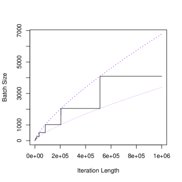
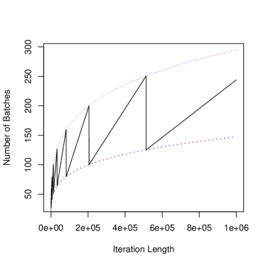
Figure 1: Pictorial demonstration of the proposed batching structure, as a function of $n$; settings are chosen in accordance with the simulations in Section 6. Purple dotted lines are polynomial rates that bound the batch-size (left) and number of batches (right).

3 Main results

Consistency of $\hat{\Sigma}_{b_{n}}$ along with the asymptotic normality result of Polyak and Juditsky, (1992) in (3), allows for large-sample inferential procedures, similar to traditional maximum likelihood estimation. For this task, we make assumptions that ensure both the asymptotic normality in (3) and consistency of the covariance estimator.

3.1 Notations and assumptions

For a vector $x\in\mathbb{R}^{d}$, let $\|x\|$ denote the Euclidean norm and for a matrix $A$, let $\|A\|$ denote its matrix norm. All norms are equivalent in a finite-dimensional Euclidean space, so in the following discussion, we can replace the matrix norm with any other norm.

• (On $F$). Let the objective function $F$ be such that the following hold:

  1. $F(\theta)$ is continuously differentiable and strongly convex with parameter $M>0$. That is, for any $\theta_{1}$ and $\theta_{2}$,

     $$F(\theta_{2})\geq F(\theta_{1})+\nabla F(\theta_{1})^{\top}(\theta_{2}-\theta_{1})+\frac{M}{2}\|\theta_{2}-\theta_{1}\|^{2}.$$ (9)

  2. The gradient vector $\nabla F(\theta)$ is Lipschitz continuous with constant $L_{F}$, that is, for any $\theta_{1}$ and $\theta_{2}$,

     $$\|\nabla F(\theta_{1})-\nabla F(\theta_{2})\|\leq L_{F}\|\theta_{1}-\theta_{2}\|\,.$$ (10)

  3. The Hessian of $F$ at $\theta^{*}$, $A=\nabla^{2}F(\theta^{*})$ exists, and there exists $L_{1}$ such that

     $$\|A(\theta-\theta^{*})-\nabla F(\theta)\|\leq L_{1}\|\theta-\theta^{*}\|^{2}.$$

Assumption (A1) is important for the convergence and asymptotic normality of $\hat{\theta}_{n}$ (see Polyak and Juditsky,, 1992; Moulines and Bach,, 2011; Rakhlin et al.,, 2012). The strong convexity of $F$ implies that $\lambda_{\min}(A)\geq M$, which is an important condition for parameter estimation (see Chen et al., 2020; Zhu et al., 2021; Zhu and Dong, 2021). Further, this will be a key ingredient for proving consistency of the batch-means estimator of $\Sigma$.

• (On $f$ and $\zeta_{i}$). Let $D_{i}=\theta_{i}-\theta^{*}$, $\xi_{i}=\nabla F(\theta_{i-1})-\nabla f(\theta_{i-1},\zeta_{i})$, and $\mathbb{E}_{i}(\cdot)$ denotes the conditional expectation $\mathbb{E}(\cdot|\zeta_{i},\zeta_{i-1},\ldots,\zeta_{1})$, then the following hold:

  1. The function $f(\theta,\zeta)$ is continuously differentiable in $\theta$ for any $\zeta$ and $\|\nabla f(\theta,\zeta)\|$ is uniformly integrable for any $\theta$ (so that $\mathbb{E}_{i-1}(\xi_{i})=0$).

  2. The conditional covariance of $\xi_{i}$ has an expansion around $\theta=\theta^{*}$. That is, $\mathbb{E}_{i-1}[\xi_{i}\xi_{i}^{\top}]=S+\mathcal{H}(D_{i-1})$, and there exist constants $\sigma_{1}$ and $\sigma_{2}$ such that for any $D\in\mathbb{R}^{d}$,

     $$\|\mathcal{H}(D)\|\leq\sigma_{1}\|D\|+\sigma_{2}\|D\|^{2}\text{ and }|\operatorname{tr}(\mathcal{H}(D))|\leq\sigma_{1}\|D\|+\sigma_{2}\|D\|^{2}.$$

  3. There exists constants $\sigma_{3}$ and $\sigma_{4}$ such that the fourth conditional moment of $\xi_{i}$ is bounded, i.e., $\mathbb{E}_{i-1}\|\xi_{i}\|^{4}\leq\sigma_{3}+\sigma_{4}\|D_{i-1}\|^{4}$.

Assumption (A2)(i) allows $\mathbb{E}_{\zeta\sim\Pi}\left[\nabla f(\theta,\zeta)\right]=\nabla F(\theta)$, which implies that the sequence $\{\xi_{i}\}$ is a martingale difference process. These assumptions are standard (see Chen et al.,, 2020; Zhu et al.,, 2021) and ensure the regularity of the noisy gradients.

Our next set of conditions are on the learning rate and the choice of equal batch-size. Our results are general for any choice of batch-size satisfying the condition below.

• (On $\eta_{i}$, $b_{n}$) The following hold:

  1. The learning rate is $\eta_{i}=\eta i^{-\alpha}$ with $\alpha\in(0.5,1),i=1,2,3,\ldots~{}$.

  2. $b_{n}$ is size of the batch such that $b_{n}n^{-\alpha}\to\infty$ and $b_{n}n^{-1}\to 0$ as $n\to\infty$.

In Assumption (A3)(i), the learning rate is that of Polyak and Juditsky, (1992), ensuring asymptotic normality. Assumption(A3)(ii) is the only additional condition added to this statistical inference setup that is specific to our choice of batch-size. Our chosen $b_{n}=cn^{\beta}$ satisfies this condition for $\beta\in(\alpha,1)$ (and thus $b_{n}^{*}$ satisfies this condition as well). As a consequence of Assumption (A3)(i),

$$\sum_{i=\tau_{k-1}+1}^{\tau_{k}}\eta_{i}=\sum_{i=\tau_{k-1}+1}^{\tau_{k}}\eta i^{-\alpha}>\eta b_{n}{\tau_{k}}^{-\alpha}>\eta b_{n}n^{-\alpha}=:N.$$ (11)

Using Assumption (A3)(ii), $N\to\infty$ as $n\to\infty$. This guarantees that the batch-size is larger than the persistent correlation in the SGD iterates. That is, using (6), this ensures fast decay of correlation between batches, which is a critical step in proving consistency of the batch-means estimator.

In the following discussion, for sequences of positive numbers $p_{n}$ and $q_{n}$, denote

• $p_{n}\gtrsim q_{n}$ if for some $c>0,cp_{n}\geq q_{n}$ for all $n$ large enough,

• $p_{n}\lesssim q_{n}$ if $q_{n}\gtrsim p_{n}$, and

• $p_{n}\asymp q_{n}$ if $p_{n}\gtrsim q_{n}$ and $p_{n}\lesssim q_{n}$.

For simplicity, we define the following constant, which may depend on $d$

$$C_{d}:=\max\left\{L_{F},L_{1},\sigma_{1}^{2/3},\sqrt{\sigma_{2}},\sqrt{\sigma_{3}},\sigma_{4}^{1/4},\operatorname{tr}(S)\right\}.$$

3.2 Consistency of the estimator

We now present our main result of consistency of the batch-means estimator with fixed batch-size.

Theorem 1.

Under the assumptions (A1), (A2) and (A3), for sufficiently large $n$

$$~{}\mathbb{E}\big{\|}\hat{\Sigma}_{b_{n}}-\Sigma\big{\|}\lesssim~{}C_{d}^{2}n^{-\alpha/2+(\beta-1)/4}+C_{d}^{3}n^{-\alpha}+C_{d}a_{n}^{-1/2}+C_{d}b_{n}^{\alpha-1}+C_{d}b_{n}^{-1/2}n^{\alpha/2}+C_{d}a_{n}^{-1}+C_{d}^{4}{n}^{-2\alpha}{b_{n}}.$$

Proof.

Proof is available in Appendix C. ∎

Under Assumption (A3), the bound in Theorem 1 goes to zero, yielding consistency of $\hat{\Sigma}_{b_{n}}$. Chen et al., (2020, Theorem 4.3) and Zhu et al., (2021, Theorem 3.1) provide similar bounds for different IBS batch-means estimators, with Zhu et al., (2021) being an improvement over Chen et al., (2020). One key reason for explicitly writing a bound instead of merely mentioning convergence to zero, is that the bound allows for a reasonable choice for $b_{n}$. Substituting batch-sizes of the form $b_{n}=cn^{\beta}$, in Theorem 1,

$$~{}\mathbb{E}\big{\|}\hat{\Sigma}_{b_{n}}-\Sigma\big{\|}\lesssim~{}n^{-\alpha/2+(\beta-1)/4}+n^{(\beta-1)/2}+n^{-\beta(1-\alpha)}+n^{(\alpha-\beta)/2}+n^{\beta-1}+{n}^{\beta-2\alpha}.$$ (12)

Obtaining a closed-form expression of an optimal $\beta$ from the right side of the above equation is challenging. A numerical solution is possible, but not interpretable. Instead, we note that by Assumption (A3), $(\beta-1)/2>\beta-2\alpha$ and $-\alpha/2+(\beta-1)/4<(\beta-1)/2$, so among the first, second, fifth, and sixth terms, the second term is dominating. Further, $-\beta(1-\alpha)<(\alpha-\beta)/2$, so among the third and fourth terms, the fourth term is dominating. Considering then, only the dominating terms, we have

$$\mathbb{E}\big{\|}\hat{\Sigma}_{b_{n}}-\Sigma\big{\|}\lesssim n^{(\beta-1)/2}+n^{(\alpha-\beta)/2}.$$

With this approximation, the optimal choice of $\beta$ is $\beta^{*}={(1+\alpha)}/{2}\,$.

Remark 1.

The bounds we obtain are meaningful only for large $n$. For small $n$, it is challenging to obtain a meaningful expression of the optimal value of $\beta$. Numerically, we observed that for sample size of the order $O(10^{3})$ and $\alpha=0.51$, the optimal value of $\beta$ is near $0.66$. However, as $n$ increase, the optimal value of $\beta$ approaches $(1+\alpha)/2$. This agrees with the above mentioned bound.

Remark 2.

Consistency of $\hat{\Sigma}_{b_{n}}$ immediately allows the construction of Wald-like confidence regions (see Section 5). To obtain a consistent estimator of $\Sigma$, the number of batches, $a_{n}$, must increase with $n$. Naturally, the batch-size also must be large to mimic the limiting Polyak and Juditsky, (1992) behavior. This yields a challenging trade-off. Our particular batch-size construction allows finite-sample adjustments for small batch sizes using the lugsail trick (see Section 4). If the goal is only inference, and not the quantification of variance, Zhu and Dong, (2021) proposed a method of consistent estimation based on a fixed number of batches.

4 Bias-reduced estimation

Naturally, the mean-square bound in Theorem 1 is contributed from both the bias and variance of the batch-means estimator. As also argued by Simonoff, (1993), controlling the bias of variance estimators is more important than controlling its variance, particularly when the bias is in the negative direction. For this reason Vats and Flegal, (2022) proposed a lugsail batch-means estimator for stochastic simulation that can dramatically reduce bias in variance estimation. Our particular choice of equal batch-size allows an easy and effective implementation of the lugsail technique. Obtaining an exact expression of the bias of the batch-means estimator for a general SGD framework is an open problem. However, the following mean estimation model provides a motivation.

Example 1.

Consider for $i=1,2,\dots,n$, a mean estimation model $y_{i}=\theta^{*}+\epsilon_{i}$, where $\theta^{*}\in\mathbb{R}$ and $\epsilon_{i}$ are independent mean-zero random error terms. For the squared error loss function $f(\theta,\zeta)=(y-\theta)^{2}/2$ for estimating $\theta^{*}$, the $i^{\text{th}}$ SGD iterate is

$$\theta_{i}=\theta_{i-1}+\eta_{i}(y_{i}-\theta_{i-1})\,,$$

with $\eta_{i}=\eta i^{-{\alpha}}$. In Appendix D, we show that the bias of $\hat{\Sigma}_{b_{n}}$ for this model is:

$$\operatorname{Bias}(\hat{\Sigma}_{b_{n}})\approx\frac{-2C_{1}}{n}\sum_{1\leq j<k\leq a_{n}}\sum_{p=\tau_{j-1}+1}^{\tau_{j}}\sum_{q=\tau_{k-1}+1}^{\tau_{k}}q^{-\alpha}(1-q^{-\alpha})^{q-p}\,,$$

where $C_{1}$ is a positive constant. The estimator of Zhu et al., (2021) exhibits a similar negative bias expression. For large $n$, the bias may be insignificant, however, as Figure 2 exhibits, even in this simple model, the finite-sample bias in the estimator of $\Sigma$ remains significant.

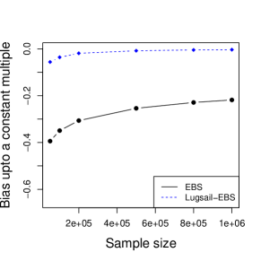
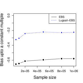
Figure 2: Mean estimation model: Bias of the EBS and Lugsail-EBS estimator for $\alpha=0.51$ (left) and $\alpha=0.75$ (right) against sample size.

More than the magnitude of bias, its direction is a larger concern. Variance estimation of any statistical estimator allows us to assess the uncertainty in the problem. Under-estimation of this variance leads to a false sense of security and inadequate tests (see Simonoff,, 1993, for e.g.). Obtaining bias-free estimators for such long-run variances is a critical and challenging problem in operations research, stochastic simulation, econometrics, and MCMC. A wide range of solutions have been attempted (Kiefer and Vogelsang,, 2002, 2005; Liu and Flegal,, 2018; Politis and Romano,, 1995) to reduce the bias of variance estimators.

By allowing lag-windows in spectral variance estimators to partially increase, Vats and Flegal, (2022) develop a family of variance estimators, called lugsail estimators, that are essentially obtained by a carefully chosen linear combination of variance estimators. In the context of steady-state simulation and MCMC, this leads to a flexible and consistent class of bias-corrected variance estimators. Specifically, the lugsail batch-means estimator is

$$\hat{\Sigma}_{L,b_{n}}:=2\hat{\Sigma}_{2b_{n}}-\hat{\Sigma}_{b_{n}}.$$ (13)

Our batching strategy, $b_{n}^{*}$, allows an easy implementation of the lugsail bias-correction strategy since a batch-means estimator of batch-size $2b_{n}^{*}$ can be obtained by combining adjacent batch-means vectors. Thus, the proposed bias-correction does not increase memory costs. We also note that since the lugsail lag-windows rely on equal batch-sizes, such lugsail corrections are not directly possible for the IBS estimator. We call the estimator in (13) the lugsail-EBS estimator.

For the mean estimation model in Example 1, Figure 2 presents the bias expression of both EBS and the lugsail-EBS estimators. Although the bias in the estimator depends on the correlation in the process (through $\alpha$ in this case), in both cases, the lugsail-EBS estimator presents significant bias reduction. As we will see in Section 6, this correction proves to be critical for finite-sample inference.

The following theorem establishes the consistency of the lugsail-EBS estimator, under the same conditions as required in Theorem 1.

Theorem 2.

Under Assumptions (A1), (A2) and (A3), for sufficiently large $n$,

$$\mathbb{E}\big{\|}\hat{\Sigma}_{L,b_{n}}-\Sigma\big{\|}\lesssim ~{}5C_{d}^{2}n^{-\alpha/2+(\beta-1)/4}+5C_{d}^{3}n^{-\alpha}+6C_{d}a_{n}^{-1/2}+5C_{d}b_{n}^{\alpha-1}+4C_{d}b_{n}^{-1/2}n^{\alpha/2}$$

$$~{}+9C_{d}a_{n}^{-1}+9C_{d}^{4}{n}^{-2\alpha}{b_{n}}.$$

Proof.

Proof is provided in Appendix D.2. ∎

Theorem 2 guarantees the consistency of $\hat{\Sigma}_{L,b_{n}}$. The bound in Theorem 2 is larger than that in Theorem 1; this is purely a consequence of the proof technique.

5 Marginal and simultaneous inference

For problems where SGD is relevant, it is natural to ask what purpose will an estimator of $\Sigma$ serve? Zhu et al., (2021) use the diagonals of $\Sigma$ to construct uncorrected marginal confidence intervals for each of the $d$ parameters of interest. The problem of multiple-testing is omnipresent in this case, and corrections like Bonferroni can be crude. Moreover, the potentially complex dependence in $\Sigma$, via both $S$ and $A$ is completely ignored. On the other hand, a $d$-dimensional confidence ellipsoid is not tenable for marginal-friendly inference. For this reason, marginal-friendly simultaneous inference is essential in practice.

For joint inference for $\theta^{*}$, (3) provides a $100(1-p)\%$ confidence ellipsoid

$$E_{p}=\left\{\theta\in\mathbb{R}^{d}:(\hat{\theta}_{n}-\theta)^{\top}\hat{\Sigma}^{-1}_{n}(\hat{\theta}_{n}-\theta)\leq\chi^{2}_{d,1-p}\right\},$$ (14)

where $\chi^{2}_{d,s}$ denotes the $s$th quantile of a chi-squared distribution with $d$ degrees of freedom. Marginal interpretation of such an ellipsoid confidence region is difficult. Instead, one may study marginal confidence intervals. Let $\hat{\Sigma}_{n}$ be any consistent estimator of $\Sigma$. Let $\hat{\theta}_{n}=(\hat{\theta}_{n1},\ldots,\hat{\theta}_{nd})^{\top}$, $\theta^{*}=(\theta^{*}_{1},\ldots,\theta^{*}_{d})^{\top}$ and $\hat{\Sigma}_{n}=(\hat{\sigma}_{ij})_{i,j=1,\dots,p}$. Using (3), for $0<p<1$, an asymptotic $100(1-p)\%$ marginal confidence interval of $\theta^{*}_{i}$ is:

$$\hat{\theta}_{ni}\pm z_{1-p/2}\sqrt{\hat{\sigma}_{ii}/n}\,,$$ (15)

where $z_{s}$ denotes the $s$th quantile of $N(0,1)$. Fang et al., (2018), Chen et al., (2020), Zhu et al., (2021), and Zhu and Dong, (2021) discuss both uncorrected marginal confidence intervals and the ellipsoid joint confidence region. As discussed, both are inconducive for valid and interpretable joint inference. For the general Monte Carlo problem, Robertson et al., (2021) suggest a remedy by using an appropriate hyper-rectangular confidence region, which we now describe. Using the $d$ uncorrected intervals in (15), an at-most $100(1-p)\%$ hyper-rectangular confidence region is

$$C_{lb}(z_{p/2})=\prod_{i=1}^{d}[\hat{\theta}_{ni}-z_{1-p/2}\sqrt{\hat{\sigma}_{ii}/n},\,\hat{\theta}_{ni}+z_{1-p/2}\sqrt{\hat{\sigma}_{ii}/n}]\,.$$

Using a Bonferroni approach, an at least $100(1-p)\%$ hyper-rectangular confidence region is

$$C_{ub}(z_{p/2d})=\prod_{i=1}^{d}[\hat{\theta}_{ni}-z_{1-p/2d}\sqrt{\hat{\sigma}_{ii}/n},\,\hat{\theta}_{ni}+z_{1-p/2d}\sqrt{\hat{\sigma}_{ii}/n}]\,.$$

Clearly, $C_{lb}(z_{p/2})\subseteq C_{ub}(z_{p/2d}).$ Robertson et al., (2021) suggested a quasi Monte-Carlo approach to find a $z^{*}$ with $z_{1-p/2}<z^{*}<z_{1-p/2d}$ to yield the hyper-rectangular confidence region

$$C(z^{*})=\prod_{i=1}^{d}[\hat{\theta}_{ni}-z^{*}\sqrt{\hat{\sigma}_{ii}/n},\,\hat{\theta}_{ni}+z^{*}\sqrt{\hat{\sigma}_{ii}/n}]\,,$$ (16)

such that $C_{lb}(z_{p/2})\subseteq C(z^{*})\subseteq C_{ub}(z_{p/2d})$ and $\mathbb{P}(\theta^{*}\in C(z^{*}))\approx 1-p$, under the assumption that $\hat{\theta}_{n}\approx N_{p}(\theta_{*},\hat{\Sigma}_{n})$. An illustration is given by Figure 3. The computation of (16) is essentially a quick one-dimensional optimization problem solved by bisection search over the interval $(z_{1-p/2},z_{1-p/2d})$; see Robertson et al., (2021) for details. In Section 6, we present coverage properties of both the ellipsoidal region $E_{p}$ and the cuboidal region $C(z^{*})$.

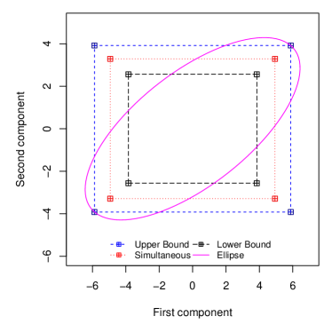
Figure 3: Plot of $C_{lb}(z_{p/2})$ (black dashed) and $C_{ub}(z_{p/2d})$ (blue dashed) from a $90\%$ confidence region for a bivariate normal distribution with component variances 9 and 4. The red dashed line gives the corresponding $C({z^{*}})$.

6 Numerical implementations

6.1 Setup

We implement our proposed EBS and lugsail-EBS estimators for two simulated models and a real data implementation. We systematically keep the following settings for our EBS estimator: $c=0.1$ so that the number of batches stays reasonably large ensuring that the estimator is positive-definite; $\beta=(1+\alpha)/2$ as a reasonable value obtained from the mean-square bounds; $\alpha=0.51$ to allow for reasonable exploration. For comparison we implement the IBS estimator of Zhu et al., (2021) with their suggested settings. However, in the event that the IBS estimator is singular, we increase their number of batches to also allow positive-definiteness of the IBS estimator.

When the true covariance matrix $\Sigma$ is available, we employ it as an oracle, and use it to calculate the relative Frobenius norm of an estimator $\hat{\Sigma}$: $\|\hat{\Sigma}-\Sigma\|_{F}/\|\Sigma\|_{F}$. Further, we employ $\Sigma$ in calculating the coverage probability of the confidence regions discussed in Section 5. To this coverage, we compare the coverage probabilities obtained using various estimators of $\Sigma$. Another important feature of confidence regions is its volume, particularly for the cuboidal regions created in (16). Thus, for each estimator, we also report

$$\left(\dfrac{\text{Volume}(C(z^{*}))}{\text{Volume}(E_{p})}\right)^{1/p}\,$$

for a which a high value indicates an undesired increase in the volume of the confidence region. Reproducible codes are available at https://github.com/Abhinek-Shukla/SGD-workflow.

6.2 Linear regression

We simulate data according to the linear regression model, for $i=1,2,\dots,n$, $y_{i}=x_{i}^{T}\beta^{*}+\epsilon_{i}$ where for some $d\times d$ positive-definite matrix $A$, $x_{i}\overset{\text{iid}}{\sim}N(0,A)$ and $\epsilon_{i}\overset{\text{iid}}{\sim}N(0,1)$, independent of $x_{i}$. We fix $\beta^{*}\in\mathbb{R}^{d}$ to be the $d$-vector of equidistant points on the grid $(0,1)$. Here $\zeta_{i}=(x_{i},y_{i})$. In order to implement ordinary least squares estimation of $\beta$, the loss function is

$$f(\beta,\zeta_{i})=\cfrac{\big{(}y_{i}-x_{i}^{\top}\beta\big{)}^{2}}{2}.$$

Since the errors are iid, the true $\Sigma$ is $A^{-1}$. We consider the three forms of $A$ used in Chen et al., (2020): (i) identity ($A=I_{d}$), (ii) Toeplitz, where element $A_{i,j}=\rho^{|i-j|}$, and (iii) Equicorrelation, where element $A_{i,j}=\rho$ for $i\neq j$ and $1$ otherwise. Throughout, we set $\rho=0.5$. We present results of all three settings of $A$ for $d=5$ (here $\eta=0.5$) and for brevity, only present the identity result for $d=20$ (here $\eta=1$).

Data of size $5\times 10^{6}$ was simulated with the first 1000 SGD iterates being discarded as burn-in. We start the SGD process from $\bm{0}$ and study the statistical performance of various estimators of $\Sigma$ sequentially as a function of the data. Since the above is done for 1000 replications, for each $A$ and $d$, we present four key comparative plots: (i) The estimated relative Frobenius norm as a function of the sample size, (ii) The estimated ellipsoidal coverage probabilities, (iii) the estimated coverage probabilities of the cuboidal confidence regions, and (iv) the ratio of the volumes of the cuboidal regions to the ellipsoidal regions.

Figure 4 presents the results for $d=5$. Due to the nature of the batching technique, the performance is not monotonic as a function of the sample size for EBS; this is expected. However, for each of the three settings, the lugsail-EBS estimator outperforms in all measures with the EBS being competitive with the IBS estimator, when not better. One metric where the IBS estimator suffers drastically, are the marginal confidence regions. As evident from Figure 4, the coverage for the IBS estimator improves drastically when going from the elliptical regions to the cuboidal regions. The bottom row of the plots indicate that this is entirely due to the drastic increase in the volume of region. The cuboidal regions made by IBS are significantly larger that their ellipsoidal regions. This is likely due to an exaggerated correlation structure captured by the IBS. Both the EBS estimators, and particularly the lugsail-EBS do not suffer from this. These problems are further exaggerated for $d=20$ as evidenced in Figure 5. The performance of both EBS and lugsail-EBS remains essentially the same. We highlight that even when the relative Frobenius norm is large for the EBS estimators, the simultaneous marginal coverage probabilities are reasonable, with only little cost to the volume.

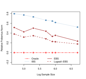
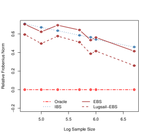
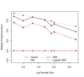
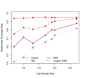
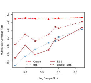
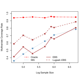
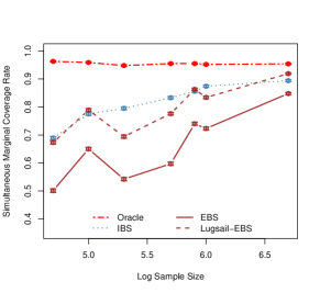
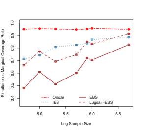
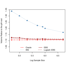
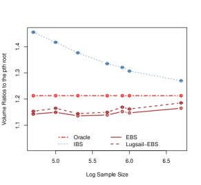
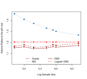
Figure 4: Linear regression $d=5$: Line plots equipped with error bars from 1000 replications. Left plots for $A$ being identity, middle plots for $A$ being Toeplitz, and right plots for $A$ being equicorrelation matrix.

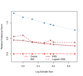
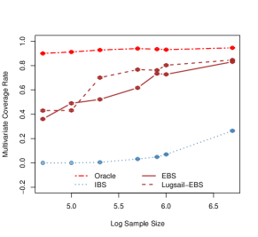
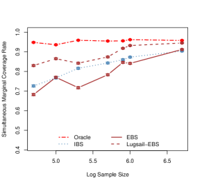
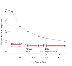
Figure 5: Linear regression $d=20$ for identity $A$: Line plots equipped with error bars from 1000 replications

To understand why the EBS performs significantly better than the IBS estimators, we take a closer look at the batching strategy. The general idea in batch-means estimators is that each batch-mean vector emulates the sample mean ASGD estimator; thus the empirical sample covariance of these batch-means is a reasonable estimator of $\Sigma$. For such a heuristic to hold, the batch-mean vector for each batch must be approximately normally distributed; $\sqrt{b_{n,k}}\bar{\theta}_{k}\approx N_{d}(\theta^{*},I_{d})$. For $d=5$ with $A$ being identity, if we accumulate all the components of all batch-mean vectors they should be normally distributed, and thus we may compare them with true Gaussian quantiles. In Figure 6, we present a zoomed-in QQ plot of this for two different data sizes. Figure 6 reveals significant deviation from normality for the IBS estimator, particularly for small sample situations. The EBS estimator, on the other hand, follows the theoretical Gaussian quantiles fairly well.

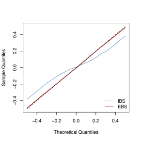
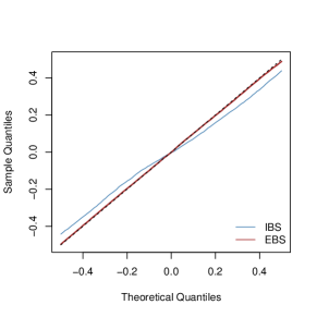
Figure 6: Linear regression for $d=5$: QQ plot of all components of the batch-means vectors in the IBS and the EBS estimators, with black lines indicating theoretical quantiles. Left panel is corresponding to $n=50000$ and right panel is corresponding to $n=10^{6}$.

6.3 LAD regression

Assume a similar linear regression model, with non-Gaussian errors: $y_{i}=x_{i}^{T}\beta^{*}+\epsilon_{i}$ where $x_{i}\overset{\text{iid}}{\sim}N(0,A)$ and $\epsilon_{i}\overset{\text{iid}}{\sim}\text{DE}(0,1)$, here $\text{DE}(\mu,\lambda)$ denotes the double exponential distribution with median parameter $\mu$ and scale parameter $\lambda$. Instead of ordinary least squares, we consider the least absolute deviation (LAD) loss function, $f(\beta,\zeta_{i})={\big{|}y_{i}-x_{i}^{\top}\beta\big{|}}$. Fang et al., (2018) consider this simulation setup as well and discuss that the true $\Sigma$ is $A^{-1}$.

We repeat the simulation setup of the previous section with $d=20$ for the three different choices of $A$. Figure 7 presents the results. The performance of the EBS estimators, particularly lugsail-EBS is significantly superior to that of the IBS estimator. Here again, although the simultaneous coverage of the cuboidal regions is far improved for the IBS estimator, this is purely a consequence of over-inflated volume of the region.

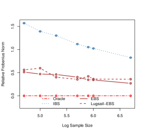
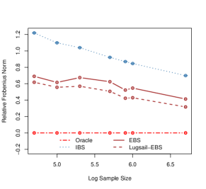
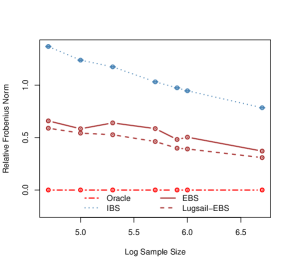
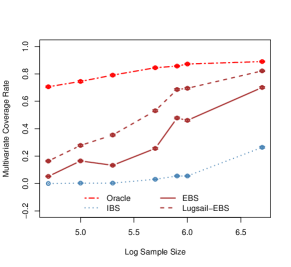
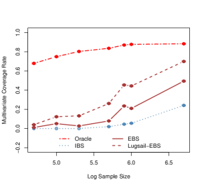
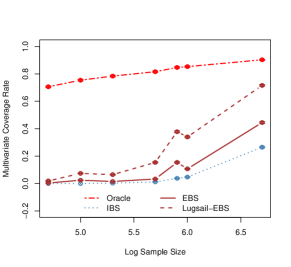
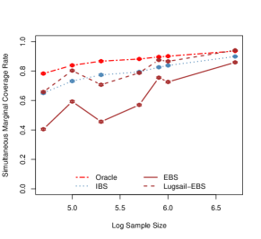
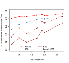
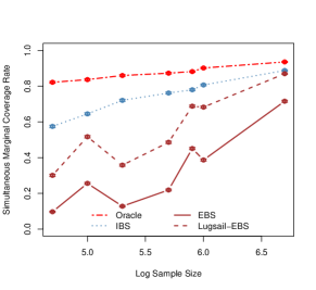
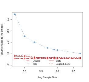
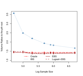
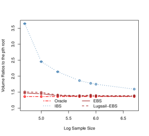
Figure 7: LAD regression for $d=20$: Line plots equipped with error bars from 1000 replications. Left plots for $A$ being identity, middle plots for $A$ being Toeplitz, and right plots for $A$ being equicorrelation matrix.

6.4 Santander customer transaction data

Consider the Santander customer transaction dataset, which contains 200 features on $2\times 10^{5}$ bank transactions. The response is a binary variable indicating whether the transaction is of a certain type. We split the data evenly into training and testing, and then employ logistic regression to predict transaction type. For $i=1,2,\dots,$, assume

$$y_{i}\sim\text{Bernoulli}\left(p_{i}:=\dfrac{1}{1+e^{-x_{i}^{\top}\beta^{*}}}\right),$$

where $x_{i}$ are assumed to be iid. For estimation, the loss function is the negative log-likelihood as a consequence of the Bernoulli model assumption. We implement ASGD with $\eta=.05$ starting the process at the maximum-likelihood estimate of the first 10000 observations. The next 5000 data points were employed in a burn-in, yielding an SGD sequence of length 85000. Since the true $\beta^{*}$ and $\Sigma$ are unknown, comparison of confidence regions is unreasonable here. We can obtain marginal simultaneous confidence intervals, however due to the nature of the data, classical hypothesis testing may not be of interest. Instead, we utilize the estimator of $\Sigma$ for prediction.

In most applications where SGD is employed, estimates of $\beta^{*}$ are used in predictions, without any focus on accounting for the variability is its estimation. Denote the ASGD estimator of $\beta^{*}$ with $\hat{\beta}_{n}$, and for any data point $j$, the fitted/predicted probability of success is estimated with

$$\hat{p}_{j}:=\dfrac{1}{1+e^{-x_{j}^{\top}\hat{\beta}_{n}}}\,.$$

A thresholding is then typically used to obtain a binary prediction of this $j$th observation, based on $\hat{p}_{j}$. That is, for some user-chosen threshold $q$, $\hat{y}_{j}=\mathbb{I}(\hat{p}_{j}>q)$. When employing a test dataset, misclassification rates can then be obtained for model building and comparisons. Due to (3) and the delta method, as $n\to\infty$,

$$\sqrt{n}(\hat{p}_{j}-p_{j})\overset{d}{\to}N\left(0,(p_{j}(1-p_{j}))^{2}x_{j}^{\top}\Sigma x_{j}\right)\,.$$

Since our proposed EBS estimator of $\Sigma$ is consistent, we can obtain a confidence interval for each $\hat{p}_{j}\pm z_{.975}\,\,\text{se}_{j}$, where the standard error is calculated using the plug-in estimators of $\Sigma$ and $p_{j}$. In order to account for the estimation variability in $\hat{p}_{j}$, we employ an alternative estimator of $y_{j}$: $\tilde{y}_{j}=\mathbb{I}(\hat{p}_{j}-z_{.975}\,\,\text{se}_{j}>q)$. That is, our logistic classifier, classifies the observation as a success if the lower-bound on the confidence interval for $\hat{p}_{j}$ is larger than the cutoff, $q$; different observations will have different se_j. Figure 8 demonstrates the misclassification rate for our test data for various values of $q$, using both the above methods. Clearly, the blue curve which employs the EBS estimator to obtain se_j yields a lower misclassification rate. Due to consistency of the estimator, se_j is expected to converge to 0 as $n\to\infty$, and thus, for a large enough training data, we would expect the blue and the black curves to merge into one.

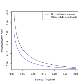
Figure 8: Misclassification rate on the testing set for various values of the cutoff.

7 Discussion

Our proposed EBS batching-strategy can be extended to averaging over $k$-neighbouring batches for any fixed positive integer $k$, and all the theoretical results discussed will hold true. However, large values of $k$ will reduce the number of batches, thereby reducing the efficiency of the covariance estimator. Leung and Chan, (2022) discuss variants the IBS estimator and find that their performances are quite similar. A study similar Leung and Chan, (2022) for the EBS estimator would make a useful follow-up of our work. Building a statistical inference framework for SGD is an active area of research in recent times. This includes the recent works of Fang et al., (2018); Xie et al., (2023) who use bootstrap techniques to estimate the limiting covariance structure. Fang et al., (2018) heuristically argued to use the (perturbed) bootstrap ASGD outputs to estimate the covariance matrix of $\hat{\theta}_{n}$. The theoretical properties of the estimator are not known and computational demands of the estimator is considerable. Zhu and Dong, (2021) present a method of consistent inference for SGD without using a consistent estimator of $\Sigma$. It remains unclear if methods of marginal inference and delta method arguments can be used in their framework. Li et al., (2023); Liu et al., (2023) estimate the limiting covariance under situations when the iid assumption on the data is violated. Our marginal-friendly confidence interval construction, and utilization of $\Sigma$ in improving predictions are directly applicable to this literature.

There are numerous other variants of the SGD (see, e.g., Konečný et al.,, 2016; Toulis and Airoldi,, 2017; Loizou and Richtárik,, 2020; Yuan and Ma,, 2020), and the fundamental framework remains essentially the same for other variants of SGD, as long as the results of Polyak and Juditsky, (1992) applies to them. For example, Toulis and Airoldi, (2017) obtained asymptotic normality of averaged implicit SGD, and the framework we present here can be seamlessly transferred to that setup.

Finally, we employ the estimator of $\Sigma$ in two tasks: (i) the construction of marginal-friendly simultaneous confidence intervals that favor interpretability over ellipsoidal regions, and (ii) construct confidence intervals around predictions for new observations. The logistic regression example we present in Section 6.4 demonstrates this feature. A similar argument can yield prediction intervals for regression as well, one which accounts for the multivariate estimation error in the SGD estimates.

8 Acknowledgements

The authors are thankful to Prof. Jing Dong for useful conversations. Dootika Vats is supported by SERB (SPG/2021/001322) and Google Asia Pacific Pte Ltd.

Appendix A Preliminary results

Lemma 1.

Under the assumption (A3), we have

1. $\tau_{k-1}=(k-1)b_{n}\asymp kb_{n}$, $\tau_{k}=kb_{n}\asymp(k-1)b_{n}$ and $\tau_{k-1}\asymp\tau_{k}\asymp kn^{\beta}$.

2. $\sum_{i=\tau_{k-1}+1}^{\tau_{k}}\eta_{i}>\eta b_{n}{\tau_{k}}^{-\alpha}>\eta b_{n}n^{-\alpha}=:N$.

3. For any fixed $\gamma>0$ and $\gamma\neq 1$, $T^{-1}\sum_{k=1}^{T}k^{-\gamma}\lesssim T^{-1}\int_{1}^{T+1}x^{-\gamma}dx\lesssim T^{-\gamma}$.

4. For any fixed $\gamma>0$, $\sum_{k=1}^{T}k^{\gamma}\leq\int_{1}^{T}(x+1)^{\gamma}~{}dx\lesssim T^{1+\gamma}$.

Proof.

Proofs of 1) and 2) are obvious. For the proof of 3), observe that

$$T^{-1}\sum_{k=1}^{T}k^{-\gamma}\leq T^{-1}\left[1+\int_{1}^{T+1}x^{-\gamma}dx\right]\lesssim T^{-1}\int_{1}^{T+1}x^{-\gamma}dx\lesssim T^{-\gamma}.$$

Next, for the proof of 4), we have

$$\sum_{k=1}^{T}k^{\gamma}\leq\int_{1}^{T}(x+1)^{\gamma}~{}dx\leq\frac{1}{1+\gamma}(T+1)^{\gamma+1}\lesssim T^{1+\gamma}.$$

∎

The following three results from Chen et al., (2020) will be used in our proofs.

Result 1 (Chen et al., (2020), Lemma D.2).

For each positive integer $j$, let $Y_{j}^{k}$ be a sequence of matrices with $Y_{j}^{j}=I$ and for $k\geq j$, $Y_{j}^{k}=(I-\eta_{k}A)Y_{j}^{k-1}=\prod_{i=j}^{k}(I-\eta_{i}A)$, where $A$ is a PSD matrix with eigen values bounded below by $\lambda_{A}>0$. Then, under the assumption (A3), we have

• For $i\in\{j,\ldots,k\}$, the following holds

  $$\|Y_{j}^{k}\|\leq\exp\left(-\lambda_{A}\sum_{i=j+1}^{k}\eta_{i}\right)\leq\exp\left(-\lambda_{A}(k-j)\eta_{k}\right).$$

• Let $S_{j}^{k}=\sum_{i=j+1}^{k}Y_{j}^{i}$ and $Z_{j}^{k}=\eta_{j}S_{j}^{k}-A^{-1}$, then

  $$\|S_{j}^{k}\|\lesssim k^{\alpha},~{}\|Z_{j}^{k}\|\lesssim k^{\alpha}j^{-1}+exp\left(-\lambda_{A}\sum_{i=j}^{k}\eta_{i}\right).$$

• When $1\leq j<k\leq\tau_{a_{n}}$, for sufficiently large $N$, there exists a constant $c$ such that

  $$\|S_{j}^{k}\|\lesssim j^{\alpha},~{}\|Z_{j}^{k}\|\lesssim j^{\alpha-1}+\exp\left(-c\lambda_{A}(k-j)\eta_{j}\right),~{}\|\eta_{j}S_{j}^{k}\|\lesssim 1,$$

  as long as $a_{n}\leq N^{q}$ for certain positive integer $q$.

Result 2 (Chen et al., (2020), Lemma D.3).

Let $S$ and $\Sigma$ are two $d\times d$ matrices, and $S$ is positive definite, then $\operatorname{tr}(S\Sigma)\leq\operatorname{tr}(S)\|\Sigma\|$.

Result 3 (Chen et al., (2020), Lemma 3.2).

Under the assumptions (A1) and (A2), there exists $n_{0}$ such that the iterate error $D_{n}$ satisfy the following:

• For $n>m\geq n_{0}$,

  • $\mathbb{E}_{m}\|D_{n}\|\lesssim\exp\left(\frac{-1}{4}M\sum_{i=m}^{n}\eta_{i}\right)\|D_{m}\|+\sqrt{C_{d}}m^{-\alpha/2}$,

  • $\mathbb{E}_{m}\|D_{n}\|^{2}\lesssim\exp\left(\frac{-1}{4}M\sum_{i=m}^{n}\eta_{i}\right)\|D_{m}\|^{2}+{C_{d}}m^{-\alpha}$, and

  • $\mathbb{E}_{m}\|D_{n}\|^{4}\lesssim\exp\left(\frac{-1}{4}M\sum_{i=m}^{n}\eta_{i}\right)\|D_{m}\|^{4}+{C_{d}}^{2}m^{-2\alpha}$.

• • $\mathbb{E}\|D_{n}\|\lesssim n^{-\alpha/2}(\sqrt{C_{d}}+\|D_{n_{0}}\|)$,

  • $\mathbb{E}\|D_{n}\|^{2}\lesssim n^{-\alpha}({C_{d}}+\|D_{n_{0}}\|^{2})$, and

  • $\mathbb{E}\|D_{n}\|^{4}\lesssim n^{-2\alpha}({C_{d}}^{2}+\|D_{n_{0}}\|^{4})$.

Appendix B Auxiliary sequence

An approximation of the SGD iterate is $D_{i}\simeq(I_{d}-\eta_{i}A)D_{i-1}+\eta_{i}\xi_{i}$. We replace $\simeq$ by $=$ to obtain an approximated iterate sequence,

$$U_{i}=(I_{d}-\eta_{i}A)U_{i-1}+\eta_{i}\xi_{i},~{}U_{0}=D_{0}.$$ (17)

The sequence $\{U_{i}\}$ is known as the auxiliary sequence. The following result for the sequence $\{U_{i}\}$ from Chen et al., (2020) is helpful.

Result 4 (Chen et al., (2020), Lemma B.3).

For the sequence $U_{i}$, under the assumptions (A1) and (A2), we have

$$\mathbb{E}\|U_{n}\|^{2}\lesssim n^{-\alpha}(C_{d}+\|U_{0}\|^{2}+\|D_{0}\|^{2}).$$

Lemma 2.

Under the assumptions (A1), (A2) and (A3), we have

$$\hat{S}:=\frac{1}{a_{n}}\sum_{k=1}^{a_{m}}\frac{1}{b_{n}}\left(\sum_{i=\tau_{k-1}+1}^{\tau_{k}}\xi_{i}\right)\left(\sum_{i=\tau_{k-1}+1}^{\tau_{k}}\xi_{i}\right)^{\top}$$

is a consistent estimator of $S$, precisely,

$$\mathbb{E}\|\hat{S}-S\|^{2}\lesssim C_{d}^{4}n^{-\alpha+(\beta-1)/2}+C_{d}^{6}n^{-2\alpha}+C_{d}^{2}a_{n}^{-1}.$$

Proof.

Let $\widetilde{\xi}_{i}=-\Delta f(\theta^{*},\zeta_{i})$, $\widehat{\xi}_{i}=\xi_{i}-\widetilde{\xi}_{i}$ and

$$\widetilde{S}=\frac{1}{a_{n}}\sum_{k=1}^{a_{n}}\frac{1}{b_{n}}\left(\sum_{i=\tau_{k-1}+1}^{\tau_{k}}\widetilde{\xi}_{i}\right)\left(\sum_{i=\tau_{k-1}+1}^{\tau_{k}}\widetilde{\xi}_{i}\right)^{\top}.$$

Then, $\xi_{i}=\hat{\xi}_{i}+\widetilde{\xi}_{i}$ where $\{\widetilde{\xi}_{i}\}$ is a sequence of iid RVs and $\{\hat{\xi}_{i}\}$ is a martingale difference sequence. Note that

$$\mathbb{E}\|\hat{S}-S\|^{2}\lesssim\mathbb{E}\|\widetilde{S}-S\|^{2}+\mathbb{E}\|\hat{S}-\widetilde{S}\|^{2},$$ (18)

and

$$\mathbb{E}\|\widetilde{S}-S\|^{2}\leq\mathbb{E}\operatorname{tr}(\widetilde{S}-S)^{2}=\operatorname{tr}\mathbb{E}(\widetilde{S}-S)^{2}.$$ (19)

Further

$$\mathbb{E}(\widetilde{S})=\frac{1}{a_{n}}\sum_{k=1}^{a_{n}}\frac{1}{b_{n}}\sum_{i=\tau_{k-1}+1}^{\tau_{k}}\mathbb{E}(\widetilde{\xi}_{i}\widetilde{\xi}_{i}\,^{\top})=S,$$

therefore $\mathbb{E}(\widetilde{S}-S)^{2}=\mathbb{E}(\widetilde{S}^{2})-S^{2}$. Next

$$\mathbb{E}\widetilde{S}^{2}=a_{n}^{-2}\sum_{j=1}^{a_{n}}\sum_{k=1}^{a_{n}}b_{n}^{-2}\sum_{i_{1},i_{2}=\tau_{j-1}+1}^{\tau_{j}}\sum_{i_{3},i_{4}=\tau_{k-1}+1}^{\tau_{k}}\mathbb{E}(\widetilde{\xi}_{i_{1}}\widetilde{\xi}_{i_{2}}^{\top}\widetilde{\xi}_{i_{3}}\widetilde{\xi}_{i_{4}}^{\top}).$$

Since $\{\widetilde{\xi}_{i}\}$ is an iid sequence of RVs, on the RHS of the above expression, the terms are zero unless $i_{1}=i_{2}$, $i_{3}=i_{4}$ or $i_{1}=i_{3}$, $i_{2}=i_{4}$ or $i_{1}=i_{4}$, $i_{2}=i_{3}$. Also, the latter two only happen when all the indices are in the same batch, thus

$$\mathbb{E}\widetilde{S}^{2}= ~{}a_{n}^{-2}\sum_{j=1}^{a_{n}}\sum_{k=1}^{a_{n}}b_{n}^{-2}\sum_{i_{1}=\tau_{j-1}+1}^{\tau_{j}}\sum_{i_{3}=\tau_{k-1}+1}^{\tau_{k}}\mathbb{E}(\widetilde{\xi}_{i_{1}}\widetilde{\xi}_{i_{1}}^{\top}\widetilde{\xi}_{i_{3}}\widetilde{\xi}_{i_{3}}^{\top})$$

$$+a_{n}^{-2}\sum_{j=1}^{a_{n}}b_{n}^{-2}\sum_{i_{1},i_{3}=\tau_{j-1}+1,i_{1}\neq i_{3}}^{\tau_{j}}[\mathbb{E}(\widetilde{\xi}_{i_{1}}\widetilde{\xi}_{i_{3}}^{\top}\widetilde{\xi}_{i_{1}}\widetilde{\xi}_{i_{3}}^{\top})+\mathbb{E}(\widetilde{\xi}_{i_{1}}\widetilde{\xi}_{i_{3}}^{\top}\widetilde{\xi}_{i_{3}}\widetilde{\xi}_{i_{1}}^{\top})].$$

Using $\mathbb{E}(\widetilde{\xi}_{i_{1}}\widetilde{\xi}_{i_{1}}^{\top}\widetilde{\xi}_{i_{3}}\widetilde{\xi}_{i_{3}}^{\top})=S^{2}$ if $i_{1}\neq i_{3}$, we get

$$\operatorname{tr}(\mathbb{E}\widetilde{S}^{2}-S^{2})=a_{n}^{-2}\sum_{j=1}^{a_{n}}b_{n}^{-2}\sum_{i_{1},i_{3}=\tau_{j-1}+1,i_{1}\neq i_{3}}^{\tau_{j}}[\mathbb{E}(\widetilde{\xi}_{i_{1}}\widetilde{\xi}_{i_{3}}^{\top}\widetilde{\xi}_{i_{1}}\widetilde{\xi}_{i_{3}}^{\top})+\mathbb{E}(\widetilde{\xi}_{i_{1}}\widetilde{\xi}_{i_{3}}^{\top}\widetilde{\xi}_{i_{3}}\widetilde{\xi}_{i_{1}}^{\top})].$$

Next using $\mathbb{E}(\widetilde{\xi}_{i_{1}}\widetilde{\xi}_{i_{1}}^{\top}\widetilde{\xi}_{i_{3}}\widetilde{\xi}_{i_{3}}^{\top})\lesssim C_{d}^{2}+C_{d}^{6}i_{1}^{-2\alpha}$ if $i_{1}=i_{3}$, we obtain

$$\operatorname{tr}(\mathbb{E}\widetilde{S}^{2}-S^{2})= ~{}a_{n}^{-2}\sum_{j=1}^{a_{n}}b_{n}^{-2}\left(\sum_{i_{1}=\tau_{j-1}+1}^{\tau_{j}}\mathbb{E}\|\widetilde{\xi}_{i_{1}}\|^{4}+\sum_{i_{1},i_{3}=\tau_{j-1}+1,i_{1}\neq i_{3}}^{\tau_{j}}(\mathbb{E}(\widetilde{\xi}_{i_{1}}^{\top}\widetilde{\xi}_{i_{3}})^{2}+\mathbb{E}(\|\widetilde{\xi}_{i_{1}}\|^{2}\|\widetilde{\xi}_{i_{3}}\|^{2}))\right)$$

$$\lesssim ~{}a_{n}^{-2}\sum_{j=1}^{a_{n}}\left(b_{n}^{-1}(C_{d}^{2}+C_{d}^{6}\tau_{j}^{-2\alpha})+(\operatorname{tr}(S))^{2}\right).$$

Consequently using Lemma 1

$$\operatorname{tr}(\mathbb{E}\widetilde{S}^{2}-S^{2})\lesssim ~{}C_{d}^{2}n^{-1}+C_{d}^{6}a_{n}^{-(1+2\alpha)}+C_{d}^{2}a_{n}^{-1}.$$ (20)

Next, we denote

$$\widecheck{S}=\frac{1}{a_{n}}\sum_{k=1}^{a_{n}}\frac{1}{b_{n}}\left(\sum_{i=\tau_{k-1}+1}^{\tau_{k}}\hat{\xi}_{i}\right)\left(\sum_{i=\tau_{k-1}+1}^{\tau_{k}}\hat{\xi}_{i}\right)^{\top}.$$

We notice that

$$\mathbb{E}\|\hat{S}-\widetilde{S}\|^{2}= ~{}\mathbb{E}\left\|{a_{n}}^{-1}\sum_{k=1}^{a_{n}}{b_{n}}^{-1}\left(\left(\sum_{i=\tau_{k-1}+1}^{\tau_{k}}\widetilde{\xi}_{i}\right)\left(\sum_{i=\tau_{k-1}+1}^{\tau_{k}}\hat{\xi}_{i}\right)^{\top}+\left(\sum_{i=\tau_{k-1}+1}^{\tau_{k}}\hat{\xi}_{i}\right)\left(\sum_{i=\tau_{k-1}+1}^{\tau_{k}}\widetilde{\xi}_{i}\right)^{\top}\right)+2\widecheck{S}\right\|^{2}$$

$$\lesssim ~{}\mathbb{E}\left\|{a_{n}}^{-1}\sum_{k=1}^{a_{m}}{b_{n}}^{-1}\left(\sum_{i=\tau_{k-1}+1}^{\tau_{k}}\widetilde{\xi}_{i}\right)\left(\sum_{i=\tau_{k-1}+1}^{\tau_{k}}\hat{\xi}_{i}\right)^{\top}\right\|^{2}+\mathbb{E}\|\widecheck{S}\|^{2}$$

$$\lesssim ~{}\sqrt{\mathbb{E}(\operatorname{tr}(\widecheck{S}^{2}))}\sqrt{\mathbb{E}(\operatorname{tr}(\widetilde{S}^{2}))}+\mathbb{E}(\operatorname{tr}(\widecheck{S}^{2})).$$ (21)

Now we need to find a bound for $\mathbb{E}(\operatorname{tr}(\widecheck{S}^{2}))$. Let $\widebar{\xi}_{k}=b_{n}^{-1}\sum_{i=\tau_{k-1}+1}^{\tau_{k}}\hat{\xi}_{i}$. Then using Cauchy-Schwartz inequality, we have

$$\mathbb{E}(\operatorname{tr}(\widecheck{S}^{2}))= ~{}{a_{n}}^{-2}\sum_{k=1}^{a_{n}}\sum_{l=1}^{a_{n}}{b_{n}}^{2}\,\mathbb{E}(\operatorname{tr}(\widebar{\xi}_{k}\widebar{\xi}_{k}^{\top}\widebar{\xi}_{l}\widebar{\xi}_{l}^{\top}))\lesssim{a_{n}}^{-2}\sum_{k=1}^{a_{n}}\sum_{l=1}^{a_{n}}{b_{n}}^{2}\,\sqrt{\mathbb{E}\|\widebar{\xi}_{k}\|^{4}}\sqrt{\mathbb{E}\|\widebar{\xi}_{l}\|^{4}}$$

$$\lesssim ~{}{a_{n}}^{-2}\sum_{k=1}^{a_{n}}\sum_{l=1}^{a_{n}}{b_{n}}^{-2}\,\sum_{i=\tau_{k-1}+1}^{\tau_{k}}\sqrt{\mathbb{E}\|\hat{\xi}_{i}\|^{4}}\sum_{j=\tau_{l-1}+1}^{\tau_{l}}\sqrt{\mathbb{E}\|\hat{\xi}_{j}\|^{4}},\text{using Theorem 2.1 in \cite[cite]{\@@bibref{Authors Phrase1YearPhrase2}{rio2009moment}{\@@citephrase{(}}{\@@citephrase{)}}}}.$$

Using Result 3, we have $\mathbb{E}\|\hat{\xi}_{j}\|_{2}^{4}\lesssim C_{d}^{6}i^{-2\alpha}$. Consequently using Lemma 1 we get

$$\mathbb{E}(\operatorname{tr}(\widecheck{S}^{2}))\lesssim C_{d}^{6}(n^{-1}\sum_{i=1}^{n}i^{-\alpha})(n^{-1}\sum_{j=1}^{n}j^{-\alpha})\lesssim C_{d}^{6}n^{-2\alpha}.$$

Further substituting in (21) we have

$$\mathbb{E}\|\hat{S}-\widetilde{S}\|^{2}\lesssim C_{d}^{4}n^{-\alpha+(\beta-1)/2}+C_{d}^{6}n^{-2\alpha}.$$ (22)

Combining (18), (19), (20), (21) and (22), completes the proof. ∎

Define overall mean and batch means of $U_{i}$ as follows:

$$\bar{U}_{n}=\frac{1}{\tau_{a_{n}}}\sum_{i=1}^{\tau_{a_{n}}}U_{i}\text{ and }\bar{U}_{k}=\frac{1}{b_{n}}\sum_{i=\tau_{k-1}+1}^{\tau_{k}}U_{i}\text{ for }k=1,2,\ldots,a_{n}.$$

Lemma 3.

Under the assumptions (A1), (A2) and (A3), we have

$$\mathbb{E}\bigg{\|}a_{n}^{-1}\sum_{k=1}^{a_{n}}b_{n}\bar{U}_{k}\bar{U}_{k}^{\top}-A^{-1}SA^{-1}\bigg{\|}\lesssim ~{}C_{d}^{2}n^{-\alpha/2+(\beta-1)/4}+C_{d}^{3}n^{-\alpha}+C_{d}a_{n}^{-1/2}+C_{d}b_{n}^{\alpha-1}+C_{d}b_{n}^{-1/2}n^{\alpha/2}.$$

Proof.

The recursion of $U_{j}$ can be written as

$$U_{i}= ~{}Y_{i-1}^{i}U_{i-1}+Y_{i}^{i}\eta_{i}\xi_{i}=~{}Y_{i-2}^{i}U_{i-2}+Y_{i-1}^{i}\eta_{i-1}\xi_{i-1}+Y_{i}^{i}\eta_{i}\xi_{i}$$

$$= ~{}Y_{j}^{i}U_{j}+\sum_{l=j+1}^{i}Y_{l}^{i}\eta_{l}\xi_{l}.$$

Therefore, the $k^{th}$ batch mean $\bar{U}_{k}$ can be written as

$$\bar{U}_{k}= ~{}b_{n}^{-1}\left(\sum_{i=\tau_{k-1}+1}^{\tau_{k}}Y_{\tau_{k-1}}^{i}U_{\tau_{k-1}}+\sum_{i=\tau_{k-1}+1}^{\tau_{k}}\sum_{l=\tau_{k-1}+1}^{i}Y_{l}^{i}\eta_{l}\xi_{l}\right)$$

$$= ~{}b_{n}^{-1}\left[\sum_{i=\tau_{k-1}+1}^{\tau_{k}}Y_{\tau_{k-1}}^{i}U_{\tau_{k-1}}+\sum_{l=\tau_{k-1}+1}^{\tau_{k}}\left(\sum_{i=l}^{\tau_{k}}Y_{l}^{i}\right)\eta_{l}\xi_{l}\right]$$

$$= ~{}b_{n}^{-1}\left[\sum_{i=\tau_{k-1}+1}^{\tau_{k}}Y_{\tau_{k-1}}^{i}U_{\tau_{k-1}}+\sum_{l=\tau_{k-1}+1}^{\tau_{k}}\left(S_{l}^{\tau_{k}}+I\right)\eta_{l}\xi_{l}\right]$$

$$= ~{}b_{n}^{-1}S_{\tau_{k-1}}^{\tau_{k}}U_{\tau_{k-1}}+b_{n}^{-1}A^{-1}\sum_{l=\tau_{k-1}+1}^{\tau_{k}}\xi_{l}+b_{n}^{-1}\sum_{l=\tau_{k-1}+1}^{\tau_{k}}\xi_{l}Z_{l}^{\tau_{k}}+b_{n}^{-1}\sum_{l=\tau_{k-1}+1}^{\tau_{k}}\eta_{l}\xi_{l}.$$

Let us denote

$$A_{k}:=-A^{-1}\sum_{l=\tau_{k-1}+1}^{\tau_{k}}\xi_{l}\text{ and }B_{k}:=S_{\tau_{k-1}}^{\tau_{k}}U_{\tau_{k-1}}+\sum_{l=\tau_{k-1}+1}^{\tau_{k}}\xi_{l}Z_{l}^{\tau_{k}}+\sum_{l=\tau_{k-1}+1}^{\tau_{k}}\eta_{l}\xi_{l}.$$

Then,

$$a_{n}^{-1}\sum_{k=1}^{a_{n}}b_{n}\bar{U}_{k}\bar{U}_{k}^{\top}=a_{n}^{-1}\sum_{k=1}^{a_{n}}b_{n}^{-1}A_{k}A_{k}^{\top}+a_{n}^{-1}\sum_{k=1}^{a_{n}}b_{n}^{-1}[A_{k}B_{k}^{\top}+B_{k}A_{k}^{\top}+B_{k}B_{k}^{\top}].$$ (23)

We have from Lemma 2,

$$\mathbb{E}\bigg{\|}a_{n}^{-1}\sum_{k=1}^{a_{n}}b_{n}^{-1}A_{k}A_{k}^{\top}-A^{-1}SA^{-1}\bigg{\|}^{2}= ~{}\mathbb{E}\bigg{\|}A^{-1}(\hat{S}-S)A^{-1}\bigg{\|}^{2}$$

$$\lesssim ~{}C_{d}^{4}n^{-\alpha+(\beta-1)/2}+C_{d}^{6}n^{-2\alpha}+C_{d}^{2}a_{n}^{-1}.$$ (24)

Using Cauchy Schwartz inequality, we have

$$\mathbb{E}\bigg{\|}a_{n}^{-1}\sum_{k=1}^{a_{n}}b_{n}^{-1}A_{k}A_{k}^{\top}-A^{-1}SA^{-1}\bigg{\|}\lesssim C_{d}^{2}n^{-\alpha/2+(\beta-1)/4}+C_{d}^{3}n^{-\alpha}+C_{d}a_{n}^{-1/2}.$$

Using $\|B_{k}\|^{2}=\|B_{k}B_{k}^{\top}\|\leq\operatorname{tr}(B_{k}B_{k}^{\top})$ and $\xi_{i}$ is a martingale, we have

$$~{}\mathbb{E}B_{k}B_{k}^{\top}$$

$$= ~{}\mathbb{E}\Bigg{[}S_{\tau_{k-1}}^{\tau_{k}}U_{\tau_{k-1}}+\sum_{l=\tau_{k-1}+1}^{\tau_{k}}\xi_{l}Z_{l}^{\tau_{k}}+\sum_{l=\tau_{k-1}+1}^{\tau_{k}}\eta_{l}\xi_{l}\bigg{]}\Bigg{[}S_{\tau_{k-1}}^{\tau_{k}}U_{\tau_{k-1}}+\sum_{l=\tau_{k-1}+1}^{\tau_{k}}\xi_{l}Z_{l}^{\tau_{k}}+\sum_{l=\tau_{k-1}+1}^{\tau_{k}}\eta_{l}\xi_{l}\bigg{]}^{\top}$$

$$= ~{}S_{\tau_{k-1}}^{\tau_{k}}\mathbb{E}\left[U_{\tau_{k-1}}U_{\tau_{k-1}}^{\top}\right](S_{\tau_{k-1}}^{\tau_{k}})^{\top}+\sum_{l=\tau_{k-1}+1}^{\tau_{k}}(Z_{l}^{\tau_{k}}+\eta_{l}I)\mathbb{E}(\xi_{l}\xi_{l}^{\top})(Z_{l}^{\tau_{k}}+\eta_{l}I)^{\top}.$$

$$\Rightarrow ~{}\operatorname{tr}(\mathbb{E}B_{k}B_{k}^{\top})\leq\|S_{\tau_{k-1}}^{\tau_{k}}\|^{2}\mathbb{E}\|U_{\tau_{k-1}}\|^{2}+\sum_{l=\tau_{k-1}+1}^{\tau_{k}}\|Z_{l}^{\tau_{k}}+\eta_{l}I\|^{2}\mathbb{E}\|\xi_{l}\|^{2}.$$

Now, using Result 1, we have

$$\|Z_{l}^{\tau_{k}}+\eta_{l}I\|\leq\|Z_{l}^{\tau_{k}}\|+\eta l^{-\alpha}\lesssim l^{\alpha-1}+\exp\left(-c\lambda_{A}(\tau_{k}-l)\eta_{l}\right)+l^{-\alpha}.$$

Using $l^{-\alpha}<l^{\alpha-1}$ for $\alpha\in(0.5,1)$ and Cauchy-Schwartz inequality, we get

$$\|Z_{l}^{\tau_{k}}+\eta_{l}I\|^{2}\lesssim l^{2\alpha-2}+\exp\left(-2c\lambda_{A}(\tau_{k}-l)\eta_{l}\right).$$

Next, using the bound of $\|U_{n}\|^{2}$ in Result 4, and $\mathbb{E}\|\xi_{l}\|^{2}\lesssim C_{d}$, we obtain

$$\frac{1}{C_{d}}\operatorname{tr}\left(\mathbb{E}B_{k}B_{k}^{\top}\right)\lesssim ~{}(\tau_{k-1}+1)^{\alpha}+\sum_{l=\tau_{k-1}+1}^{\tau_{k}}\|Z_{l}^{\tau_{k}}+\eta_{l}I\|^{2}$$

$$\lesssim ~{}(\tau_{k-1}+1)^{\alpha}+b_{n}(\tau_{k-1}+1)^{2\alpha-2}+\sum_{l=\tau_{k-1}+1}^{\tau_{k}}\exp\left(-2c\lambda_{A}(\tau_{k}-l)\eta_{\tau_{k-1}+1}\right)$$

$$\lesssim ~{}(\tau_{k-1}+1)^{\alpha}+b_{n}(\tau_{k-1}+1)^{2\alpha-2}+\sum_{l=0}^{\infty}\exp\left(-2c\lambda_{A}l\eta_{\tau_{k-1}+1}\right)$$

$$\lesssim ~{}(\tau_{k-1}+1)^{\alpha}+b_{n}(\tau_{k-1}+1)^{2\alpha-2}+\left(2c\lambda_{A}\eta_{\tau_{k-1}+1}\right)^{-1}.$$

Using

$$b_{n}(\tau_{k-1}+1)^{2\alpha-2}+\left(2c\lambda_{A}\eta_{\tau_{k-1}+1}\right)^{-1}= ~{}b_{n}(k-1)^{2\alpha-2}b_{n}^{2\alpha-2}+(k-1)^{-\alpha}b_{n}^{-\alpha}\frac{1}{2c\lambda_{A}}$$

$$\lesssim ~{}(k-1)^{2\alpha-2}b_{n}^{2\alpha-1}+(k-1)^{-\alpha}b_{n}^{-\alpha}\lesssim b_{n}^{2\alpha-1},$$

and Lemma 1 (claim 4), we have

$$a_{n}^{-1}\sum_{k=1}^{a_{n}}b_{n}^{-1}\mathbb{E}\|B_{k}\|^{2}\lesssim ~{}C_{d}a_{n}^{-1}\sum_{k=1}^{a_{n}}b_{n}^{-1}(b_{n}^{2\alpha-1}+(\tau_{k-1}+1)^{\alpha})$$

$$\leq ~{}C_{d}b_{n}^{2\alpha-2}+C_{d}a_{n}^{-1}\sum_{k=1}^{a_{n}}b_{n}^{-1}(\tau_{k-1}+1)^{\alpha}$$

$$\leq ~{}C_{d}b_{n}^{2\alpha-2}+C_{d}b_{n}^{-1}n^{\alpha}.$$ (25)

On the other hand, using martingale property of $\xi_{i}$, we have

$$b_{n}^{-1}\mathbb{E}\|A_{k}\|^{2}= ~{}b_{n}^{-1}\operatorname{tr}\left(\mathbb{E}A_{k}A_{k}^{\top}\right)=b_{n}^{-1}\operatorname{tr}\left(A^{-1}\mathbb{E}\left(\sum_{i=\tau_{k-1}+1}^{\tau_{k}}\xi_{i}\right)\left(\sum_{i=\tau_{k-1}+1}^{\tau_{k}}\xi_{i}\right)^{\top}A^{-1}\right)$$

$$\leq ~{}b_{n}^{-1}\|A^{-1}\|^{2}\left[b_{n}\operatorname{tr}(S)+2\sum_{i=\tau_{k-1}+1}^{\tau_{k}}\mathbb{E}(\sigma_{1}\|D_{i}\|+\sigma_{2}\|D_{i}\|^{2})\right]\lesssim C_{d}.$$ (26)

So, using (B), B and Cauchy Schwartz inequality, we get

$$b_{n}^{-1}\mathbb{E}\|A_{k}\|\|B_{k}\|\lesssim\sqrt{b_{n}^{-1}\mathbb{E}\|A_{k}\|^{2}}\sqrt{b_{n}^{-1}\mathbb{E}\|B_{k}\|^{2}}\lesssim C_{d}b_{n}^{\alpha-1}+C_{d}b_{n}^{-1/2}n^{\alpha/2}.$$ (27)

Thus, using (23), (B) and (27), we obtain

$$~{}\mathbb{E}\bigg{\|}a_{n}^{-1}\sum_{k=1}^{a_{n}}b_{n}\bar{U}_{k}\bar{U}_{k}^{\top}-A^{-1}SA^{-1}\bigg{\|}$$

$$\lesssim ~{}\mathbb{E}\bigg{\|}a_{n}^{-1}\sum_{k=1}^{a_{n}}b_{n}^{-1}A_{k}A_{k}^{\top}-A^{-1}SA^{-1}\bigg{\|}+2a_{n}^{-1}\sum_{k=1}^{a_{n}}b_{n}^{-1}\bigg{(}\mathbb{E}\|A_{k}\|\|B_{k}\|+\mathbb{E}\|B_{k}\|^{2}\bigg{)}$$

$$\lesssim ~{}C_{d}^{2}n^{-\alpha/2+(\beta-1)/4}+C_{d}^{3}n^{-\alpha}+C_{d}a_{n}^{-1/2}+C_{d}b_{n}^{\alpha-1}+C_{d}b_{n}^{-1/2}n^{\alpha/2}.$$

∎

Lemma 4.

Under the assumptions (A1), (A2) and (A3), and for sufficiently large $n$, we have

$$~{}\mathbb{E}\bigg{\|}a_{n}^{-1}\sum_{k=1}^{a_{n}}b_{n}(\bar{U}_{k}-\bar{U}_{n})(\bar{U}_{k}-\bar{U}_{n})^{\top}-A^{-1}SA^{-1}\bigg{\|}$$

$$\lesssim ~{}C_{d}^{2}n^{-\alpha/2+(\beta-1)/4}+C_{d}^{3}n^{-\alpha}+C_{d}a_{n}^{-1/2}+C_{d}b_{n}^{\alpha-1}+C_{d}b_{n}^{-1/2}n^{\alpha/2}+C_{d}a_{n}^{-1}.$$

Proof.

Observe that

$$a_{n}^{-1}\sum_{k=1}^{a_{n}}b_{n}(\bar{U}_{k}-\bar{U}_{n})(\bar{U}_{k}-\bar{U}_{n})^{\top}= ~{}a_{n}^{-1}\sum_{k=1}^{a_{n}}b_{n}\bar{U}_{k}\bar{U}_{k}^{\top}-a_{n}^{-1}\sum_{k=1}^{a_{n}}b_{n}\bar{U}_{n}\bar{U}_{n}^{\top}$$

$$= ~{}a_{n}^{-1}\sum_{k=1}^{a_{n}}b_{n}\bar{U}_{k}\bar{U}_{k}^{\top}-b_{n}\bar{U}_{n}\bar{U}_{n}^{\top}.$$ (28)

From Lemma 3, we have

$$\mathbb{E}\bigg{\|}a_{n}^{-1}\sum_{k=1}^{a_{n}}b_{n}\bar{U}_{k}\bar{U}_{k}^{\top}-A^{-1}SA^{-1}\bigg{\|}\lesssim C_{d}^{2}n^{-\alpha/2+(\beta-1)/4}+C_{d}^{3}n^{-\alpha}+C_{d}a_{n}^{-1/2}+C_{d}b_{n}^{\alpha-1}+C_{d}b_{n}^{-1/2}n^{\alpha/2}.$$ (29)

Next, using

$$\bar{U}_{n}=n^{-1}S_{0}^{\tau_{a_{n}}}U_{0}+n^{-1}\sum_{i={1}}^{\tau_{a_{n}}}\left(S_{i}^{\tau_{a_{n}}}+I\right)\eta_{i}\xi_{i},$$

and martingale property of $\xi_{i}$, we get

$$~{}\mathbb{E}\|\bar{U}_{n}\|^{2}$$

$$\leq ~{}n^{-2}\|S_{0}^{\tau_{a_{n}}}\|^{2}\mathbb{E}\|U_{0}\|^{2}+n^{-2}\sum_{i={1}}^{\tau_{a_{n}}}\|\left(S_{i}^{\tau_{a_{n}}}+I\right)\|^{2}\eta_{i}^{2}\mathbb{E}\|\xi_{i}\|^{2}$$

$$\leq ~{}n^{-2}\|S_{0}^{\tau_{a_{n}}}\|^{2}\mathbb{E}\|U_{0}\|^{2}+n^{-2}\sum_{i={1}}^{\tau_{a_{n}}}\eta_{i}^{2}\|\left(S_{i}^{\tau_{a_{n}}}+I\right)\|^{2}[\operatorname{tr}(S)+\mathbb{E}(\sigma_{1}\|D_{i}\|+\sigma_{2}\|D_{i}\|^{2})].$$ (30)

Further, using Result 1 and Lemma 2, we have $\|S_{0}^{\tau_{a_{n}}}\|^{2}\mathbb{E}\|U_{0}\|^{2}\lesssim C_{d}$, $\eta_{i}^{2}\|\left(S_{i}^{\tau_{a_{n}}}+I\right)\|$ is uniformly bounded, and $[\operatorname{tr}(S)+\mathbb{E}(\sigma_{1}\|D_{i}\|+\sigma_{2}\|D_{i}\|^{2})]\lesssim C_{d}$. Therefore,

$$n^{-2}\sum_{i={1}}^{\tau_{a_{n}}}\eta_{i}^{2}\|\left(S_{i}^{\tau_{a_{n}}}+I\right)\|^{2}[\operatorname{tr}(S)+\mathbb{E}(\sigma_{1}\|D_{i}\|+\sigma_{2}\|D_{i}\|^{2})]\lesssim n^{-1}C_{d}.$$ (31)

Hence, using (B)-(31), we get

$$~{}\mathbb{E}\bigg{\|}a_{n}^{-1}\sum_{k=1}^{a_{n}}b_{n}(\bar{U}_{k}-\bar{U}_{n})(\bar{U}_{k}-\bar{U}_{n})^{\top}-A^{-1}SA^{-1}\bigg{\|}$$

$$\leq ~{}\mathbb{E}\bigg{\|}a_{n}^{-1}\sum_{k=1}^{a_{n}}b_{n}\bar{U}_{k}\bar{U}_{k}^{\top}-A^{-1}SA^{-1}\bigg{\|}+\mathbb{E}\bigg{\|}b_{n}\bar{U}_{n}\bar{U}_{n}^{\top}\bigg{\|}$$

$$\lesssim ~{}C_{d}^{2}n^{-\alpha/2+(\beta-1)/4}+C_{d}^{3}n^{-\alpha}+C_{d}a_{n}^{-1/2}+C_{d}b_{n}^{\alpha-1}+C_{d}b_{n}^{-1/2}n^{\alpha/2}+C_{d}a_{n}^{-1}.$$

∎

Appendix C Consistency of batch-means estimator

We denote overall mean and batch means of $D_{i}$ as follows:

$$\bar{D}_{n}=\frac{1}{\tau_{a_{n}}}\sum_{i=1}^{\tau_{a_{n}}}D_{i}\text{ and }\bar{D}_{k}=\frac{1}{b_{n}}\sum_{i=\tau_{k-1}+1}^{\tau_{k}}D_{i}\text{ for }k=1,2,\ldots,a_{n}.$$

Proof of Theorem 1.

We have the linear auxiliary iterate sequence $U_{i}=(I_{d}-\eta_{i}A)U_{i-1}+\eta_{i}\xi_{i},~{}U_{0}=D_{0}$. Let $\delta_{i}:=D_{i}-U_{i}$, then

$$\delta_{i}=(I-\eta_{i}A)\delta_{i-1}+\eta_{i}(AD_{i-1}-\nabla F(\theta_{i-1})).$$

Define overall mean and batch means of $\delta_{i}$ as follows:

$$\bar{\delta}_{n}=\frac{1}{\tau_{a_{n}}}\sum_{i=1}^{\tau_{a_{n}}}\delta_{i}\text{ and }\bar{\delta}_{k}=\frac{1}{b_{n}}\sum_{i=\tau_{k-1}+1}^{\tau_{k}}\delta_{i}\text{ for }k=1,2,\ldots,a_{n}.$$

Now observe that

$$~{}a_{n}^{-1}\sum_{k=1}^{a_{n}}b_{n}(\bar{\theta}_{k}-\bar{\theta}_{n})(\bar{\theta}_{k}-\bar{\theta}_{n})^{\top}$$

$$= ~{}a_{n}^{-1}\sum_{k=1}^{a_{n}}b_{n}\bar{D}_{k}\bar{D}_{k}^{\top}-a_{n}^{-1}\sum_{k=1}^{a_{n}}b_{n}\bar{D}_{n}\bar{D}_{n}^{\top}$$

$$= ~{}a_{n}^{-1}\sum_{k=1}^{a_{n}}b_{n}(\bar{U}_{k}+\bar{\delta}_{k})(\bar{U}_{k}+\bar{\delta}_{k})^{\top}-a_{n}^{-1}\sum_{k=1}^{a_{n}}b_{n}(\bar{U}_{n}+\bar{\delta}_{n})(\bar{U}_{n}+\bar{\delta}_{n})^{\top}$$

$$= ~{}a_{n}^{-1}\sum_{k=1}^{a_{n}}b_{n}(\bar{U}_{k}-\bar{U}_{n})(\bar{U}_{k}-\bar{U}_{n})^{\top}+a_{n}^{-1}\sum_{k=1}^{a_{n}}b_{n}(\bar{U}_{k}-\bar{U}_{n})(\bar{\delta}_{k}-\bar{\delta}_{n})^{\top}$$

$$+~{}a_{n}^{-1}\sum_{k=1}^{a_{n}}b_{n}(\bar{\delta}_{k}-\bar{\delta}_{n})(\bar{U}_{k}-\bar{U}_{n})^{\top}+a_{n}^{-1}\sum_{k=1}^{a_{n}}b_{n}(\bar{\delta}_{k}-\bar{\delta}_{n})(\bar{\delta}_{k}-\bar{\delta}_{n})^{\top}.$$

Then, by using $\|C\|\leq\operatorname{tr}(C)$ for a positive semidefinite matrix $C$, and Cauchy-Schwartz inequality, we have

$$~{}\mathbb{E}\bigg{\|}a_{n}^{-1}\sum_{k=1}^{a_{n}}b_{n}(\bar{\theta}_{k}-\bar{\theta}_{n})(\bar{\theta}_{k}-\bar{\theta}_{n})^{\top}-A^{-1}SA^{-1}\bigg{\|}$$

$$\leq ~{}\mathbb{E}\bigg{\|}a_{n}^{-1}\sum_{k=1}^{a_{n}}b_{n}(\bar{U}_{k}-\bar{U}_{n})(\bar{U}_{k}-\bar{U}_{n})^{\top}-A^{-1}SA^{-1}\bigg{\|}$$

$$+~{}a_{n}^{-1}\sum_{k=1}^{a_{n}}b_{n}\mathbb{E}\operatorname{tr}[(\bar{\delta}_{k}-\bar{\delta}_{n})(\bar{\delta}_{k}-\bar{\delta}_{n})^{\top}]$$

$$+~{}\frac{2}{a_{n}}\sqrt{\sum_{k=1}^{a_{n}}b_{n}\mathbb{E}\operatorname{tr}[(\bar{U}_{k}-\bar{U}_{n})(\bar{U}_{k}-\bar{U}_{n})^{\top}]\sum_{k=1}^{a_{n}}b_{n}\mathbb{E}\operatorname{tr}[(\bar{\delta}_{k}-\bar{\delta}_{n})(\bar{\delta}_{k}-\bar{\delta}_{n})^{\top}]},$$ (32)

and $\sum_{k=1}^{a_{n}}b_{n}\mathbb{E}\operatorname{tr}[(\bar{\delta}_{k}-\bar{\delta}_{n})(\bar{\delta}_{k}-\bar{\delta}_{n})^{\top}]\leq\sum_{k=1}^{a_{n}}b_{n}\mathbb{E}\operatorname{tr}[\bar{\delta}_{k}\bar{\delta}_{k}^{\top}]$.

Further, using the notations $Y_{j}^{k}$ and $S_{j}^{k}$ in Result 1, we get for $i>\tau_{k-1}$

$$\delta_{i}= ~{}(I-\eta_{i}A)\delta_{i-1}+\eta_{i}(AD_{i-1}-\nabla F(\theta_{i-1}))$$

$$= ~{}Y_{\tau_{k-1}}^{i}\delta_{\tau_{k-1}}+\sum_{j=\tau_{k-1}+1}^{i}Y_{j}^{i}\eta_{j}(AD_{j-1}-\nabla F(\theta_{j-1}))$$

$$\Rightarrow~{}\bar{\delta}_{k}= ~{}\frac{1}{b_{n}}\sum_{i=\tau_{k-1}+1}^{\tau_{k}}Y_{\tau_{k-1}}^{i}\delta_{\tau_{k-1}}+\frac{1}{b_{n}}\sum_{i=\tau_{k-1}+1}^{\tau_{k}}\sum_{j=\tau_{k-1}+1}^{i}Y_{j}^{i}\eta_{j}(AD_{j-1}-\nabla F(\theta_{j-1}))$$

$$= ~{}\frac{1}{b_{n}}S_{\tau_{k-1}}^{\tau_{k}}\delta_{\tau_{k-1}}+\frac{1}{b_{n}}\sum_{j=\tau_{k-1}+1}^{\tau_{k}}\sum_{i=j}^{\tau_{k}}Y_{j}^{i}\eta_{j}(AD_{j-1}-\nabla F(\theta_{j-1}))$$

$$= ~{}\frac{1}{b_{n}}S_{\tau_{k-1}}^{\tau_{k}}\delta_{\tau_{k-1}}+\frac{1}{b_{n}}\sum_{j=\tau_{k-1}+1}^{\tau_{k}}(I+S_{j}^{\tau_{k}})\eta_{j}(AD_{j-1}-\nabla F(\theta_{j-1})).$$

Now, by Cauchy Schwartz inequality,

$$\mathbb{E}\|\bar{\delta}_{k}\|^{2}\leq ~{}\frac{2}{b_{n}^{2}}\|S_{\tau_{k-1}}^{\tau_{k}}\|^{2}\mathbb{E}\|\delta_{\tau_{k-1}}\|^{2}+$$

$$+\frac{2}{b_{n}^{2}}\left(\sum_{j=\tau_{k-1}+1}^{\tau_{k}}\|(I+S_{j}^{\tau_{k}})\eta_{j}\|^{2}\right)\mathbb{E}\left(\sum_{j=\tau_{k-1}+1}^{\tau_{k}}\|AD_{j-1}-\nabla F(\theta_{j-1})\|^{2}\right).$$ (33)

Using Result 1 and Result 3, we have

$$~{}\|S_{\tau_{k-1}}^{\tau_{k}}\|^{2}\lesssim(\tau_{k-1}+1)^{2\alpha},~{}\sum_{j=\tau_{k-1}+1}^{\tau_{k}}\|S_{j}^{\tau_{k}}\eta_{j}\|^{2}\lesssim b_{n}$$ (34)

and $$~{}\mathbb{E}\left(\sum_{j=\tau_{k-1}+1}^{\tau_{k}}\|AD_{j-1}-\nabla F(\theta_{j-1})\|^{2}\right)\lesssim\sum_{j=\tau_{k-1}+1}^{\tau_{k}}L_{F}^{2}\mathbb{E}\|D_{j-1}\|^{4}\lesssim C_{d}^{4}b_{n}\tau_{k-1}^{-2\alpha}.$$ (35)

Notice that Result 4 holds for both $U_{i}$ and $D_{i}$, so

$$\mathbb{E}\|\delta_{\tau_{k-1}}\|^{2}\leq 2\mathbb{E}\|D_{\tau_{k-1}}\|^{2}+2\mathbb{E}\|U_{\tau_{k-1}}\|^{2}\lesssim\tau_{k-1}^{-\alpha}C_{d}.$$ (36)

Therefore, using (C)-(36) and Lemma 1, we have

$$~{}\mathbb{E}\|\bar{\delta}_{k}\|^{2}\lesssim\frac{1}{b_{n}^{2}}\tau_{k-1}^{\alpha}+\frac{1}{b_{n}^{2}}b_{n}C_{d}^{4}b_{n}\tau_{k-1}^{-2\alpha}\lesssim\frac{1}{b_{n}^{2}}\tau_{k-1}^{\alpha}+C_{d}^{4}\tau_{k-1}^{-2\alpha}$$

$$\Rightarrow ~{}a_{n}^{-1}\sum_{k=1}^{a_{n}}b_{n}\mathbb{E}\|\bar{\delta}_{k}\|^{2}\lesssim C_{d}^{4}b_{n}a_{n}^{-1}\sum_{k=1}^{a_{n}}\tau_{k-1}^{-2\alpha}\lesssim C_{d}^{4}{b_{n}}^{1-2\alpha}a_{n}^{-1}\sum_{k=1}^{a_{n}}k^{-2\alpha}\asymp~{}C_{d}^{4}{b_{n}}^{1-2\alpha}{a_{n}}^{-2\alpha}=C_{d}^{4}{n}^{-2\alpha}{b_{n}}.$$ (37)

Thus, using (C) and (C), we obtain

$$~{}\mathbb{E}\bigg{\|}a_{n}^{-1}\sum_{k=1}^{a_{n}}b_{n}(\bar{\theta}_{k}-\bar{\theta}_{n})(\bar{\theta}_{k}-\bar{\theta}_{n})^{\top}-A^{-1}SA^{-1}\bigg{\|}$$

$$\lesssim ~{}C_{d}^{2}n^{-\alpha/2+(\beta-1)/4}+C_{d}^{3}n^{-\alpha}+C_{d}a_{n}^{-1/2}+C_{d}b_{n}^{\alpha-1}+C_{d}b_{n}^{-1/2}n^{\alpha/2}+C_{d}a_{n}^{-1}+C_{d}^{4}{n}^{-2\alpha}{b_{n}}.$$

∎

Appendix D Lugsail estimator

D.1 Details for Example 1

The mean estimation model is given by

$$y=\theta^{*}+\epsilon,$$

where $\theta^{*}\in\mathbb{R}$ and $\epsilon$ is the random error term with mean zero. Let $y_{i}$ be a sequence of iid observations from the model. Consider the square error loss function $F(\theta)=(y-\theta)^{2}/2$. Without loss of generality take $\theta^{*}=0$ and $\theta_{0}=0$, then the $i^{th}$ SGD iterate has the form

$$\theta_{i}=\theta_{i-1}+\eta_{i}(y_{i}-\theta_{i-1})=(1-\eta_{i})\theta_{i-1}+\eta_{i}\epsilon_{i},~{}i\geq 1.$$ (38)

This implies

$$\theta_{i}=\sum_{p=1}^{i}\prod_{k=p+1}^{i}(1-k^{\alpha})p^{-\alpha}\epsilon_{p}.$$ (39)

Now, the estimand is

$$\operatorname{Var}(\sqrt{n}~{}\!\hat{\theta}_{n})=n~{}\!\operatorname{Var}\left(\frac{1}{a_{n}}\sum_{k=1}^{a_{n}}\bar{\theta}_{k}\right)=\frac{b_{n}^{2}}{n}\mathbb{E}\left(\sum_{k=1}^{a_{n}}\bar{\theta}_{k}\right)^{2},$$ (40)

and the proposed estimator is

$$\hat{\Sigma}_{n}=\frac{1}{a_{n}}\sum_{k=1}^{a_{n}}b_{n}(\bar{\theta}_{k}-\hat{\theta}_{n})^{2}=\frac{b_{n}^{2}}{n}\sum_{k=1}^{a_{n}}\bar{\theta}_{k}^{2}+\frac{b_{n}}{n}O_{p}(1).$$ (41)

Thus, ignoring the second term, which is tending to zero at a higher rate, we have

$${\operatorname{Bias}}(\hat{\Sigma}_{n}) ~{}=\mathbb{E}(\hat{\Sigma}_{n})-\operatorname{Var}(\sqrt{n}~{}\!\hat{\theta}_{n})$$

$$~{}\simeq\frac{-2b_{n}^{2}}{n}\sum_{1\leq j<k\leq a_{n}}Cov(\bar{\theta}_{j},\bar{\theta}_{k})=\frac{-2}{n}\sum_{1\leq j<k\leq a_{n}}Cov(b_{n}\bar{\theta}_{j},~{}\!b_{n}\bar{\theta}_{k}).$$ (42)

Further, using the fact that $Cov(\theta_{p},\theta_{q})=C_{1}q^{-\alpha}(1-q^{-\alpha})^{q-p}$ for $p<q$, where $C_{1}$ is fixed constant, we get for $j<k$

$$\operatorname{Cov}(b_{n}\bar{\theta}_{j},~{}\!b_{n}\bar{\theta}_{k}) =\sum_{p=\tau_{j-1}+1}^{\tau_{j}}\sum_{q=\tau_{k-1}+1}^{\tau_{k}}Cov(\theta_{p},~{}\!\theta_{q})=C_{1}\sum_{p=\tau_{j-1}+1}^{\tau_{j}}\sum_{q=\tau_{k-1}+1}^{\tau_{k}}q^{-\alpha}(1-q^{-\alpha})^{q-p}.$$ (43)

Using (42) and (43), we get

$$\operatorname{Bias}(\hat{\Sigma}_{b_{n}}) \approx\frac{-2}{n}\sum_{1\leq j<k\leq a_{n}}\operatorname{Cov}(b_{n}\bar{\theta}_{j},~{}\!b_{n}\bar{\theta}_{k})=\frac{-2C_{1}}{n}\sum_{1\leq j<k\leq a_{n}}\sum_{p=\tau_{j-1}+1}^{\tau_{j}}\sum_{q=\tau_{k-1}+1}^{\tau_{k}}q^{-\alpha}(1-q^{-\alpha})^{q-p}.$$

D.2 Proof of Theorem 2

Proof.

Observe that

$$~{}\mathbb{E}\big{\|}\hat{\Sigma}_{L,b_{n}}-A^{-1}SA^{-1}\big{\|}$$

$$\leq ~{}\mathbb{E}\big{\|}2(\hat{\Sigma}_{n,2b_{n}}-A^{-1}SA^{-1})-(\hat{\Sigma}_{b_{n}}-A^{-1}SA^{-1})\big{\|}$$

$$\leq ~{}2\mathbb{E}\big{\|}(\hat{\Sigma}_{n,2b_{n}}-A^{-1}SA^{-1})\big{\|}+\mathbb{E}\big{\|}(\hat{\Sigma}_{b_{n}}-A^{-1}SA^{-1})\big{\|}$$

$$\lesssim ~{}4\left(C_{d}^{2}n^{-\alpha/2+(\beta-1)/4}+C_{d}^{3}n^{-\alpha}+C_{d}\left(\frac{a_{n}}{2}\right)^{-1/2}+C_{d}(2b_{n})^{\alpha-1}+C_{d}(2b_{n})^{-1/2}n^{\alpha/2}+C_{d}\left(\frac{a_{n}}{2}\right)^{-1}+C_{d}^{4}{n}^{-2\alpha}{2b_{n}}\right)$$

$$+~{}C_{d}^{2}n^{-\alpha/2+(\beta-1)/4}+C_{d}^{3}n^{-\alpha}+C_{d}a_{n}^{-1/2}+C_{d}b_{n}^{\alpha-1}+C_{d}b_{n}^{-1/2}n^{\alpha/2}+C_{d}a_{n}^{-1}+C_{d}^{4}{n}^{-2\alpha}{b_{n}}$$

$$\leq ~{}5C_{d}^{2}n^{-\alpha/2+(\beta-1)/4}+5C_{d}^{3}n^{-\alpha}+6C_{d}a_{n}^{-1/2}+5C_{d}b_{n}^{\alpha-1}+4C_{d}b_{n}^{-1/2}n^{\alpha/2}+9C_{d}a_{n}^{-1}+9C_{d}^{4}{n}^{-2\alpha}{b_{n}}.$$

∎

References

- Agarwal et al., (2012) Agarwal, A., Bartlett, P. L., Ravikumar, P., and Wainwright, M. J. (2012). Information-theoretic lower bounds on the oracle complexity of stochastic convex optimization. IEEE Trans. Inform. Theory, 58(5):3235–3249.
- Bottou, (2010) Bottou, L. (2010). Large-scale machine learning with stochastic gradient descent. In Proceedings of COMPSTAT’2010, pages 177–186. Physica-Verlag/Springer, Heidelberg.
- Bottou et al., (2018) Bottou, L., Curtis, F. E., and Nocedal, J. (2018). Optimization methods for large-scale machine learning. SIAM Rev., 60(2):223–311.
- Chakraborty et al., (2022) Chakraborty, S., Bhattacharya, S. K., and Khare, K. (2022). Estimating accuracy of the MCMC variance estimator: Asymptotic normality for batch means estimators. Statistics & Probability Letters, 183:109337.
- Chen and Seila, (1987) Chen, D.-F. R. and Seila, A. F. (1987). Multivariate inference in stationary simulation using batch means. In Proceedings of the 19th conference on Winter simulation, pages 302–304.
- Chen et al., (2022) Chen, X., Lai, Z., Li, H., and Zhang, Y. (2022). Online statistical inference for contextual bandits via stochastic gradient descent. arXiv preprint arXiv:2212.14883.
- Chen et al., (2020) Chen, X., Lee, J. D., Tong, X. T., and Zhang, Y. (2020). Statistical inference for model parameters in stochastic gradient descent. Ann. Statist., 48(1):251–273.
- Chien et al., (1997) Chien, C., Goldsman, D., and Melamed, B. (1997). Large-sample results for batch means. Management Science, 43(9):1288–1295.
- Damerdji, (1995) Damerdji, H. (1995). Mean-square consistency of the variance estimator in steady-state simulation output analysis. Operations Research, 43(2):282–291.
- Dieuleveut et al., (2020) Dieuleveut, A., Durmus, A., and Bach, F. (2020). Bridging the gap between constant step size stochastic gradient descent and Markov chains. The Annals of Statistics, 48(3):1348–1382.
- Fabian, (1968) Fabian, V. (1968). On asymptotic normality in stochastic approximation. The Annals of Mathematical Statistics, pages 1327–1332.
- Fang et al., (2018) Fang, Y., Xu, J., and Yang, L. (2018). Online bootstrap confidence intervals for the stochastic gradient descent estimator. J. Mach. Learn. Res., 19:Paper No. 78, 21.
- Flegal and Jones, (2010) Flegal, J. M. and Jones, G. L. (2010). Batch means and spectral variance estimators in Markov chain Monte Carlo. Ann. Statist., 38(2):1034–1070.
- Geyer, (1992) Geyer, C. J. (1992). Practical Markov chain Monte Carlo. Statistical Science, 7(4):473–483.
- Glynn and Whitt, (1991) Glynn, P. W. and Whitt, W. (1991). Estimating the asymptotic variance with batch means. Operations Research Letters, 10(8):431–435.
- Gong and Flegal, (2016) Gong, L. and Flegal, J. M. (2016). A practical sequential stopping rule for high-dimensional Markov chain Monte Carlo. Journal of Computational and Graphical Statistics, 25(3):684–700.
- Jones et al., (2006) Jones, G. L., Haran, M., Caffo, B. S., and Neath, R. (2006). Fixed-width output analysis for Markov chain Monte Carlo. J. Amer. Statist. Assoc., 101(476):1537–1547.
- Kiefer and Vogelsang, (2002) Kiefer, N. M. and Vogelsang, T. J. (2002). Heteroskedasticity-autocorrelation robust standard errors using the Bartlett kernel without truncation. Econometrica, 70:2093–2095.
- Kiefer and Vogelsang, (2005) Kiefer, N. M. and Vogelsang, T. J. (2005). A new asymptotic theory for heteroskedasticity-autocorrelation robust tests. Econometric Theory, 21:1130–1164.
- Konečný et al., (2016) Konečný, J., Liu, J., Richtárik, P., and Takáč, M. (2016). Mini-batch semi-stochastic gradient descent in the proximal setting. IEEE Journal of Selected Topics in Signal Processing, 10(2):242–255.
- Leung and Chan, (2022) Leung, M. F. and Chan, K. W. (2022). On nonparametric estimation in online problems. arXiv preprint arXiv:2209.05399.
- Li et al., (2023) Li, X., Liang, J., and Zhang, Z. (2023). Online statistical inference for nonlinear stochastic approximation with Markovian data. arXiv preprint arXiv:2302.07690.
- Liu et al., (2023) Liu, R., Chen, X., and Shang, Z. (2023). Statistical inference with stochastic gradient methods under -mixing data. arXiv preprint arXiv:2302.12717.
- Liu and Flegal, (2018) Liu, Y. and Flegal, J. M. (2018). Weighted batch means estimators in Markov chain Monte Carlo. Electronic Journal of Statistics, 12(2):3397–3442.
- Liu et al., (2022) Liu, Y., Vats, D., and Flegal, J. M. (2022). Batch size selection for variance estimators in MCMC. Methodology and Computing in Applied Probability, 24(1):65–93.
- Loizou and Richtárik, (2020) Loizou, N. and Richtárik, P. (2020). Momentum and stochastic momentum for stochastic gradient, Newton, proximal point and subspace descent methods. Comput. Optim. Appl., 77(3):653–710.
- Moulines and Bach, (2011) Moulines, E. and Bach, F. (2011). Non-asymptotic analysis of stochastic approximation algorithms for machine learning. In Shawe-Taylor, J., Zemel, R., Bartlett, P., Pereira, F., and Weinberger, K., editors, Advances in Neural Information Processing Systems, volume 24, page 856–864. Curran Associates, Inc.
- Nemirovski et al., (2008) Nemirovski, A., Juditsky, A., Lan, G., and Shapiro, A. (2008). Robust stochastic approximation approach to stochastic programming. SIAM J. Optim., 19(4):1574–1609.
- Politis and Romano, (1995) Politis, D. N. and Romano, J. P. (1995). Bias-corrected nonparametric spectral estimation. Journal of time series analysis, 16(1):67–103.
- Polyak and Juditsky, (1992) Polyak, B. T. and Juditsky, A. B. (1992). Acceleration of stochastic approximation by averaging. SIAM J. Control Optim., 30(4):838–855.
- Rakhlin et al., (2012) Rakhlin, A., Shamir, O., and Sridharan, K. (2012). Making gradient descent optimal for strongly convex stochastic optimization. In Proceedings of the 29th International Conference on Machine Learning, ICML 2012, Edinburgh, Scotland, UK, June 26 - July 1, 2012. icml.cc / Omnipress.
- Rio, (2009) Rio, E. (2009). Moment inequalities for sums of dependent random variables under projective conditions. J. Theoret. Probab., 22(1):146–163.
- Robbins and Monro, (1951) Robbins, H. and Monro, S. (1951). A stochastic approximation method. Ann. Math. Statistics, 22:400–407.
- Robertson et al., (2021) Robertson, N., Flegal, J. M., Vats, D., and Jones, G. L. (2021). Assessing and visualizing simultaneous simulation error. J. Comput. Graph. Statist., 30(2):324–334.
- Ruppert, (1988) Ruppert, D. (1988). Efficient estimations from a slowly convergent Robbins-Monro process. Technical report, Cornell University Operations Research and Industrial Engineering.
- Simonoff, (1993) Simonoff, J. S. (1993). The relative importance of bias and variability in the estimation of the variance of a statistic. Journal of the Royal Statistical Society: Series D (The Statistician), 42:3–7.
- Toulis and Airoldi, (2017) Toulis, P. and Airoldi, E. M. (2017). Asymptotic and finite-sample properties of estimators based on stochastic gradients. Ann. Statist., 45(4):1694–1727.
- Vats and Flegal, (2022) Vats, D. and Flegal, J. M. (2022). Lugsail lag windows for estimating time-average covariance matrices. Biometrika, 109(3):735–750.
- Vats et al., (2019) Vats, D., Flegal, J. M., and Jones, G. L. (2019). Multivariate output analysis for Markov chain Monte Carlo. Biometrika, 106(2):321–337.
- Wilson et al., (2017) Wilson, A. C., Roelofs, R., Stern, M., Srebro, N., and Recht, B. (2017). The marginal value of adaptive gradient methods in machine learning. In Guyon, I., Luxburg, U. V., Bengio, S., Wallach, H., Fergus, R., Vishwanathan, S., and Garnett, R., editors, Advances in Neural Information Processing Systems, volume 30. Curran Associates, Inc.
- Xie et al., (2023) Xie, J., Shi, E., Sang, P., Shang, Z., Jiang, B., and Kong, L. (2023). Scalable inference in functional linear regression with streaming data. arXiv preprint arXiv:2302.02457.
- Yuan and Ma, (2020) Yuan, H. and Ma, T. (2020). Federated accelerated stochastic gradient descent. In Larochelle, H., Ranzato, M., Hadsell, R., Balcan, M., and Lin, H., editors, Advances in Neural Information Processing Systems, volume 33, pages 5332–5344. Curran Associates, Inc.
- Zhang, (2004) Zhang, T. (2004). Solving large scale linear prediction problems using stochastic gradient descent algorithms. ICML ’04, page 116, New York, NY, USA. Association for Computing Machinery.
- Zhu et al., (2021) Zhu, W., Chen, X., and Wu, W. B. (2021). Online covariance matrix estimation in stochastic gradient descent. Journal of the American Statistical Association, 0(0):1–12.
- Zhu and Dong, (2021) Zhu, Y. and Dong, J. (2021). On constructing confidence region for model parameters in stochastic gradient descent via batch means. In 2021 Winter Simulation Conference (WSC), pages 1–12.