Separation of CMB $\mu$ spectral distortions from foregrounds with poorly defined spectral shapes

Abstract

This paper proposes a new approach to separate the $\mu$ spectral distortions of the cosmic microwave background from foregrounds with poorly defined spectral shapes. The idea is based on finding the optimal response to the observed signal. This response is weakly sensitive to foregrounds with parameters that are within some certain limits of their possible variations and, at the same time, very sensitive to the amplitude of $\mu$ distortion. The algorithm described in this paper is stable, easy to implement, and simultaneously minimizes the response to foregrounds and photon noise.

I Introduction

The detection of distortions in the frequency spectrum of the cosmic microwave background (CMB) radiation is one of the key tasks of observational cosmology (Chluba et al., 2021; Chluba and Sunyaev, 2012; Silk and Chluba, 2014; De Zotti et al., 2016; Tashiro, 2014). Deviations of the CMB spectrum from the blackbody shape represent a completely new channel of information about the fundamental physical processes in the early Universe, sometimes inaccessible to other observations (Zeldovich and Sunyaev, 1969; Burigana et al., 1991; Chluba et al., 2019; Nakama et al., 2018).

The epoch of $\mu$ distortions (Sunyaev and Zeldovich, 1970a) in the Universe takes place in the interval of redshifts between $z=2\times 10^{6}$ and $z=10^{5}$. The detection of such distortions can provide essential information about the mechanisms of a possible energy injection into the plasma during this period of time (Sunyaev and Zeldovich, 1970b; Daly, 1991; Hu et al., 1994; Chluba et al., 2012; Chluba and Sunyaev, 2012; Ota et al., 2014). At this stage the total number of photons in the Universe remains unchanged, and the energy exchange between electrons and photons is described by the Kompaneets equation (Kompaneets, 1957). Therefore, any energy release leads to heating of photons while maintaining their total number, which means a deviation from blackbody distribution in the form of the Bose-Einstein spectrum with a nonzero chemical potential (or $\mu$ distortion). Proposed missions targeting spectral distortions are described in (Kogut et al., 2016; Novikov et al., 2021).

The task of measuring $\mu$ distortions is very challenging and complicated by the presence of foregrounds of various origin (Abitbol et al., 2017). The spectra created by some foregrounds as well as by the optical system of the telescope are poorly predictable. In reality, the observed cosmic foreground spectrum (even for a single line of sight) is a superposition of spectra with different parameters (for example, with different dust temperatures). Such a “cocktail” of spectra is difficult or even impossible to estimate and predict with the accuracy required for $\mu$ distortion measurements (Chluba, 2016; Abitbol et al., 2017; Mukherjee et al., 2019; Miyamoto et al., 2014; Kogut et al., 2011; Pajer and Zaldarriaga, 2012; Ganc and Komatsu, 2012). Moreover, in contrast to observations of the Sunyaev-Zel’dovich (SZ) effect (or y distortions), it is important to find the monopole part of the signal when measuring $\mu$ distortions. This means that the use of the difference in signals from two different directions is not possible. Therefore, the instrument should be well calibrated, and radiation emitted by the optics should be taken into account. This radiation is a barely modeled superposition of radiations of different temperatures coming from different parts of an unevenly cooled surface of the primary mirror, which can change during flight.

As a rule, the foreground spectra are described by analytical expressions that depend on the parameters. The distribution of parameters in the observed signal can, in principle, be arbitrary; i.e., the exact shape of the foreground spectrum is hardly predictable. A smart way of “rethinking” how to solve such a problem was proposed in (Chluba et al., 2017), where a moment approach was introduced, but it extends the list of spectra to be separated from the $\mu$ signal. Additionally, this approach implies strict assumptions on the possible variation of the parameters.

The approach described here is completely different. A method based on finding a special operator (“response”) applied to the observed signal is proposed. This response minimizes the contribution from foregrounds with parameters that are within a limited region of their possible variations. The size and configuration of such a region can be arbitrary and should be preestimated. At the same time, the response to the normalized $\mu$ signal itself in this algorithm is constant. It is shown below that, when sufficient sensitivity is reached, the response to foregrounds becomes negligibly small compared to the response to the $\mu$ signal. Therefore, instead of modeling and disentangling the foreground spectra with the necessary accuracy, the described algorithm eliminates the contribution from any set of such foregrounds. It is important to emphasize that this approach can be applied to any observation with a poorly defined foreground radiation spectrum.

To briefly demonstrate the effectiveness of our approach, we restrict our analysis to three foreground components: interstellar dust, cosmic infrared background (CIB), and radiation from the telescope optics. We use a modified blackbody to describe the emission from these three components (Draine and Lee, 1984). A simple modified blackbody may not be suitable to approximate the interstellar medium dust SED at certain sensitivity levels (Zelko and Finkbeiner, 2021; Kogut and Fixsen, 2016). However, the radiation from dust can be fitted with good accuracy by a linear combination of modified blackbody spectra. For example, the two-component dust model can accurately reproduce the emission observed from dust in the diffuse interstellar medium of the Milky Way at 0.1-mm—3-mm wavelengths (Finkbeiner et al., 1999). The rationalization of the choice between alternative fitting methods, among other ideas, is discussed in (Kirkpatrick et al., 2015).

The outline of this paper is as follows: In Sec. II the algorithm for separation of $\mu$ distortion from foregrounds with poorly defined spectral shapes is proposed. Section III demonstrates the numerical results of applying the algorithm: first, for the case with a single foreground and a single parameter, and then for a more general case. Brief conclusions are given in Sec. IV.

II Separation of the $\mu$ signal from foregrounds with poorly defined spectral shapes

In this section the algorithm for separation of the $\mu$-type distortion from foregrounds is proposed. The signal that we need to isolate from the total observed spectrum has the following form (Abitbol et al., 2017):

$$I_{\mu}=I_{0}\frac{x^{4}e^{x}}{(e^{x}-1)^{2}}\left(\frac{1}{b}-\frac{1}{x}\right)\mu,$$ (1)

where $x=h\nu/kT_{0}$ and the CMB temperature is $T_{0}=2.72548$ $K$ (Mather et al., 1990; Fixsen, 2009). The same estimated values for constants $b$, $I_{0}$, and $\mu$ as in (Abitbol et al., 2017) are used: $I_{0}=270$ $MJy/sr$, $\mu=2\times 10^{-8}$, and $b=2.1923$. The total observed signal can be written as follows:

$$S(\nu)=a_{\mu}I_{\mu}(\nu)+\sum\limits_{m=1}^{M}I_{m}(\nu),$$ (2)

where $a_{\mu}$ is the amplitude to be found and $I_{m}(\nu)$ are $M$ different foregrounds of various origin.

To study the spectral properties of signals like $\mu$ distortion or the Sunyaev-Zel’dovich effect, a device with a relatively low spectral resolution, such as a Fourier-transform spectrometer (FTS), is usually used. It can measure the spectrum from the minimum $\nu_{min}$ to the maximum $\nu_{max}$ frequency in multiple frequency channels $\nu_{j}$, $j=1,..,J$, with the width of each channel $\Delta\nu=\nu_{j+1}-\nu_{j}$. Thus, the discrete signal $S_{j}$ [or vector ${\bf S}=(S_{1},...,S_{J}$)] that we measure is

$$\begin{array}[]{l}\vspace{0.2cm}S_{j}=a_{\mu}I_{\mu}^{j}+\sum\limits_{m}I_{m}^{j}+N_{j},\hskip 5.69046ptj=1,..,J\\ I_{\mu}^{j}=\int\limits_{{}_{\nu_{j}-\frac{\Delta\nu}{2}}}^{{}^{\nu_{j}+\frac{\Delta\nu}{2}}}I_{\mu}(\nu)\frac{d\nu}{\Delta\nu},\hskip 8.5359ptI_{m}^{j}=\int\limits_{{}_{\nu_{j}-\frac{\Delta\nu}{2}}}^{{}^{\nu_{j}+\frac{\Delta\nu}{2}}}I_{m}(\nu)\frac{d\nu}{\Delta\nu},\end{array}$$ (3)

where $N_{j}$ is the random noise for the $j$th frequency channel with zero mean and variances $\langle N_{i}N_{j}\rangle=C_{ij}$. The covariance matrix of the noise is expected to be close to the diagonal one: $C_{jj}=\sigma_{j}^{2}$ and $C_{ij}=0$ if $i\neq j$. The values of $\sigma_{j}$ depend on the photon noise coming from the sky and from the telescope optics, FTS frequency range $(\nu_{min}:\nu_{max})$, spectral resolution $\Delta\nu$, number of FTS frequency bands, number of independent beams, and the integrating time (duration of observations).

In the general case, each $I_{m}$ depends on $L$ parameters $p_{\ell}$, $\ell=1,..,L$, and each of the observed foregrounds can be written as follows:

$$\begin{array}[]{l}\vspace{0.2cm}I_{m}^{j}(\nu)=\int\limits_{\Omega}a_{m}({\bf P})f_{m}(\nu_{j},{\bf P})d{\bf P},\\ d{\bf P}=dp_{{}_{1}}dp_{{}_{2}}\cdot\cdot dp_{{}_{L}},\end{array}$$ (4)

where ${\bf P}=(p_{{}_{1}},.,p_{{}_{L}})$ is the set of parameters, $f_{m}(\nu_{j},{\bf P})$ are the functions representing the foreground spectra (as a rule, described by an analytical formula), $\Omega$ is the parameter change region, and $a_{m}$ are the amplitudes of the foreground radiation as functions of parameters ${\bf P}$. Thus, if, for example, $a_{m}({\bf P})$ has the form of a delta function $a_{m}({\bf P})=A_{m}\cdot\delta({\bf P}-{\bf P_{m}})$, then the foreground spectrum with index $m$ will have a template with well-defined parameters ${\bf P_{m}}$ and the amplitude $A_{m}$: $I_{m}^{j}(\nu)=A_{m}\cdot f_{m}(\nu_{j},{\bf P_{m}})$. Since we want to make our approach as model independent as possible, we treat the functions $a_{m}({\bf P})$ as random with unknown properties. We impose very mild restrictions on these functions as follows :
1. The integrated absolute values of the amplitudes $a_{m}$ should be less than certain (preestimated) values $A_{m}$:

$$\begin{array}[]{l}\vspace{0.2cm}\int\limits_{\Omega}\mid a_{m}({\bf P})\mid d{\bf P}<A_{m},\\ a_{m}({\bf P})=0\hskip 8.5359ptfor\hskip 8.5359pt{\bf P}\notin\Omega.\end{array}$$

2. For foregrounds of different origins, random functions $a_{m}$ are independent of each other, and consequently, $a_{m}$ and $a_{k}$ are uncorrelated if $m\neq k$. This assumption is not exactly correct, and possible correlations can be taken into account for a more detailed analysis.

The algorithm

The total observed signal ${\bf S}$ can be naturally divided into three parts (three vectors):

$$\begin{array}[]{l}\vspace{0.2cm}{\bf S}=a_{\mu}{\bf I_{\bm{\mu}}}+{\bf F}+{\bf{N}},\\ {\bf F}=(F_{1},..,F_{J}),\hskip 5.69046ptF_{j}=\sum\limits_{m}I_{m}^{j},\\ {\bf N}=(N_{1},..,N_{J})\end{array}$$ (5)

where ${\bf I_{\bm{\mu}}}$ is the $\mu$ signal, ${\bf F}$ is the total foreground, and ${\bf N}$ represents the random noise. The task of the algorithm is to find the optimal vector of weights $\bm{\omega}=(\omega_{1},..,\omega_{J})$ for frequency channels, which should have the following property:

$$\bm{\omega}{\bf\cdot S^{T}}=\sum\limits_{j=1}^{J}\omega_{j}S_{j}\rightarrow a_{\mu}\hskip 5.69046ptfor\hskip 5.69046pt\sigma_{j}\rightarrow 0,\hskip 5.69046ptj=1,..,J.$$ (6)

Thus, the summation of the total observed signal over all channels with appropriate weights should bring us as close as possible to the estimation of the $\mu$ distortion amplitude $a_{\mu}$.

We call the scalar product $\bm{\omega}{\bf\cdot S^{T}}=R({\bf S})$ the response to the signal:

$$R({\bf S})=a_{\mu}R({\bf I_{\bm{\mu}}})+R({\bf F})+R({\bf N}).$$ (7)

The first condition imposed on the weights is quite obvious:

$$R({\bf I_{\bm{\mu}}})=\sum\limits_{j}\omega_{j}I_{\mu}^{j}=1.$$ (8)

The second condition should minimize the response to the remaining part of the signal in Eq. (7).

The mean square of the response to the foreground $R({\bf F})$ can be written as follows [see Eqs. (4) and (5)]:

$$\langle R^{2}({\bf F})\rangle=\langle\sum\limits_{m=1}^{M}a_{m}^{2}({\bf P})\left[\sum\limits_{j=1}^{J}f_{m}(\nu_{j},{\bf P})\cdot\omega_{j}\right]^{2}\rangle.$$ (9)

According to our assumptions above about $a_{m}({\bf P})$, one can write down the following inequality:

$$\begin{array}[]{l}\vspace{0.2cm}\langle R^{2}({\bf F})\rangle<\sigma_{F,max}^{2}=\sum\limits_{i,j=1}^{J}\left[\sum\limits_{m=1}^{M}A_{m}^{2}q_{ij}^{m}\right]\omega_{i}\omega_{j},\\ q_{ij}^{m}=\frac{1}{V_{\Omega}}\int\limits_{\Omega}f_{m}(\nu_{i},{\bf P})f_{m}(\nu_{j},{\bf P})d{\bf P},\end{array}$$ (10)

where $V_{\Omega}$ is the volume of the $\Omega$ region. The integrals $q_{ij}^{m}$ can be precalculated for all types of foreground ($m=1,...,M$) numerically or, in some particular cases, analytically depending on the configuration of the parameter region $\Omega$.

Since $\langle R^{2}({\bf N})\rangle=\sum\limits_{i,j}C_{ij}\omega_{i}\omega_{j}$, the minimization of the response to the foreground and to the noise is achieved with weights $\omega_{j}$ corresponding to the minimum of the quadratic form $Q$:

$$\begin{array}[]{l}\vspace{0.2cm}\langle\left(R({\bf F})+R({\bf N})\right)^{2}\rangle=\langle R^{2}({\bf F})\rangle+\langle R^{2}({\bf N})\rangle<Q,\\ Q=\sum\limits_{i,j=1}^{J}\left[\sum\limits_{m=1}^{M}A_{m}^{2}q_{ij}^{m}+C_{ij}\right]\omega_{i}\omega_{j}.\end{array}$$ (11)

Finally, one can find the coefficients $\omega_{j}$ for which the minimum of the function $Q(\omega_{1},..,\omega_{J})$ is reached:

$$\begin{array}[]{l}\vspace{0.2cm}\frac{\partial Q}{\partial\omega_{j}}=0,\hskip 5.69046ptj=2,..,J,\\ \omega_{1}=\frac{1}{I_{\mu}^{1}}-\sum\limits_{m=2}^{J}\omega_{j}\frac{I_{\mu}^{j}}{I_{\mu}^{1}}.\end{array}$$ (12)

Thus, $\omega_{j}$ calculated by Eq. (12) represent the optimal set of weights for estimating the amplitude $a_{\mu}$. In fact, the solution of the Eq. (12) is equivalent to the matched filter (Schutz, 1999; Owen and Sathyaprakash, 1999; Pitkin et al., 2011; Zubeldia et al., 2021; Herranz et al., 2002; White and Padmanabhan, 2017; Zubeldia and Challinor, 2019) with covariance matrix ${\bf Q}=[Q_{ij}]$ and the template in the form of the $\mu$ signal:

$$\begin{array}[]{l}\vspace{0.2cm}Q_{ij}=\sum\limits_{m=1}^{M}A_{m}^{2}q_{ij}^{m}+C_{ij},\\ {\bm{\omega}}=\alpha\cdot{\bf Q}^{-1}{\bf I_{\mu}},\end{array}$$ (13)

where the coefficient $\alpha$ is determined by the normalization in Eq. (8). Note that instead of inverting the matrix ${\bf Q}$, it is much easier to solve the system of equations in Eq. (12). At low values of photon noise (high sensitivity), the eigenvalues of this matrix can differ from each other by many orders of magnitude, which makes the process of inverting a large ${\bf Q}$ matrix unstable.

To evaluate the efficiency of the algorithm, it is convenient to use the following notations: $\sigma^{2}_{{}_{F}}=\langle R^{2}({\bf F})\rangle$, $\sigma^{2}_{{}_{N}}=\langle R^{2}({\bf N})\rangle$. The estimated amplitude $\tilde{a}_{\mu}$ coincides with the true amplitude $a_{\mu}$ with an accuracy of:

$$\tilde{a}_{\mu}=a_{\mu}\pm\sqrt{\sigma^{2}_{{}_{F}}+\sigma^{2}_{{}_{N}}}.$$ (14)

According to the notations in Eqs. (1) and (2), the expected amplitude in the considered model is $a_{\mu}=1$. According to Eq. (10), $\sigma_{{}_{F,max}}>\sigma_{{}_{F}}$, and our estimate of the total variance is always overestimated: $\sqrt{\sigma_{{}_{F,max}}^{2}+\sigma_{{}_{N}}^{2}}>\sqrt{\sigma_{{}_{F}}^{2}+\sigma_{{}_{N}}^{2}}$.

It should be noted that the choice of the two conditions indicated above (on which the calculation of the matrix ${\bf Q}$ is based) cannot ensure that the truly optimal coefficients are found. A more subtle approach would be to restrict the functions $a_{m}({\bf P})$ from above in the following way:

$$\mid a_{m}({\bf P})\mid<A_{m}({\bf P}),\hskip 28.45274pt{\bf P}\in\Omega.$$ (15)

Nevertheless, the lack of information about the foregrounds forces us to sacrifice the accuracy of the $\mu$ signal amplitude estimation. Otherwise, the risk remains that an incorrect foreground model will lead to misinterpretations of the observational data. A more detailed foreground modeling approach could, in principle, provide better coefficients ${\bm{\omega}}$, but this is outside the scope of our article. It should also be noted that, in reality, $\langle R({\bf F})\rangle\neq 0$. This means that the $a_{\mu}$ estimate in our assumptions can be biased. Since we leave the distribution of parameters unknown, we do not attempt to make any corrections for the bias. Thus, the unknown bias is “hidden” in the total variance. In the next section, we give an example of a foreground model with a more or less realistic distribution of parameters and show that this bias is small compared to the variance.

III Extraction of $\mu$ distortion from a signal with foregrounds (numerical results)

This section demonstrates the effectiveness of the algorithm in extracting the $\mu$ signal from the observed spectrum in the presence of various foregrounds.

The contribution to the observed spectrum from some of these foregrounds can be the sum of emissions with various uncertain parameters.

For clarity, let us start with the problem for a single parameter and then proceed to demonstrate a more general case.

III.1 Unknown combination of graybody spectra as an example of a foreground

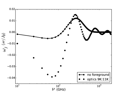
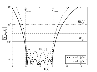
Figure 1: Results of the algorithm application when the foreground is an unknown superposition of graybody spectra with temperatures distributed in any possible way between 9 K and 11 K. We assume emissivity $\int\limits_{9K}^{11K}\mid a(T)\mid dT<10^{-3}$. Left panel: optimal weights $\omega_{j}$ for $\sigma=3$ $Jy/sr$. The points connected by the solid line show $\omega_{j}$ when there is no foreground. Right panel: maximum possible absolute value of the response to the foreground $R({\bf F})$ as functions of temperature for $\sigma=3$ $Jy/sr$ and $\sigma=1$ $Jy/sr$ shown in dashed and solid lines, correspondingly, assuming that all radiation is concentrated at one temperature $T$: $F(\nu)=10^{-3}\cdot B(\nu,T)$. Any combination of sources with different temperatures distributed between 9 K and 11 K with a restriction on $a(T)$ will give a response of less than $\frac{1}{(T_{max}-T_{min})}\int\limits_{T_{min}}^{T_{max}}\mid R({\bf F})\mid dT$. Horizontal dashed and solid lines represent the response to the noise. The horizontal dashed-dotted line is the response to the $\mu$ signal. Vertical lines limit the region of temperature variation.

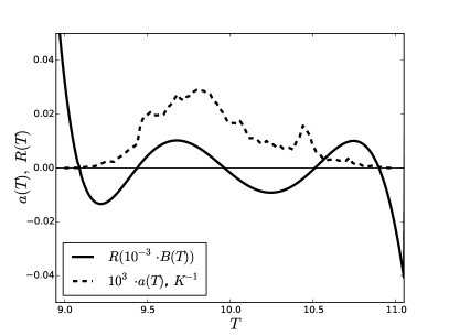
Figure 2: Simplified model of the foreground created by the telescope’s primary mirror. Left panel: simulated temperature distribution over the surface of the mirror in the experiment (Novikov et al., 2021). The gaps between the reflective panels have a slightly higher temperature than the panels themselves. Since the cooling machines are close to the center, the interior of the mirror is cooled more efficiently than the peripheral panels. The hot spot oriented at approximately 2 o’clock exists due to the corresponding orientation of the telescope relative to the Sun. This spot moves with time and makes a complete revolution around the mirror in one year. Right panel: amplitude distribution as a function of temperature $a(T)$ shown as a dashed line. The narrow peak at approximately 10.5 K corresponds to the contribution to the radiation from the gaps between the panels. The solid line shows the response to the graybody foreground when all radiation is concentrated at temperature $T$; i.e., $a(T)$ has the form of the delta function: $a(T^{\prime})=10^{-3}\cdot\delta(T^{\prime}-T)$ (same as in Fig. 1 for the photon noise $\sigma=1$ $Jy/sr$).

The simplest case is a problem with the foreground in the form of a superposition of graybody spectra:

$$\begin{array}[]{l}\vspace{0.2cm}I_{gb}(\nu)=\int\limits_{T_{min}}^{T_{max}}a(T)B(\nu,T)dT,\\ B(\nu,T)=\frac{2(kT)^{3}}{(hc)^{2}}\frac{x^{3}}{e^{x}-1},\hskip 5.69046ptx=\frac{h\nu}{kT},\end{array}$$ (16)

where $T_{min}:T_{max}$ is the range of possible temperature change from the minimum to the maximum value. This range plays the role of the $\Omega$ region in the case of a single parameter (temperature). One can always estimate (for example, for a telescope’s primary mirror) this range of temperature variations as well as the maximum possible value for the mirror emissivity function: $\int\limits_{T_{min}}^{T_{max}}\mid a(T)\mid dT<A_{max}$. The observed signal is

$$\begin{array}[]{l}\vspace{0.2cm}S_{j}=a_{\mu}I_{\mu}^{j}+\int\limits_{T_{min}}^{T_{max}}a(T)B_{j}(T)dT+N_{j},\\ B_{j}(T)=\int\limits_{{}_{\nu_{j}-\frac{\Delta\nu}{2}}}^{{}^{\nu_{j}+\frac{\Delta\nu}{2}}}B(\nu,T)\frac{d\nu}{\Delta\nu},\end{array}$$ (17)

For simplicity, we consider the covariance noise matrix to be a diagonal one.

In accordance with Eqs. (10) and (11), one can write an expression for the quadratic form $Q$:

$$\begin{array}[]{l}\vspace{0.2cm}Q=A_{max}^{2}\sum\limits_{i,j=1}^{J}q_{ij}\omega_{i}\omega_{j}+\sum\limits_{j=1}^{J}\sigma_{j}^{2}\omega_{j}^{2},\\ q_{ij}=\frac{1}{T_{max}-T_{min}}\int\limits_{{}_{T_{min}}}^{{}_{T_{max}}}B_{i}(T)B_{j}(T)dT.\\ \end{array}$$ (18)

Thus, Eqs. (12) and (18) give us weights $\omega_{j}$. If the amplitude of the noise greatly exceeds the possible contribution from the foreground, then the optimal weights will be $\omega_{j}\sim I_{\mu}^{j}/\sigma_{j}^{2}$ (as expected in the case of no foreground). For the noise uniformly distributed over all frequency channels ($\sigma_{j}=\sigma$), the weight function will have exactly the shape of the signal: $\omega_{j}\sim I_{\mu}^{j}$. By reducing the noise, we begin to significantly change the optimal values of the weights and thereby reduce not only the response to the noise $R({\bf N})$ but also the response to an unknown foreground signal $R({\bf F}(T))$. The response to a foreground is a function of $T$, while the response to noise is just a number.

In this numerical experiment the function $a(T)$ is random and unknown to us, but

$$\int\limits_{9K}^{11K}\mid a(T)\mid dT<A_{max}=10^{-3}.$$

The total number $J=128$ of frequency channels $\nu_{j}$ were used from 10 GHz to 2 THz with the channel width $\Delta\nu$=15 GHz. Figure 1 demonstrates the maximum possible response to the foreground $\mid R(10^{-3}\cdot{\bf B}(T))\mid>\mid R({\bf F}(T))\mid$ for two different values of photon noise, $\sigma$=3 Jy/sr and $\sigma$=1 Jy/sr. We can clearly see that for sufficiently small $\sigma=\langle N_{j}^{2}\rangle$, the optimally chosen coefficients $\omega_{j}$ provide a response to the foreground that is negligible compared to the response to the signal, $R({\bf I_{\bm{\mu}}})=1$.

Below we show an example of applying our algorithm to a real instrumental foreground created by telescope optics. Figure 2 (left panel) shows a simplified model of the primary telescope mirror in the experiment (Novikov et al., 2021). This model is a 10-meter-diameter mirror cooled to 10 K and consisting of 96 panels. Since the angular resolution is not a decisive factor in the study of $\mu$ distortions, such a large mirror is not necessary. Nevertheless, this experiment also involves the study of $y$ distortions and the effects associated with the scattering of relic photons on plasma in galaxy clusters (the SZ effect), where it is highly desirable to have a good resolution. This picture shows the temperature distribution over the surface of an unevenly cooled mirror. It is assumed that each surface element radiates as a graybody with temperature $T$ and emissivity less than $10^{-3}$. The surface temperature model of this mirror includes several terms:
$\bullet$ the average temperature T=10 K;
$\bullet$ the temperature gradient from the center to the periphery (due to the internal panels being cooled more efficiently);
$\bullet$ the hot spot due to one side of the telescope being heated by the Sun;
$\bullet$ a random Gaussian temperature distribution with a characteristic scale of cold and hot spots approximately corresponding to the size of the panels;
$\bullet$ the gaps between panels that are noticeably hotter than the rest of the surface.

The right panel of Fig. 2 shows the actual distribution of the amplitude $a(T)$ over temperature along with the response to the foreground when the amplitude is in the form of the delta function: $a(T^{\prime})=10^{-3}\cdot\delta(T^{\prime}-T)$, $R({\bf F})=R(10^{-3}\cdot{\bf B}(T))$ (the same as in Fig 1). Thus, the response to the actual foreground created by the mirror is

$$R({\bf F})=\int\limits_{9K}^{11K}a(T)R({\bf B}(T))dT.$$ (19)

In this particular case, the response $R({\bf F})=0.091\sigma_{{}_{F,max}}$ is very small compared to the estimated maximum possible variation. As noted above, the average value of the response to the foreground is not equal to zero. In order to find it we need to know the average distribution $\langle a(T)\rangle$:

$$\langle R({\bf F})\rangle=\int\limits_{9K}^{11K}\langle a(T)\rangle R({\bf B}(T))dT.$$ (20)

In our particular model we can assume that this average distribution does not differ much from the calculated $a(T)$ shown in Fig. 2. Thus, in real parameter distributions the bias is not only less than $\sigma_{{}_{F,max}}$ but, as a rule, it is significantly less than this overestimated variation. Since in the general case we do not know the properties of the function $a(T)$, we do not try to introduce any correction for the bias.

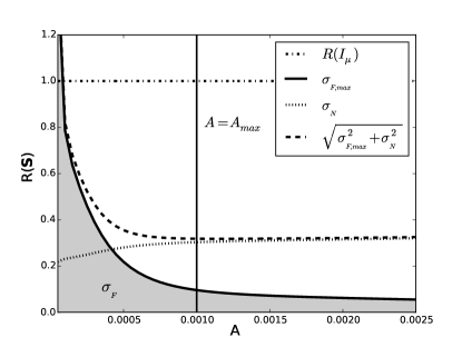
Figure 3: Dependence of $\sigma_{{}_{F}}$ and $\sigma_{{}_{N}}$ on the estimated upper limit $A=\int\mid a(T)\mid dT$ of the amplitude. Any combination of radiation sources in the form of a graybody with a temperature in the range from 9 K to 11 K and a total integrated amplitude less than $A$ will give a response $\mid R({\bf F})\mid$ that will be in the gray area below the line $\sigma_{{}_{F,max}}$. The minimum of the total deviation $\sqrt{\sigma_{{}_{F,max}}^{2}+\sigma_{{}_{N}}^{2}}$ is reached when the estimation of $A$ is correct: $A=A_{max}=10^{-3}$

In this simplified example, it is easy to see that modeling the spectrum emitted by the telescope optics is an extremely difficult (if not impossible) task. Any attempt to calculate such a spectrum (changing over the course of observations) is complicated by a large number of factors that must be taken into account. Our approach overcomes these difficulties. It is enough for us to know only three quantities: the minimum and maximum possible temperatures of the mirror surface, and its maximum possible emissivity. We also emphasize that the optics radiation must be modeled by a combination of modified blackbody radiation (the combination of graybody spectra is considered here for simplicity).

Figure 3 demonstrates how important it is to correctly estimate the upper limit of the amplitude $A_{max}$. It shows the dependence of $\sigma_{{}_{N}}$ and $\sigma_{{}_{F,max}}$ on the estimate of the upper limit of the amplitude $A$. Underestimation of this amplitude can lead to an increase in the response to the foreground and an incorrect interpretation of the data. At the same time, overestimation of this amplitude is not so risky in this case. Nevertheless, in more general cases an overestimation of the foreground amplitude can lead to a sharp increase in the response to photon noise, which reduces the accuracy of $a_{\mu}$ estimation. The minimum of the total deviation $\sqrt{\sigma_{{}_{N}}^{2}+\sigma_{{}_{F,max}}^{2}}$ of the response to the signal from the true amplitude $a_{\mu}$ is reached when $A=A_{max}$.

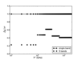
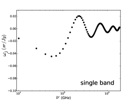
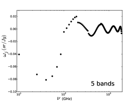
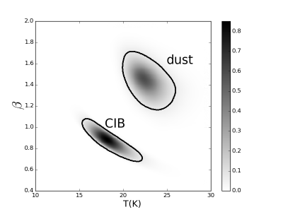
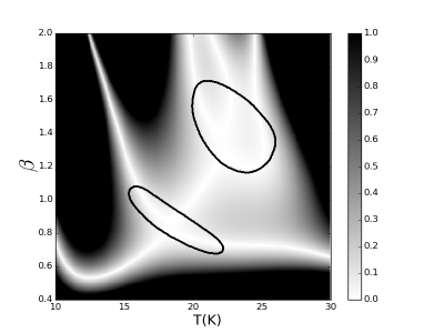
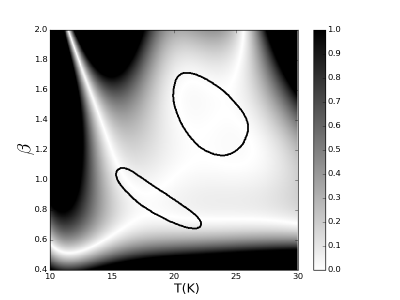
Figure 4: Separation of the $\mu$ signal from dust and CIB contamination. Top left: sensitivity for the frequency channels for one and five-band FTS. Bottom left: probability distribution function for parameters T and $\beta$ jointly for dust and infrared background. Top middle and top right: weights $\omega_{j}$ for single-band and five-band sensitivity, correspondingly. Bottom middle and bottom right: maximum possible foreground response $\mid R({\bf F}(T,\beta))\mid$, $\int\limits_{\Omega}\mid a(T,\beta)\mid dTd\beta<A_{max}=10^{-6}$ for dust+CIB for single-band and five-band FTS, correspondingly. Black color indicates the area where the response to the foreground is greater than the response to the signal: $\mid R({\bf F}(T,\beta))\mid>R({\bf I_{\bm{\mu}}})=1$. Bright white filamentlike lines correspond to geometric points in the $T,\beta$ coordinate plane where $R({\bf F}(T,\beta))=0$. The responses to the noise are $\sigma_{{}_{N}}=0.124$ and $\sigma_{{}_{N}}=0.046$ for one and five bands, respectively.

III.2 Dust and CIB foregrounds

As mentioned in the Introduction, dust and CIB contributions to the total signal can both be written in the following form:

$$I_{{}_{dust,CIB}}(\nu,T,\beta)=\tau(\nu/\nu_{0})^{\beta}B(\nu,T),$$ (21)

where the reference frequency $\nu_{0}$ of 353 GHz is used. Analogously to Eqs. (3) and (17), the total signal ${\bf S}=S_{1},..,S_{J}$ is

$$\begin{array}[]{l}\vspace{0.2cm}S_{j}=I_{\mu}^{j}+\int\limits_{\Omega}a(T,\beta)f(\nu_{j},T,\beta)dTd\beta+N_{j},\\ f(\nu_{j},T,\beta)=\int\limits_{{}_{\nu_{j}-\frac{\Delta\nu}{2}}}^{{}^{\nu_{j}+\frac{\Delta\nu}{2}}}(\nu/\nu_{0})^{\beta}B(\nu,T)\frac{d\nu}{\Delta\nu}.\end{array}$$ (22)

In order to determine the boundaries of the parameter $(T,\beta)$ domain, Planck data (Planck Collaboration et al., 2014, 2016) were used. The probability distribution function for these parameters was calculated using a 10-degree circular sky part centered at $l=13.731^{o}$, $b=-73.946^{o}$; see Fig. 4 (bottom left panel). The isocontour black lines limit the parameter region $\Omega(T,\beta)$. (Note that dust and CIB areas can, in principle, overlap. This does not change anything in our analysis since in this case we consider them as a single foreground.) The probability of finding parameters outside this region is less than 0.0002. At the same time, the maximum allowable value of emissivity $\tau$ for the data we used does not exceed $10^{-6}$: $\int\limits_{\Omega}\mid a(T,\beta)\mid dTd\beta<A_{max}=10^{-6}$. As in Sec. III A, 128 channels of 15 GHz width from 10 GHz to 2 THz were used. In order to compare the effectiveness of different FTS configurations, the results for two different cases are shown: single-band FTS and five-band FTS. Both of their sensitivities (noise $\langle N_{j}^{2}\rangle$) are calculated using (Benford et al., 1998; Lamarre, 1986) for the same integrating time (top left panel). Five-band FTS divides the frequency range into five isolated parts. Therefore, it is not surprising that it gives better sensitivity. The top middle panel and top right panel show results of calculating optimal weights $\omega_{j}$ for one and five bands, correspondingly. Unlike single-band weights, the weight function for five bands has discontinuities at points equal to the minimum and maximum frequencies of each band. Results for the maximum possible foreground response for these two cases are shown in the bottom middle and bottom right panels. It is clear that the five-band configuration provides us not only with a better noise response but also with a smaller and safer foreground response.

III.3 Other foregrounds

In the previous subsection the algorithm was applied to the case with dust and CIB. We now look at how other foregrounds can be included. First, we should add the radiation created by the optics of the telescope since it is described by the same modified blackbody formula and depends on the same parameters. In this case one more region is added to the two regions in the ${\bf P}=(T,\beta)$ plane in Fig. 4. This region corresponds to variations in temperature and spectral slope for the optical system. Its size and configuration depend on the properties of the primary mirror: average temperature, cooling system characteristics, the quality of surface grinding, etc. The next foregrounds to be added are the spectral distortions associated with the CMB radiation: CMB anisotropy (CMBA), SZ effect (y distortions), and its first relativistic correction (Challinor and Lasenby, 1998). (The CMB monopole spectrum is well known and can be subtracted from the total signal.) The most “harmful” is the CMBA:

$$\begin{array}[]{l}\vspace{0.2cm}I_{{}_{CMBA}}=\frac{2(kT_{0})^{3}}{(hc)^{2}}\frac{x^{4}}{(e^{x}-1)^{2}}\cdot\frac{\Delta T}{T_{0}},\\ x=h\nu/kT_{0},\end{array}$$ (23)

because its shape is exactly proportional to the first term in Eq. (1) for $\mu$ distortion. This is not surprising because CMBA and $\mu$ distortion have a similar physical origin. Therefore, particularly the second term in Eq. (1) gives us an opportunity to measure chemical potential. This term manifests itself mainly for $\nu<200$ GHz. Therefore, it is important to achieve good sensitivity at relatively low frequencies. As for the maximum possible CMBA amplitude, a safe estimate is $\mid\frac{\Delta T}{T_{0}}\mid<A_{{}_{CMBA}}=10^{-4}$. The shape of $I_{{}_{CMBA}}$ does not depend on any parameters ${\bf P}$, but formally, we consider this dependence to be a constant. Similarly, it is necessary to add the SZ effect and the first relativistic correction to it. The upper limit for their amplitudes depends on the specific position in the sky and the presence of strong SZ sources. Adding other foregrounds (synchrotron, free-free, etc.) with their floating parameters one by one, we finally get a complete set of components that must be taken into account when solving the problem of $\mu$ signal separation.

IV Conclusions

This paper presents a way to get rid of cosmic foregrounds with poorly defined spectral characteristics when measuring $\mu$ distortion. The basis of this approach is the algorithm for finding special weights for frequency channels. In the case of sufficient sensitivity, the sum of the signal measurements with these weights (called the response) is weakly sensitive to the presence of foregrounds with parameters lying in some preestimated range of their possible variations. Therefore, the response to the foregrounds becomes negligible in comparison with the response to the $\mu$ signal. In this paper only some types of foregrounds are considered. Applying the algorithm to all possible foregrounds is the subject of a separate detailed research.

It should be noted that this approach can be applied to experiments related to the study of phenomena associated with the SZ effect, for example Refs. (Novikov et al., 2020; Edigaryev et al., 2018; Challinor et al., 2000; Yasini and Pierpaoli, 2016; Shehzad Emritte et al., 2016; Itoh et al., 2000), as well as to any physical experiments with poorly defined foreground spectra.

We would like to thank the referee for helpful comments and a fruitful discussion.

This work is supported by Project No. 41-2020 of LPI’s new scientific groups and the Foundation for the Advancement of Theoretical Physics and Mathematics “BASIS,” Grant No. 19-1-1-46-1.

References

- Chluba et al. (2021) J. Chluba, M. H. Abitbol, N. Aghanim, Y. Ali-Haïmoud, M. Alvarez, K. Basu, B. Bolliet, C. Burigana, P. de Bernardis, J. Delabrouille, et al., Exp. Astron. 51, 1515 (2021).
- Chluba and Sunyaev (2012) J. Chluba and R. A. Sunyaev, Mon. Not. R. Astron. Soc 419, 1294 (2012).
- Silk and Chluba (2014) J. Silk and J. Chluba, Science 344, 586 (2014).
- De Zotti et al. (2016) G. De Zotti, M. Negrello, G. Castex, A. Lapi, and M. Bonato, J. Cosmol. Astropart. Phys. 047 (2016).
- Tashiro (2014) H. Tashiro, Prog. Theor. Exp. Phys. 2014, 06B107 (2014).
- Zeldovich and Sunyaev (1969) Y. B. Zeldovich and R. A. Sunyaev, Astrophys. Space. Sci 4, 301 (1969).
- Burigana et al. (1991) C. Burigana, L. Danese, and G. de Zotti, Astron. Astrophys 246, 49 (1991).
- Chluba et al. (2019) J. Chluba, A. Kogut, S. P. Patil, M. H. Abitbol, N. Aghanim, Y. Ali-Haımoud, M. A. Amin, J. Aumont, N. Bartolo, K. Basu, et al., Bull. Am. Astron. Soc. 51, 184 (2019).
- Nakama et al. (2018) T. Nakama, B. Carr, and J. Silk, Phys. Rev. D 97, 043525 (2018).
- Sunyaev and Zeldovich (1970a) R. A. Sunyaev and Y. B. Zeldovich, Astrophys. Space. Sci 7, 20 (1970a).
- Sunyaev and Zeldovich (1970b) R. A. Sunyaev and Y. B. Zeldovich, Astrophys. Space. Sci 9, 368 (1970b).
- Daly (1991) R. A. Daly, Astrophys. J 371, 14 (1991).
- Hu et al. (1994) W. Hu, D. Scott, and J. Silk, Astrophys. J., Lett 430, L5 (1994).
- Chluba et al. (2012) J. Chluba, R. Khatri, and R. A. Sunyaev, Mon. Not. R. Astron. Soc 425, 1129 (2012).
- Ota et al. (2014) A. Ota, T. Takahashi, H. Tashiro, and M. Yamaguchi, J. Cosmol. Astropart. Phys. 2014, 029 (2014).
- Kompaneets (1957) A. S. Kompaneets, Sov. J. Exp. Theor. Phys. 4, 730 (1957).
- Kogut et al. (2016) A. Kogut, J. Chluba, D. J. Fixsen, S. Meyer, and D. Spergel, in Space Telescopes and Instrumentation 2016: Optical, Infrared, and Millimeter Wave, edited by H. A. MacEwen, G. G. Fazio, M. Lystrup, N. Batalha, N. Siegler, and E. C. Tong (2016), vol. 9904 of Society of Photo-Optical Instrumentation Engineers (SPIE) Conference Series, p. 99040W.
- Novikov et al. (2021) I. D. Novikov, S. F. Likhachev, Y. A. Shchekinov, A. S. Andrianov, A. M. Baryshev, A. I. Vasyunin, D. Z. Wiebe, T. d. Graauw, A. G. Doroshkevich, I. I. Zinchenko, et al., Physics Uspekhi 64, 386 (2021).
- Abitbol et al. (2017) M. H. Abitbol, J. Chluba, J. C. Hill, and B. R. Johnson, Mon. Not. R. Astron. Soc 471, 1126 (2017).
- Chluba (2016) J. Chluba, Mon. Not. R. Astron. Soc 460, 227 (2016).
- Mukherjee et al. (2019) S. Mukherjee, J. Silk, and B. D. Wandelt, Phys. Rev. D 100, 103508 (2019).
- Miyamoto et al. (2014) K. Miyamoto, T. Sekiguchi, H. Tashiro, and S. Yokoyama, Phys. Rev. D 89, 063508 (2014).
- Kogut et al. (2011) A. Kogut, D. J. Fixsen, D. T. Chuss, J. Dotson, E. Dwek, M. Halpern, G. F. Hinshaw, S. M. Meyer, S. H. Moseley, M. D. Seiffert, et al., J. Cosmol. Astropart. Phys. 2011, 025 (2011).
- Pajer and Zaldarriaga (2012) E. Pajer and M. Zaldarriaga, Phys. Rev. Lett. 109, 021302 (2012).
- Ganc and Komatsu (2012) J. Ganc and E. Komatsu, Phys. Rev. D 86, 023518 (2012).
- Chluba et al. (2017) J. Chluba, J. C. Hill, and M. H. Abitbol, Mon. Not. R. Astron. Soc 472, 1195 (2017).
- Draine and Lee (1984) B. T. Draine and H. M. Lee, Astrophys. J 285, 89 (1984).
- Zelko and Finkbeiner (2021) I. A. Zelko and D. P. Finkbeiner, Astrophys. J 914, 68 (2021).
- Kogut and Fixsen (2016) A. Kogut and D. J. Fixsen, Astrophys. J 826, 101 (2016).
- Finkbeiner et al. (1999) D. P. Finkbeiner, M. Davis, and D. J. Schlegel, Astrophys. J 524, 867 (1999).
- Kirkpatrick et al. (2015) A. Kirkpatrick, A. Pope, A. Sajina, E. Roebuck, L. Yan, L. Armus, T. Díaz-Santos, and S. Stierwalt, Astrophys. J 814, 9 (2015).
- Mather et al. (1990) J. C. Mather, E. S. Cheng, J. Eplee, R. E., R. B. Isaacman, S. S. Meyer, R. A. Shafer, R. Weiss, E. L. Wright, C. L. Bennett, N. W. Boggess, et al., Astrophys. J., Lett 354, L37 (1990).
- Fixsen (2009) D. J. Fixsen, Astrophys. J 707, 916 (2009).
- Schutz (1999) B. F. Schutz, Classical and Quantum Gravity 16, A131 (1999).
- Owen and Sathyaprakash (1999) B. J. Owen and B. S. Sathyaprakash, Phys. Rev. D 60, 022002 (1999).
- Pitkin et al. (2011) M. Pitkin, S. Reid, S. Rowan, and J. Hough, Living Reviews in Relativity 14, 5 (2011).
- Zubeldia et al. (2021) Í. Zubeldia, A. Rotti, J. Chluba, and R. Battye, Mon. Not. R. Astron. Soc 507, 4852 (2021).
- Herranz et al. (2002) D. Herranz, J. L. Sanz, M. P. Hobson, R. B. Barreiro, J. M. Diego, E. Martínez-González, and A. N. Lasenby, Mon. Not. R. Astron. Soc 336, 1057 (2002).
- White and Padmanabhan (2017) M. White and N. Padmanabhan, Mon. Not. R. Astron. Soc 471, 1167 (2017).
- Zubeldia and Challinor (2019) Í. Zubeldia and A. Challinor, Mon. Not. R. Astron. Soc 489, 401 (2019).
- Planck Collaboration et al. (2014) Planck Collaboration, A. Abergel, P. A. R. Ade, N. Aghanim, M. I. R. Alves, G. Aniano, C. Armitage-Caplan, M. Arnaud, M. Ashdown, F. Atrio-Barandela, et al., Astron. Astrophys 571, A11 (2014).
- Planck Collaboration et al. (2016) Planck Collaboration, N. Aghanim, M. Ashdown, J. Aumont, C. Baccigalupi, M. Ballardini, A. J. Banday, R. B. Barreiro, N. Bartolo, S. Basak, et al., Astron. Astrophys 596, A109 (2016).
- Benford et al. (1998) D. J. Benford, T. R. Hunter, and T. G. Phillips, Int. J. Infrared Millim. Waves 19, 931 (1998).
- Lamarre (1986) J. M. Lamarre, Appl. Opt. 25, 870 (1986).
- Challinor and Lasenby (1998) A. Challinor and A. Lasenby, Astrophys. J 499, 1 (1998).
- Novikov et al. (2020) D. I. Novikov, S. V. Pilipenko, M. De Petris, G. Luzzi, and A. O. Mihalchenko, Phys. Rev. D 101, 123510 (2020).
- Edigaryev et al. (2018) I. G. Edigaryev, D. I. Novikov, and S. V. Pilipenko, Phys. Rev. D 98, 123513 (2018).
- Challinor et al. (2000) A. D. Challinor, M. T. Ford, and A. N. Lasenby, Mon. Not. R. Astron. Soc 312, 159 (2000).
- Yasini and Pierpaoli (2016) S. Yasini and E. Pierpaoli, Phys. Rev. D 94, 023513 (2016).
- Shehzad Emritte et al. (2016) M. Shehzad Emritte, S. Colafrancesco, and P. Marchegiani, J. Cosmol. Astropart. Phys. 031 (2016).
- Itoh et al. (2000) N. Itoh, S. Nozawa, and Y. Kohyama, Astrophys. J 533, 588 (2000).