Co-Salient Object Detection with Co-Representation Purification

Abstract

Co-salient object detection (Co-SOD) aims at discovering the common objects in a group of relevant images. Mining a co-representation is essential for locating co-salient objects. Unfortunately, the current Co-SOD method does not pay enough attention that the information not related to the co-salient object is included in the co-representation. Such irrelevant information in the co-representation interferes with its locating of co-salient objects. In this paper, we propose a Co-Representation Purification (CoRP) method aiming at searching noise-free co-representation. We search a few pixel-wise embeddings probably belonging to co-salient regions. These embeddings constitute our co-representation and guide our prediction. For obtaining purer co-representation, we use the prediction to iteratively reduce irrelevant embeddings in our co-representation. Experiments on three datasets demonstrate that our CoRP achieves state-of-the-art performances on the benchmark datasets. Our source code is available at https://github.com/ZZY816/CoRP.

1 Introduction

Human perception system [1] can effortlessly discover the most salient area. Co-salient object detection (Co-SOD) aims at discovering common salient objects from a group of relevant images. Meanwhile, Co-SOD needs to deal with unseen object categories, which are not learned during the training process. Such ability can serve as the preprocessing step for many real-world applications, e.g., video co-localization [2, 3], semantic segmentation [4], image quality assessment [5], and weakly supervised learning [6]. The difficulty of the Co-SOD task lies in discovering co-salient objects in the context of cluttered real-world environments. As shown in Fig. 1, it is challenging to automatically discover and segment the co-salient objects “banana” among multiple irrelevant salient objects.

To distinguish co-salient objects, most state-of-the-art (SOTA) methods directly estimate a co-representation to capture the shared characteristics of co-salient objects, by feature aggregation [7, 8], clustering [9, 10], principal component analysis [11, 12], global pooling [13, 14, 15], etc. The co-representations of these methods are summarized from all regions [13, 9, 11], or within pre-predicted salient regions [15, 16]. Although achieving promising performances in many scenes, they often ignore the noisy information related to irrelevant salient objects.

Utilizing noisy co-representation can lead to incorrect localization of co-salient objects, limiting Co-SOD models’ performances, especially for complex real-world scenes. To overcome this bottleneck, we try to reduce the irrelevant information in the co-representation. Unlike current methods directly obtaining the co-representation by summarizing all regions [13, 8, 9, 11] or salient regions [15, 16], we propose an iterative process to search confident locations only belonging to co-salient regions as our co-representation, which guides the complete segmentation of co-salient objects.

Specifically, we propose pure co-representation search (PCS) first to find confident embeddings belonging to co-salient regions as our co-representation. As shown in Fig. 1, among all pixel embeddings of salient objects, the embeddings of co-salient objects dominate because of the repetitiveness of co-salient objects in the image group. When obtaining the center by summarizing all the embeddings of salient regions, we find that the embeddings closer to the center are more likely to be of the co-salient ones. Based on this observation, instead of directly using the imperfect center to detect co-salient objects [15, 12], we treat the center as a proxy for indexing embeddings that have high correlation with it as co-representation. Compared with the proxy summarized from all the salient regions, our co-representation consisting of confident co-salient embeddings is less interfered by irrelevant noise.

\begin{overpic}[width=433.62pt]{./figures/main13.pdf} \put(38.0,-3.5){(a)} \put(78.0,-3.5){(b)} \put(23.0,5.5){{co-representation}} \put(41.0,38.0){{initial center}} \put(63.0,8.0){{new center}} \end{overpic}

Figure 1: t-SNE [17] visualization of embeddings. (a) “$\bullet$” represent embeddings of co-salient objects “banana”. We observe that the embeddings (in the blue circle area) quite near the center are very likely to belong to co-salient objects. We employ them as our co-representation to localize co-salient objects. (b) When many embeddings of irrelevant objects are filtered out by our primary prediction, we can obtain a new center less interfered by irrelevant embeddings. The new center helps search purer co-representation leading to more accurate prediction.

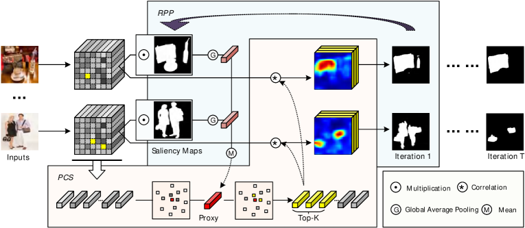
Figure 2: Overall framework of our CoRP. “PCS” and “RPP” denote the proposed pure co-representation search (Sec. 3.2) and recurrent proxy purification (Sec. 3.3). As shown above, when receiving a group of images, the corressponding saliency maps are firstly predicted by a backbone-shared saliency object detection (SOD) head. A co-representation proxy is generated upon filtering background noise by the saliency maps. With the help of the proxy, PCS searches pure co-representation, which guides co-saliency prediction. RPP feeds back co-saliency maps to calculate a new proxy, which helps searching purer co-representation. With the collaboration of PCS and RPP, the noise in the predictions is iteratively removed. For brevity, we do not draw our encoder-decoder architecture and the SOD head, which shares backbone parameters with this Co-SOD network.

Considering that the indexed co-representation from PCS still contains irrelevant embeddings, we propose recurrent proxy purification (RPP), using predicted co-saliency maps to purify the co-representation iteratively. After obtaining the prediction of co-salient maps, we use the prediction to filter out more noise and acquire a new proxy. The new proxy helps PCS search the co-representation with less noise for more accurate prediction. We carry out the above process iteratively to purify our co-representation. Under the alternate work of PCS and RPP, the irrelevant embeddings in our co-representation are gradually reduced. That is, the iteration process makes our representation purer and purer. We abbreviate our method as CoRP (Co-Representation Purification) in the following sections. In summary, our major contributions are given as follows.

• We propose two purification strategies: (i) PCS for minning noise-free co-representation and (ii) RPP for iteratively reducing noise based on the previous co-saliency maps.

• CoRP achieves SOTA performances on challenging datasets, CoCA [13], CoSOD3k [18], and CoSal2015 [19].

2 Related Works

Co-SOD by low-level consistency.  Since Jacobs et al. [20] firstly proposed the task of searching common salient objects among a series of relevant images, Co-SOD has been explored by the community for more than a decade. Early methods  [21, 2] focus on exploring the low-level consistency of co-salient objects in multiple images. Several methods  [7, 22] extract co-salient objects by gathering similar pixels across different images or common low-level cues from feature distributions. Other studies explore shared cues of a group of images by clustering [23], metric learning [24], or efficient manifold ranking [25]. Before searching inter-image repetitiveness, some other works [26, 21, 27] utilize the saliency maps of images to filter background noise to more accurately extract the co-salient objects.

Recently, multiple deep learning-based methods [28, 29, 19] have sprung up and significantly outperform previous traditional methods. These methods mainly focus on learning the co-representation of the image group and using it as a constraint signal for discovering the co-salient objects.

Co-SOD by deep consistency.  Wei et al. [8] concatenated a group of image features as the co-representation, and merged it back to each single image feature for automatic prediction. CSMG [11] applies a modified principal component analysis algorithm on image features to extract the co-representation used to generate prior masks. Zha et al. [9] compressed a group of features into a vector through the SVM classifier and regarded the vector as co-representation. GCAGC [10] generates co-attention maps through clustering and regards the cluster center as the co-representation. GICD [13] feeds each sample of the group images into a pre-trained classifier and sums up all the output as the co-representation. GCoNet [14] explores intra-group compactness and inter-group separability using the co-representation generated by group average pooling.

Co-SOD with salient regions refinements.  Some methods utilize saliency prediction to improve their performances. CoADNet [16] designs a group-wise channel shuffling for breaking the limit of the fixed input numbers. The shuffled features masked by saliency maps are concatenated together to obtain a co-representation. ICNet [15] weighted averages each feature masked by pre-predicted saliency maps as co-representation, which then be used to compare cosine similarity with each position for each sample. CoEGNet [12] employs a co-attention projection algorithm to extract the co-representation, which is utilized to generate co-attentions maps.

Exsiting methods mainly extract co-representations by directly discovering consistent representation using, e.g. clustering [23, 9, 10], principal component analysis [11, 12], metric learning [24], manifold ranking [25], or global pooling [13, 14, 15]. Even with salient region refinements, it is still difficult for these methods to avoid noisy co-representation associated with irrelevant salient objects.

\begin{overpic}[width=433.62pt]{./figures/analysis3.pdf} \put(1.5,28.0){Person} \put(51.4,29.0){Dolphin} \put(51.0,27.0){\&Person} \end{overpic}

Figure 3: Visualization of the locations of embeddings in our pure co-representation and the channels of feature $\mathbf{A}^{t}$ transformed by our pure co-representation. In the first row, each of the red point “$\bullet$” in one picture represents one of the top-$K$ spatial positions whose corresponding representation constitutes the pure co-representation. Each heatmap represents a channel of the converted feature (see Sec. 3.2). It is a correlation map calculated from the deep representation of the target image and the representation noted in the above red point.

Salient Object Detection.  Saliency object detection (SOD) aims at discovering regions that attract human visual attention in single images [30]. Traditional SOD methods [31, 32, 33, 34, 35] mainly rely on hand-crafted features to exploit low-level cues. Benefiting from the development of CNNs in segmentation tasks, many recent SOD methods [36, 37, 38, 39, 40, 41] design novel network architectures and make pixel-wise predictions.

Both SOD and Co-SOD are binary segmentation tasks, whose ground truth is binary masks. SOD provides several aspects of benefits for the Co-SOD studies. Co-SOD methods [15, 16] can employ single saliency maps to filter background noise and better localize co-salient objects. Meanwhile, the accurate single saliency maps can improve the ability of Co-SOD method [12] to segment object details. Further, after the jigsaw strategy was proposed by GICD [13], a large amount of SOD training data can be utilized to train Co-SOD models.

3 Proposed Method

3.1 Overview

Given a group of images $\mathcal{I}=\{\mathbf{I}_{n}\}_{n=1}^{N}$, co-saliency object detection aims to discover their commonly salient object(s) denoted by the co-saliency maps $\mathcal{M}=\{\mathbf{M}_{n}\}_{n=1}^{N}$. Our CoRP works with two key complementary purification procedures: Pure Co-representation Search (PCS) and Recurrent Proxy Purification (RPP). Our PCS is responsible for estimating co-representation with less irrelevant information and locating co-salient objects, while RPP utilizes predictions to further purify our co-representation.

As shown in Fig. 2, our PCS starts by extracting $\ell_{2}$-normalized deep representation $\mathcal{F}=\{\mathbf{F}_{n}\in\mathbb{R}^{D\times H\times W}\}_{n=1}^{N}$ for each sample in $\mathcal{I}$. For each of the $N\times H\times W$ spatial positions in the image group, there is a $D$ dimensional feature vector, either corresponding to the target common salient object(s) or the irrelevant foreground and background. Similar to [15, 12], we use saliency maps predicted by a backbone-shared SOD head as masks to pick feature vectors corresponding to potential common object regions, which are averaged to obtain a co-representation proxy $\boldsymbol{p}\in\mathbb{R}^{D}$. While this co-representation proxy contains rich information about the co-salient objects, the averaged representation $\boldsymbol{p}$ could easily contain irrelevant foreground information. Thus we try to search for a few most confident pixel-wise embeddings from the image features group for representing the common objects. More specifically, $K$ embeddings $\{\boldsymbol{c}_{k}\in\mathbb{R}^{D}\}_{k=1}^{K}$ from $\mathcal{F}$ are selected according to their distance to the co-representation proxy $\boldsymbol{p}$ as our co-representation $\mathbf{C}\in\mathbb{R}^{K\times D}$.

For obtaining purer co-representation $\mathbf{C}$, RPP utilizes our predicted co-saliency maps to purify our co-representation. To be specific, RPP feeds back existing prediction $\mathcal{M}$ to calculate more accurate co-representation proxy $\boldsymbol{p}$. With a new co-representation proxy, PCS can explore purer co-representation, which finally leads to better prediction. Our CoRP gradually eliminate the interference of background and extraneous foreground noise. We detail PCS and RPP in Sec. 3.2 and Sec. 3.3.

3.2 Pure Co-Representation Search (PCS)

Assume that we have obtained the co-representation proxy $\boldsymbol{p}^{t}\in\mathbb{R}^{D}$ of $t$-th iteration from RPP (see Sec. 3.3). Here, co-representation proxy $\boldsymbol{p}^{t}$ is a semantic embedding dominated by co-salient objects. Then, the group of deep representations $\mathcal{F}=\{\mathbf{F}_{n}\in\mathbb{R}^{D\times H\times W}\}_{n=1}^{N}$ contain $NHW$ pixel embeddings $\{\mathcal{F}^{(l)}\in\mathbb{R}^{D}\}_{l=1}^{NHW}$. From the pixel embeddings, PCS aims to find top-k embeddings $\{\boldsymbol{c}_{k}^{t}\in\mathbb{R}^{D}\}_{k=1}^{K}$, which are most correlated with the co-saliency dominated co-representation proxy $\boldsymbol{p}^{t}$. Concretely, we calculate the correlation score between each pixel embedding $\mathcal{F}^{(l)}\in\mathbb{R}^{D}$ and $\boldsymbol{p}^{t}$ by

$$\textit{Score}^{t(l)}=\boldsymbol{p}^{t}\mathcal{F}^{(l)\top}.$$ (1)

After sorting the scores in descending order, we record the spatial positions $\textit{Index}^{t}$ of the top-k embeddings with the highest correlation scores by

$$\textit{Index}^{t}=\arg\mathop{\text{topk}}_{l}{\left(\textit{Score}^{t(l)}\right)}\in\mathbb{R}^{K}.$$ (2)

According to the positions $\textit{Index}^{t}$, we gather the corresponding top-k embeddings from the $\mathcal{F}$ as our co-representation,

$$\mathbf{C}^{t}=\text{gather}\left(\mathcal{F},\textit{Index}^{t}\right)\in\mathbb{R}^{K\times D}.$$ (3)

Once obtaining co-representation $\mathbf{C}^{t}$, we preliminarily filter noise by co-representation proxy $\boldsymbol{p}^{t}$ and then transform each feature $\mathbf{F}_{n}$ in $\mathcal{F}$ to a set of correlation maps $\mathbf{A}_{n}\in\mathbb{R}^{K\times H\times W}$ by co-representation $\mathbf{C}^{t}$. Specifically,

$$\mathbf{\tilde{A}}_{n}^{t}=\mathbf{C}^{t}\left(\left(\boldsymbol{p}^{t}\mathbf{\tilde{F}}_{n}\right)\odot\mathbf{\tilde{F}}_{n}\right)\in\mathbb{R}^{K\times HW},$$ (4)

where $\mathbf{\tilde{F}}_{n}\in\mathbb{R}^{D\times HW}$ is reshaped from $\mathbf{F}_{n}\in\mathbb{R}^{D\times H\times W}$. We reshape the $\mathbf{\tilde{A}}^{t}_{n}\in\mathbb{R}^{K\times HW}$ to $\mathbf{A}^{t}_{n}\in\mathbb{R}^{K\times H\times W}$. then we get $\mathcal{A}^{t}=\{\mathbf{A}^{t}_{n}\}^{N}$ for the group of images. Finally, we decode $\mathcal{A}^{t}$ to predict the co-saliency maps $\mathcal{M}^{t}$.

Further, we explain the transformed feature $\mathcal{A}$ in detail. Each $\mathbf{A}^{t}_{n}\in\mathbb{R}^{K\times H\times W}$ in $\mathcal{A}^{t}$ can be regards as $K$ correlation maps calculated with $K$ embeddings $\{\boldsymbol{c}_{k}^{t}\in\mathbb{R}^{D}\}_{k=1}^{K}$ of our co-representation $\mathbf{C}^{t}$. In Fig. 3, we visualize some correlation maps and the locations (noted by “red point” ) of their corresponding embeddings. This transformed feature $\mathbf{A}^{t}_{n}$ brings three advantages according to the three observations below.

1) Sparse locations falls in the correct regions of co-salient objects. It means our co-representation $\mathbf{C}^{t}$ compose of the embeddings $\{\boldsymbol{c}_{k}^{t}\}_{k=1}^{K}$ extracted from the semantic embeddings belonging to co-salient objects. That is why our co-representation is purer than current methods which aggregate information from all locations;

2) Different embedding vectors $\boldsymbol{c}_{k}^{t}$ focus on different regions of co-salient objects. As the first example (person) in Fig. 3, the vectors extracted from the people’s heads, chest, and legs give more activation to the corresponding regions of the target people. Similarly, in the second group (person and dolphin), the vectors of dolphins and the vectors of people, respectively activate the regions of the two kinds of objects. Overall, the vectors $\boldsymbol{c}_{k}^{t}$ learn the information of the co-salient objects. For each vector, the information it learns is related to the position where it is exacted from. This diversity helps CoRP predict a more comprehensive target object regions;

3) Semantic feature $\mathbf{F}_{n}$ converts to a concatenated correlation maps $\mathbf{A}^{t}_{n}$, which is generated only from the correlation of intra group representation. This conversion makes our CoRP focus on discovering intra group connections, rather than fitting the semantic categories of the training set. All these advantages make our model obtain better predictions. We will further corroborate this in the ablation studies.

\begin{overpic}[width=433.62pt]{./figures/vis_iters.pdf} \put(8.8,-2.5){Iteration 1} \put(42.3,-2.5){Iteration 2} \put(76.0,-2.5){Iteration 3} \end{overpic}

Figure 4: Distribution of the obtained co-representation proxies and corresponding ground-truth ones in different iterations. We visualize all 80 groups in CoCA [13] by $t$-SNE [17] algorithm. Here, the blue triangle “$\blacktriangle$” means the co-representation proxies masked-averaged by co-saliency maps, and the orange square “$\blacksquare$” denotes the pure co-representation proxies masked-averaged by ground-truth maps. The result shows that the iteration process makes the co-representation proxies approach the ground-truth ones gradually.

\begin{overpic}[width=433.62pt]{./figures/recurrent_img_v2.pdf} \put(5.0,-4.0){Input} \put(21.0,-4.0){Iteration1} \put(41.0,-4.0){Iteration2} \put(62.0,-4.0){Iteration3} \put(87.0,-4.0){GT} \end{overpic}

Figure 5: Predicitons in different iterations. We can see that the predictions are gradually approaching the ground-truth labels. It is thanks to the gradually purified co-representation in the iteration. Note that the predictions with less foreground noise are conducive to mine purer co-representation.

3.3 Recurrent Proxy Purification (RPP)

RPP calculates co-representation proxy $\boldsymbol{p}^{t}\in\mathbb{R}^{D}$ based on the predicted co-saliency map $\mathcal{M}^{t-1}=\{\mathbf{M}^{t-1}_{n}\}_{n=1}^{N}$ in the last iteration. $\mathcal{M}^{0}$ is initialized by our SOD head which shares backbone features with our Co-SOD network. The details of the SOD head will be explained in Sec. 4.1. As co-salient object(s) recurs in every sample, the semantic representation masked by $\mathcal{M}^{t-1}$ are domainated by the embeddings of co-salient object(s). In this way, we directly average the spatial locations highlighted by $\mathcal{M}^{t-1}$ of $\mathcal{F}$ as the co-representation proxy $\boldsymbol{p}^{t}$,

$$\boldsymbol{p}^{t}=\sum_{n=1}^{N}\frac{\mathtt{GAP}(\mathbf{M}^{t-1}_{n}\odot\mathbf{F}_{n})}{N}\in\mathbb{R}^{D},$$ (5)

where $\odot$ denotes element-wise production, and the global average pooling (GAP) can be formalized as $\mathtt{GAP}(\mathbf{F})=\frac{1}{HW}\sum_{i}\sum_{j}\mathbf{F}$, in which $i=1,...,W$ and $j=1,...,H$. Again, $\boldsymbol{p}^{t}$ is normalized with Euclidean distance.

Note that $\boldsymbol{p}^{t}$ helps PCS predict more noise-free $\mathcal{M}^{t}$ compared with $\mathcal{M}^{t-1}$. In turn, the $\mathcal{M}^{t}$ makes RPP generate $\boldsymbol{p}^{t+1}$ with less noise compared with $\boldsymbol{p}^{t}$. Working with pure co-representation search (PCS), recurrent proxy purification (RPP) makes our CoRP iterative like

$$\left\{\begin{array}[]{rl}\boldsymbol{p}^{t}&=\text{RPP}\left(\mathcal{M}^{t-1},\mathcal{F}\right)\\ \mathcal{M}^{t}&=\text{PCS}\left(\boldsymbol{p}^{t},\mathcal{F}\right)\end{array}\right.,t=\{1,2,3,...,T\}.$$ (6)

Besides, we just utilize the encoder of our model for one time and the encoder does not paticipate in the following iteration process. In other words, our RPP makes PCS and the decoder works repeatly without encoder. In this case, the iteration process does not increase much computational burden. We details the iterative process in Algorithm 1.

Input: A group of images $\mathcal{I}=\{\mathbf{I}_{n}\}_{n=1}^{N}$

Output: Co-saliency maps $\mathcal{M}^{T}=\{\mathbf{M}^{T}_{n}\}_{n=1}^{N}$

Initialize: Extract deep representation $\mathcal{F}=\{\mathbf{F}_{n}\}_{n=1}^{N}$; initilize $\mathcal{M}^{0}$ with our backbone-shared SOD head

for $t\leftarrow 1$ to $T$ do

       RPP

             Generate co-representation proxy $\boldsymbol{p}^{t}$ based on $\mathcal{F}$ and $\mathcal{M}^{t-1}$ (Eq. 5)

       end

      

      PCS

             Obtain $\textit{Score}^{t}$ by scoring each spatial location in $\mathcal{F}$ with $\boldsymbol{p}^{t}$ (Eq. 1)

            Search top-k purer embeddings as co-representation $\mathbf{C}^{t}$ from $\mathcal{F}$ based on $\textit{Score}^{t}$ (Eq. 2, 3)

            Transform each $\mathbf{F}_{n}$ to a set of correlation maps $\mathbf{A}^{t}_{n}$ with co-representation $\mathbf{C}^{t}$ (Eq. 4), then obtain $\mathcal{A}^{t}=\{\mathbf{A}^{t}_{n}\}^{N}$

            Predict $\mathcal{M}^{t}=\{\mathbf{M}^{t}_{n}\}_{n=1}^{N}$ by decoding $\mathcal{A}^{t}$

       end

      

end for

Algorithm 1 Co-Salient Object Detection with Co-Representation Purification

To better understand what happened in the iteration, we analyze the changes of three important factors.

1) Co-representation proxy gradually approaches that obtained by ground-truth annotation. In Fig. 4, we visualize the co-representation proxies of all 80 groups in CoCA [13] by $t$-SNE. In each iteration, we denote the proxies masked-averaged by co-saliency maps as “blue triangle”, and these masked-averaged by ground-truth annotation as “orange square”. With the co-saliency maps are gradually predicted accuracy, the distance between the two kinds of proxies gradually shrinks. As the orange nodes denote noise-free proxies completely generated by embeddings belonging to co-saliency objects, the reduction of the distance means our RPP gradually reduces the distracting information in our proxies.

2) Co-representation consists of more and more repesenations from co-salient regions. In Tab. I, we count the proportion of the space-wise position of the embeddings falling on the co-salient object. On the three benchmark datasets, the average proportions grow after each iteration. After three-times of iteration, more than two-thirds of embeddings in the co-representations are located at co-salient objects. The growth of proportions means the co-representations contain more co-saliency information and less distracting noise. Due to the reduction of distracting information in the proxy, the co-representation is gradually purified with the iterative process.

3) Co-saliency maps gradually eliminate the background and irrelevant foreground objects. We show the predicted results in Fig. 5. In the first iteration, background interference is suppressed, but it still contains much foreground noise, which fades away during further interations guided by purer co-representation.

Table I: Proportion of the sparse locations for extracting co-representation falling on the co-salient objects. With the iterative process, co-representation extracts more from the corresponding feature positions of co-salient objects; thus, our co-representation becomes purer and purer.

	CoCA [13]	CoSal2015 [19]	CoSOD3k [18]
$T$ = 1	60.3%	93.2%	82.4%
$T$ = 2	65.3%	94.6%	84.8%
$T$ = 3	66.8%	94.9%	85.1%
$T$ = 4	67.2%	95.0%	85.2%
$T$ = 5	67.3%	95.0%	85.3%
$T$ = 6	67.3%	95.0%	85.3%

4 Experiment

4.1 Implementation Details

Model details.  We employ pretrained VGG-16 [42] as our backbone and construct an encoder-decoder architecture. In CoRP, the initial saliency map $\mathcal{M}^{0}$ is predicted by our backbone-shared SOD head. After acquiring the first co-representation proxy $\boldsymbol{p}^{1}$ with $\mathcal{M}^{0}$, we employ our PCS on the last four outputs of the encoder. PCS aims at localizing co-saliency objects and produces four co-saliency features. Our decoder, which is the same as that of ICNet [15] decodes the four co-saliency features and remaining shallow features to predict co-saliency maps $\mathcal{M}^{1}$. Our RPP feeds back $\mathcal{M}^{1}$ to produce a new co-representation proxy and repeat the process just mentioned to predict $\mathcal{M}^{2}$. The iteration process produces $\{\mathcal{M}^{1},\mathcal{M}^{2},\mathcal{M}^{3},...,\mathcal{M}^{T}\}$ and we set $T=3$ in our experiments. The reason will be explained in Sec. 4.4.

The SOD head, which produces initial saliency maps $\mathcal{M}^{0}$ shares backbone weights with our CoSOD network. The decoder of the SOD head is designed independently and directly merges the outputs of the encoder and predict saliency maps. The SOD head adds 2.9 MB of model parameters to our CoRP.

Table II: Quantitative comparisons of mean absolute error ($MAE$), maximum F-measure [43] ($F_{\max}$), S-measure [44] ($S_{\alpha}$), and mean E-measure [45] ($E_{\xi}$) by our CoRP and other methods on the CoCA [13], CoSOD3k [18], and CoSal2015 [19] datasets. DUTS-Class [13], COCO-9k [8], COCO-SEG [9], and MSRA-B [46] are wildly used training datasets in Co-SOD and we denote them as Train-1, 2, 3, and 4, respectively. “$\uparrow$” means that the higher the numerical value, the better the model performance. The numerical value with an underline refers to the second best result under VGG16 backbone. Specifically, our CoRP shows the results in the third iteration ($T$ = 3). We provide the performances of our model with three backbones: VGG16[42], ResNet50 [47] and PVTv1-medium [48]. CoRP${}^{\text{NAS}}$ represents that we find the optimal hyper parameter K in our PCS by Network Architecture Search [49].

		GateNet	GCPA	CBCD	CSMG	GCAGC	GICD	ICNet	CoEG	DeepACG	GCoNet	CADC	CoRP	CoRP	CoRP${}^{\text{{\color[rgb]{0,0,0}NAS}}}$	CoRP	CoRP
		ECCV20	AAAI20	TIP13	CVPR19	CVPR20	ECCV20	NeurIPS20	TPAMI21	CVPR21	CVPR21	ICCV21	2021	2021	2021	2021	2021
		[50]	[51]	[23]	[11]	[10]	[13]	[15]	[12]	[52]	[14]	[53]	VGG16	VGG16	VGG16	Res-50	PVT
	Training Set	-	-	-	Train-4	Train-3	Train-1	Train-1,2	Train-1	Train-3	Train-1	Train-1,2	Train-2	Train-1,2	Train-1,2	Train-1,2	Train-1,2
	MAE$\downarrow$	0.097	0.082	0.233	0.130	0.085	0.071	0.058	0.078	0.064	0.068	0.064	0.060	0.049	0.049	0.046	0.044
	$F_{\max}\uparrow$	0.772	0.830	0.547	0.787	0.832	0.844	0.859	0.836	0.842	0.847	0.862	0.864	0.885	0.888	0.893	0.895
	$S_{\alpha}\uparrow$	0.811	0.850	0.550	0.776	0.823	0.844	0.855	0.838	0.854	0.845	0.866	0.859	0.875	0.877	0.879	0.884
CoSal2015	$E_{\xi}\uparrow$	0.820	0.864	0.516	0.763	0.814	0.883	0.896	0.868	-	0.884	-	0.896	0.913	0.915	0.919	0.920
	MAE$\downarrow$	0.173	0.188	0.180	0.114	0.111	0.126	0.148	0.106	0.102	0.105	0.132	0.101	0.121	0.110	0.104	0.093
	$F_{\max}\uparrow$	0.398	0.435	0.313	0.499	0.517	0.513	0.514	0.493	0.552	0.544	0.548	0.564	0.551	0.575	0.607	0.619
	$S_{\alpha}\uparrow$	0.600	0.612	0.523	0.627	0.666	0.658	0.657	0.612	0.688	0.673	0.681	0.699	0.686	0.703	0.719	0.732
CoCA	$E_{\xi}\uparrow$	0.609	0.612	0.535	0.606	0.668	0.701	0.686	0.679	-	0.739	-	0.750	0.715	0.741	0.745	0.773
	MAE$\downarrow$	0.112	0.104	0.228	0.157	0.100	0.079	0.097	0.084	0.089	0.071	0.076	0.067	0.075	0.072	0.057	0.057
	$F_{\max}\uparrow$	0.697	0.746	0.468	0.730	0.779	0.770	0.766	0.758	0.756	0.777	0.759	0.794	0.798	0.801	0.828	0.835
	$S_{\alpha}\uparrow$	0.763	0.795	0.529	0.727	0.798	0.797	0.798	0.778	0.792	0.802	0.801	0.820	0.820	0.825	0.842	0.850
CoSOD3k	$E_{\xi}\uparrow$	0.772	0.813	0.509	0.675	0.791	0.845	0.843	0.817	-	0.857	-	0.864	0.862	0.866	0.887	0.891

Training details.  Following [15], the datasets we use for training our co-saliency model (CoRP) are DUTS dataset [54] and a subset of COCO dataset [55], containing 9213 images. The Co-SOD network is trained with the subset of COCO [55] while the backbone shared SOD head is trained together with DUTS dataset [54]. The Adam optimizer is used with an initial learning rate of $1\times 10^{-5}$ and a weight decay of $1\times 10^{-4}$. We train our model for 70 epochs in total. It takes about 4.5 hours on an Nvidia Titan X. In each training iteration, we randomly select 10 samples as a batch from an image group of COCO [55] subset to train the Co-SOD network and 8 samples from DUTS [54] to train SOD head. At testing stage, each batch is made up of all images within a Co-SOD group, and images from SOD datasets are not required. At both training and test stages, the images are resized into $224\times 224$, and we augment the data by randomly flip images horizontally at the training stage. Finally, the predictions are resized back for evaluation. Our CoRP is implemented in PyTorch [56] and Jittor [57]. The PyTorch version runs at 45.3 FPS with total parameters size of 80.1 MB on an Nvidia Titan X GPU when the number of iterations is set to three ($T$=3).

At training stage, we use the ground truth as mask to generate a noise-free co-representation proxy. With a completely noise-free proxy, our PCS locate co-saliency objects accurately and this training strategy makes our Co-SOD network fully rely on PCS to locate objects. In this way, our RPP is not employed at training stage. At testing stage, the first co-representation proxy is initialized by saliency maps produced by our SOD head. At the same time, RPP iteratively feeds predicted co-saliency maps into PCS, which provides more accurate objects localization and finally generates more accurate co-saliency maps. The iteration times of RPP can be set freely at testing stage, and we will discuss it in Sec. 4.4.

\begin{overpic}[width=433.62pt]{./figures/compare_map.pdf} \put(14.2,65.0){\color[rgb]{1,1,1}{CoSal2015}} \put(47.5,65.0){\color[rgb]{1,1,1}{CoSOD3k }} \put(81.1,65.0){\color[rgb]{1,1,1}{CoCA }} \put(1.7,58.7){\scriptsize{\rotatebox{90.0}{Input}}} \put(1.7,52.7){\scriptsize{\rotatebox{90.0}{GT}}} \put(1.7,46.0){\scriptsize{\rotatebox{90.0}{CoRP}}} \put(1.7,39.0){\scriptsize{\rotatebox{90.0}{GCoNet}}} \put(1.7,33.0){\scriptsize{\rotatebox{90.0}{CoEG}}} \put(1.7,26.9){\scriptsize{\rotatebox{90.0}{ICNet}}} \put(1.7,20.5){\scriptsize{\rotatebox{90.0}{GICD}}} \put(1.7,13.3){\scriptsize{\rotatebox{90.0}{GCAGC}}} \put(1.7,7.5){\scriptsize{\rotatebox{90.0}{CSMG}}} \put(1.7,1.0){\scriptsize{\rotatebox{90.0}{CBCD}}} \end{overpic}

Figure 6: Visual comparison of our CoRP with six SOTA methods. We demonstrate the predictions from three categories (lemon, chime, and binoculars) belonging to the three benchmark dataset (CoSal2015 [19], CoSOD3k [18], and CoCA [13]). We highlight the results of CoRP with an orange frame.

Table III: Ablation study of the proposed CoRP on the CoCA and CoSOD3k datasets. “SOD” refers to our SOD head which share backbone weights with our Co-SOD network. “PCS” and “RPP” are the proposed pure co-representation search and recurrent proxy purification. “baseline” refers to our Co-SOD encoder-decoder architecture without “SOD”, “PCS” and “RPP”. “baseline + SOD + proxy” denotes using directly the proxy as co-representation.

ID	Combination	CoCA [13]				CoSal2015 [19]				CoSOD3k [18]
		$F_{\text{avg}}\uparrow$	$F_{\max}\uparrow$	$S_{\alpha}\uparrow$	$E_{\xi}\uparrow$	$F_{\text{avg}}\uparrow$	$F_{\max}\uparrow$	$S_{\alpha}\uparrow$	$E_{\xi}\uparrow$	$F_{\text{avg}}\uparrow$	$F_{\max}\uparrow$	$S_{\alpha}\uparrow$	$E_{\xi}\uparrow$
1	baseline	0.381	0.397	0.560	0.563	0.652	0.662	0.699	0.727	0.576	0.590	0.654	0.687
2	baseline + SOD	0.436	0.443	0.608	0.640	0.760	0.772	0.800	0.830	0.688	0.697	0.753	0.795
3	baseline + SOD + proxy	0.381	0.399	0.551	0.531	0.798	0.825	0.836	0.866	0.675	0.697	0.744	0.766
4	baseline + SOD + PCS	0.474	0.488	0.640	0.658	0.860	0.874	0.869	0.906	0.753	0.764	0.800	0.839
CoRP	baseline + SOD + PCS + RPP	0.541	0.551	0.686	0.715	0.872	0.885	0.875	0.913	0.788	0.798	0.820	0.862

Loss function.  We take the IoU loss [58] for training our CoRP. The IoU loss has been proved to be effective for Co-SOD task in [13, 15]. Its specific formula is as follows:

$$\text{L}(\mathcal{M},\mathcal{G})\!=\!1\!-\!\sum_{n=1}^{N}\frac{\sum_{w=1}^{W}\sum_{h=1}^{H}\text{min}\{\mathbf{M}^{w,h}_{n},\mathbf{G}^{w,h}_{n}\}}{\sum_{w=1}^{W}\sum_{h=1}^{H}\text{max}\{\mathbf{M}^{w,h}_{n},\mathbf{G}^{w,h}_{n}\}}.$$ (7)

$\mathcal{M}=\{\mathbf{M}_{n}\}_{n=1}^{N}$ and $\mathcal{G}=\{\mathbf{G}_{n}\}_{n=1}^{N}$ represents the co-saliency maps generated by our model and the ground truth respectively. $\mathbf{M}^{w,h}_{n}$ denotes a pixel position of the $n$-th co-saliency map $\mathbf{M}_{n}$ in a group of predictions, and so does $\mathbf{G}^{w,h}_{n}$ in the corresponding group of ground truth.

To supervise our SOD head, we use $\mathcal{S}=\{\mathbf{S}_{m}\}_{m=1}^{M}$ and $\mathcal{T}=\{\mathbf{T}_{m}\}_{m=1}^{M}$ to represent the predicted saliency maps and the corresponding ground truth. We also employ IoU loss $\text{L}(\mathcal{S},\mathcal{T})$ for the SOD head. Our final loss function for training both Co-SOD network and SOD head simultaneously is as follows:

$$\text{L}_{all}=\alpha\text{L}(\mathcal{M},\mathcal{G})+\beta\text{L}(\mathcal{S},\mathcal{T}),$$ (8)

where we set $\alpha=0.8$ and $\beta=0.2$.

4.2 Evaluation Datasets and Metrics

Datasets.  We evaluate our CoRP on three challenging datasets: CoSal2015 [19], CoSOD3k [18], and CoCA [13]. The three datasets are widely used in evaluating Co-SOD methods. Cosal2015 [19] contains 2015 images of 50 categories, and each group has one or more challenging issues such as complex environments, object appearance variations, occlusion, and background clutters. CoSOD3k [18] is the largest CoSOD evaluation dataset so far, which covers 13 super-classes and contains 160 groups and totally 3,316 images. Each group includes diverse realistic scenes, and different object appearances, and covers the major challenges in CoSOD. CoCA [13] dataset consists of 80 categories with 1295 images Compared with Cosal2015 and CoSOD3k, CoCA has two special characteristics. Firstly, every image contains extraneous salient objects except for co-salient objects. Meanwhile, the image groups in CoCA [13] dataset are entirely unseen categories for our CoRP because CoCA does not have the same category as our training set. Thanks to these two key factors, the results on CoCA can better reflect the performance of each method on the class-agnostic Co-SOD task.

Metrics.  Following GICD [13], we report four widely used metrics, namely mean absolute error (MAE), maximum F-measure ($F_{\max}$) [43], S-measure ($S_{\alpha}$) [44], and mean E-measure ($E_{\xi}$). The evaluation code is available at https://github.com/zzhanghub/eval-co-sod.

4.3 Comparison with Current Methods

To illustrate the performance of our CoRP, we compare our method with nine SOTA Co-SOD methods, including CBCD [23], CSMG [11], GCAGC [10], GICD [13], CoEG-Net [12], ICNet [15], DeepACG [52], GCoNet [14], and CADC [53]. Meanwhile, following [13, 15, 16], we also report the result of two SOTA SOD methods, namely GateNet [50] and GCPA [51], as baselines.

Quantitative evaluation..  In Tab. II, we compare our method CoRP with other SOTA Co-SOD and SOD methods in quantitative results. We can see that our CoRP achieves SOTA performances across the three benchmark datasets. On CoCA [13] dataset, the performance of our method surpasses the others to a great degree in terms of max F-measure and S-measure. Compared with the second-best methods on CoCA [13] dataset, our method CoRP lead them by 1.5% in terms of S-measure and 2.3% in terms of max F-measure. As there are extraneous salient objects except for co-salient objects in each image of CoCA, our outperformance shows that our method has a better capacity for localizing co-salient objects. Meanwhile, CoCA [13] does not contain any image category which appears in our training dataset COCO [55]. Our leading performance on this dataset demonstrates that our method is robust to the unseen class in the class-agnostic task. Noticing that the performance of SOD methods, especially GCPANet [51], is comparable to or even better than some Co-SOD methods on CoSOD3k [18] and CoSal2015 [19] datasets because a large part of images in these two datasets contain only one salient object. However, our method also surpasses the second-best Co-SOD methods on CoSal2015 [19] and CoSOD3k [18] by 1.1% and 2.3% in terms of S-measure. Our performance on the three benchmark datasets fully demonstrates our method’s effectiveness. In addition, our method does not outperform all the others in terms of MAE. This may be due to the insufficient capacity of our method to segment object details.

Qualitative result..  In Fig. 6, we compare the our method’s predictions with other methods on the three benchmark datasets. Our method successfully separates the lemons from other parts of the images, while some other methods fail to distinguish the bananas from the lemons. Although the images of chime have complex background with great change, our method localizes the chimes and separates them from the background accurately. Meanwhile, the hands on the binocular are tiny but our method can separate the binoculars from the hands.

\begin{overpic}[width=433.62pt]{./figures/categories3.pdf} \put(3.2,24.5){\scriptsize{\rotatebox{90.0}{hammer}}} \put(5.2,23.7){\scriptsize{\rotatebox{90.0}{pineapple}}} \put(7.2,23.1){\scriptsize{\rotatebox{90.0}{frenchhorn}}} \put(9.2,26.0){\scriptsize{\rotatebox{90.0}{piano}}} \put(11.2,24.5){\scriptsize{\rotatebox{90.0}{baseball}}} \put(13.2,27.0){\scriptsize{\rotatebox{90.0}{axe}}} \put(14.9,25.7){\scriptsize{\rotatebox{90.0}{guitar}}} \put(16.9,23.3){\scriptsize{\rotatebox{90.0}{motorbike}}} \put(18.8,24.2){\scriptsize{\rotatebox{90.0}{babycrib}}} \put(20.8,22.6){\scriptsize{\rotatebox{90.0}{billiardtable}}} \put(22.8,23.2){\scriptsize{\rotatebox{90.0}{mushroom}}} \put(24.8,23.6){\scriptsize{\rotatebox{90.0}{coffeecup}}} \put(26.8,25.4){\scriptsize{\rotatebox{90.0}{mouse}}} \put(28.5,26.5){\scriptsize{\rotatebox{90.0}{train}}} \put(30.5,25.2){\scriptsize{\rotatebox{90.0}{helmet}}} \put(32.4,25.8){\scriptsize{\rotatebox{90.0}{lizard}}} \put(34.4,25.1){\scriptsize{\rotatebox{90.0}{banana}}} \put(36.2,24.4){\scriptsize{\rotatebox{90.0}{ladybird}}} \put(38.2,26.7){\scriptsize{\rotatebox{90.0}{bird}}} \put(40.1,27.2){\scriptsize{\rotatebox{90.0}{cat}}} \put(42.1,23.2){\scriptsize{\rotatebox{90.0}{goldenfish}}} \put(44.1,26.1){\scriptsize{\rotatebox{90.0}{viola}}} \put(45.9,26.4){\scriptsize{\rotatebox{90.0}{tiger}}} \put(47.9,25.6){\scriptsize{\rotatebox{90.0}{chook}}} \put(49.9,23.2){\scriptsize{\rotatebox{90.0}{mobulidae}}} \put(51.8,26.4){\scriptsize{\rotatebox{90.0}{snail}}} \put(53.8,26.6){\scriptsize{\rotatebox{90.0}{sofa}}} \put(55.8,26.3){\scriptsize{\rotatebox{90.0}{bowl}}} \put(57.7,26.6){\scriptsize{\rotatebox{90.0}{boat}}} \put(59.6,26.0){\scriptsize{\rotatebox{90.0}{horse}}} \put(61.6,25.5){\scriptsize{\rotatebox{90.0}{lemon}}} \put(63.6,25.8){\scriptsize{\rotatebox{90.0}{snake}}} \put(65.4,23.7){\scriptsize{\rotatebox{90.0}{aeroplane}}} \put(67.4,26.7){\scriptsize{\rotatebox{90.0}{frog}}} \put(69.4,25.8){\scriptsize{\rotatebox{90.0}{rabbit}}} \put(71.2,26.1){\scriptsize{\rotatebox{90.0}{turtle}}} \put(73.2,25.3){\scriptsize{\rotatebox{90.0}{pepper}}} \put(75.0,24.6){\scriptsize{\rotatebox{90.0}{penguin}}} \put(77.0,25.8){\scriptsize{\rotatebox{90.0}{camel}}} \put(78.8,27.2){\scriptsize{\rotatebox{90.0}{pig}}} \put(80.8,24.7){\scriptsize{\rotatebox{90.0}{monkey}}} \put(82.8,25.1){\scriptsize{\rotatebox{90.0}{starfish}}} \put(84.8,25.1){\scriptsize{\rotatebox{90.0}{sealion}}} \put(86.8,27.2){\scriptsize{\rotatebox{90.0}{car}}} \put(88.6,26.8){\scriptsize{\rotatebox{90.0}{dog}}} \put(90.6,26.7){\scriptsize{\rotatebox{90.0}{deer}}} \put(92.4,26.0){\scriptsize{\rotatebox{90.0}{apple}}} \put(94.4,26.8){\scriptsize{\rotatebox{90.0}{cow}}} \put(96.2,24.4){\scriptsize{\rotatebox{90.0}{butterfly}}} \put(98.2,26.6){\scriptsize{\rotatebox{90.0}{bear}}} \put(0.7,29.2){\scriptsize{0.5}} \put(0.7,32.5){\scriptsize{0.6}} \put(0.7,35.8){\scriptsize{0.7}} \put(0.7,39.1){\scriptsize{0.8}} \put(0.7,42.4){\scriptsize{0.9}} \put(0.7,45.7){\scriptsize{1.0}} \end{overpic}

Figure 7: The performance of our model on different categories on CoSal2015 in terms of S-measure. We show the prediction results of the worst group “hammer” and the best group “bear”. These three rows from top to bottom correspond to the input image, ground truth, and our prediction.

Table IV: Influence of the number of searched sparse positions in PCS on the CoSal2015 and CoSOD3k datasets. $K$ denotes the number of embeddings in a co-representation. $K^{*}$ is the used value we manually choose. $K^{\text{NAS}}$ is the value found by Network Architecture Search.

	CoCA [13]			CoSal2015 [19]			CoSOD3k [18]
	$F_{\max}\uparrow$	$S_{\alpha}\uparrow$	$E_{\xi}\uparrow$	$F_{\max}\uparrow$	$S_{\alpha}\uparrow$	$E_{\xi}\uparrow$	$F_{\max}\uparrow$	$S_{\alpha}\uparrow$	$E_{\xi}\uparrow$
$K$ = 16	0.491	0.635	0.650	0.865	0.864	0.900	0.758	0.791	0.827
$K$ = 24	0.542	0.678	0.708	0.880	0.871	0.909	0.788	0.815	0.856
$K^{*}$ = 32	0.551	0.686	0.715	0.885	0.875	0.913	0.798	0.820	0.862
$K$ = 48	0.556	0.689	0.724	0.889	0.873	0.913	0.793	0.815	0.860
$K$ = 56	0.528	0.668	0.692	0.877	0.872	0.907	0.780	0.809	0.847
$K$ = 64	0.504	0.650	0.668	0.866	0.862	0.900	0.767	0.799	0.837
$K^{\text{NAS}}$ = 45	0.575	0.703	0.741	0.888	0.877	0.915	0.801	0.825	0.866

4.4 Ablation Study

In Tab. III, we validate the effectiveness of our pure co-representation search (PCS) and recurrent proxy purification (RPP). Including SOD head increases training Dataset and 2.9 MB model parameters. For better comparsion, we also provide the performance of baseline model with the SOD head. Without PCS, our method losses the ability to detect co-salient objects, so in the ablation study we utilize correlation maps produced by calculating the cosine similarity between the proxy and features like ICNet [15] and GCoNet [14] in order to validate that our PCS is better than directly using the proxy as co-representation.

Effectiveness of PCS.  PCS is designed to search multiple embeddings belonging to co-salient objects as co-representation to precisely explore co-saliency information. Compared with other methods, our PCS generates co-representation with less distracting noise. With pure co-representation, our method can accurately localize the co-salient objects and finally separate them from the other parts of images. Tab. III shows that compared with “baseline + SOD” our PCS brings 3.2%, 4.7% and 6.9% improvements in terms of S-measure on CoCA [13], CoSOD3k [18] and CoSal2015 [19] datasets. On condition that the number of parameters in our method is not larger than that in the “baseline + SOD”, this result demonstrates the effectiveness of our PCS. Besides, the co-representation proxy can be directly used as co-representation to explore co-salient objects, but compared with “baseline + SOD + proxy”, our pure co-representation search brings 8.9%, 5.6% and 3.3% improvement in terms of S-measure on CoCA [13], CoSOD3k [18] and CoSal2015 [19] datasets correspondingly. The improvment benefits from the advantages analysed in Sec. 3.2.

The co-representation of CoRP is made up of K embeddings, most of which belong to co-salient objects. Our co-representation will contain more noise if the K is too large, and the diversity of co-salient information will decrease if the K is too small. In Tab. IV, we design an experiment where the hyperparameter K is set to different values in order to find the proper K for our CoRP. According to the performance on CoSal2015, CoCA and CoSOD3k datasets with different K, we set K to 32 in all the other experiments.

Further, we employ Network Architecture Search (NAS) to find the optimal $K$. Specifically, we follow the NAS method [49] to implement this search process. The last row of Tab. IV shows that we use NAS to find a better $K$ for the three benchmark Co-SOD datasets. Compared with the randomly set $K$, the $K$ searched by NAS brings obvious improvement on CoCA dataset.

Table V: Performance of CoRP along with iterations on the CoCA and CoSOD3k datasets. T denotes the times of iteration.

		CoCA [13]			CoSal2015 [19]			CoSOD3k [18]
	FPS	$F_{\max}\uparrow$	$S_{\alpha}\uparrow$	$E_{\xi}\uparrow$	$F_{\max}\uparrow$	$S_{\alpha}\uparrow$	$E_{\xi}\uparrow$	$F_{\max}\uparrow$	$S_{\alpha}\uparrow$	$E_{\xi}\uparrow$
$T$ = 1	62.5	0.488	0.640	0.658	0.874	0.869	0.906	0.764	0.800	0.839
$T$ = 2	56.6	0.532	0.672	0.699	0.883	0.873	0.901	0.790	0.815	0.857
$T$ = 3	45.3	0.551	0.686	0.715	0.885	0.875	0.913	0.798	0.820	0.862
$T$ = 4	39.5	0.561	0.691	0.722	0.887	0.875	0.914	0.800	0.821	0.863
$T$ = 5	34.8	0.565	0.693	0.725	0.887	0.875	0.914	0.800	0.821	0.864
$T$ = 6	30.1	0.567	0.693	0.727	0.887	0.875	0.914	0.800	0.821	0.864

Table VI: Results of our method with different batch size settings. $n_{train}$ and $n_{test}$ denote training and test input size, respectively. “all” denotes all images of a category.

		CoCA [13]			CoSal2015 [19]			CoSOD3k [18]
$n_{train}$	$n_{test}$	$F_{\max}\uparrow$	$S_{\alpha}\uparrow$	$E_{\xi}\uparrow$	$F_{\max}\uparrow$	$S_{\alpha}\uparrow$	$E_{\xi}\uparrow$	$F_{\max}\uparrow$	$S_{\alpha}\uparrow$	$E_{\xi}\uparrow$
5	5	0.540	0.674	0.702	0.878	0.872	0.906	0.791	0.810	0.854
5	10	0.549	0.678	0.707	0.881	0.873	0.910	0.795	0.815	0.856
5	15	0.549	0.681	0.712	0.882	0.874	0.912	0.794	0.819	0.860
10	5	0.541	0.676	0.704	0.879	0.871	0.907	0.792	0.813	0.853
10	10	0.548	0.683	0.710	0.883	0.874	0.914	0.797	0.818	0.860
10	15	0.550	0.686	0.713	0.885	0.875	0.912	0.798	0.819	0.859
10	all	0.551	0.686	0.715	0.885	0.875	0.913	0.798	0.820	0.862

Effectiveness of RPP.  We employ RPP to purify the co-representation proxy, which is used for searching the pure co-representation. Many visualization results and statistics demonstrate the effectiveness of the iterative process. In Fig. 4, based on iterations, the distribution of co-representation proxy is closer to the ground-truth one. Thanks to the better co-representation proxies, in Tab. I, co-representations consist of a higher percentage of embeddings belonging to co-salient regions after each iteration. Fig. 5 intuitively illustrates that our method gradually eliminates the error predictions. Tab. III and Tab. II show that RPP improves our performance and enables our CoRP to achieve SOTA methods.

We investigate the influence of iteration times on model performance in Tab. V. With the progress of the iterative process, the performance of our model is getting better and better, but at the same time, the increase is gradually decreasing. The effectiveness of RPP is significant from $T$=1 to $T$=2, which brings 3.2%, 1.5% and 0.4% improvements in terms of S-measure on CoCA [13], CoSOD3k [18] and CoSal2015 [19] correspondingly. As there are many distracting foreground objects in CoCA [13], the improvement fully reveals the process of purifying co-representation. Although the fourth and fifth iteration still have gains in performance, in all other experiments, we let our CoRP end in the third iteration ($T$ = 3) considering the balance between the performance of our method and the computational cost.

Impacts of the input size.  In Tab. VI, we provide the performances of our model with the different number of samples in a group during training and testing. Increasing the number of samples in training can make the training process more stable. But restricted by GPU memory, we set the number into 10 in our final model. Meanwhile, compared with the training stage, a larger input size in testing brings more obvious improvement.

Impacts of different groups.  In Fig. 7, we show both qualitative and quantitative results on different categories. We find that our performance is relatively stable. The S-measure of most categories are over 0.850. For the best “bear” group, the segmentation results are very close to the ground truths. However, on few extremely “difficult” groups, the performance can drop. For the “hammer” group, the hammers are small and relatively hidden. We still successfully locate the hammers, but the segmentation details are not perfect.

Table VII: The performance of our model with different $\alpha$ and $\beta$.

		CoCA [13]			CoSal2015 [19]			CoSOD3k [18]
$\alpha$	$\beta$	$F_{\max}\uparrow$	$S_{\alpha}\uparrow$	$E_{\xi}\uparrow$	$F_{\max}\uparrow$	$S_{\alpha}\uparrow$	$E_{\xi}\uparrow$	$F_{\max}\uparrow$	$S_{\alpha}\uparrow$	$E_{\xi}\uparrow$
0.2	0.8	0.541	0.677	0.716	0.881	0.867	0.905	0.792	0.814	0.859
0.4	0.6	0.542	0.677	0.703	0.883	0.874	0.910	0.784	0.813	0.853
0.5	0.5	0.540	0.674	0.700	0.883	0.874	0.910	0.788	0.817	0.856
0.6	0.4	0.547	0.680	0.717	0.886	0.874	0.911	0.790	0.815	0.855
0.8	0.2	0.551	0.686	0.715	0.885	0.875	0.913	0.798	0.820	0.862

Impacts of the hyper parameters $\alpha$ and $\beta$.  In our loss function, $\alpha$ and $\beta$ respectively control the supervisions for co-salient maps and salient maps. To explore their impacts on the results, we set $\alpha$ and $\beta$ to different values and show the corresponding qualitative results in Tab. VII. We can see that setting $\alpha>\beta$ can generate better results and we finally set $\alpha=0.8$, $\beta=0.2$.

Table VIII: Quantitative comparisons of Precision ($\mathcal{P}$) and Jaccard ($\mathcal{J}$) by our CoRP and other co-segmentation methods on the co-segmentation benchmark dataset Internet.

Internet Dataset	Airplane		Car		Horse		Average
	$\mathcal{P}(\%)\uparrow$	$\mathcal{J}(\%)\uparrow$	$\mathcal{P}(\%)\uparrow$	$\mathcal{J}(\%)\uparrow$	$\mathcal{P}(\%)\uparrow$	$\mathcal{J}(\%)\uparrow$	$\mathcal{P}(\%)\uparrow$	$\mathcal{J}(\%)\uparrow$
Jerripothula et al.  [59]	90.5	61.0	88.0	71.0	88.3	60.0	88.9	64.0
Li et al.  [60]	94.1	65.4	93.9	82.8	92.4	69.4	93.5	72.5
Chen et al.  [61]	94.1	65.0	94.0	82.0	92.2	63.0	93.4	70.0
Zhang et al. [62]	94.6	66.7	89.7	68.1	93.2	66.2	92.5	67.0
Ours	94.4	83.0	94.1	93.0	93.9	77.0	94.1	84.3

Table IX: Quantitative comparisons of Jaccard ($\mathcal{J}$) by our CoRP and other co-segmentation methods on the co-segmentation dataset iCoseg.

iCoseg Dataset	Average$\mathcal{J}(\%)\uparrow$	bear2	brownbear	cheetah	elephant	helicopter	hotballoon	panda1	panda2
Jerripothula et al. [59]	70.4	67.5	72.5	78.0	79.9	80.0	80.2	72.2	61.4
Li et al. [60]	84.2	88.3	92.0	68.8	84.6	79.0	91.7	82.6	86.7
Chen et al. [63]	86.0	88.3	91.5	71.3	84.4	76.5	94.0	91.8	90.3
Zhang et al. [62]	88.0	87.4	90.3	84.9	90.6	76.6	94.1	90.6	87.5
Ours	90.5	91.6	92.8	90.1	91.2	79.3	95.6	93.9	89.5

Table X: Quantitative comparisons of Precision ($\mathcal{P}$) and Jaccard ($\mathcal{J}$) by our CoRP and other methods on the co-segmentation benchmark co-segmentation dataset MSRC.

MSRC Dataset	$\mathcal{P}(\%)\uparrow$	$\mathcal{J}(\%)\uparrow$
Mukherjee et al. [64]	84.0	67.0
Li et al. [60]	92.4	79.9
Chen et al. [63]	95.2	77.7
Zhang et al. [62]	94.3	79.4
Ours	96.0	83.1

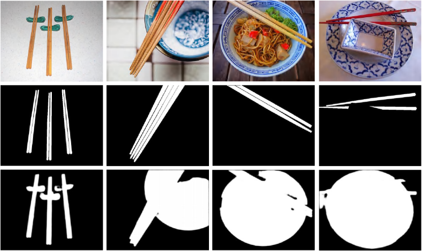
Figure 8: Failure cases of our method. From top to bottom are images, ground truths and our predictions. The chopsticks are the co-salient objects of this group.

4.5 Failure Case

For some extremely challenging scenarios, our method cannot successfully segment the co-salient objects. Take the images in Fig. 8 as an example, the chopsticks are the co-salient objects of this group. However, the salient object bowls appear in most of the images. Meanwhile, chopsticks are smaller objects compared with bowls. and the bowls are more salient than the chopsticks. In this case, it is difficult to eliminate noise from the bowls and extract a pure co-representation, so that the predictions are inaccurate.

4.6 Extention to Co-Segmentation

To validate the universal effectiveness of our CoRP, we extend our method to the field of image co-segmentation. In fact, image co-segmentation is similar to Co-SOD. Both of the two tasks aim at segmenting the common objects among a group of relevant images. The difference is that image co-segmentation does not need the co-objects to be salient. Our method, which aims at solving complex scenarios in Co-SOD, is also very effective in co-segmentation.

We also qualitatively compare our CoRP with popular co-segmentation methods on the three co-segmentation benchmark datasets, including MSRC dataset [65], iCoseg dataset [66], and Internet dataset [67]. We report the performances of the co-segmentation models using two wildly used metrics: Precision and Jaccard.

The Tab. VIII shows that on Internet dataset, our outperform the other methods across all categories and all metrics. Our improvement in terms of Jaccard is very obvious. Compared with the second-best method, our method brings 17.3% improvement on the overall dataset. In terms of Precision, our method also brings 0.6% improvement. In Tab. IX, we compare our method with others in terms of Jaccard. Once again, we outperform other methods in all categories. On the overall iCoseg dataset, our method brings 2.5% improvement compared with the second-best method. Further, the Tab. X reveals that on MSRC dataset, our method respectively bring 1.7% and 3.7% performance improvement in term of Precision and Jaccard. In Fig. 9, we present two groups (car and bird) of our predictions. It shows that our method segments the target objects with high accuracy.

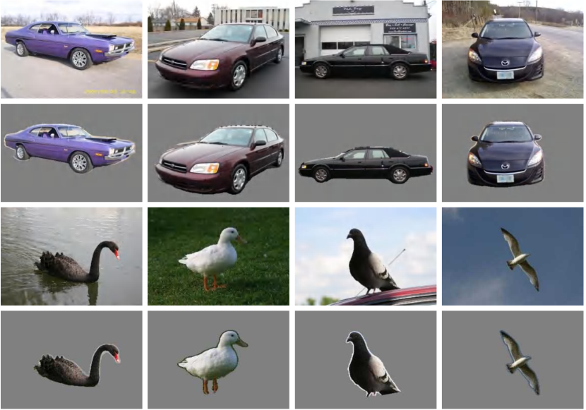
Figure 9: Our qualitative results on the co-segmentation datasets.

5 Conclusions

In this paper, we observe that current Co-SOD methods have not paid due attention to the noise in co-representation which is crucial for Co-SOD task, so that their performance suffer from the complex foreground objects’ interference. To overcome this shortcoming, we focus on eliminating the distracting information in the co-representation and propose an effective method (CoRP). Our CoRP works iteratively with two collaborative strategies (PCS and RPP), which aim at suppressing the noise in the co-representation to acquire more accurate prediction. In a nutshell, PCS is designed for searching pure co-representation from the sparse locations belonging to co-salient objects with the help of co-representation proxy provided by RPP, then our PCS feedbacks newly predicted co-saliency maps to RPP. Again, RPP uses the newly predictions to calculate a co-representation proxy with less distracting information in turn. In this way, the co-representation and prediction are utilized to improve each other in an iterative process. Substantial visualization results and experimental analysis demonstrate our contributions. Our CoRP achieves SOTA results on three challenging datasets.

Acknowledgement.  This research was supported by the NSFC (62176130) and the Fundamental Research Funds for the Central Universities (Nankai University, NO. 63223050).

Zi-Yue Zhu is currently a master student from the College of Computer Science at Nankai University, under the supervision of Prof. Ming-Ming Cheng. His research interests include deep learning and computer vision.

Zhao Zhang is currently a researcher at SenseTime Group LTD. He received a Master’s degree at Nankai University under the supervision of Prof. Ming-Ming Cheng, and a Bachelor’s degree at Yangzhou University. His research interests mainly focus on image processing, computer vision, and deep learning.

Zheng Lin is currently a Ph.D. candidate with College of Computer Science, Nankai University, under the supervision of Prof. Ming-Ming Cheng. His research interests include deep learning, computer graphics, and computer vision.

Xing Sun is currently a Principal researcher in Tencent YoutuLab. Before that, he received his Ph.D. degree from The University of Hong Kong in 2016. His research interests include image processing, machine learning, and computer vision.

Ming-Ming Cheng received his PhD degree from Tsinghua University in 2012. Then he did 2 years research fellow, with Prof. Philip Torr in Oxford. He is now a professor at Nankai University, leading the Media Computing Lab. His research interests includes computer graphics, computer vision, and image processing. He received research awards including ACM China Rising Star Award, IBM Global SUR Award, CCF-Intel Young Faculty Researcher Program, etc.

References

- [1] R. Cong, J. Lei, H. Fu, M.-M. Cheng, W. Lin, and Q. Huang, “Review of visual saliency detection with comprehensive information,” IEEE Trans. Circuit Syst. Video Technol., vol. 29, no. 10, pp. 2941–2959, 2018.
- [2] K. R. Jerripothula, J. Cai, and J. Yuan, “Cats: Co-saliency activated tracklet selection for video co-localization,” in Eur. Conf. Comput. Vis., 2016, pp. 187–202.
- [3] A. Joulin, K. Tang, and L. Fei-Fei, “Efficient image and video co-localization with frank-wolfe algorithm,” in Eur. Conf. Comput. Vis., 2014, pp. 253–268.
- [4] Y. Zeng, Y. Zhuge, H. Lu, and L. Zhang, “Joint learning of saliency detection and weakly supervised semantic segmentation,” in Int. Conf. Comput. Vis., 2019, pp. 7223–7233.
- [5] X. Wang, X. Liang, B. Yang, and F. W. Li, “No-reference synthetic image quality assessment with convolutional neural network and local image saliency,” Computational Visual Media, vol. 5, no. 2, pp. 193–208, 2019.
- [6] L. Zhang, J. Zhang, Z. Lin, H. Lu, and Y. He, “Capsal: Leveraging captioning to boost semantics for salient object detection,” in IEEE Conf. Comput. Vis. Pattern Recog., 2019, pp. 6024–6033.
- [7] C.-C. Tsai, W. Li, K.-J. Hsu, X. Qian, and Y.-Y. Lin, “Image co-saliency detection and co-segmentation via progressive joint optimization,” IEEE Trans. Image Process., vol. 28, no. 1, pp. 56–71, 2018.
- [8] L. Wei, S. Zhao, O. E. F. Bourahla, X. Li, F. Wu, and Y. Zhuang, “Deep group-wise fully convolutional network for co-saliency detection with graph propagation,” IEEE Trans. Image Process., vol. 28, no. 10, pp. 5052–5063, 2019.
- [9] Z.-J. Zha, C. Wang, D. Liu, H. Xie, and Y. Zhang, “Robust deep co-saliency detection with group semantic and pyramid attention,” IEEE Trans. Neural Netw. Learn. Syst., vol. 31, no. 7, pp. 2398–2408, 2020.
- [10] K. Zhang, T. Li, S. Shen, B. Liu, J. Chen, and Q. Liu, “Adaptive graph convolutional network with attention graph clustering for co-saliency detection,” in IEEE Conf. Comput. Vis. Pattern Recog., 2020, pp. 9050–9059.
- [11] K. Zhang, T. Li, B. Liu, and Q. Liu, “Co-saliency detection via mask-guided fully convolutional networks with multi-scale label smoothing,” in IEEE Conf. Comput. Vis. Pattern Recog., 2019, pp. 3095–3104.
- [12] D.-P. Fan, T. Li, Z. Lin, G.-P. Ji, D. Zhang, M.-M. Cheng, H. Fu, and J. Shen, “Re-thinking co-salient object detection,” IEEE Trans. Pattern Anal. Mach. Intell., 2021.
- [13] Z. Zhang, W. Jin, J. Xu, and M.-M. Cheng, “Gradient-induced co-saliency detection,” in Eur. Conf. Comput. Vis. Springer, 2020, pp. 455–472.
- [14] Q. Fan, D.-P. Fan, H. Fu, C. K. Tang, L. Shao, and Y.-W. Tai, “Group collaborative learning for co-salient object detection,” IEEE Conf. Comput. Vis. Pattern Recog., 2021.
- [15] W.-D. Jin, J. Xu, M.-M. Cheng, Y. Zhang, and W. Guo, “Icnet: Intra-saliency correlation network for co-saliency detection,” Adv. Neural Inform. Process. Syst., vol. 33, 2020.
- [16] Q. Zhang, R. Cong, J. Hou, C. Li, and Y. Zhao, “CoADNet: Collaborative aggregation-and-distribution networks for co-salient object detection,” in Adv. Neural Inform. Process. Syst., 2020.
- [17] L. Van der Maaten and G. Hinton, “Visualizing data using t-sne.” Journal of machine learning research, vol. 9, no. 11, 2008.
- [18] D.-P. Fan, Z. Lin, G.-P. Ji, D. Zhang, H. Fu, and M.-M. Cheng, “Taking a deeper look at co-salient object detection,” in IEEE Conf. Comput. Vis. Pattern Recog., 2020, pp. 2919–2929.
- [19] D. Zhang, J. Han, C. Li, J. Wang, and X. Li, “Detection of co-salient objects by looking deep and wide,” Int. J. Comput. Vis., vol. 120, no. 2, pp. 215–232, 2016.
- [20] D. E. Jacobs, D. B. Goldman, and E. Shechtman, “Cosaliency: Where people look when comparing images,” in Proceedings of the 23nd annual ACM symposium on User interface software and technology, 2010, pp. 219–228.
- [21] H. Li and K. N. Ngan, “A co-saliency model of image pairs,” IEEE Trans. Image Process., vol. 20, no. 12, pp. 3365–3375, 2011.
- [22] H.-T. Chen, “Preattentive co-saliency detection,” in IEEE Int. Conf. Image Process. IEEE, 2010, pp. 1117–1120.
- [23] H. Fu, X. Cao, and Z. Tu, “Cluster-based co-saliency detection,” IEEE Trans. Image Process., vol. 22, no. 10, pp. 3766–3778, 2013.
- [24] J. Han, G. Cheng, Z. Li, and D. Zhang, “A unified metric learning-based framework for co-saliency detection,” IEEE Trans. Circuit Syst. Video Technol., vol. 28, no. 10, pp. 2473–2483, 2017.
- [25] Y. Li, K. Fu, Z. Liu, and J. Yang, “Efficient saliency-model-guided visual co-saliency detection,” IEEE Sign. Process. Letters, vol. 22, no. 5, pp. 588–592, 2014.
- [26] X. Cao, Z. Tao, B. Zhang, H. Fu, and W. Feng, “Self-adaptively weighted co-saliency detection via rank constraint,” IEEE Trans. Image Process., vol. 23, no. 9, pp. 4175–4186, 2014.
- [27] K.-Y. Chang, T.-L. Liu, and S.-H. Lai, “From co-saliency to co-segmentation: An efficient and fully unsupervised energy minimization model,” in IEEE Conf. Comput. Vis. Pattern Recog. IEEE, 2011, pp. 2129–2136.
- [28] K.-J. Hsu, C.-C. Tsai, Y.-Y. Lin, X. Qian, and Y.-Y. Chuang, “Unsupervised cnn-based co-saliency detection with graphical optimization,” in Eur. Conf. Comput. Vis., 2018, pp. 485–501.
- [29] B. Li, Z. Sun, L. Tang, Y. Sun, and J. Shi, “Detecting robust co-saliency with recurrent co-attention neural network.” in IJCAI, 2019, pp. 818–825.
- [30] A. Borji, M.-M. Cheng, Q. Hou, H. Jiang, and J. Li, “Salient object detection: A survey,” Computational Visual Media, vol. 5, no. 2, pp. 117–150, 2019.
- [31] L. Itti, C. Koch, and E. Niebur, “A model of saliency-based visual attention for rapid scene analysis,” IEEE Trans. Pattern Anal. Mach. Intell., vol. 20, no. 11, pp. 1254–1259, 1998.
- [32] M.-M. Cheng, N. J. Mitra, X. Huang, P. H. Torr, and S.-M. Hu, “Global contrast based salient region detection,” IEEE Trans. Pattern Anal. Mach. Intell., vol. 37, no. 3, pp. 569–582, 2015.
- [33] J. Wang, H. Jiang, Z. Yuan, M.-M. Cheng, X. Hu, and N. Zheng, “Salient object detection: A discriminative regional feature integration approach,” Int. J. Comput. Vis., vol. 123, no. 2, pp. 215–268, 2017.
- [34] X. Li, H. Lu, L. Zhang, X. Ruan, and M.-H. Yang, “Saliency detection via dense and sparse reconstruction,” in Int. Conf. Comput. Vis., 2013, pp. 2976–2983.
- [35] F. Perazzi, P. Krähenbühl, Y. Pritch, and A. Hornung, “Saliency filters: Contrast based filtering for salient region detection,” in IEEE Conf. Comput. Vis. Pattern Recog. IEEE, 2012, pp. 733–740.
- [36] J. Wei, S. Wang, and Q. Huang, “F3net: fusion, feedback and focus for salient object detection,” in Association for the Advancement of Artificial Intelligence, 2020, pp. 12 321–12 328.
- [37] Q. Hou, M.-M. Cheng, X. Hu, A. Borji, Z. Tu, and P. H. Torr, “Deeply supervised salient object detection with short connections,” in IEEE Conf. Comput. Vis. Pattern Recog., 2017, pp. 3203–3212.
- [38] J.-J. Liu, Q. Hou, Z.-A. Liu, and M.-M. Cheng, “Poolnet+: Exploring the potential of pooling for salient object detection,” IEEE Trans. Pattern Anal. Mach. Intell., 2022.
- [39] T.-Y. Lin, P. Dollár, R. Girshick, K. He, B. Hariharan, and S. Belongie, “Feature pyramid networks for object detection,” in IEEE Conf. Comput. Vis. Pattern Recog., 2017, pp. 2117–2125.
- [40] X. Zhang, T. Wang, J. Qi, H. Lu, and G. Wang, “Progressive attention guided recurrent network for salient object detection,” in IEEE Conf. Comput. Vis. Pattern Recog., 2018, pp. 714–722.
- [41] N. Liu, J. Han, and M.-H. Yang, “Picanet: Learning pixel-wise contextual attention for saliency detection,” in IEEE Conf. Comput. Vis. Pattern Recog., 2018, pp. 3089–3098.
- [42] K. Simonyan and A. Zisserman, “Very deep convolutional networks for large-scale image recognition,” in Int. Conf. Learn. Represent., 2015.
- [43] A. Borji, M.-M. Cheng, H. Jiang, and J. Li, “Salient object detection: A benchmark,” IEEE Trans. Image Process., vol. 24, no. 12, pp. 5706–5722, 2015.
- [44] D.-P. Fan, M.-M. Cheng, Y. Liu, T. Li, and A. Borji, “Structure-measure: A new way to evaluate foreground maps,” in Int. Conf. Comput. Vis., 2017, pp. 4548–4557.
- [45] D.-P. Fan, C. Gong, Y. Cao, B. Ren, M.-M. Cheng, and A. Borji, “Enhanced-alignment measure for binary foreground map evaluation,” in IJCAI, 7 2018, pp. 698–704.
- [46] T. Liu, Z. Yuan, J. Sun, J. Wang, N. Zheng, X. Tang, and H.-Y. Shum, “Learning to detect a salient object,” IEEE Trans. Pattern Anal. Mach. Intell., vol. 33, no. 2, pp. 353–367, 2010.
- [47] K. He, X. Zhang, S. Ren, and J. Sun, “Deep residual learning for image recognition,” in IEEE Conf. Comput. Vis. Pattern Recog., 2016, pp. 770–778.
- [48] W. Wang, E. Xie, X. Li, D.-P. Fan, K. Song, D. Liang, T. Lu, P. Luo, and L. Shao, “Pyramid vision transformer: A versatile backbone for dense prediction without convolutions,” in Int. Conf. Comput. Vis., 2021, pp. 568–578.
- [49] Z. Guo, X. Zhang, H. Mu, W. Heng, Z. Liu, Y. Wei, and J. Sun, “Single path one-shot neural architecture search with uniform sampling,” 2020.
- [50] X. Zhao, Y. Pang, L. Zhang, H. Lu, and L. Zhang, “Suppress and balance: A simple gated network for salient object detection,” in Eur. Conf. Comput. Vis., 2020, pp. 35–51.
- [51] Z. Chen, Q. Xu, R. Cong, and Q. Huang, “Global context-aware progressive aggregation network for salient object detection,” in Association for the Advancement of Artificial Intelligence, 2020, pp. 10 599–10 606. [Online]. Available: https://aaai.org/ojs/index.php/AAAI/article/view/6633
- [52] K. Zhang, M. Dong, B. Liu, X.-T. Yuan, and Q. Liu, “Deepacg: Co-saliency detection via semantic-aware contrast gromov-wasserstein distance,” in IEEE Conf. Comput. Vis. Pattern Recog., 2021, pp. 13 703–13 712.
- [53] N. Zhang, J. Han, N. Liu, and L. Shao, “Summarize and search: Learning consensus-aware dynamic convolution for co-saliency detection,” in Int. Conf. Comput. Vis., 2021, pp. 4167–4176.
- [54] L. Wang, H. Lu, Y. Wang, M. Feng, D. Wang, B. Yin, and X. Ruan, “Learning to detect salient objects with image-level supervision,” in IEEE Conf. Comput. Vis. Pattern Recog., 2017, pp. 136–145.
- [55] T.-Y. Lin, M. Maire, S. Belongie, J. Hays, P. Perona, D. Ramanan, P. Dollár, and C. L. Zitnick, “Microsoft coco: Common objects in context,” in Eur. Conf. Comput. Vis., 2014, pp. 740–755.
- [56] A. Paszke, S. Gross, F. Massa, A. Lerer, J. Bradbury, G. Chanan, T. Killeen, Z. Lin, N. Gimelshein, L. Antiga et al., “PyTorch: An imperative style, high-performance deep learning library,” in Adv. Neural Inform. Process. Syst., 2019, pp. 8024–8035.
- [57] S.-M. Hu, D. Liang, G.-Y. Yang, G.-W. Yang, and W.-Y. Zhou, “Jittor: a novel deep learning framework with meta-operators and unified graph execution,” Science China Information Sciences, vol. 63, no. 222103, pp. 1–21, 2020.
- [58] H. Lin, X. Qi, and J. Jia, “Agss-vos: Attention guided single-shot video object segmentation,” in Int. Conf. Comput. Vis., 2019, pp. 3949–3957.
- [59] K. R. Jerripothula, J. Cai, and J. Yuan, “Image co-segmentation via saliency co-fusion,” IEEE Trans. Multimedia, vol. 18, no. 9, pp. 1896–1909, 2016.
- [60] W. Li, O. H. Jafari, and C. Rother, “Deep object co-segmentation,” in Asia Conf. Comput. Vis. Springer, 2018, pp. 638–653.
- [61] Y.-C. Chen, Y.-Y. Lin, M.-H. Yang, and J.-B. Huang, “Show, match and segment: Joint weakly supervised learning of semantic matching and object co-segmentation,” IEEE Trans. Pattern Anal. Mach. Intell., vol. 43, no. 10, pp. 3632–3647, 2020.
- [62] K. Zhang, J. Chen, B. Liu, and Q. Liu, “Deep object co-segmentation via spatial-semantic network modulation,” in Association for the Advancement of Artificial Intelligence, vol. 34, no. 07, 2020, pp. 12 813–12 820.
- [63] H. Chen, Y. Huang, and H. Nakayama, “Semantic aware attention based deep object co-segmentation,” in Asia Conf. Comput. Vis. Springer, 2018, pp. 435–450.
- [64] P. Mukherjee, B. Lall, and S. Lattupally, “Object cosegmentation using deep siamese network,” arXiv preprint arXiv:1803.02555, 2018.
- [65] J. Shotton, J. Winn, C. Rother, and A. Criminisi, “Textonboost: Joint appearance, shape and context modeling for multi-class object recognition and segmentation,” in Eur. Conf. Comput. Vis. Springer, 2006, pp. 1–15.
- [66] D. Batra, A. Kowdle, D. Parikh, J. Luo, and T. Chen, “icoseg: Interactive co-segmentation with intelligent scribble guidance,” in IEEE Conf. Comput. Vis. Pattern Recog. IEEE, 2010, pp. 3169–3176.
- [67] M. Rubinstein, A. Joulin, J. Kopf, and C. Liu, “Unsupervised joint object discovery and segmentation in internet images,” in IEEE Conf. Comput. Vis. Pattern Recog., 2013, pp. 1939–1946.