Like-charge attraction in one- and two-dimensional Coulomb systems

Abstract

[Summary]The bare Coulomb interaction between two like-charges is repulsive. When these charges are immersed in an electrolyte, the thermal fluctuations of the ions turn the bare Coulomb interaction into an effective interaction between the two charges. An interesting question arises: is it possible that the effective interaction becomes attractive for like-charges? We will show how this like-charge attraction phenomenon is indeed predicted in some one- and two-dimensional models of Coulomb systems. Exact analytical results can be obtained for these Coulomb systems models due to some connections that they have with integrable field theories. We will explain the techniques that allow obtaining exact results for the correlation functions between like-charge particles and how, under certain circumstances, the natural repulsion interaction shifts to being attractive. Although the technical details differ for 1d or 2d systems, the physical cause of this phenomenon is rooted in a three-body interaction between the two like-charges and an ion of the electrolyte with an opposite charge.

1 Introduction

Like-charge attraction is the intriguing phenomenon when two particles with charges of the same sign that are immersed in an electrolyte turn out to have an effective interaction that is attractive instead of the natural expected repulsion. The effective interaction accounts for all the collective effects of the particles and the surrounding ions of the electrolyte that are subject to thermal fluctuations. The like-charge attraction phenomenon has been evidenced in several experiments ^{1, 2} and numerical simulations ^{3, 4}. For some time a satisfactory explanation of this phenomenon was lacking. It was shown that it is impossible to have like-charge attraction in the low coulombic coupling regime, where the effective interactions can be computed using Poisson-Boltzmann theory and are always repulsive ^{5, 6, 7}. A plausible explanation to the experimental results from ² was given in ⁸ where a nonequilibrium hydrodynamic interaction could explain the like-charge attraction. Nevertheless the question of whether the like-charge attraction could be a consequence of only the electrostatic collective interactions remained open for some time. Advances in understanding the strongly Coulomb coupled regime ^{9, 10, 11, 12} shed some light on that question. A systematic high coupling expansion ¹³ revealed that in the strongly coupled regime like-charges can have an attractive interaction in some particular set of the parameters (coupling and distance between the particles) ¹⁴.

In parallel, there have been many advances in the theory of exactly solvable models of Coulomb systems in one dimension ^{15, 16, 17, 18} and two dimensions ^{19, 20, 21, 22, 23}. These are simplified models of point-charged particles living in $d=1$ or $d=2$ dimensions and interacting with the Coulomb potential corresponding to that dimension, namely, for two unit charges separated by a distance $r$,

$$v_{d}(r)=\begin{cases}-r&\text{for }d=1\\ -\ln r&\text{for }d=2\end{cases}.$$ (1)

These models provide a testing ground to understand several properties of classical charged systems. They also exhibit interesting connections with integrable quantum field theories. In this article, we present how the like-charge attraction phenomenon is predicted in several solvable models in one and two dimensions. In the section 2, we review results regarding like-charge attraction in 1d models. In section 3, we present some 2d models and extend some recent results to study the possibility of like-charge attraction in charge-asymmetric plasmas. Finally, we conclude with an overview of the like-charge attraction in the context of solvable models.

2 One-dimensional models

Consider a system of two equal charges $Q$ located in a line ($x$-axis) at $x=0$ and $x=L$ and screened by $N$ counterions with charge $e=-2Q/N$. The system is globally neutral. The charges $Q$ are at fixed positions, while the counterions can move between the two charges $Q$ and are at thermal equilibrium at a temperature $T$. As usual we define $\beta=1/(k_{B}T)$ with $k_{B}$ the Boltzmann constant. In one dimension, the potential energy between two particles of charges $q$ and $q^{\prime}$ located at $x$ and $x^{\prime}$ is

$$u_{1}(x,x^{\prime})=-qq^{\prime}|x-x^{\prime}|\,.$$ (2)

In one dimension, the charges $q$ have dimensions of $(\text{energy/length})^{1/2}=\text{force}^{1/2}$. Therefore one can define a characteristic length comparing the thermal energy with the electrostatic energy

$$l_{B}^{1d}=k_{B}T/e^{2}\,.$$ (3)

This is the one-dimensional equivalent of the Bjerrum length $l_{B}^{3d}$. Notice however the difference with the 3d situation where $l_{B}^{3d}=e_{3d}^{2}/(k_{B}T)$ for $e_{3d}$ the elementary 3d charge. This difference is due to the change in the Coulomb potential from $1/r$ in 3d to $-r$ in 1d. The 1d-charges have dimensions of 3d-charges/distance². The total potential energy $U$ of the system is given by

$$\beta U=-\sum_{1\leq i<j\leq N}\frac{|x_{i}-x_{j}|}{l_{B}^{1d}}+\left(\frac{N}{2}\right)^{2}\frac{L}{l_{B}^{1d}}\,.$$ (4)

At this point is useful to recall some properties of 1d electrostatics. The electric field at $x^{\prime}$ created by a single charge $q$ located at $x$ is constant and equal to $q$ for $x^{\prime}>x$ (right side of $q$) and equal to $-q$ for $x^{\prime}<x$ (left side). Therefore, the counterions feel a constant force so long they do not interchange positions with their neighbors. To obtain the force on a given counterion one simply has to sum all charges at its right and subtract the charges at its left. This greatly simplifies the analysis of the system to the point that by ordering the particle positions one can rewrite the potential energy (4) as a sum of differences of consecutive positions of the particles ($x_{k}-x_{k+1}$) as shown in ²⁴. With this one recognizes that the partition function of the system is an $N$-fold convolution product that can be explicitly computed using the Laplace transform which is equivalent to work in the isobaric ensemble ²⁴. From there the effective force between the two charges $Q$ is obtained as the derivative of the canonical partition function with respect to $L$. From those exact results, the possibility of like-charge attraction appears when $N=2p+1$ is an odd integer and for large distances $L$.

Beyond those exact results, it is instructive to recall here a simple argument ²⁴ which explains the like-charge attraction. Consider first the even case $N=2p$ and that the charges $Q$ are separated by a distance $L\gg l_{B}^{1d}$. The system will decouple into two parts. The charge $Q$ located at $x=0$ will be screened by a layer of $p=N/2$ counterions and the charge $Q$ located at $x=L$ will have its screening layer composed of the rest of the $p$ counterions. These two entities are neutral and they weakly interact with a repulsive force. In that situation, no like-charge attraction is observed. In the odd case, $N=2p+1$, frustration appears in this scenario. The counterions will try to screen each charge $Q$, but since $N$ is not divisible by two, a misfit ion remains between two layers of $p$ counterions around each charge $Q$. These two entities are not neutral now, they have a charge $Q+ep=-e/2$. This situation is illustrated in figure 1. The misfit counterion between the two feels a zero electric field because the electric field created by each entity cancels each other. This misfit counterion roams between the two charged entities. When it is close, say to the left entity, the charge of the entity plus the misfit ion is $+e/2$ which will create an effective attractive force to the right entity that has charge $-e/2$. The effective attractive force is

$$F\to-(e/2)^{2}\,\qquad\text{when }L\gg l_{B}^{1d}\,.$$ (5)

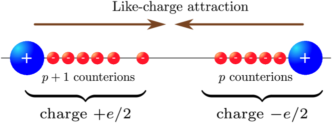
Figure 1: Illustration of the like-charge attraction in 1d systems due to an imbalance of charge when an odd number $N=2p+1$ of counterions is present.

Equation (5) gives the leading term of the force for large distances $L$. The next-to-leading term can also be obtained by a simple argument. The misfit ion has an available distance to move between the two screening layers equal to $L-2l_{S}$ where $l_{S}$ is the screening layer size around one of the charges $Q$. This layer size can be evaluated as the average position of the $p$-th counterion of the left side. With the Laplace transform technique, this has been computed exactly ²⁴

$$l_{S}=l_{B}^{1d}\frac{N-1}{N+1}.$$ (6)

The misfit ion is not subjected to any force, therefore its contribution to the effective force can be computed as the one of an ideal gas with one particle in a “volume" (distance in 1d) $L-2l_{S}$. It is $k_{B}T/(L-2l_{S})$. So, the effective force at large $L$ behaves as

$$F\to-(e/2)^{2}\ +\frac{k_{B}T}{L-2l_{S}}+o(1/L),\qquad\text{when }L\gg l_{B}^{1d}\,.$$ (7)

From this expression, one can evaluate the distance $L^{*}$ at which the force changes from repulsive ($L<L^{*}$) to attractive ($L>L*$)

$$L^{*}\simeq 4l_{B}^{1d}+2l_{S}=\left(4+2\frac{N-1}{N+1}\right)l_{B}^{1d}\,.$$ (8)

As an example, figure 2 shows a plot of the force as a function of the distance $L$ for the cases $N=10$ and $N=11$. For $N=10$ the force is always repulsive, while in the odd case $N=11$ the force is repulsive at short distance, then attractive for large distances $L$ beyond $L^{*}\simeq 5.67l_{B}^{1d}$.

Figure 2: The effective force between the charges $Q$ for the cases when the number of counterions is even $N=10$ and odd $N=11$. This latter case presents the like-charge attraction phenomenon.

Several extensions of this 1d model have been considered, including the case when the counterions can be also in the regions $x<0$ and $x>L$ ²⁵ and when there are dielectric inhomogeneities in those different regions ²⁶. When the dielectric constant outside (regions $x<0$ and $x>L$) is larger than inside (region $0<x<L$) it is possible to have like charge attraction even when $N$ is even due to the effect of image charges.

In the odd case $N=2p+1$, the misfit ion plays a central role in the like-charge attraction phenomenon. In ²⁷ the dynamics of the relaxation to a thermal equilibrium of the screening layers have been studied. Imposing an overdamped Langevin dynamics to the counterions, it is observed that the misfit ion rules the relaxation time $\tau$ of the system. For large distances $L\gg l_{B}^{1d}$ and an odd number of particles, $\tau\propto L^{2}/D$, where $D$ is the diffusion coefficient. On the other hand, for an even number of counterions, $L$ does not play any role. Instead, the relaxation time is $\tau=4(l_{B}^{1d})^{2}/D$. Notice also that the temperature dependency of $\tau$ changes drastically. Recalling that $D\propto T$, we notice that in the odd case, $\tau\propto 1/T$, whereas for $N$ even, $\tau\propto T$. Thus, when $N$ is odd, the higher the temperature, the faster the system equilibrates. This is because the misfit ion can roam faster between both layers. On the other hand, if $N$ is even, the relaxation time is reduced if the temperature is low. In this case, the physical mechanism ruling the relaxation is the formation of the layers, which will be faster if the temperature is lower and the electrostatic coupling is larger.

3 Two-dimensional models

3.1 Connection with integrable quantum field theories

We move on in this section to study two-dimensional systems. Let us consider a plasma living in a 2d plane composed of two types of particles of charges $q_{+}>0$ and $-q_{-}<0$. The potential energy between two charges $q$ and $q^{\prime}$ separated by a distance $r$ on the 2d plane is $-qq^{\prime}\ln r$. In 2d, the dimensions of a charge $q$ is $\text{energy}^{1/2}$. Comparing the electrostatic energy to the thermal energy, we obtain an important adimensional coupling constant of the system: $\beta q_{+}q_{-}$. We consider here a system of point particles. Because of the attractive interaction between positive and negative charges, the system of point particles is stable against the collapse of oppositely charged particles only if $\beta q_{+}q_{-}<2$. We will restrict the following analysis to that stability regime. The potential energy of the system composed by $N_{+}$ positive charge located at positions $\{{\mathbf{r}}_{j}^{+}\}$ and $N_{-}$ negative charges located at $\{{\mathbf{r}}_{k}^{+}\}$ is

$$U_{N_{+},N_{-}} =-q_{+}^{2}\sum_{1\leq k<j\leq N_{+}}\ln|{\mathbf{r}}_{j}^{+}-{\mathbf{r}}_{k}^{+}|-q_{-}^{2}\sum_{1\leq k<j\leq N_{+}}\ln|{\mathbf{r}}_{j}^{-}-{\mathbf{r}}_{k}^{-}|+q_{+}q_{-}\sum_{j=1}^{N_{+}}\sum_{k=1}^{N_{-}}\ln|{\mathbf{r}}_{k}^{-}-{\mathbf{r}}_{j}^{+}|\,.$$ (9)

The grand canonical partition function of the system with fugacities $z_{+}$ and $z_{-}$ for the positive and negative particles respectively is

$$\Xi=\sum_{N_{+}=0}^{\infty}\sum_{N_{-}=0}^{\infty}\frac{z_{+}^{N_{+}}}{N_{+}!}\frac{z_{-}^{N_{-}}}{N_{-}!}e^{-\beta U_{N_{+},N_{-}}}\prod_{j=1}^{N_{+}}d{\mathbf{r}}_{j}^{+}\prod_{k=1}^{N_{-}}d{\mathbf{r}}_{k}^{-}\,.$$ (10)

By using the Hubbard-Stratonovich transformation ^{28, 29}, the grand partition function (10) can be transformed into the generating functional of a quantum field theory

$$\Xi=\frac{Z(z_{+},z_{-})}{Z(0,0)},$$ (11)

where

$$Z(z_{+},z_{-})=\int\mathcal{D}\phi\,e^{-S(z_{+},z_{-})},$$ (12)

with

$$S(z_{+},z_{-})=-\int\left[\frac{\beta}{4\pi}\phi({\mathbf{r}})\Delta\phi({\mathbf{r}})+z_{+}e^{i\beta q_{+}\phi({\mathbf{r}})}+z_{-}e^{-i\beta q_{-}\phi({\mathbf{r}})}\right]\,d{\mathbf{r}}\,.$$ (13)

Two special cases are worth mentioning. When $q_{+}=q_{-}$, the equivalent quantum field theory is the sine-Gordon model. For $q_{+}=2q_{-}$ or $q_{-}=2q_{+}$, the quantum field theory is the Dodd-Bullough model. In two dimensions, these two field theories are integrable and many of their properties (spectrum, S-matrix, expectations of exponential field, form factors, …) have been computed exactly ^{30, 31, 32, 33, 34, 35, 36, 37}. Using these results, the exact equilibrium thermodynamic properties of the 2d plasma have been obtained for the charge-symmetric situation ²³ $q_{+}=q_{-}$ and the charge-asymmetric situation ³⁸ with $q_{+}=2q_{-}$ or $q_{-}=2q_{+}$. Beyond those two particular cases, the equivalent field theory has not been solved exactly.

Consider now two external charges $Q_{1}$ and $Q_{2}$ immersed in the plasma at $0$ and ${\mathbf{r}}$. For the following analysis to remain valid it is necessary to be in the stability regime, not only for the plasma charges ($\beta q_{+}q_{-}<2$) but also for the guest charges against the collapse with a plasma charge of opposite sign

$$-2/q_{+}<\beta Q_{k}<2/q_{-},\qquad\text{for }k\in\{1,2\}.$$ (14)

Averaging over the thermal fluctuations of the plasma ions, the effective interaction $G_{Q_{1}Q_{2}}(r)$ between these two charges is defined by

$$e^{-\beta G_{Q_{1}Q_{2}}(r)}=\frac{\Xi[Q_{1},0;Q_{2},{\mathbf{r}}]/\Xi}{(\Xi[Q_{1}]/\Xi)\,(\Xi[Q_{2}]/\Xi)},$$ (15)

where $\Xi[Q_{1},0;Q_{2},{\mathbf{r}}]$ is the partition function of the plasma in the presence of the charges $Q_{1}$ and $Q_{2}$ separated by a distance $r$, while $\Xi[Q_{1}]$ and $\Xi[Q_{2}]$ are the partition functions of the plasma with only one guest charge $Q_{1}$ or $Q_{2}$ immersed in it. In the formalism of the equivalent quantum field theory, the effective interaction $G_{Q_{1}Q_{2}}(r)$ can be cast as

$$e^{-\beta G_{Q_{1}Q_{2}}(r)}=\frac{\left<e^{i\beta Q_{1}\phi(0)}e^{i\beta Q_{2}\phi({\mathbf{r}})}\right>}{\left<e^{i\beta Q_{1}\phi(0)}\right>\left<e^{i\beta Q_{2}\phi({\mathbf{r}})}\right>},$$ (16)

where the average $\left<\cdots\right>$ is taken over the fluctuations of the field $\phi$ with the weight defined in (12) and (13).

For the particular cases of the charge-symmetric plasma and charge-asymmetric plasma with $q_{+}/q_{+}$ equal to $2$ or $1/2$, using the equivalent sine-Gordon or Dodd-Bullough theory, it is possible to obtain the asymptotic behavior of $G_{Q_{1}Q_{2}}(r)$ for $r\to 0$ or $r\to\infty$. For $r\to 0$ the technique is based on the operator product expansion ^{39, 40}, while for large distances an expansion in form factors is used ^{41, 42, 43, 44}. Interestingly, in the charge-asymmetric plasma with $q_{+}/q_{-}=2$ or $1/2$, the phenomenon of like-charge attraction appears at short distance ⁴⁰ and a related phenomenon of charge inversion is noticed at large distances ⁴⁴. In the following, we generalize the findings of like-charge attraction at short distance ⁴⁰ for arbitrary charge asymmetry ($q_{+}/q_{-}$ can take arbitrary values).

3.2 Dominant term in the effective interaction

Starting from the definition (15) of the effective interaction $G_{Q_{1}Q_{2}}$, we notice that the dependence on the distance $r$ between the charges is only on the term

$$\Xi[Q_{1},0;Q_{2},{\mathbf{r}}]=\sum_{N_{+}=0}^{\infty}\sum_{N_{+}=0}^{\infty}\frac{z_{+}^{N_{+}}}{N_{+}!}\frac{z_{-}^{N_{-}}}{N_{-}!}Z_{N_{+},N_{-}}[Q_{1},0;Q_{2},{\mathbf{r}}].$$ (17)

In (17) appears a sum of configurational integrals of the two fixed charges $Q_{1}$ and $Q_{2}$ in the presence of $N_{+}$ positive charges and $N_{-}$ positive charges

$$Z_{N_{+},N_{-}}[Q_{1},0;Q_{2},{\mathbf{r}}]=\int e^{-\beta{\cal U}_{N_{+},N_{-}}[Q_{1},0;Q_{2},{\mathbf{r}}]}\,\prod_{j=1}^{N^{+}}d{\mathbf{r}}_{j}^{+}\prod_{k=1}^{N^{-}}d{\mathbf{r}}_{k}^{-},$$ (18)

with

$${\cal U}_{N_{+},N_{-}}[Q_{1},0;Q_{2},{\mathbf{r}}]= -Q_{1}Q_{2}\ln|{\mathbf{r}}|$$ (19)

$$-Q_{1}q_{+}\sum_{j=1}^{N_{+}}\ln|{\mathbf{r}}_{j}^{+}|+Q_{1}q_{-}\sum_{k=1}^{N_{-}}\ln|{\mathbf{r}}_{k}^{-}|$$ (20)

$$-Q_{2}q_{+}\sum_{j=1}^{N_{+}}\ln|{\mathbf{r}}-{\mathbf{r}}_{j}^{+}|+Q_{2}q_{-}\sum_{k=1}^{N_{-}}\ln|{\mathbf{r}}-{\mathbf{r}}_{k}^{-}|$$ (21)

$$+U_{N_{+},N_{-}}\,.$$ (22)

The explicit dependence on $r=|{\mathbf{r}}|$ of $Z_{N_{+},N_{-}}[Q_{1},0;Q_{2},{\mathbf{r}}]$ can be obtained by simple dimensional analysis. Let $(r,\theta)$ be the polar coordinates of ${\mathbf{r}}$. Using complex coordinates, one can make a change of variables on the plasma charges positions to rescale them by $r$ and rotate them so that the charge $Q_{2}$ is formally located at $1$. Explicitly, $z_{j}^{+}=(r_{j}^{+}/r)e^{i(\theta_{j}^{+}-\theta)}$ and $z_{k}^{-}=(r_{k}^{-}/r)e^{i(\theta_{k}^{-}-\theta)}$. Then

$$Z_{N_{+},N_{-}}[Q_{1},0;Q_{2},{\mathbf{r}}]=r^{\beta Q_{1}Q_{2}+f(Q_{1}+Q_{2};N_{+},N_{-})}Z_{N_{+},N_{-}}[Q_{1},0;Q_{2},1],$$ (23)

with

$$f(Q,N_{+},N_{-})=N_{+}(2-\beta q_{+}^{2}/2)+N_{-}(2-\beta q_{-}^{2}/2)+\beta Q(q_{+}N_{+}-q_{-}N_{-})+\beta(q_{+}N_{+}-q_{-}N_{-})^{2}/2,$$ (24)

and

$$Z_{N_{+},N_{-}}[Q_{1},0;Q_{2},1]=\int \frac{\prod_{j=1}^{N_{+}}|z_{j}^{+}|^{\beta q_{+}Q_{1}}|1-z_{j}^{+}|^{\beta q_{+}Q_{2}}}{\prod_{k=1}^{N_{-}}|z_{k}^{-}|^{\beta q_{-}Q_{1}}|1-z_{k}^{-}|^{\beta q_{-}Q_{2}}}$$

$$\times\frac{\prod_{1\leq j<k\leq N_{+}}|z_{j}^{+}-z_{k}^{+}|^{\beta q_{+}^{2}}\prod_{1\leq j<k\leq N_{-}}|z_{j}^{-}-z_{k}^{-}|^{\beta q_{-}^{2}}}{\prod_{j=1}^{N_{+}}\prod_{k=1}^{N_{-}}|z_{j}^{+}-z_{k}^{-}|^{\beta q_{+}q_{-}}}\prod_{j=1}^{N_{+}}d^{2}z_{j}^{+}\prod_{k=1}^{N_{-}}d^{2}z_{k}^{-}\,.$$ (25)

From the previous expressions, we notice that $\exp(-\beta G_{Q_{1}Q_{2}}(r))$ is given by a sum of terms with power law dependency on the distance between the charges: $r^{\beta Q_{1}Q_{2}+f(Q_{1}+Q_{2},N_{+},N_{-})}$. Physically this is interpreted as the contributions to the effective potential when the charges $Q_{1}$ and $Q_{2}$ are successively screened by $N_{+}$ positive charges and $N_{-}$ negative charges of the plasma. In the context of the equivalent field theory, this is the product operator expansion used in ^{39, 40}. For small distances $r\to 0$, one can analyze the behavior of the effective potential by determining the dominant term in this expansion as follows.

For sufficiently small values of $\beta$, $|Q_{1}|$ and $|Q_{2}|$ we have $f(Q_{1},Q_{2},N_{+},N_{-})\geq f(Q_{1},Q_{2},0,0)=0$. Therefore the dominant term in (17) for $r\to 0$ is obtained when $N_{+}=0$ and $N_{-}=0$,

$$\Xi[Q_{1},0;Q_{2},{\mathbf{r}}]\sim e^{\beta Q_{1}Q_{2}},$$ (26)

and the effective interaction behaves like a bare Coulomb potential

$$G_{Q_{1}Q_{2}}(r)\sim-Q_{1}Q_{2}\ln r.$$ (27)

However as $\beta$, $|Q_{1}|$ and $|Q_{2}|$ increase, it is possible that $f(Q_{1},Q_{2},N_{+},N_{-})<0$ for some values of $N_{+}$ and $N_{-}$. This will induce a change in the short distance behavior of $G_{Q_{1}Q_{2}}(r)$ from the bare Coulomb potential to a different behavior. These changes were first predicted in⁴⁵ for the correlation functions of a homogenous plasma by an analysis in the canonical ensemble. Here we focus on the situation with the two guest charges $Q_{1}$ and $Q_{2}$ and derive those changes working in the grand canonical ensemble setting which simplifies the analysis.

To fix the ideas, consider $Q_{1}<0$ and $Q_{2}<0$. Let us find when a term $f(Q,N_{+}+1,N_{-})$ dominates over a term $f(Q,N_{+},N_{-})$ where $Q=Q_{1}+Q_{2}$. The dominant term will be the smaller one. Since

$$f(Q,N_{+},N_{-})-f(Q,N_{+}+1,N_{-})=2+\beta q_{+}(Q+q_{+}N_{+}-q_{-}N_{-})\,.$$ (28)

Then $f(Q,N_{+}+1,N_{-})$ dominates over $f(Q,N_{+},N_{-})$ when

$$\beta q_{+}Q<-2-\beta q_{+}(q_{+}N_{+}-q_{-}N_{-}).$$ (29)

Notice that this corresponds exactly to the stability threshold for a negative cluster of charge $Q+q_{+}N_{+}-q_{-}N_{-}$:

$$\beta(Q+q_{+}N_{+}-q_{-}N_{-})<-2/q_{+}.$$ (30)

However, since the charges $Q_{1}$ and $Q_{2}$ are not located in the same position $r\neq 0$ it is possible to be in a situation where (30) occurs but the individual charges are still in their stability regime (14) guaranteeing that $\Xi[Q_{1},0;Q_{2},{\mathbf{r}}]$ does not diverges. The physical interpretation is that a term with $r$-power law $\beta Q_{1}Q_{2}+f(Q,N_{+},N_{-})$ dominates as long as the cluster of negative charge $Q+q_{+}N_{+}-q_{-}N_{-}$ is bounded below by $-2/q_{+}$. As soon as it crosses this value, an additional ion $q_{+}$ comes into the picture to strengthen the cluster screening and the $r$-power law will change to $\beta Q_{1}Q_{2}+f(Q,N_{+}+1,N_{-})$. To complete the analysis we have to compare also with the term with $N_{+}-1$ positive charges and $N_{-}$ negative charges. This follows simply by changing $N_{+}$ by $N_{+}-1$ in the previous analysis, to conclude that the contribution from the cluster with charge $Q+q_{+}N_{+}-q_{-}N_{-}$ is dominant over other clusters with different values of $N_{+}$ whenever

$$-2-\beta q_{+}(q_{+}N_{+}-q_{-}N_{-})<\beta q_{+}Q<-2-\beta q_{+}(q_{+}(N_{+}-1)-q_{-}N_{-})<0.$$ (31)

When $\beta q_{+}Q$ becomes smaller than the lower bound, the term with an additional $q_{+}$ ion becomes dominant (cluster of charge $Q+q_{+}(N_{+}+1)-q_{-}N_{-}$). On the other hand when $\beta q_{+}Q$ was larger than the upper bound, the dominant term was for a cluster of charge $Q+q_{+}(N_{+}-1)-q_{-}N_{-}$.

Similarly, if we consider positive guest charges $Q_{1}>0$ and $Q_{2}>0$, the regime where a cluster of charge $Q+q_{-}N_{-}-q_{+}N_{+}$ is dominant is when

$$0<2+\beta q_{-}(q_{-}(N_{-}-1)-q_{+}N_{+})<\beta q_{-}Q<2+\beta q_{-}(q_{-}N_{-}-q_{+}N_{+}).$$ (32)

When $\beta q_{-}Q$ was below the lower bound, the dominant term was given by a cluster of charge $Q-q_{-}(N_{-}-1)+q_{+}N_{+}$, and when it surpasses the upper bound, the dominant term is given by a cluster with an additional negative ion (charge $Q-q_{-}(N_{-}+1)+q_{+}N_{+}$).

Continuing with the case of positive guest charges, let us suppose that the condition (32) is satisfied so the contribution from a cluster of charge $Q-q_{-}N_{-}+q_{+}N_{+}$ dominates over other clusters with a different number of negative ions $N_{-}^{\prime}\neq N_{-}$. How does the contribution of this cluster compare with the one from another cluster with a different number $N_{+}^{\prime}$ of positive ions? Let us compare it with a cluster with $N_{+}-1$ positive ions. We have

$$f(Q,N_{+},N_{-})-f(Q,N_{+}-1,N_{-})=2+\beta q_{+}(Q+q_{+}(N_{+}-1)-q_{-}N_{-})+2.$$ (33)

Since $Q$ satisfies (32), we have

$$f(Q,N_{+},N_{-})-f(Q,N_{+}-1,N_{-})>(2-\beta q_{+}q_{-})q_{+}/q_{-}+1>1>0,$$ (34)

where we used the stability condition $\beta q_{+}q_{-}<2$. Therefore the contribution from a cluster with $N_{+}-1$ positive will dominate. Repeating this recursively we deduce that the cluster that will dominate is the one without positive ions ($N_{+}=0$) and $N_{-}$ negative ions. In conclusion, to obtain the dominant behavior we need to consider only clusters with ions of opposite charge to the guest charges. For $Q_{1}>0$ and $Q_{2}>0$, this means that the successive changes in the dominant behavior of the effective interaction will be given by the contributions of clusters of charge $Q_{1}+Q_{2}-q_{-}N_{-}$ when

$$0<2+\beta q_{-}^{2}(N_{-}-1)<\beta q_{-}(Q_{1}+Q_{2})<2+\beta q_{-}^{2}N_{-}.$$ (35)

For negative guest charges, it is the cluster of charge $Q_{1}+Q_{2}+q_{+}N_{+}$ that dominates when

$$-2-\beta q_{+}^{2}N_{+}<\beta q_{+}(Q_{1}+Q_{2})<-2-\beta q_{+}^{2}(N_{+}-1)<0.$$ (36)

The effective interaction between $Q_{1}$ and $Q_{2}$ is given by

$$G_{Q_{1}Q_{2}}(r)\sim(Q_{1}Q_{2}+\beta^{-1}f(Q_{1}+Q_{2},N_{+},N_{-}))\ln r,$$ (37)

with $N_{+}=0$ and a given value of $N_{-}\geq 0$ when $Q_{1}+Q_{2}$ satisfies (35), or $N_{-}=0$ and a given value of $N_{+}\geq 0$ when (36) is satisfied. This is illustrated in figure 3.

Figure 3: Graphical illustration of the dominant term in the effective interaction depending on the sum $Q_{1}+Q_{2}$ of the guest charges.

3.3 Like-charge attraction

To analyze the possibility of like-charge attraction, one has to determine the sign of $\beta Q_{1}Q_{2}+f(Q_{1}+Q_{2},N_{+},N_{-})$ in the dominant behavior (37) of $G_{Q_{1}Q_{2}}(r)$ when $Q_{1}$ and $Q_{2}$ have the same sign. Without loss of generality let us consider the case $Q_{1}>0$ and $Q_{2}>0$. The opposite case follows by interchanging the roles of $q_{+}$ and $q_{-}$. The bare interaction $-Q_{1}Q_{2}\ln r$ is repulsive. Let us explore the regions after the first change of behavior of $G_{Q_{1}Q_{2}}$, when $N_{-}\geq 1$ negative ions and $N_{+}=0$ positive ions form a cluster with $Q_{1}$ and $Q_{2}$. Let us define

$$\tilde{Q}_{k}=\beta Q_{k}q_{-}/2,\quad\text{for }k\in\{1,2\},$$ (38)

and

$$\tilde{q}_{-}=\beta q_{-}^{2}/2.$$ (39)

Because of the stability condition $(\tilde{Q}_{1},\tilde{Q}_{2})\in[0,1)^{2}$ and $\tilde{q}_{-}\in[0,q_{-}/q_{+})$. With this notation, the condition (35) can be written as

$$1+(N_{-}-1)\tilde{q}_{-}<\tilde{Q}_{1}+\tilde{Q}_{2}<1+N_{-}\tilde{q}_{-}.$$ (40)

When this is satisfied, the effective interaction at short distances is given by

$$\beta G_{Q_{1}Q_{2}}(r)\sim(\beta Q_{1}Q_{2}+f(Q_{1},Q_{2},0,N_{-}))\ln r.$$ (41)

This interaction is repulsive as long as $\beta Q_{1}Q_{2}+f(Q_{1},Q_{2},0,N_{-})>0$ and it will become attractive as soon as that quantity becomes negative. This condition can be cast as

$$g(\tilde{Q}_{1},\tilde{Q}_{2})<g(0,1+\tilde{q}_{-}(N_{-}-1)/2),$$ (42)

where we defined

$$g(\tilde{Q}_{1},\tilde{Q}_{2})=(\tilde{Q}_{1}-N_{-}\tilde{q}_{-})(\tilde{Q}_{2}-N_{-}\tilde{q}_{-})\,.$$ (43)

The separatrix between the repulsive and attractive regions is defined by the hyperbolas

$$g(\tilde{Q}_{1},\tilde{Q}_{2})=g(0,1+\tilde{q}_{-}(N_{-}-1)/2),$$ (44)

which have asymptotes at $\tilde{Q}_{1}=N_{-}\tilde{q}_{-}$ and $\tilde{Q}_{2}=N_{-}\tilde{q}_{-}$ and they pass thru the points $(\tilde{Q}_{1},\tilde{Q}_{2})=(0,1+\tilde{q}_{-}(N_{-}-1)/2)$ and $(\tilde{Q}_{1},\tilde{Q}_{2})=(1+\tilde{q}_{-}(N_{-}-1)/2,0)$. To determine if like-charge attraction is possible, we need to find if the region defined by (40) and (42) has a non empty intersection with the stability region $[0,1)^{2}$.

For this we need to distinguish two cases if $\tilde{q}_{-}<1$ or $\tilde{q}_{-}>1$. The situation when $\tilde{q}_{-}<1$ is shown in figure 4. The stability domain $[0,1)^{2}$ is divided into several regions depending on the behavior of the effective potential. Below the diagonal $\tilde{Q}_{1}+\tilde{Q}_{2}=1$, the effective interaction behaves like the bare Coulomb potential. This is the lower triangle of the square domain $[0,1)^{2}$. The upper triangle is divided by diagonal bands defined in (40). In each of these bands, the effective interaction behaves as (41). For $\tilde{q}_{-}<1$, several bands occupy the upper triangle up to $N_{-}<1+1/\tilde{q}_{-}$. For each of these zones, there is pair of hyperbolas defined by (44) for the corresponding value of $N_{-}$. If $\tilde{q}_{-}<1/2$, the l.h.s of 44 is negative $g(0,1+\tilde{q}_{-}(N_{-}-1)/2)<0$, and the corresponding hyperbolas lie on the left upper and right lower quadrants. Therefore the zone defined by (42) never intersects the stability region, see figure 4.

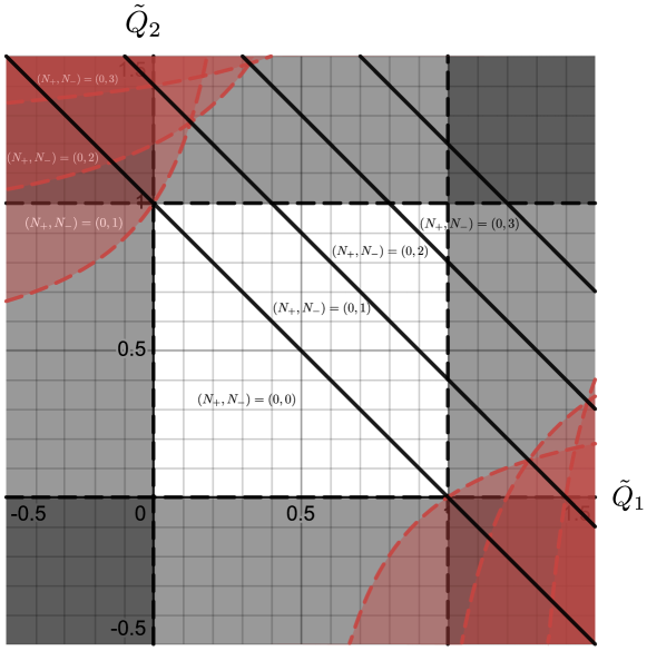
Figure 4: When $\tilde{q}_{-}<1$ (here $\tilde{q}_{-}=0.4$) the stability region in white does not intersect the region of possible like-charge attraction in red defined by (42). Since greyed zone is forbidden by the stability condition (14), the effective interaction remains always repulsive (white region). Notice that there are several changes in the effective interaction behavior depending on the bands that are shown in the upper triangle, each corresponding to a cluster of the guest charges with $N_{-}$ negative ions.

When $1/2<\tilde{q}_{-}<1$, it is possible that some hyperbolas switch sides to the upper right corner and the lower left corner. This happens when the l.h.s of 44 is positive $g(0,1+\tilde{q}_{-}(N_{-}-1)/2)>0$. This corresponds to $N_{-}>(2/\tilde{q}_{-})-1$. Nevertheless, the hyperbolas remain outside the stability region as long as $\tilde{q}_{-}<1$ as seen in figure 5. In conclusion, as illustrated in figures 4 and 5 there is never an intersection between the stability region and the region defined by (42). The regions where (42) is satisfied lie always in the forbidden zone outside the stability domain. In conclusion, the effective potential remains always repulsive when $\tilde{q}_{-}<1$.

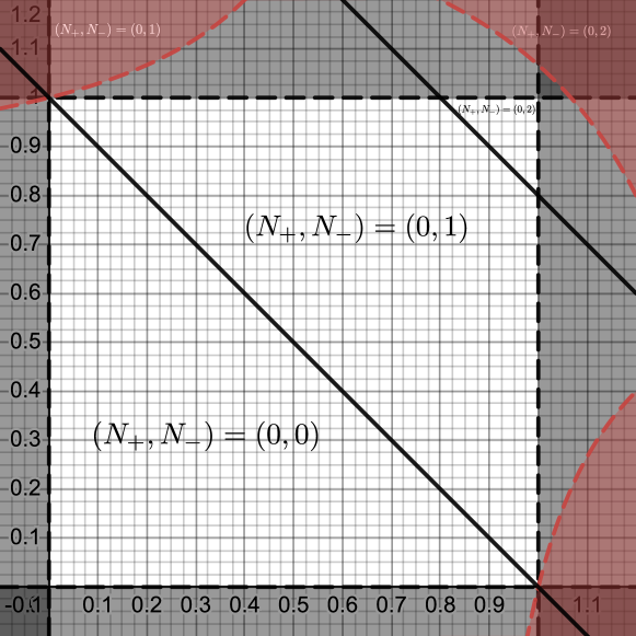
Figure 5: When $1/2<\tilde{q}_{-}<1$ (here $\tilde{q}_{-}=0.8$) one pair of hyperbolas (44) have switch sides. Nevertheless, the stability region in white does not intersect the region of possible like-charge attraction in red defined by (42). Since the greyed zone is forbidden by the stability condition (14), the effective interaction remains always repulsive (white region).

For $\tilde{q}_{-}\to 1^{-}$, the distance of the hyperbola to the point $(\tilde{Q}_{1},\tilde{Q}_{2})=(1,1)$ tends to $0$, signaling the possibility of like-charge attraction if $\tilde{q}_{-}>1$. In that situation, there is only one band (40) for $N_{-}=1$ in the stability region (see figure 6), therefore only one change in the behavior of the effective interaction. Now there is a non-null intersection of that upper band and the region (42) for $N_{-}=1$. So, when $\tilde{q}_{-}>1$, like-charge attraction is possible, as shown in figure 6. Notice however that this situation is only possible if $q_{-}>q_{+}$ because due to the stability condition $\tilde{q}_{-}\in[0,q_{-}/q_{+})$.

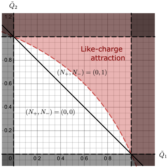
Figure 6: When $\tilde{q}_{-}>1$ (here $\tilde{q}_{-}=1.8$) the stability region in white does intersect the region of possible like-charge attraction in red defined by (42). The effective interaction can change from a repulsive one (white region) to an attractive one (red region). The greyed zone is forbidden by the stability condition (14).

Since the hyperbola that delimits the like-charge attraction region has asymptotes at $\tilde{Q}_{1}=\tilde{q}_{-}$ and $\tilde{Q}_{2}=\tilde{q}_{-}$, we deduce that the larger $\tilde{q}_{-}$ is, the larger the like-charge attraction region will be. But the maximum value for $\tilde{q}_{-}$ is $q_{-}/q_{+}$. Therefore to increase the possibility of like-charge attraction the ratio $q_{-}/q_{+}$ should be as large as possible. The charge-asymmetry is essential to observe the like-charge phenomenon. In the case of a charge-symmetric plasma of point particles, no like-charge attraction is observed.

The analysis for the case of negative guest charges is obtained from the previous one by interchanging the roles of $q_{-}$ and $q_{+}$. For that situation it is convenient to define $\hat{Q}_{1,2}=\beta q_{+}Q_{1,2}/2$ and $\hat{q}_{+}=\beta q_{+}^{2}/2$. The possibility of like charge attraction is when

$$(\hat{Q}_{1}+\hat{q}_{+})(\hat{Q}_{2}+\hat{q}_{+})<\hat{q}_{+}(-1+\hat{q}_{+})$$ (45)

which is only possible if $\hat{q}_{+}>1$. This situation can only be achieved if $q_{+}>q_{-}$ because the stability condition restricts $\hat{q}_{+}\in[0,q_{+}/q_{-})$. Therefore, in general, it is only possible to have like-charge attraction between one type of charges: positives if $q_{-}>q_{+}$ or the negative ones if $q_{+}>q_{-}$, but not both at the same time. So, the like-charge attraction phenomenon can occur when the point guest charges are screened by the ions of larger valency of the plasma.

All the previous analysis is restricted to the case of point particles, which is the reason to restrict the values of the charges to the stability region. To study the possibility of like-charge attraction beyond the stability region, it is necessary to introduce a non-electric short-distance repulsive potential between charges. This breaks downs the scale invariance of the pair potential and invalidates our analysis. The study of the region outside the stability regime requires special techniques ^{43, 46}, and the properties of the system change drastically compared to the case of point particles in the stability region. Therefore we will not speculate here on what could happen beyond the stability region.

3.4 Repulsion of charges of opposite sign?

A complementary question to the like-charge attraction dilemma is whether is it possible for opposite charges to repel each other? The answer is no, at least in the stability regime. This is because there are no changes in the effective interaction from the bare Coulomb potential if the charges have opposite signs. Indeed, suppose that $Q_{1}>0$ and $Q_{2}<0$, with $Q_{1}+Q_{2}>0$. For the effective potential $G_{Q_{1}Q_{2}}$ to change from the bare Coulomb interaction to a different form, it is needed that $\tilde{Q}_{1}+\tilde{Q}_{2}>1$. But this implies that $\tilde{Q}_{1}>1+|\tilde{Q}_{2}|>1$. Therefore $\tilde{Q}_{1}$ will be outside the stability region for this to occur. In conclusion, the effective interaction between oppositely charged particles behaves always as the bare attractive Coulomb potential at short distances $G_{Q_{1}Q_{2}}(r)\sim-Q_{1}Q_{2}\ln r$.

4 Conclusion

We have reviewed the mechanism of like-charge attraction in 1d and 2d exactly solvable Coulomb systems. Although the technical details differ depending on the dimension, the key mechanism is a three-body interaction between the two like-charges and an oppositely charged ion of the electrolyte or plasma. The charge asymmetry of the plasma increases the like-charge attraction effect. These 1d and 2d models provide a strong base to understand this intriguing phenomenon in 3d systems. In particular, like-charge attraction for parallel plates in an electrolyte in three dimensions has been put in evidence in the strong coupling regime and explained ¹³ using the one-single particle picture presented in the 1d model in section 2. This has important practical applications, for example in understanding the cement cohesion ⁴⁷.

This work was supported by Fondo de Investigaciones, Facultad de Ciencias, Universidad de los Andes INV-2021-128-2267. I thank Lucas Varela, Sergio Andraus, and Emmanuel Trizac for interesting discussions.

References

- 1 N. Ise, T. Okubo, M. Sugimura, K. Ito, H. J. Nolte, The Journal of Chemical Physics 1983, 78, 536–540.
- 2 Larsen A., Grier D., Nature 1997, 385, 230–233.
- 3 N. Grønbech-Jensen, K. M. Beardmore, Ph. Pincus, Physica A 1998, 261, 74–81.
- 4 P. Linse, V. Lobaskin, Phys. Rev. Lett. 1999, 83, 4208–4211.
- 5 J. C. Neu, Phys. Rev. Lett. 1999, 82, 1072–1074.
- 6 E. Trizac, J.-L. Raimbault, Phys. Rev. E 1999, 60, 6530–6533.
- 7 E. Trizac, Phys. Rev. E 2000, 62, R1465–R1468.
- 8 T. M. Squires, M. P. Brenner, Phys. Rev. Lett. 2000, 85, 4976–4979.
- 9 I. Rouzina, V. A. Bloomfield, J. Chem. Phys 1996, 100, 9977–9989.
- 10 A. Yu. Grosberg, T. T. Nguyen, B. I. Shklovskii, Rev. Mod. Phys. 2002, 74, 329–345.
- 11 Y. Levin, Reports on Progress in Physics 2002, 65, 1577.
- 12 A. G. Moreira, R. R. Netz, Phys. Rev. Lett. 2001, 87, 078301.
- 13 L. Šamaj, E. Trizac, Phys. Rev. Lett. 2011, 106, 078301.
- 14 E. Trizac, L. Šamaj, Physics of Complex Colloids, IOS Press Ebooks, 2013, chapter Like-charge colloidal attraction: A simple argument, pp. 61–73.
- 15 A. Lenard, Journal of Mathematical Physics 1961, 2, 682–693.
- 16 S. F. Edwards, A. Lenard, Journal of Mathematical Physics 1962, 3, 778–792.
- 17 S. Prager, Adv. Chem. Phys. 1962, 4, 201.
- 18 D. S. Dean, R. R. Horgan, A. Naji, R. Podgornik, The Journal of Chemical Physics 2009, 130, 094504.
- 19 B. Jancovici, Phys. Rev. Lett. 1981, 46, 386–388.
- 20 A. Alastuey, B. Jancovici, J. Phys. France 1981, 42, 1–12.
- 21 M. Gaudin, J. Phys. France 1985, 46, 1027–1042.
- 22 F. Cornu, B. Jancovici, J. Stat. Phys. 1987, 49, 33–56.
- 23 L. Šamaj, I. Travěnec, J. Stat. Phys. 2000, 101, 713–730.
- 24 G. Téllez, E. Trizac, Phys. Rev. E 2015, 92, 042134.
- 25 L. Varela, G. Téllez, E. Trizac, Phys. Rev. E 2017, 95, 022112.
- 26 L. Varela, G. Téllez, E. Trizac, Phys. Rev. E 2021, 103, 042603.
- 27 L. Varela, S. Andraus, E. Trizac, G. Téllez, J. Phys.: Condensed Matter 2021, 33, 394001.
- 28 R. L. Stratonovich, Soviet Physics Doklady 1957, 2, 416.
- 29 J. Hubbard, Phys. Rev. Lett. 1959, 3, 77–78.
- 30 A. B. Zamolodchikov, Al. B. Zamolodchikov, Annals of Physics 1979, 120, 253–291.
- 31 C. Destri, H. J. De Vega, Nuclear Physics B 1991, 358 (1), 251–294.
- 32 Al. B. Zamolodchikov, International Journal of Modern Physics A 1995, 10 (08), 1125–1150.
- 33 S. Lukyanov, Al. Zamolodchikov, Nuclear Physics B 1997, 493, 571–587.
- 34 S. Lukyanov, Physics Letters B 1997, 408 (1), 192–200.
- 35 F. A. Smirnov, Form Factors in Completely Integrable Models of Quantum Field Theory, World Scientific, Singapore, 1992.
- 36 V. Fateev, S. Lukyanov, A. Zamolodchikov, Al. Zamolodchikov, Nuclear Physics B 1998, 516 (3), 652–674.
- 37 P. Baseilhac, M. Stanishkov, Nuclear Physics B 2001, 612 (3), 373 – 390.
- 38 L. Šamaj, Journal of Statistical Physics 2003, 111 (1), 261–290.
- 39 G. Téllez, Journal of Statistical Mechanics: Theory and Experiment 2005, 2005 (10), P10001–P10001.
- 40 L. Varela, G. Téllez, Journal of Statistical Mechanics: Theory and Experiment 2021, 2021 (8), 083206.
- 41 L. Šamaj, B. Jancovici, J. Stat. Phys. 2002, 106, 301–312.
- 42 L. Šamaj, J. Stat. Phys. 2005, 120, 125–146.
- 43 L. Šamaj, J. Stat. Phys. 2006, 124, 1179–1206.
- 44 G. Téllez, Europhys. Lett. 2006, 76 (6), 1186–1192.
- 45 J. P. Hansen, P. Viot, Journal of Statistical Physics 1985, 38 (5), 823–850.
- 46 G. Téllez, J. Stat. Phys. 2007, 126, 281–298.
- 47 A. Goyal, I. Palaia, K. Ioannidou, F.-J. Ulm, H. van Damme, Roland J.-M. Pellenq, E. Trizac, E. Del Gado, Science Advances 2021, 7 (32), eabg5882.