A non-parametric proportional risk model to assess a treatment effect in time-to-event data

Abstract

Time-to-event analysis often relies on prior parametric assumptions, or, if a non-parametric approach is chosen, Cox’s model. This is inherently tied to the assumption of proportional hazards, with the analysis potentially invalidated if this assumption is not fulfilled. In addition, most interpretations focus on the hazard ratio, that is often misinterpreted as the relative risk. In this paper, we introduce an alternative to current methodology for assessing a treatment effect in a two-group situation, not relying on the proportional hazards assumption but assuming proportional risks. Precisely, we propose a new non-parametric model to directly estimate the relative risk of two groups to experience an event under the assumption that the risk ratio is constant over time. In addition to this relative measure, our model allows for calculating the number needed to treat as an absolute measure, providing the possibility of an easy and holistic interpretation of the data. We demonstrate the validity of the approach by means of a simulation study and present an application to data from a large randomized controlled trial investigating the effect of dapagliflozin on the risk of first hospitalization for heart failure.

Keywords and Phrases: time-to-event analysis, risk, number needed to treat, treatment effect, hazard ratio

* Corresponding author: Kathrin Möllenhoff, eMail: kathrin.moellenhoff@hhu.de

1 Introduction

In medical research, time-to-event data measuring the time until a specific endpoint, e.g. the time until death or the time until occurrence of a particular disease, are very common. In 2022, nearly 1,000 articles including the phrase ”time-to-event” were collected on PubMed [1]. Therefore, proper analysis of this type of data is of great interest. Well known models include proportional hazard (PH) models like Cox’s PH model [2] or the Weibull PH model [3] and proportional odds (PO) models like the log-logistic model [3], resulting in a focus on the hazard ratio (HR) and the odds ratio (OR) as estimates for the treatment effect. This contradicts the preference of reporting the relative risk (RR) when analysing data given in form of $2\times 2$ contingency tables [4].

The RR is characterized by its easy interpretability: If two groups, say A and B, have a RR of $r$ for an event, then group A is $r$ times more likely to experience the event relative to group B. Consequently, a RR of $1$ means an equal risk for both groups. If $r$ larger than $1$, group A has a larger risk than group B, and vice versa if it is smaller than $1$ [5]. The RR should always be reported in combination with an absolute risk measure like the numbers needed to treat, to classify the relative measure. Once this has been done, even complex statistical results can be communicated easily [4].

The misinterpretation of the HR as a RR has a long tradition, starting with even basic literature using the two terms interchangeably [6, 7]. However, this is incorrect: both measures indicate the same direction in regards to the treatment effect and hence have similar interpretation, but are technically not the same [8]. The HR is a conditional measure, based on rates [9], while the RR is not. Therefore, the two values should be strictly distinguished and handled with care.

In addition, an increase in studies reporting non-proportional hazard rates has been noted in recent years [10], putting the PH assumption into question. More precisely, the Cox model and the underlying PH assumption have been criticized recently, as the PH assumption is only rarely assessed in practice, or, the model is even used regardless of the presence of non-proportional hazards [11].

It is well known that the OR approximates the RR if the event of interest has a low prevalence [4]. Otherwise, these measures do not coincide, which led to widespread misinformation in the past [12]. Additionally, just as the PH assumption, the PO assumption is sometimes not suitable. To fill in the gap of the estimation of the RR for time-to-event data Kuss and Hoyer recently proposed a parametric proportional risk (PPR) model for a two group situation as typically given in in randomized controlled trials by using the exponentiated-uniform distribution [13]. This circumvents the problem of the incorrect interpretation of the HR and the OR, respectively.

Based on this idea, this paper proposes a non-parametric proportional risk (NPPR) estimator for the RR that is easy to implement, robust and particularly independent of the underlying cumulative distribution function. For the construction the Kaplan-Meier estimator [14] is used, allowing for the inclusion of right censored data. In addition to a relative risk measure, an absolute measure is needed to enable a holistic interpretation of the data [15]. Therefore, estimators for the risk difference and the number needed to treat are derived from the NPPR estimator.

The paper is structured as follows: First, we introduce the NPPR model and show how to estimate the treatment effect, given by the mean RR over time. Using this we then present a formula for the risk difference and the number needed to treat. Afterwards, we report a small simulation study that compares the NPPR estimator to the RR estimated by applying the PPR model. Finally, the practical usability of the model is illustrated by its application to data from the DAPA-HF trial [16], a large randomized controlled trial (RCT) investigating the effect of dapagliflozin on the risk of first hospitalization for heart failure.

2 Methodology

2.1 The non-parametric proportional risk (NPPR) model

We consider a situation with two groups, in terms of RCTs given by a treatment (indexed by $1$) and a control (indexed by $0$) group, respectively. The corresponding (unknown) cumulative distribution functions (CDFs) describing the probability of having experienced the outcome of interest up to a specific time point, are assumed to be proportional. This implies that their ratio, the RR, is constant over time, which we denote as proportional risk (PR) assumption.

Let $F_{1}$ and $F_{0}$ denote the corresponding unknown CDFs in the treatment and control group, respectively. Given the PR assumption evaluating the ratio of probabilities at any time point $t\geq 0$ (provided $F_{0}(t)\neq 0$), yields a treatment effect of

$$\frac{F_{1}(t)}{F_{0}(t)}=r$$

for a constant $r>0$. From this we define $\beta\in\mathbb{R}$ so that the equation

$$\exp\left(-\beta\right)=\frac{F_{1}(t)}{F_{0}(t)}=r$$

holds. Solving for $\beta$ we obtain

$$\beta \coloneqq-\log\left(\frac{F_{1}(t)}{F_{0}(t)}\right).$$ (1)

Moving to the log scale allows for a more symmetric interpretation of $\beta$. More precisely, a positive $\beta$ corresponds to a positive treatment effect, a negative $\beta$ to a negative one and $\beta=0$ to no effect, respectively. The main goal is to estimate $\beta$ without any parametric assumptions on the CDFs. Therefore, we estimate $F_{1}$ and $F_{0}$ by means of the non-parametric Kaplan-Meier estimators $\hat{S}_{1}$, $\hat{S}_{0}$, using the relationship between CDFs and their corresponding survival functions. The resulting estimated CDFs will be denoted by $\hat{F}_{i}=1-\hat{S}_{i}$, $i=0,1$. As the underlying data are possibly right censored, we need this slightly more complicated method of estimation instead of using the empirical CDFs.
Let $T_{1}$ and $T_{0}$ be the ordered sets of event time points for the two groups. We set $\tilde{t}_{min}=\max(\min(T_{1}),\min(T_{0}))$ and $\tilde{t}_{max}=\min(\max(T_{1}),\max(T_{0}))$. By defining

$$\tilde{T}=\left(t\mid t\in T_{1}\text{ or }t\in T_{0},\ \tilde{t}_{min}\leq t\leq\tilde{t}_{max}\right)$$

we restrict the time interval such that $\beta$ can be evaluated properly. Of note, tied observations are retained in $T_{1}$, $T_{0}$ and $\tilde{T}$ for later inclusion. Inserting the estimated CDFs instead of the true unknown CDFs in equation (1) for any $t$, $\tilde{t}_{min}\leq t\leq\tilde{t}_{max}$, yields a (time-dependent) estimator $\hat{\beta}_{t}$ for $\beta$.

To arrive at a single estimate for $\beta$, we compute a weighted mean of the $\hat{\beta}_{t}$ where the weights are derived from their variance. Precisely, as the Kaplan-Meier estimator is asymptotically normally distributed with a variance which can be approximated by Greenwood’s formula [17], we estimate the variance of $\hat{\beta}_{t}=-\log\left(\frac{\hat{F}_{1}(t)}{\hat{F}_{0}(t)}\right)=-\log\big{(}\hat{F}_{1}(t)\big{)}+\log\big{(}\hat{F}_{0}(t)\big{)}$ for every $t\in\tilde{T}$ by applying the delta method [18] to $\log(\hat{F}_{i}(t))$, $i=0,1$. This yields

$$\hat{\sigma}^{2}_{i}(t)\coloneqq\mbox{\sl Var}\ \big{(}\log(\hat{F}_{i}(t))\big{)}=\frac{1}{\hat{F}_{i}(t)^{2}}\mbox{\sl Var}\ \big{(}\hat{S}_{i}(t)\big{)},\ \ \ i=0,1.$$

Since $\hat{F}_{1}(t)$ and $\hat{F}_{0}(t)$ are independent and consequently their covariance is equal to $0$, we define the weight function by

$$\omega(t)\coloneqq\mbox{\sl Var}\ \big{(}\hat{\beta}_{t}\big{)}=\frac{1}{\hat{F}_{1}(t)^{2}}\mbox{\sl Var}\ \big{(}\hat{S}_{1}(t)\big{)}+\frac{1}{\hat{F}_{0}(t)^{2}}\mbox{\sl Var}\ \big{(}\hat{S}_{0}(t)\big{)}$$

for $t\in\tilde{T}$. Consequently, with $W:=\sum_{t\in\tilde{T}}\frac{1}{\omega(t)}$, a non-parametric estimator of $\beta$, the NPPR estimator, is defined by

$$\hat{\beta}=\frac{1}{W}\sum_{t\in\tilde{T}}\frac{1}{\omega(t)}\hat{\beta}_{t}=-\frac{1}{W}\sum_{t\in\tilde{T}}\frac{1}{\omega(t)}\log\left(\frac{\hat{F}_{1}(t)}{\hat{F}_{0}(t)}\right).$$ (2)

As stated above, tied observations were retained in $\tilde{T}$. Therefore, if an event time point $t^{\prime}$ is included $m$ times over both $T_{1}$ and $T_{0}$, the term $\frac{1}{\omega(t^{\prime})}\hat{\beta}_{t^{\prime}}$ is also included $m$ times in the sum in (2). A visualization of the situation is given in Figure 1. Also, the estimator does in general estimate the mean RR over time. This holds even if the PR assumption is violated. In this case the estimator still provides a summary of the RR.

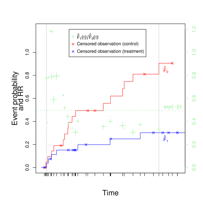
Figure 1: Visualization of the NPPR estimator. The size of the crosses symbolises the weight given to the respective estimated RR at this time point. The larger the cross, the larger the weight. For a visualization on a logarithmic scale we refer to the supplementary material (Figure A).

2.2 Risk difference and number needed to treat

In order to ensure a holistic interpretation of the data, an absolute measure is needed in addition to the relative measure provided by the RR. The risk difference for the unknown true CDFs is defined by

$$RD(t)=F_{0}(t)-F_{1}(t)$$

for $t\geq 0$. Using the PR assumption, we can write $F_{1}(t)=\exp(-\beta)F_{0}(t)$ and substitute $F_{1}(t)$ in the formula. This yields

$$RD(t)=\big{(}1-\exp(-\beta)\big{)}F_{0}(t).$$

Now we can insert the estimated CDF $\hat{F}_{0}$ corresponding to the Kaplan-Meier estimator $\hat{S}_{0}$ and the NPPR estimator $\hat{\beta}$ obtained by (2). The resulting estimator of the risk difference is defined by

$$\widehat{RD}(t)=\big{(}1-\exp(-\hat{\beta})\big{)}\hat{F}_{0}(t)$$

for $\tilde{t}_{min}\leq t\leq\tilde{t}_{max}$. Of note, this still does depend on the time $t$ and given the PR assumption monotonically decreases if $\exp(-\hat{\beta})<1$ and increases if $\exp(-\hat{\beta})>1$, respectively.

The number needed to treat is defined as the reciprocal of the risk difference. Therefore an estimator is given by

$$\widehat{NNT}(t)=\frac{1}{\widehat{RD}(t)}=\frac{1}{\big{(}1-\exp(-\hat{\beta})\big{)}\hat{F}_{0}(t)}.$$

3 Simulation study

3.1 Setting and data generation

In order to evaluate the performance of the NPPR estimator compared to an alternative method we conducted a simulation study. As a competitor we chose the PPR model for estimating the RR. The PPR model is based on the exponentiated-uniform (EU) distribution [13], and the corresponding CDFs are given by

$$F_{EU,i}(t)=\left(\theta_{i}t\right)^{\alpha},\ \ \ t\leq\frac{1}{\theta_{i}},\text{ for }i=0,1,$$

in which the shape parameter $\alpha>0$ is assumed to be the same for both the treatment and the control group and the scale parameters $\theta_{i}>0$, $i=0,1$, are assumed to be group-specific. By calculating maximum likelihood (ML) estimates using the R function optim for $\theta_{i}$, $i=0,1$, and $\alpha$, the estimated RR is given by

$$\widehat{RR}_{EU}=\left(\frac{\hat{\theta_{1}}}{\hat{\theta_{0}}}\right)^{\hat{\alpha}}.$$

Outcomes of the simulation study were bias, mean squared error (MSE) and empirical coverage of the estimated RR, respectively. Additionally, we evaluated numerical robustness in terms of the number of converged simulation runs. All analyses have been done using R version 4.2.2.

The simulation setting was inspired by the DAPA-HF trial discussed as a case study example in Section 4. We simulated both a PR and a PH situation with different true underlying effects for the RR or the HR, respectively. For the generation of data satisfying the PR assumption the PPR model was used. For a PH scenario we used a Weibull PH model. The corresponding CDFs are given by

$$F_{Weib,i}(t)=\begin{cases}1-e^{-\left(\frac{t}{\lambda_{i}}\right)^{k}}&\text{ for }x\geq 0\\ 0&\text{ for }x<0\end{cases}\text{ for }i=0,1.$$

Here, $k>0$ is the shape parameter, which is assumed to be equal for both groups, and $\lambda_{i}$, $i=0,1$, are the group specific scale parameters. In both scenarios we used the parameters obtained from the placebo group of the data set as underlying truth to simulate data for the reference group, where we chose true underlying parameters $\beta=0,\ 0.5,\ 0.25,\ -0.25,\ -0.5$ which correspond to a RR/HR equal to $1,\ 0.607,\ 0.779,\ 1.284$ and $1.649$ (see Figure 2 for a visualization of the RRs over time). All configurations used for the simulations are summarized in Table 1. For a visualization of the CDFs we refer to Figure B in the supplementary material.

To achieve different amounts of censoring ($30\%$, $50\%$ and $70\%$) we simulated censoring times from an appropriate uniform distribution. For each of these combinations we varied the number of study participants ($50$, $100$ and $500$). All simulation results were obtained from simulating $1,000$ studies. Combining both the PR and PH cases resulted in $90$ simulation scenarios representing a situation with no, a realistic and a more extreme effect on both sides of the null effect. In all cases we first drew the group assignment using inverse transformation sampling of a binomial distribution with probability $p=0.5$. Afterwards, corresponding to the declared underlying true effect, we drew survival times from the the PPR model or the Weibull PH model, again using inverse transformation sampling.

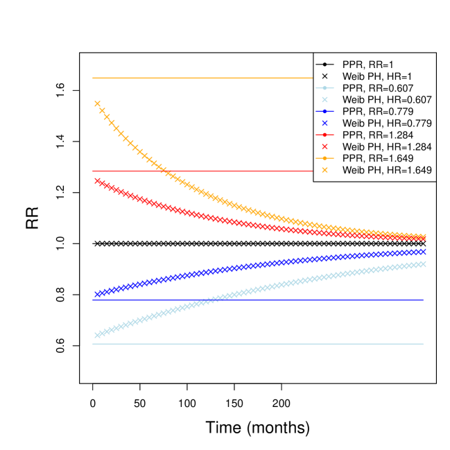
Figure 2: RR of the PPR model in comparison with the RR of the Weibull PH model over time.

Given the censoring rate we then drew censoring times from the uniform distribution - for the specific parameters see the supplementary material (Table A) - for each participant. Finally, the observed time of each individual was defined as minimum of the survival and censoring time and the status adjusted accordingly.

Table 1: Parameters of the PPR model and the Weibull PH model corresponding to the true underlying effects for all different cases.

True underlying effect		Parameters
		PPR			Weibull PH
$\beta$	RR/HR	$\alpha$	$\theta_{1}$	$\theta_{0}$	$k$	$\lambda_{1}$	$\lambda_{0}$
0	1	0.859	0.009	0.009	0.916	88.296	88.296
0.5	0.607	0.859	0.005	0.009	0.916	145.575	88.296
0.25	0.779	0.859	0.007	0.009	0.916	113.374	88.296
-0.25	1.284	0.859	0.012	0.009	0.916	68.765	88.296
-0.5	1.649	0.859	0.016	0.009	0.916	53.554	88.296

3.2 Estimation

We compared the NPPR estimator with the RR estimated using the PPR model only if for the underlying data generating model the PR assumption was satisfied. For the performance of the PPR model in case of PH data we refer to Kuss & Hoyer [13]. Of note, the Weibull PH model violates the PR assumption. However, when applying the NPPR estimator we still assumed a PR by treating the true value of the HR as true value of the RR and proceeded with the analysis accordingly. This was done to examine the behavior of the NPPR model, if the PR assumption does not hold, which can be the case in practical applications. Further, as there is no true underlying constant RR we chose the HR in order to mimic the often seen practice to use the RR and the HR interchangeably [8].

Of note, it might happen that all events of one group have already occurred before the first event of the other group occurs. Under these circumstances, or when all participants were censored, $\tilde{T}$ might be empty. Then the NPPR estimator is not defined. These cases are few in numbers and were excluded from further analysis. Similarly, for realistic results, datasets yielding estimates obtained by the PPR model of an absolute effect ($|-\log(\widehat{RR}_{EU})|$) larger than $3$ were removed. This choice was informed by an analysis of the simulated data with Cox’s PH model, that is not shown here. Precisely, limiting the analysis to estimated HRs smaller than $20$ ($\approx\exp(3)$) was the most conservative way to exclude estimations suffering from obvious numerical issues. Of note, the NPPR estimator exceeded this limit in no case.

Finally, we again refer to the results presented by Kuss & Hoyer [13] for the reversed situation of Cox’s PH model used in case of PR data.

3.3 Results

In the following we will present the results of the simulation study. As the NPPR model directly estimates $\hat{\beta}=-\log(\widehat{RR})$ we transform the estimate $\widehat{RR}_{EU}$ obtained by the PPR model to $-\log(\widehat{RR}_{EU})$ for an easier comparability. Table 2 and Table 3 display the bias and the MSE for the different scenarios, respectively. For details on the coverage and the numerical robustness we refer to the supplementary material (Tables B-E).

For a quick introduction Figure 3 displays a comparison between the estimated $\hat{\beta}$ (NPPR) and $-\log(\widehat{RR}_{EU})$ (PPR) for a censoring rate of $50\%$ and $500$ participants if the PR assumption is fulfilled.

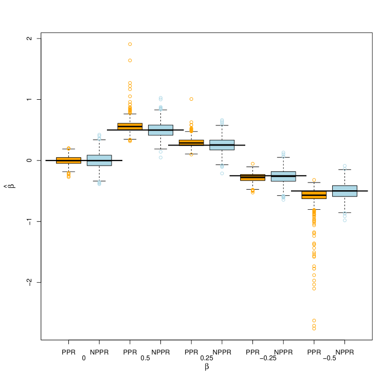
Figure 3: Comparison of boxplots for the estimated $\hat{\beta}$ (NPPR) and $-\log(\widehat{RR}_{EU})$ (PPR) for different choices of $\beta$ if the PPR model is the underlying model, each in case of $500$ participants and $50\%$ censoring rate. Horizontal bars indicate the true underlying effect. Boxplots for $30\%$ and $70\%$ censoring rates and for the PH cases are displayed in the supplementary material (Figures C-G).

If the true underlying effect $\beta$ equals $0$, the NPPR estimator has a larger IQR than the PPR model with equal median. In all remaining cases the median is closer to the true value, while the IQR is still a bit larger. We observe that the NPPR estimator produces fewer outliers compared to the PPR model. Similar findings are achieved for situations with a censoring rate of $30\%$ and only in case of a high censoring rate, that is $70\%$, the number of outliers is comparable (see supplementary material Figure C-D).

3.3.1 Bias

Tables 2 and 3 depict the bias. It turns out that if the censoring rate is $50\%$ or smaller the NPPR estimator consistently outperforms the PPR model for all underlying effects but $\beta=0$. This also holds for almost all other configurations, with only a few exceptions. For instance, considering a censoring rate of $70\%$ and a true effect of $\beta=0.25$ or $\beta=-0.25$ the bias of the NPPR model is for some configurations slightly larger than the one presented by the PPR model. If there is no treatment effect, i.e. $\beta=0$, the difference in biases mostly ranges in order of a magnitude of $0.004$, which is very small. Only in case of a rather high amount of censoring, i.e. $70\%$, and a small sample size of $50$ participants this difference, given by $0.023$, is noticeably larger.

If the Weibull PH model is the true underlying model, the NPPR estimator has a slightly larger bias when trying to approximate the HR. It still never ecxeeds $0.177$. The negative values of $\beta$ tend to be overestimated, while the positive ones are underestimated. This behavior is consistent with the trend observed for the RR over time (see Figure 2). We note that the NPPR estimator is more precise for smaller censoring rates and a higher number of participants, as expected. Overall it performs satisfactory and reliable in all cases under consideration.

Table 2: Bias and MSE of $\hat{\beta}$ (NPPR) and $-\log(\widehat{RR}_{EU})$ (PPR) if the PPR model is the true underlying model.

Effect	Censoring ($\%$)	Participants	Bias		MSE
			NPPR	PPR	NPPR	PPR
0.00	30	500	0.002	-0.011	0.010	0.120
0.00	30	100	0.003	0.018	0.050	0.303
0.00	30	50	0.010	-0.006	0.106	0.424
0.00	50	500	0.000	0.000	0.016	0.005
0.00	50	100	-0.005	0.002	0.079	0.037
0.00	50	50	0.006	0.008	0.156	0.140
0.00	70	500	-0.005	-0.003	0.027	0.016
0.00	70	100	0.006	0.006	0.135	0.084
0.00	70	50	-0.040	-0.017	0.270	0.187
0.50	30	500	0.003	0.204	0.013	0.175
0.50	30	100	-0.004	0.314	0.063	0.458
0.50	30	50	0.014	0.384	0.115	0.592
0.50	50	500	0.001	0.065	0.016	0.016
0.50	50	100	0.001	0.152	0.079	0.118
0.50	50	50	-0.029	0.204	0.171	0.284
0.50	70	500	0.004	0.006	0.029	0.019
0.50	70	100	0.006	0.027	0.146	0.091
0.50	70	50	-0.043	0.007	0.298	0.265
0.25	30	500	-0.006	0.087	0.011	0.130
0.25	30	100	0.003	0.107	0.052	0.407
0.25	30	50	-0.009	0.153	0.106	0.391
0.25	50	500	0.002	0.041	0.015	0.008
0.25	50	100	0.002	0.112	0.072	0.091
0.25	50	50	0.008	0.139	0.159	0.197
0.25	70	500	0.002	0.001	0.026	0.014
0.25	70	100	-0.015	0.000	0.127	0.084
0.25	70	50	-0.022	0.012	0.285	0.207
-0.25	30	500	0.005	-0.139	0.011	0.188
-0.25	30	100	-0.001	-0.136	0.059	0.377
-0.25	30	50	0.000	-0.166	0.106	0.525
-0.25	50	500	-0.013	-0.032	0.015	0.006
-0.25	50	100	0.006	-0.094	0.076	0.091
-0.25	50	50	0.002	-0.116	0.161	0.162
-0.25	70	500	0.002	0.000	0.028	0.017
-0.25	70	100	0.006	0.006	0.142	0.091
-0.25	70	50	0.038	-0.003	0.280	0.239
-0.50	30	500	0.012	-0.227	0.011	0.222
-0.50	30	100	-0.010	-0.323	0.065	0.411
-0.50	30	50	-0.009	-0.297	0.135	0.552
-0.50	50	500	-0.002	-0.097	0.017	0.052
-0.50	50	100	0.005	-0.184	0.076	0.145
-0.50	50	50	-0.009	-0.230	0.169	0.258
-0.50	70	500	-0.003	-0.006	0.031	0.019
-0.50	70	100	0.019	-0.006	0.157	0.098
-0.50	70	50	0.045	-0.051	0.313	0.240

Table 3: Bias and MSE of $\hat{\beta}$ obtained by the NPPR estimator if the Weibull PH model is the true underlying model.

Effect	Censoring ($\%$)	Participants	Bias	MSE
0.00	30	500	0.001	0.011
0.00	30	100	-0.001	0.052
0.00	30	50	-0.002	0.096
0.00	50	500	0.000	0.015
0.00	50	100	-0.009	0.079
0.00	50	50	0.003	0.163
0.00	70	500	0.006	0.027
0.00	70	100	0.015	0.136
0.00	70	50	-0.020	0.292
0.50	30	500	-0.158	0.036
0.50	30	100	-0.156	0.078
0.50	30	50	-0.177	0.130
0.50	50	500	-0.124	0.032
0.50	50	100	-0.122	0.100
0.50	50	50	-0.125	0.212
0.50	70	500	-0.100	0.040
0.50	70	100	-0.113	0.164
0.50	70	50	-0.128	0.346
0.25	30	500	-0.080	0.017
0.25	30	100	-0.096	0.057
0.25	30	50	-0.090	0.109
0.25	50	500	-0.068	0.018
0.25	50	100	-0.072	0.079
0.25	50	50	-0.070	0.170
0.25	70	500	-0.051	0.031
0.25	70	100	-0.055	0.141
0.25	70	50	-0.052	0.281
-0.25	30	500	0.082	0.016
-0.25	30	100	0.071	0.055
-0.25	30	50	0.087	0.110
-0.25	50	500	0.058	0.018
-0.25	50	100	0.052	0.079
-0.25	50	50	0.065	0.167
-0.25	70	500	0.046	0.030
-0.25	70	100	0.085	0.172
-0.25	70	50	0.063	0.339
-0.50	30	500	0.161	0.037
-0.50	30	100	0.175	0.080
-0.50	30	50	0.147	0.129
-0.50	50	500	0.136	0.032
-0.50	50	100	0.133	0.090
-0.50	50	50	0.140	0.188
-0.50	70	500	0.097	0.040
-0.50	70	100	0.106	0.156
-0.50	70	50	0.140	0.340

3.3.2 MSE

Tables 2 and 3 also depict the observed MSE. If the PPR model was assumed to be the true model we note the same tendencies as seen with the bias. The NPPR estimator presents a smaller MSE for a low censoring rate of $30\%$ in all cases. Considering $50\%$ censoring it is overall smaller or equal to the one observed with the PPR model if $\beta\neq 0$ and for less than $500$ participants if $\beta=0.25$ or $\beta=-0.25$. The MSE of the NPPR estimator never exceeds $0.313$ (true value $\beta=-0.50$, $70\%$ censoring, $50$ participants). On the other hand, the PPR model shows a MSE up to $0.592$ (true value $0.50$, $30\%$ censoring, $50$ participants). If the Weibull PH model is the true underlying model, the NPPR estimator presents a similar MSE as for the PR case. It never exceeds $0.346$ (true value $\beta=0.50$, $70\%$ censoring, $50$ participants). Overall we conclude that the MSEs corresponding to the NPPR model show promising behavior, also in case of a violation of the PR assumption.

3.3.3 Coverage

As in general the covariances $\text{\rm Cov}(\hat{\beta}_{t},\hat{\beta}_{t^{\prime}})$ for $t\neq t^{\prime}$, $t,t^{\prime}\in\tilde{T}$, are unknown and it is therefore impossible to determine the variance of $\hat{\beta}$ in (2) directly, the confidence intervals for the NPPR estimator were constructed according to the percentile bootstrap approach [19]. Precisely, for each study with $n$ participants we drew an independent sample with replacement of size $n$ from the simulated study. The group assignment and status were not changed throughout. From this sample $\hat{\beta}^{*}$ was estimated again using the NPPR estimator as described in Section 2. This procedure was repeated $500$ times, yielding $\hat{\beta}^{*(1)},\ldots,\hat{\beta}^{*(500)}$. From these values, the empirical $2.5\%$-quantile and $97.5\%$-quantile, respectively, were determined, defining the corresponding $95\%$ confidence interval. For the PPR model we used the multivariate delta method [20] to construct the confidence intervals.

Details on the coverage for each simulated case are presented in the supplementary material (Tables B-C). In general, if the PPR model is the true underlying model, the simulated coverage of the confidence interval for the NPPR estimator is very close to the desired confidence level of $95\%$. It rarely falls below this value, the smallest value is given by $93.7\%$ and the highest coverage is given by $98.2\%$. The latter is reached in case of a true effect of $-0.25$, $70\%$ censoring and $50$ participants, which underlines the fact that confidence intervals become rather conservative if the number of events is low.

Overall the PPR model performs comparably. The smallest simulated coverage equals $89.4\%$ and is observed in case of a true effect equal to $0.50$ with a censoring rate of $30\%$ and $100$ participants. If the Weibull PH model is the true underlying model the coverage of the HR, approximated by the RR, is overall too low, which is a direct consequence of the violated PR assumption. However, we conclude that also in this case, for most of the configurations the approximation of the $95\%$-level is still rather precise.

3.3.4 Numerical Robustness

The NPPR estimator proves to be overall robust, independent of the true underlying model. Assuming the PPR model, failures (less than 16 in 1,000 simulation runs) were only observed in $5$ of the $45$ scenarios. This is also true for the Weibull PH model as underlying model, where the NPPR model only failed a very few times ($<10$), occurring only in case of a high censoring rate of $70\%$ and a small sample size of $50$ participants. Concerning the numerical robustness, the PPR model is clearly outperformed by the NPPR model , showing a higher robustness in almost every case. For the sake of brevity, details are deferred to the supplementary material (Tables D-E).

4 Case study: DAPA-HF trial

To illustrate the NPPR estimator, we use data from the DAPA-HF trial [16]. This randomized, double-blind, placebo-controlled trial evaluated dapagliflozin, a sodium glucose cotransporter-2 (SGLT-2) inhibitor, for reducing severe cardiovascular outcomes in patients with heart failure and reduced ejection fraction. In 410 sites in 20 countries, 4,744 patients were treated for a median observation time of 18.2 months. Here we report the results for the trial’s primary outcome, time to worsening heart failure or cardiovascular death. Overall, 385 (out of 2,373) patients experienced this outcome in the treatment group, but 500 (out of 2371) in the control group.

As we had no access to the original data, we digitized the Kaplan-Meier estimates from the original paper by the open software tool WebPlotDigitizer, version 3.8 [21] and extracted the data by using the algorithms and R tools of Guyot et al. [22]. In order to validate this extraction process, we calculated a hazard ratio (with 95% CI) from the extracted data given by 0.745 [0.653, 0.851], which is essentially the same as the hazard ratio and its CI in the original paper, which was 0.74 [0.65, 0.85].

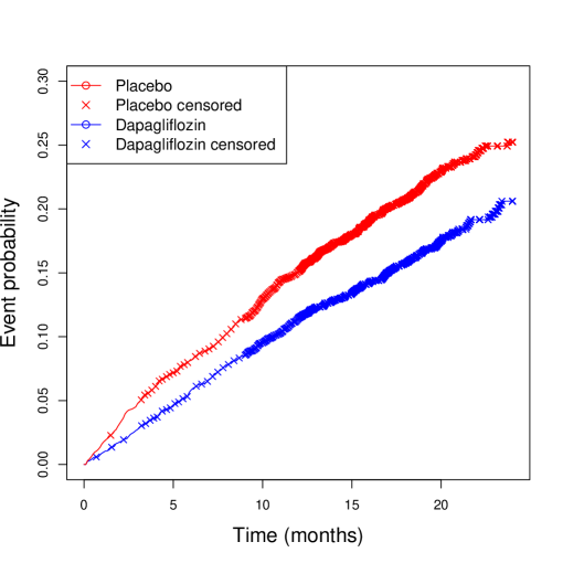
Figure 4: Event probability of the primary outcome of interest and event time points during the DAPA-HF trial estimated with the Kaplan-Meier estimator.

Figure 4 displays the estimated CDFs from the DAPA-HF trial. The assumption of PR seems to be reasonable. Using the method described in Section 2 we obtain $\hat{\beta}=0.320$ ($95\%$CI $\left[0.178,0.454\right]$), which corresponds to a RR of $0.726$ ($95\%$CI $\left[0.635,0.837\right]$). The patients in the treatment group are therefore only $72.6\%$ at risk of worsening heart failure or cardiovascular death relative to the patients in the placebo group. Confidence intervals were estimated using the bootstrap as described in Section 3.3.3. To visualize the estimation process Figure 5 a) shows the estimated $\hat{\beta}_{t}$ for each event time point. The weighted mean defining the NPPR estimator as defined in (2) is displayed by the solid line. The weights at each event time point are shown in Figure 5 b).

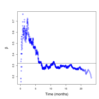
a) b)

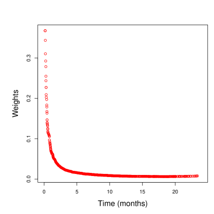
Figure 5: a) Estimated $\hat{\beta}_{t}$ for the DAPA-HF trial at every event time point. The estimated $\hat{\beta}$ overall is displayed by the line. b) Weights at every event time point.

The estimated number needed to treat quickly decreases over time, likely due to the small number of reported events in the study. For instance, at the time point $t=10$ only $29$ ($28.120$ estimated, $95\%$ CI $\left[19.256,53.947\right]$) patients treated with dapagliflozin would prevent one death relative to the placebo treatment. A detailed visualization of the number needed to treat are shown in Figure H in the supplementary material.

5 Discussion and conclusion

In this paper we proposed a non-parametric proportional risk model to assess a treatment effect in case of a two-group situation. Thereby we solved the conceptional problems the HR and OR have shown in the past without losing the advantages of a non-parametric estimation method. By deducing the number needed to treat from the model, we further provide an absolute measure in addition to the estimated RR. As no further specification beyond the PR assumption is necessary, the model is broadly applicable and provides a promising tool for the analysis of numerous applications, ranging from preclinical toxicology studies to late phase clinical trials, as for instance RCTs.

Of course, the NPPR estimator comes along with some limitations. Up to this point the model contains only one (binary) variable and it is not possible to include further variables in the model. Moreover the consideration of continuous variables is a challenging problem, which demands some future work. Another drawback, especially if compared to the parametric model, is the necessity of using bootstrap to calculate a confidence interval as a formula for the variance of the estimator is not available yet.

We demonstrated that the NPPR estimator shows a very good performance if the PR assumption is fulfilled. For small to moderate censoring rates it mostly outperforms the PPR model and is numerically more robust. If the PR assumption is not fulfilled it still shows satisfying behavior. However, if there are only few events, either due to high censoring rates or generally small sample sizes, problems can arise or even make an application impossible. In those cases, while still less robust, the PPR model can provide a better solution. The NPPR estimator in general estimates the mean RR over time. Therefore, applications outside of a PR scenario might also be of interest. Further, similarly to the discussion about the PH assumption required from Cox’s model, possible problems resulting from a violated PR assumption should be taken into consideration.

In summary, we strongly believe that the NPPR estimator is a useful addition to the existing tools for the analysis of time-to-event data, which not only circumvents the technical problems of the HR and the OR, respectively, but is also easy to interpret and comes along without an assumption on the underlying survival distribution.

Supplementary material

Supplementary material providing additional tables and figures can be found online. Corresponding R code, which can be used to reproduce the analysis of the case study and the simulation results, is available at https://github.com/LuciaAmeis/NPPR-model-for-time-to-event-data.

Funding

This work has been supported by the Research Training Group ”Biostatistical Methods for High-Dimensional Data in Toxicology” (RTG 2624, P7) funded by the Deutsche Forschungsgemeinschaft (DFG, German Research Foundation - Project Number 427806116).

References

- [1] PubMed. https://pubmed.ncbi.nlm.nih.gov/?term=time-to-event (accessed 24th of February 2023).
- Cox [1972] D.R. Cox. Regression models and life-tables. Journal of the Royal Statistical Society Series B Methodological, 34(2):187–220, 1972.
- Kleinbaum and Klein [2012] D. G. Kleinbaum and M. Klein. Survival analysis - a self-learning text. Statistics for Biology and Health. Springer Science Business Media, New York, 3. edition, 2012.
- Sistrom and Garvan [2004] C.L. Sistrom and C.W. Garvan. Proportions, odds, and risk. Radiology, 230(1):12–19, 2004.
- Rosner [2016] B. Rosner. Fundamentals of Biostatistic. Cengage Learning, Boston, MA, 2016. 8th Edition.
- Klein and Moeschberger [2003] J.P. Klein and M.L. Moeschberger. Survival Analysis Techniques for Censored and Truncated Data. Statistics for Biology and Health. Springer, 2003. 2nd Edition.
- Kalbfleisch and Prentice [2002] J.D. Kalbfleisch and R.L. Prentice. The Statistical Analysis of Failure Time Data. Wiley Series in Probability and Statistics. John Wiley & Sons, 2011, 2002. 2nd Edition.
- Sutradha and Austin [2018] R. Sutradha and P.C. Austin. Relative rates not relative risks: addressing a widespread misinterpretation of hazard ratios. Ann Epidemiol, 28(1):54–57, 2018.
- Hernán [2010] M.A. Hernán. The hazards of hazard ratios. Epidemiology, 21(1):13–15, 2010. Erratum in: Epidemiology, 22:134, 2011.
- Royston [2014] M.K Royston, P.and Parmar. An approach to trial design and analysis in the era of non-proportional hazards of the treatment effect. Trials, (15), 2014. Article number: 314.
- Jachno et al. [2019] K. Jachno, S. Heritier, and R. Wolfe. Are non-constant rates and non-proportional treatment effects accounted for in the design and analysis of randomised controlled trials? a review of current practice. BMC Med Res Methodol, (19), 2019. Article number: 103.
- Schwartz and Woloshin [1999] L.M. Schwartz and H.G. Woloshin, S. ad Welch. Misunderstandings about the effects of race and sex on physicians’ referrals for cardiac catheterization. N Engl J Med, 341(4):discussion 286–7, 1999.
- Kuss and Hoyer [2021] O. Kuss and A. Hoyer. A proportional risk model for time-to-event analysis in randomized controlled trials. Statistical Methods in Medical Research, 30(2):411–424, 2021.
- Kaplan and Meier [1958] E.A. Kaplan and P. Meier. Nonparametric estimation from incomplete observations. Journal of the American Statistical Association, 53(282):457–481, 1958.
- [15] The Academy of Medical Sciences. Sources of evidence for assessing the safety, efficacy and effectiveness of medicines. https://acmedsci.ac.uk/file-download/86466482 (2017, accessed 6th of March 2023).
- McMurray et al. [2019] J.J.V. McMurray, S.D. Solomon, S.E. Inzucchi, L. Køber, M.N. Kosiborod, F.A. Martinez, P. Ponikowski, M.S. Sabatine, I.S. Anand, J. Bĕlohlávek, M. Bøhm, C. Chiang, for the DAPA-HF Trial Committees et al., and Investigators. Dapagliflozin in patients with heart failure and reduced ejection fraction. The New England Journal of Medicin, 381(21):1995–2008, 2019.
- Breslow and Crowley [1974] N. Breslow and J. Crowley. A large sample study of the life table and product limit estimates under random censorship. The Annals of Statistics, 2(3):437–453, 1974.
- Oehlert [1992] G.W. Oehlert. A note on the delta method. The American Statistician, 46(1):27–29, 1992.
- Efron [1981] B. Efron. Censored data and the bootstrap. Journal of the American Statistical Association, 76(374):312–19, 1981.
- van der Vaart [1998] A.W. van der Vaart. Asymptotic Statistics. Cambridge Series in Statistical and Probabilistic Mathematics. Cambridge University Press, 1998.
- Rohatgi [2015, accessed 14th of September 2022] A. Rohatgi. WebPlotDigitizer. 2015, accessed 14th of September 2022. https://automeris.io/WebPlotDigitizer/.
- Guyot et al. [2012] P. Guyot, A. Ades, M.J. Ouwens, and et al. Enhanced secondary analysis of survival data: reconstructing the data from published kaplan-meier survival curves. BMC Med Res Methodol, 12:9, 2012.