Abstract

We provide a unified framework, applicable to a general family of convex losses and across binary and multiclass settings in the overparameterized regime, to approximately characterize the implicit bias of gradient descent in closed form. Specifically, we show that the implicit bias is approximated (but not exactly equal to) the minimum-norm interpolation in high dimensions, which arises from training on the squared loss. In contrast to prior work which was tailored to exponentially-tailed losses and used the intermediate support-vector-machine formulation, our framework directly builds on the primal-dual analysis of [29], allowing us to provide new approximate equivalences for general convex losses through a novel sensitivity analysis. Our framework also recovers existing exact equivalence results for exponentially-tailed losses across binary and multiclass settings. Finally, we provide evidence for the tightness of our techniques, which we use to demonstrate the effect of certain loss functions designed for out-of-distribution problems on the closed-form solution.

1 Introduction

The choice of loss function to optimize a model over training examples is an important cornerstone of the machine learning (ML) pipeline. This choice is particularly nuanced for the task of classification, which is evaluated by the 0-1 risk on test data. An elegant classical viewpoint is that training loss functions should be designed as continuous and optimizable surrogates [4, 61, 35, 51] to the 0-1 risk, as the training surrogate loss can often be related to the test surrogate risk, and the test surrogate risk can in turn be related to the test 0-1 risk. However, the first part of this reasoning breaks down in the modern high-dimensional regime, where infinitely many solutions can achieve zero training loss, but the test risk widely varies across these solutions [60, 44].

The goal of this work is to provide a more transparent understanding of the impact of the training loss function on the eventual solution (and, thereby, its generalization) in this high-dimensional regime. Recent empirical and theoretical work provides a mixed and incomplete picture of the impact of loss. On one hand, large-scale empirical studies [25, 32, 17, 26] have shown that the less popular squared loss generates surprisingly competitive performance to the popular cross-entropy loss (the multiclass extension of the binary logistic loss). On the other hand, the cross-entropy loss (and, more generally, the family of exponentially-tailed losses [50, 28]) is the only one that admits a direct relationship with maximization of the worst-case training data margin, which often correlates with good generalization [3, 6]. The empirically more challenging task of out-of-distribution (OOD) generalization [37] yields further subtleties, with a diversity of loss functions that deviate significantly from this standard family of exponentially-tailed losses being recently designed and evaluated [47, 9, 38, 31, 57].

Even for linear models, a comprehensive theory for the impact of a general loss function on the ensuing solution (and, thereby, its generalization) is currently missing. While promising frameworks have been recently provided for the implicit bias of general losses through convex programming [27, 29], the properties of the implicit bias itself remain opaque. A separate recent line of work [40, 23, 56, 55, 10] shows that the squared loss and cross-entropy loss can yield identical solutions with high probability in high dimensions, complementing their aforementioned noticed similarities in empirical performance. In particular, both solutions are shown to exactly coincide with minimum-norm interpolation (MNI), which enjoys a closed-form expression and often generalizes well in high dimensions [5, 8, 21, 33, 41, 40]. However, these proof techniques are highly tailored to exponentially-tailed losses and in particular the intermediate support-vector-machine (SVM) formulation [50], leaving open the question of whether such equivalences can be proved for more general losses.

Our contributions:

In this paper we characterize the closed-form properties of the implicit bias of general convex losses arising from gradient descent in high dimensional linear models, by building on the primal-dual characterization of the implicit bias provided in [29]. In Section 2.1 we show (Proposition 1 and Theorem 1) that general convex losses in conjunction with gradient descent yield solutions that are approximately directionally close to minimum-norm interpolation (MNI) on binary labels in a sufficiently high-dimensional regime with high probability. Our approximation error term is a decreasing function of an “effective dimension” which also appears in sufficient and necessary conditions for exact equivalence between the SVM and MNI [23, 1]. In contrast to all prior literature that works with the SVM, our analysis directly leverages the primal-dual framework of [29], allowing us to recover the exact equivalence to MNI for exponentially-tailed losses [23] through an alternative proof technique. Our upper bounds on the approximation error utilize a novel sensitivity analysis of the dual implicit bias in high dimensions and are applicable to general convex losses.

In Section 3.1 we extend our framework to the multiclass setting using the general loss function formulation in [22] (originally proposed for exponential losses to extend AdaBoost to the multiclass setting), showing along the way that the primal-dual analysis in [29] can be naturally extended to the multiclass setting. We also treat the cross-entropy loss separately and provide an alternative proof of exact equivalence to MNI that is conceptually simpler than the one provided in [55], requiring no transformation of the implicit-bias dual in [29] other than a rescaling.

Finally, in Section 4 we provide partial evidence for the tightness of our arguments. In Proposition 3 we show that the conditions for exact equivalence in Theorem 1 are not only sufficient but necessary. We leverage this converse result to make an interpretable link between the popular techniques of importance-weighting on heavy-tailed losses [57] and vector-scaling of exponential losses [31] and a type of cost-sensitive interpolation, thereby providing a possible explanation for their success in addressing OOD generalization.

1.1 Related work

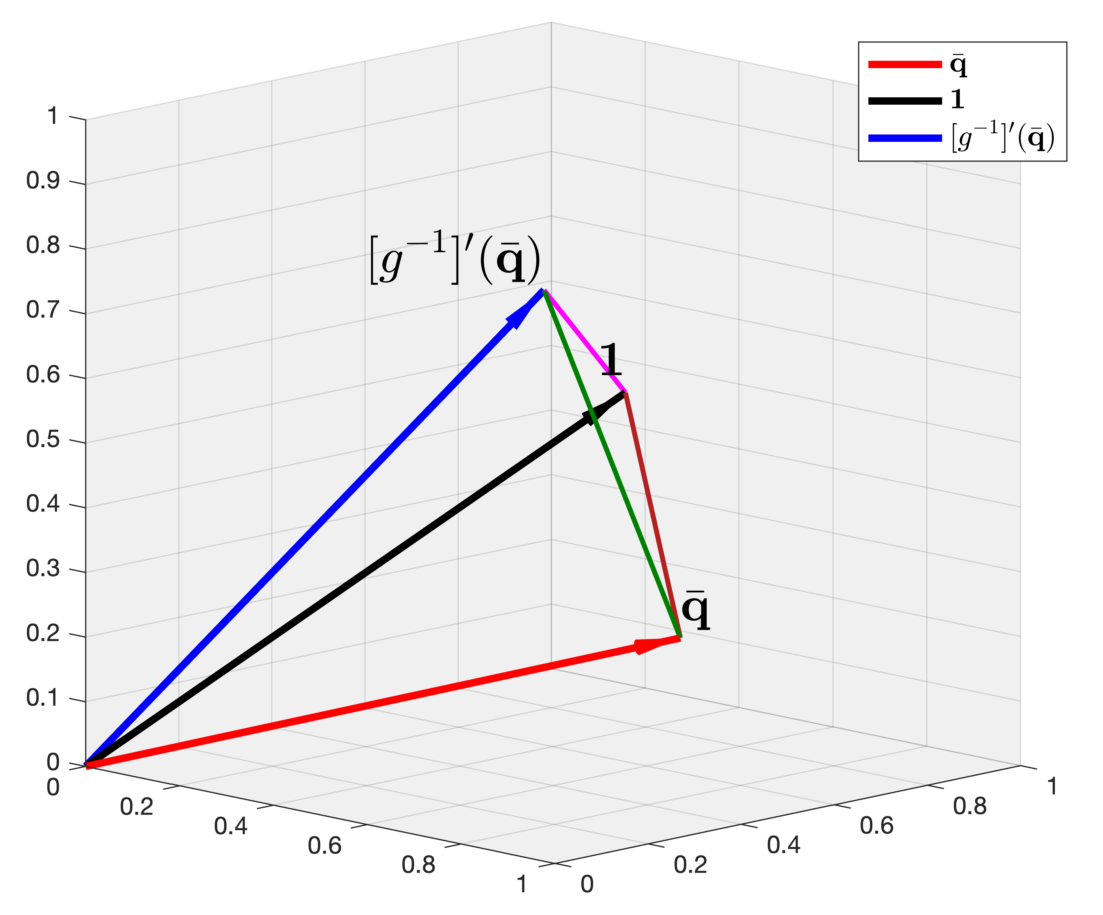
Figure 1: Relationship between the vectors $\bar{\boldsymbol{q}}$, $\left[g^{-1}\right]^{\prime}\left(\bar{\boldsymbol{q}}\right)$ and $\boldsymbol{1}$ for $\ell\left(z\right)=1/\left(1-z\right)$.

An extensive body of work implicitly characterizes the implicit bias of optimization algorithms as solutions to various convex programs [50, 28, 27, 29, 18, 19, 58, 42]. The convex program formulation typically does not admit a closed-form solution with the exception of gradient descent and the squared loss (which yields the MNI for linear models [15]). Early work here was tailored to exponential-tailed losses [50, 28], and their established equivalence to the MNI and thereby the squared loss [40, 23, 56, 55, 10] in turn heavily rely on the intermediate SVM formulation. The more recent works [42, 27, 29] study some non-exponential losses, but leave the exact nature of the implicit bias somewhat mysterious other than that the ensuing convex program no longer corresponds to the max-margin SVM. For example, [27, Figure 1] provides a simulated example for which exponential and polynomial losses induce very different directions, and [27, Proposition 12] provides an example under which the margin can be arbitrarily worse for polynomial losses. These are specialized examples of $2$-dimensional data that is linearly separable; therefore, do not apply to the high-dimensional regime of interest. The question of whether such heavy-tailed losses are actually provably worse than exponential losses is left open.

The recent papers [27, 29] provide promising avenues to understanding the nature of the implicit bias by formulating convex programs for general losses. [27] make minimal assumptions on the loss function and characterize the implicit bias as the limit of a set of solutions to convex programs with increasing $\ell_{2}$-norm (i.e. a regularization path). [57, Appendix A] show for polynomial losses that this limit can itself be written as the solution to an explicit convex program, but their proof is tailored to polynomial losses and in particular their property of positive homogeneity (and no closed-form characterization is provided). On the other hand, [29] make stronger assumptions on the loss function, but provide a clearer path to characterizing a closed-form solution for the implicit bias by understanding its mirror-descent dual as a solution to an explicit convex program (i.e. not a limit of solutions to convex programs on the regularization path). It is thus natural to attempt to obtain closed-form expressions for the “primal” implicit bias by understanding its “dual” for general losses. A second advantage with analyzing the mirror-descent dual is that we show it automatically yields the non-trivial variable substitution of the multiclass SVM dual that was made in [55], resulting in a conceptually simpler proof of SVM equivalence to MNI for the cross-entropy loss. We also show that the primal-dual analysis is applicable to more general formulations of multiclass losses [22].

Our work focuses on characterizing closed-form properties of the implicit bias in high dimensions, rather than providing non-asymptotic risk bounds. In Appendix A we contextualize our work with recent end-to-end analyses of test risk arising from various training losses.

Notation:

We use lower-case boldface (e.g. $\boldsymbol{x}$) to denote vector notation and upper-case boldface (e.g. $\boldsymbol{X}$) to denote matrix notation. We use $\left\|\cdot\right\|_{2}$ to denote the $\ell_{2}$-norm of a vector and the operator norm of a matrix. $\text{diag}\left(\boldsymbol{x}\right)$ denotes the diagonal matrix whose entries are given by the vector $\boldsymbol{x}$. For a 1-dimensional function $h(\cdot)\mathrel{\mathop{\mathchar 58\relax}}\mathbb{R}\to\mathbb{R}$, we frequently overload notation and denote its element-wise operation on a vector by $h(\boldsymbol{x})\mathrel{\mathop{\mathchar 58\relax}}=\left(h(x_{1}),\cdots,h(x_{n})\right)^{\top}$. All other appearances of the notation $h(\boldsymbol{x})\mathrel{\mathop{\mathchar 58\relax}}\mathbb{R}^{n}\to\mathbb{R}$ instead denote a function that takes a vector-valued argument. We denote first and second derivatives by ^′ and ^′′ respectively, and use $\partial$ to denote a partial derivative. We use the shorthand notation $[n]$ to denote the set of natural numbers $\{1,\ldots,n\}$.

2 Approximate Equivalences for Binary Classification

Since our results build on the primal-dual analysis presented in [29], we reproduce their assumptions on the data and loss function below.

Problem setup.

We consider a labeled dataset $\left\{\boldsymbol{x}_{i},y_{i}\right\}_{i=1}^{n}$, where $\boldsymbol{x}_{i}\in\mathbb{R}^{d}$ satisfies the normalization $\left\|\boldsymbol{x}_{i}\right\|_{2}\leq 1$ (which can be done without loss of generality) and the labels $y_{i}\in\left\{-1,1\right\}$ are binary. We denote $\boldsymbol{X}=\left(\boldsymbol{x}_{1},\cdots,\boldsymbol{x}_{n}\right)^{\top}\in\mathbb{R}^{n\times d}$ and $\boldsymbol{y}\mathrel{\mathop{\mathchar 58\relax}}=\left(y_{1},\cdots,y_{n}\right)^{\top}\in\mathbb{R}^{n}$. We focus on an unbounded, unregularized empirical risk minimization (ERM) problem with a linear classifier:

$$\underset{\boldsymbol{w}\in\mathbb{R}^{d}}{\min}\mathcal{R}\left(\boldsymbol{w}\right)\mathrel{\mathop{\mathchar 58\relax}}=\frac{1}{n}\sum_{i=1}^{n}\ell\left(-y_{i}\left\langle\boldsymbol{w},\boldsymbol{x}_{i}\right\rangle\right)=\frac{1}{n}\sum_{i=1}^{n}\ell\left(y_{i}\left\langle\boldsymbol{w},\boldsymbol{z}_{i}\right\rangle\right),$$ (1)

where we denote $\boldsymbol{z}_{i}\mathrel{\mathop{\mathchar 58\relax}}=-\boldsymbol{x}_{i}$, $\boldsymbol{Z}\mathrel{\mathop{\mathchar 58\relax}}=-\boldsymbol{X}$, and $\boldsymbol{w}\in\mathbb{R}^{d}$ is the set of parameters of the linear classifier.

Assumption 1.

The loss function $\ell(\cdot)$ satisfies:

1. $\ell$, $\ell^{\prime}$, $\ell^{\prime\prime}>0$, and $\underset{z\rightarrow-\infty}{\lim}\ell\left(z\right)=0$.

2. $z\ell^{\prime}\left(z\right)/\ell\left(z\right)$ is increasing on $(-\infty,0)$, and $\underset{z\rightarrow-\infty}{\lim}z\ell^{\prime}\left(z\right)=0$.

3. For all $b\geq 1$, there exists $c>0$ (which may depend on $b$), such that for all $a>0$, we have $\ell^{\prime}\left(\ell^{-1}\left(a\right)\right)/\ell^{\prime}\left(\ell^{-1}\left(ab\right)\right)\geq c$. Specifically, there exists a function $g\left(\cdot\right)$ such that $\underset{a\to 0}{\lim}\frac{\ell^{\prime}\left(\ell^{-1}\left(a\right)\right)}{\ell^{\prime}\left(\ell^{-1}\left(ab\right)\right)}=g\left(\frac{1}{b}\right)$, where $g\mathrel{\mathop{\mathchar 58\relax}}[0,1]\rightarrow[0,1]$ is a non-negative, strictly increasing, convex and invertible function satisfying $g\left(0\right)=0$ and $g\left(1\right)=1$.

4. Given $\boldsymbol{\xi}\in\mathbb{R}^{n}$, we define

   $$\mathcal{L}\left(\boldsymbol{\xi}\right)\mathrel{\mathop{\mathchar 58\relax}}=\sum_{i=1}^{n}\ell\left(\xi_{i}\right),\text{ and }\psi\left(\boldsymbol{\xi}\right)\mathrel{\mathop{\mathchar 58\relax}}=\ell^{-1}\left(\mathcal{L}\left(\boldsymbol{\xi}\right)\right),$$

   and consider the “generalized sum” $\psi$ to be convex and $\beta$-smooth with respect to $\ell_{\infty}$ norm.

A few comments about Assumption 1 are in order. Parts 1, 2 and 4 of the assumption are identical to the corresponding [29, Assumption 1, Parts 1, 2 and 4], and Part 3 is a strengthening of [29, Assumption 1, Part 3]. While the requirement that $\ell^{\prime}\left(\ell^{-1}\left(a\right)\right)/\ell^{\prime}\left(\ell^{-1}\left(ab\right)\right)\geq c>0$ for all $a>0,b\geq 1$ implicitly defines a function $g\left(\frac{1}{b}\right)\mathrel{\mathop{\mathchar 58\relax}}=\lim_{a\to 0}\ell^{\prime}\left(\ell^{-1}\left(a\right)\right)/\ell^{\prime}\left(\ell^{-1}\left(ab\right)\right)$, and Part 1 of Assumption 1 already ensures that $g\left(\cdot\right)$ is non-negative, strictly increasing and invertible, we additionally impose convexity on $g\left(\cdot\right)$. Figure 2 displays various examples of the form the function $g\left(\cdot\right)$ takes for specific practical loss functions. We use the convexity of $g(\cdot)$ to simplify the convex program underlying the dual implicit bias; this extra assumption is therefore central to all of our results.

The implicit bias formulation.

We use the gradient descent algorithm to solve this unregularized empirical risk minimization problem with initial weights $\boldsymbol{w}_{0}$ and the update rule: $\boldsymbol{w}_{t+1}\mathrel{\mathop{\mathchar 58\relax}}=\boldsymbol{w}_{t}-\eta_{t}\nabla\mathcal{R}\left(\boldsymbol{w}_{t}\right)$ for $t\geq 0$. We also denote, in the context of mirror-descent analysis, the “primal” $\boldsymbol{p}_{t}\mathrel{\mathop{\mathchar 58\relax}}=\text{diag}\left(\boldsymbol{y}\right)\boldsymbol{Z}\boldsymbol{w}_{t}\in\mathbb{R}^{n}$ and its corresponding “dual” $\boldsymbol{q}_{t}\mathrel{\mathop{\mathchar 58\relax}}=\nabla\psi\left(\boldsymbol{p}_{t}\right)\in\mathbb{R}^{n}$, where

$$q_{t,i}=\frac{\ell^{\prime}\left(p_{t,i}\right)}{\ell^{\prime}\left(\ell^{-1}\left(\sum_{i=1}^{n}\ell\left(p_{t,i}\right)\right)\right)}=\frac{\ell^{\prime}\left(p_{t,i}\right)}{\ell^{\prime}\left(\psi\left(\boldsymbol{p}_{t}\right)\right)}.$$ (2)

These mirror-descent primal and dual terms were defined in [29]. Next, we assume that the data can be interpolated or perfectly fitted, which corresponds to a full-rank assumption on the Gram matrix $\boldsymbol{X}\boldsymbol{X}^{\top}$. Note that this in turn implies that the dataset is linearly separable. This full-rank assumption is satisfied with high probability in the overparameterized regime $d\gg n$ for most canonical data distributions; see, e.g. [23].

Assumption 2.

We assume that $d\geq n$ and the data Gram matrix satisfies $\boldsymbol{X}\boldsymbol{X}^{\top}\succ\boldsymbol{0}$. This in turn implies that there exists $\boldsymbol{u}\in\mathbb{R}^{d}$ that $y_{i}\left\langle\boldsymbol{u},\boldsymbol{x}_{i}\right\rangle>0$ for all $i\in[n]$.

We restate the primal-dual implicit bias formulation of [29, Theorem 5] below.

Lemma 1 ([29]).

Under Assumptions 1 and 2, and provided that $\hat{\eta}_{t}\leq 1/\beta$ is nonincreasing and $\sum_{t=0}^{\infty}\hat{\eta}_{t}=\infty$, the primal and dual implicit bias $(\bar{\boldsymbol{w}},\bar{\boldsymbol{q}})$ are given by:

$$\bar{\boldsymbol{w}}\mathrel{\mathop{\mathchar 58\relax}}=\underset{t\rightarrow\infty}{\lim}\frac{\boldsymbol{w}_{t}}{\left\|\boldsymbol{w}_{t}\right\|_{2}}=\frac{-\boldsymbol{Z}^{\top}\text{diag}\left(\boldsymbol{y}\right)\bar{\boldsymbol{q}}}{\left\|-\boldsymbol{Z}^{\top}\text{diag}\left(\boldsymbol{y}\right)\bar{\boldsymbol{q}}\right\|_{2}}=\frac{\boldsymbol{X}^{\top}\text{diag}\left(\boldsymbol{y}\right)\bar{\boldsymbol{q}}}{\left\|\boldsymbol{X}^{\top}\text{diag}\left(\boldsymbol{y}\right)\bar{\boldsymbol{q}}\right\|_{2}},$$ (3)

and

$$\bar{\boldsymbol{q}}\in\underset{\psi^{*}\left(\boldsymbol{q}\right)\leq 0}{\arg\min\,}f\left(\boldsymbol{q}\right),$$ (4)

where $\psi^{*}$ denotes the convex conjugate of $\psi$, and we define $f\left(\boldsymbol{q}\right)\mathrel{\mathop{\mathchar 58\relax}}=\frac{1}{2}\left\|\boldsymbol{X}^{\top}\text{diag}\left(\boldsymbol{y}\right)\boldsymbol{q}\right\|_{2}^{2}$.

Consequently, a characterization of any solution $\bar{\boldsymbol{q}}$ to the convex program (4) defined in Lemma 1 would directly characterize the desired primal implicit bias $\bar{\boldsymbol{w}}$. Accordingly, our techniques and results largely focus on characterizing a suitable solution $\bar{\boldsymbol{q}}$ to (4).

Minimum-norm interpolation:

We are especially interested in relating the primal implicit bias $\bar{\boldsymbol{w}}$ to the minimum-norm interpolation (MNI) $\boldsymbol{w}_{\text{MNI}}\mathrel{\mathop{\mathchar 58\relax}}=\boldsymbol{X}^{\top}\left(\boldsymbol{X}\boldsymbol{X}^{\top}\right)^{-1}\boldsymbol{y}$. The MNI arises as the implicit bias of gradient descent applied to the square loss under a sufficiently small step size and initialization $\boldsymbol{w}_{0}=\boldsymbol{0}$ [15]. For example, it is easy to see that the candidate dual solution $\boldsymbol{q}\mathrel{\mathop{\mathchar 58\relax}}=\text{diag}\left(\boldsymbol{y}\right)\left(\boldsymbol{X}\boldsymbol{X}^{\top}\right)^{-1}\boldsymbol{y}$ would correspond to a primal solution proportional to $\boldsymbol{w}_{\text{MNI}}$; we will utilize this candidate solution in our equivalence results.

2.1 Main Results

The convex program defined in (4) is challenging to directly work with and analyze. This is primarily because the convex conjugate constraint $\psi^{*}\left(\boldsymbol{q}\right)$ is in general an implicitly defined function on $\boldsymbol{q}$ (with the exception of the exact exponential loss as shown in [29]), and therefore its non-positivity can be difficult to verify. To make progress, we present a simple but critical relaxation of the convex program underlying the dual implicit bias in Lemma 2 that utilizes the convex function $g\left(\cdot\right)$ defined in Assumption 1, Part 3.

Lemma 2.

Under Assumptions 1 and 2, any solution to the relaxed convex program

$$\bar{\boldsymbol{q}}\in \underset{\boldsymbol{q}\in\mathbb{R}^{n}}{\arg\min\,}\underset{f\left(\boldsymbol{q}\right)}{\underbrace{\frac{1}{2}\boldsymbol{q}^{\top}\text{diag}\left(\boldsymbol{y}\right)\boldsymbol{X}\boldsymbol{X}^{\top}\text{diag}\left(\boldsymbol{y}\right)\boldsymbol{q}}}$$ (5)

subject to $$-q_{i}<0\hskip 10.00002pt\ignorespaces\text{for all}\;i\in[n],\text{ and }\hskip 10.00002pt\ignorespaces 1-\sum_{i=1}^{n}g^{-1}\left(q_{i}\right)\leq 0.$$

is also an optimal solution to the original convex program (4).

The full proof for Lemma 2 is contained in Appendix B.1. The proof of Lemma 2 follows via a two-part argument. First, we show that the convex conjugate constraint in the convex program (4) (and in particular the implicit requirement that $\boldsymbol{q}\in\text{dom\,}\psi^{*}$) itself implies the constraints on $\boldsymbol{q}$ in (5). Next, we show that we can drop the original convex conjugate constraint and characterize the Karush-Kahn-Tucker [30] conditions of the ensuing relaxed convex program (5). In particular we show that any optimal solution to the relaxed program must satisfy $1-\sum_{i=1}^{n}g^{-1}\left(q_{i}\right)=0$, which we show in turn implies that $\boldsymbol{q}\in\text{dom\,}\psi^{*}$ and the original constraint $\psi^{*}\left(\boldsymbol{q}\right)\leq 0$ is satisfied.

2.1.1 Warm-up: Conditions for exact equivalence to MNI

Although the relaxed convex program in (5) is simpler to analyze, it still does not admit a closed-form solution in general. We begin by providing a warm-up result characterizing settings under which (5) does admit a closed-form solution, which turns out to yield the MNI primal $\boldsymbol{w}_{\text{MNI}}$.

Proposition 1.

Under Assumptions 1 and 2, the following statements hold:

1. If $\boldsymbol{y}$ is an exact eigenvector of $\boldsymbol{X}\boldsymbol{X}^{\top}$, the implicit bias $\bar{\boldsymbol{w}}$ is parallel to the MNI $\boldsymbol{w}_{\text{MNI}}$, i.e. $\frac{\bar{\boldsymbol{w}}}{\left\|\bar{\boldsymbol{w}}\right\|_{2}}=\frac{\boldsymbol{w}_{\text{MNI}}}{\left\|\boldsymbol{w}_{\text{MNI}}\right\|_{2}}$.

2. If Assumption 1, part 3 holds specifically for the identity function $g(d)=d$, the implicit bias $\bar{\boldsymbol{w}}$ is parallel to the MNI $\boldsymbol{w}_{\text{MNI}}$, i.e. $\frac{\bar{\boldsymbol{w}}}{\left\|\bar{\boldsymbol{w}}\right\|_{2}}=\frac{\boldsymbol{w}_{\text{MNI}}}{\left\|\boldsymbol{w}_{\text{MNI}}\right\|_{2}}$ iff

   $$\boldsymbol{X}\boldsymbol{X}^{\top}\succ\boldsymbol{0}\text{ and }\boldsymbol{\beta}\mathrel{\mathop{\mathchar 58\relax}}=\left(\boldsymbol{X}\boldsymbol{X}^{\top}\right)^{-1}\boldsymbol{y}\text{ satisfies }y_{i}\beta_{i}>0\text{ for all }i\in[n].$$ (6)

The full proof of Proposition 1 is provided in Appendix B.2 and works directly with the KKT conditions of the relaxed convex program (5). We make a few remarks here about this proposition. First, note that Part 2 of Proposition 1 recovers the sufficient and necessary condition for the equivalence between the SVM and the MNI, i.e. support-vector-proliferation (SVP) originally studied in [40, 23]. This makes sense as the class of loss functions for which Assumption 1, part 3 holds specifically for the identity function $g(d)=d$ corresponds to the class of exponentially-tailed losses, which are well-known to generate implicit bias that is parallel to the SVM [50]. Next, note that the condition for general losses in Part 1 (that $\boldsymbol{y}$ is an exact eigenvector of $\boldsymbol{X}\boldsymbol{X}^{\top}$) is significantly stronger than the condition in Part 2 — while $\boldsymbol{y}$ being an exact eigenvector of $\boldsymbol{X}\boldsymbol{X}^{\top}$ implies Eq. (6), the reverse implication does not hold. We show in Proposition 3 in Section 4 that the exact-eigenvector condition is in fact necessary for any loss function that does not admit the identity function $g(d)=d$. Finally, we informally remark on some sufficient conditions under which the exact-eigenvector condition would hold. One easily verifiable case is when the Gram matrix is an exact multiple of the identity, as stated below.

Corollary 1.

If $\boldsymbol{X}\boldsymbol{X}^{\top}=\alpha\boldsymbol{I}$ for some $\alpha>0$, then we have $\bar{\boldsymbol{q}}\propto\boldsymbol{1}$ and $\bar{\boldsymbol{w}}\propto\boldsymbol{w}_{\text{MNI}}$ for any loss satisfying Assumption 1.

Corollary 1 describes a scenario that will not arise in practice, as in general the Gram matrix $\boldsymbol{X}$ will be random. [41] showed that the scenario $\boldsymbol{X}\boldsymbol{X}^{\top}=\alpha\boldsymbol{I}$ can, however, arise with data that is uniformly spaced in conjunction with certain feature families. Uniformly-spaced data models also appear in some pedagogical analyses of nonparametric statistics, as they often provide a simpler analysis as compared to random data [43, 54].

2.1.2 Main result: Approximate equivalence to MNI in high dimensions

We now turn to more realistic scenarios to handle random data. In general, we only expect the Gram matrix to be close to a multiple of the identity (in the sense that the operator norm of the difference $\left\|\boldsymbol{X}\boldsymbol{X}^{\top}-\alpha\boldsymbol{I}\right\|_{2}$ is typically controlled in high dimensions). This leads to the question of whether the solution $\bar{\boldsymbol{w}}$ is now close in its direction to $\boldsymbol{w}_{\text{MNI}}$. Theorem 1 below addresses this question.

Theorem 1.

Under Assumptions 1 and 2, consider any value of $\alpha>0$ satisfying $\frac{\left\|\boldsymbol{X}\boldsymbol{X}^{\top}-\alpha\boldsymbol{I}\right\|_{2}}{\alpha}\leq\frac{1}{3}$. Then, the implicit bias $\bar{\boldsymbol{w}}$ converges in direction to $\boldsymbol{w}_{\text{MNI}}$ at the rate

$$\left\|\frac{\bar{\boldsymbol{w}}}{\left\|\bar{\boldsymbol{w}}\right\|_{2}}-\frac{\boldsymbol{w}_{\text{MNI}}}{\left\|\boldsymbol{w}_{\text{MNI}}\right\|_{2}}\right\|_{2} \leq\frac{C\left\|\boldsymbol{X}\boldsymbol{X}^{\top}\boldsymbol{y}-\alpha\boldsymbol{y}\right\|_{2}}{\alpha\left\|\boldsymbol{y}\right\|_{2}},$$ (7)

where $C$ is a universal constant that does not depend on $\alpha,\boldsymbol{X}$ or $\boldsymbol{y}$.

Theorem 1 shows that every loss function satisfying Assumption 1 yields an approximately equivalent implicit bias in high dimensions. It also recovers Corollary 1 as a special case (as in this case the RHS of Eq. (7) becomes equal to $0$).

Before discussing how to prove Theorem 1, we describe a canonical high-dimensional statistical ensemble under which it implies directional convergence of the implicit bias $\bar{\boldsymbol{w}}$ to the MNI $\boldsymbol{w}_{\text{MNI}}$.

Corollary 2.

Assume independent and identically distributed data $\{\boldsymbol{x}_{i},y_{i}\}_{i=1}^{n}$ such that each covariate $\boldsymbol{x}_{i}=\text{diag}\left(\boldsymbol{\lambda}\right)^{1/2}\boldsymbol{z}_{i}$, where $\boldsymbol{z}_{i}$ has independent entries such that each $z_{ij}$ is mean-zero, unit-variance, and sub-Gaussian with parameter $v>0$ (i.e. $\mathbb{E}[z_{ij}]=0,\mathbb{E}[z_{ij}^{2}]=1$, and $\mathbb{E}[e^{tz_{ij}}]\leq e^{vt^{2}/2}$ for all $t\in\mathbb{R}$). Also define the effective dimensions $d_{2}\mathrel{\mathop{\mathchar 58\relax}}=\frac{\left\|\boldsymbol{\lambda}\right\|_{1}^{2}}{\left\|\boldsymbol{\lambda}\right\|_{2}^{2}}$ and $d_{\infty}\mathrel{\mathop{\mathchar 58\relax}}=\frac{\left\|\boldsymbol{\lambda}\right\|_{1}}{\left\|\boldsymbol{\lambda}\right\|_{\infty}}$ and assume that $d_{2}\gg v^{2}n$ and $d_{\infty}\gg vn$. Then, Theorem 1 implies that

$$\left\|\frac{\bar{\boldsymbol{w}}}{\left\|\bar{\boldsymbol{w}}\right\|_{2}}-\frac{\boldsymbol{w}_{\text{MNI}}}{\left\|\boldsymbol{w}_{\text{MNI}}\right\|_{2}}\right\|_{2} \leq C\cdot v\cdot\max\left\{\sqrt{\frac{n}{d_{2}}},\frac{n}{d_{\infty}}\right\},$$

with probability at least $1-4e^{-cn}$, where $C,c>0$ are appropriately chosen universal constants. This implies that $\left\|\frac{\bar{\boldsymbol{w}}}{\left\|\bar{\boldsymbol{w}}\right\|_{2}}-\frac{\boldsymbol{w}_{\text{MNI}}}{\left\|\boldsymbol{w}_{\text{MNI}}\right\|_{2}}\right\|_{2}$ is vanishingly small for any high-dimensional ensemble $\{(n,d,\boldsymbol{\lambda})\}_{n\geq 1}$ satisfying $d_{2}\gg v^{2}n$ and $d_{\infty}\gg vn$.

The proof of Corollary 2 is in Appendix B.4 and applies the operator norm concentration inequality of [23, Lemma 8] (which in turn uses a volume argment from [45]). The corollary demonstrates the role of a sufficiently high-dimensional ensemble in ensuring that the implicit bias from a general convex loss eventually converges, in a directional sense, to the MNI. As a special case, consider the isotropic high-dimensional ensemble for which $\boldsymbol{\lambda}=\boldsymbol{1}$ and $v=1$. Here, we have $d_{2}=d_{\infty}=d$, and the required effective dimension conditions reduce to $d\gg n$. [23] shows that when $d_{2}\gg v^{2}n$ and $d_{\infty}\gg vn\log n$, the stronger phenomenon of SVP would occur, working from the condition in Proposition 1 Part 2.

The independent sub-Gaussian setting considered in Corollary 2 does not directly cover certain high-dimensional ensembles for which conditions for SVP have been characterized; in particular, mixture models [56, 55, 10]. We believe that results similar to Corollary 2 can also be established for these cases.

Proof sketch for Theorem 1:

Due to space limitations, we defer the full proof of Theorem 1 to Appendix B.3 and only describe the approach and main ideas here. We divide the proof in four steps. In Step 1, we begin with the relaxed convex program (5), and determine necessary characteristic equations for the solution $\bar{\boldsymbol{q}}$; in particular, we show that it is necessary for $\bar{\boldsymbol{q}}$ to solve the system of nonlinear equations $\boldsymbol{X}\boldsymbol{X}^{\top}\text{diag}\left(\boldsymbol{y}\right)\bar{\boldsymbol{q}}=\mu\text{diag}\left(\boldsymbol{y}\right)\left[g^{-1}\right]^{\prime}\left(\bar{\boldsymbol{q}}\right)$ for some $\mu>0$. In Step 2, we use the relative closeness (in an operator-norm sense) of $\boldsymbol{X}\boldsymbol{X}^{\top}$ to a multiple of $\boldsymbol{I}$ to show that the nonlinear equation above implies that the vectors $\bar{\boldsymbol{q}}$ and $\left[g^{-1}\right]^{\prime}\left(\bar{\boldsymbol{q}}\right)$ are close in a directional sense. Next, Step 3 proves a simple but non-trivial observation which, as pictured in Figure 2, states that the vector $\boldsymbol{1}$ is in between the vectors $\bar{\boldsymbol{q}}$ and $\left[g^{-1}\right]^{\prime}\left(\bar{\boldsymbol{q}}\right)$ (implying that its angle with either of the vectors is smaller than the angle between $\bar{\boldsymbol{q}}$ and $\left[g^{-1}\right]^{\prime}\left(\bar{\boldsymbol{q}}\right)$). The proof of this observation critically uses the convexity of $g(\cdot)$ which turns out to lead to an application of Chebyshev’s sum inequality [20] to complete the desired argument. Steps 1, 2 and 3 together give a rate on the directional convergence of the dual optimal solution $\bar{\boldsymbol{q}}$ to $\boldsymbol{1}$. The final Step 4 uses the primal-dual relationship in Eq. (2) to show that the primal convergence rate is identical to the dual convergence rate up to universal constant factors and is proved through a series of algebraic manipulations which repeatedly utilize the operator-norm concentration of $\boldsymbol{X}\boldsymbol{X}^{\top}$ around $\alpha\boldsymbol{I}$.

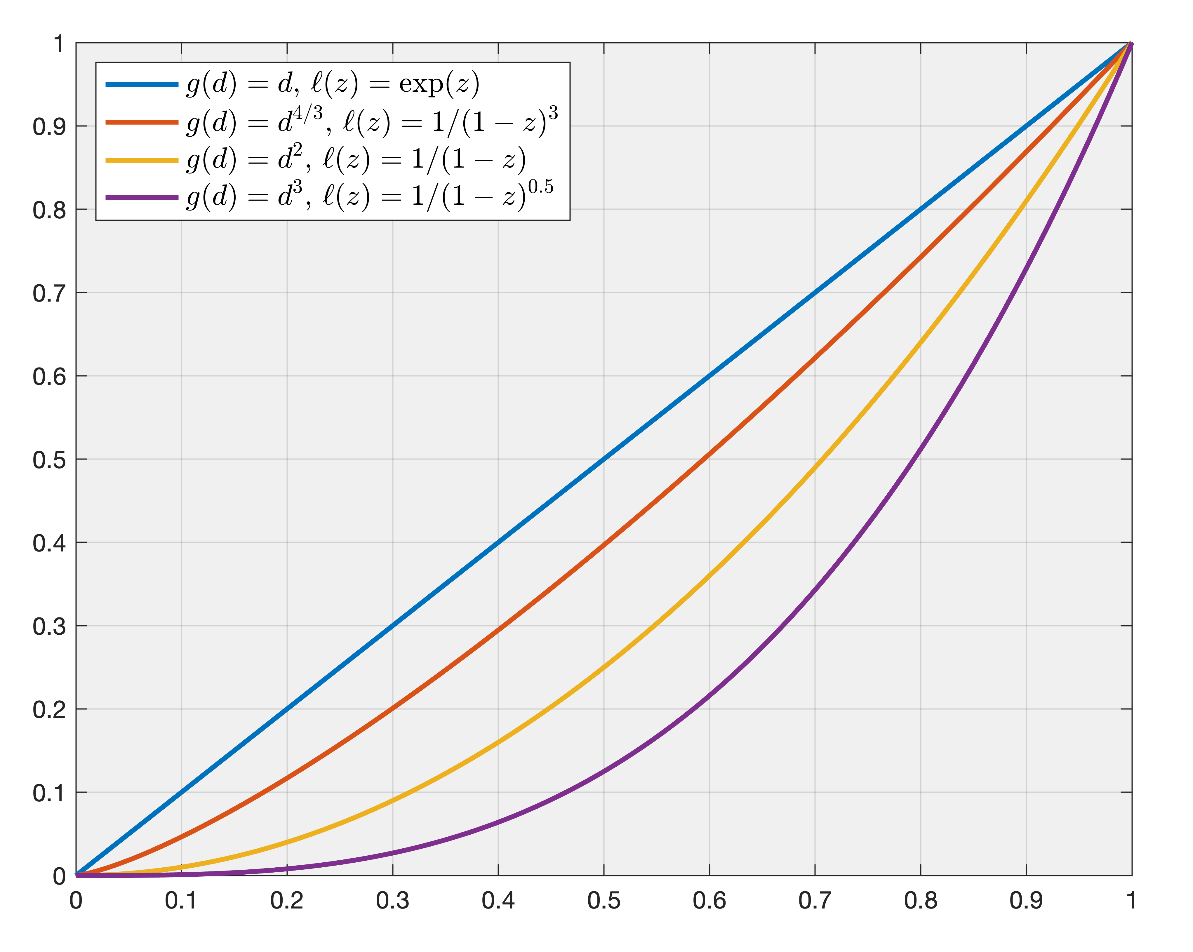
Figure 2: Plots of $g(\cdot)$ for different losses.

Loss functions satisfying Assumption 1:

We conclude this section with a brief discussion of popular loss functions that satisfy Assumption 1, and to which Proposition 1 and Theorem 1 are therefore applicable. These loss functions are also discussed in [29, Sec. 5].

Proposition 2.

Assumption 1 is satisfied by the following losses for the following choices of $g(\cdot)$:

$$\text{Exponential loss: }\ell_{\text{exp}} \mathrel{\mathop{\mathchar 58\relax}}=\exp\left(z\right),g_{\text{exp}}\left(d\right)=d$$

$$\text{Logistic loss: }\ell_{\text{log}} \mathrel{\mathop{\mathchar 58\relax}}=\ln\left(1+\exp\left(z\right)\right),g_{\text{log}}\left(d\right)=d$$

$$\text{Polynomial loss (degree $m>0$): }\ell_{\text{poly}}\left(z\right) \mathrel{\mathop{\mathchar 58\relax}}=\left\{\begin{matrix}\frac{1}{\left(1-z\right)^{m}}&,\;z\leq 0\\ \frac{1}{\left(1+z\right)^{m}}+2mz&,\;z>0\end{matrix}\right.\,,g_{\text{poly}}\left(d\right)=d^{\frac{m+1}{m}}.$$

The proof of Proposition 2 is provided in Appendix B.5 and focuses on proving the stronger condition in Assumption 1 Part 3. A plot of the function $g(\cdot)$ that underlies each loss is given in Figure 2. Note that $g(\cdot)$ that deviate more from $g(d)=d$ are heavier-tailed that the furthest pictured such function corresponds to the purple line $g(d)=d^{3}$ for the polynomial loss with degree $m=0.5$.

3 Approximate equivalences for multiclass classification

We now turn to the multiclass setting and consider a labeled dataset $\left\{\boldsymbol{x}_{i},y_{i}\right\}_{i=1}^{n}$, where $\boldsymbol{x}_{i}\in\mathbb{R}^{d}$ and $y_{i}\in[K]$. We assume there is at least one example in each class. For each class $k$, we assign a weight vector $\boldsymbol{w}_{k}\in\mathbb{R}^{d}$. We denote as shorthand $\boldsymbol{X}=\left(\boldsymbol{x}_{1},\cdots,\boldsymbol{x}_{n}\right)^{\top}\in\mathbb{R}^{n\times d}$, and an encoding of the multiclass labels $\boldsymbol{c}_{k}=\left(c_{k,1},\cdots,c_{k,n}\right)^{\top}\in\mathbb{R}^{n}$, where $c_{k,i}=\left\{\begin{matrix}\alpha&,\;k=y_{i}\\ -\beta&,\;k\neq y_{i}\end{matrix}\right.\,\forall\alpha,\beta>0$ for all $i\in[n]$ and $k\in[K]$. We assume w.l.o.g. that $\left\|\boldsymbol{x}_{i}\right\|_{2}\leq\underset{k\in[K]}{\max}c_{k,i}$. We concatenate the weight vector, data matrix and label matrix across classes as below.

$$\boldsymbol{W}=\left[\begin{matrix}\boldsymbol{w}_{1}\\ \vdots\\ \boldsymbol{w}_{k}\\ \end{matrix}\right]\in\mathbb{R}^{Kd},\;\tilde{\boldsymbol{X}}=\left[\begin{matrix}\boldsymbol{X}&\cdots&0\\ \vdots&\ddots&\vdots\\ 0&\cdots&\boldsymbol{X}\\ \end{matrix}\right]\in\mathbb{R}^{Kn\times Kd},\;\boldsymbol{C}=\left[\begin{matrix}\text{diag}\left(\boldsymbol{c}_{1}^{-1}\right)&\cdots&0\\ \vdots&\ddots&\vdots\\ 0&\cdots&\text{diag}\left(\boldsymbol{c}_{K}^{-1}\right)\\ \end{matrix}\right]\in\mathbb{R}^{Kn\times Kn}.$$

We focus on an unbounded, unregularized ERM problem with a linear classifier:

$$\underset{\boldsymbol{W}\in\mathbb{R}^{Kd}}{\min}\mathcal{R}\left(\boldsymbol{W}\right)\mathrel{\mathop{\mathchar 58\relax}}=\frac{1}{n}\sum_{i=1}^{n}\mathfrak{L}\left(-\left\{c_{k,i}^{-1}\left\langle\boldsymbol{w}_{k},\boldsymbol{x}_{i}\right\rangle\right\}_{k=1}^{K}\right)=\frac{1}{n}\sum_{i=1}^{n}\mathfrak{L}\left(\left\{c_{k,i}^{-1}\left\langle\boldsymbol{w}_{k},\boldsymbol{z}_{i}\right\rangle\right\}_{k=1}^{K}\right),$$ (8)

where we denote $\boldsymbol{z}_{i}\mathrel{\mathop{\mathchar 58\relax}}=-\boldsymbol{x}_{i}$, and therefore $\boldsymbol{Z}\mathrel{\mathop{\mathchar 58\relax}}=-\boldsymbol{X}\in\mathbb{R}^{n\times d}$ and $\tilde{\boldsymbol{Z}}=-\tilde{\boldsymbol{X}}\in\mathbb{R}^{Kn\times Kd}$. We assume that the loss function $\mathfrak{L}$ either satisfies the following Assumption  3 or Assumption 4.

Assumption 3.

The loss function $\mathfrak{L}$ proposed for a multiclass extension of AdaBoost [22] satisfies

$$\mathfrak{L}\left(\left\{c_{k,i}^{-1}\left\langle\boldsymbol{w}_{k},\boldsymbol{z}_{i}\right\rangle\right\}_{k=1}^{K}\right)=\ell\left(-\sum_{k=1}^{K}c_{k,i}^{-1}\left\langle\boldsymbol{w}_{k},\boldsymbol{x}_{i}\right\rangle\right)=\ell\left(\sum_{k=1}^{K}c_{k,i}^{-1}\left\langle\boldsymbol{w}_{k},\boldsymbol{z}_{i}\right\rangle\right),$$

where $\ell$ satisfies Assumption 1 Parts 1, 2 and 3. Additionally, given $\boldsymbol{\xi}_{k}\in\mathbb{R}^{n}$ and $\boldsymbol{\Xi}=\left(\boldsymbol{\xi}_{1}^{\top},\cdots,\boldsymbol{\xi}_{K}^{\top}\right)^{\top}\in\mathbb{R}^{Kn}$, we define $\mathcal{L}\left(\boldsymbol{\Xi}\right)\mathrel{\mathop{\mathchar 58\relax}}=\sum_{i=1}^{n}\mathfrak{L}\left(\left\{\xi_{k,i}\right\}_{k=1}^{K}\right)=\sum_{i=1}^{n}\ell\left(\sum_{k=1}^{K}\xi_{k,i}\right)$ and $\psi\left(\boldsymbol{\Xi}\right)\mathrel{\mathop{\mathchar 58\relax}}=\ell^{-1}\left(\mathcal{L}\left(\boldsymbol{\Xi}\right)\right)$, where $\psi$ is jointly convex and $\beta$-smooth with respect to $\ell_{\infty}$ norm.

Assumption 4 (Cross-entropy loss).

The loss function $\mathfrak{L}$ satisfies

$$\mathfrak{L}\left(\left\{c_{k,i}^{-1}\left\langle\boldsymbol{w}_{k},\boldsymbol{z}_{i}\right\rangle\right\}_{k=1}^{K}\right) =-\ln\left(\frac{\exp\left(\left\langle\boldsymbol{w}_{y_{i}},\boldsymbol{x}_{i}\right\rangle\right)}{\sum_{k=1}^{K}\exp\left(\left\langle\boldsymbol{w}_{k},\boldsymbol{x}_{i}\right\rangle\right)}\right)$$

$$=\ln\left(1+\sum_{k\neq y_{i}}^{K}\exp\left(c_{y_{i},i}\left(c_{y_{i},i}^{-1}\left\langle\boldsymbol{w}_{y_{i}},\boldsymbol{z}_{i}\right\rangle\right)-c_{k,i}\left(c_{k,i}^{-1}\left\langle\boldsymbol{w}_{k_{i}},\boldsymbol{z}_{i}\right\rangle\right)\right)\right).$$

Given $\boldsymbol{\xi}_{k}\in\mathbb{R}^{n}$, $\boldsymbol{\Xi}=\left(\boldsymbol{\xi}_{1}^{\top},\cdots,\boldsymbol{\xi}_{K}^{\top}\right)^{\top}\in\mathbb{R}^{Kn}$, and $\ell\left(z\right)=\ln\left(1+\exp\left(z\right)\right)$, we define

$$\mathcal{L}\left(\boldsymbol{\Xi}\right)\mathrel{\mathop{\mathchar 58\relax}} =\sum_{i=1}^{n}\mathfrak{L}\left(\left\{\xi_{k,i}\right\}_{k=1}^{K}\right)=\sum_{i=1}^{n}\ln\left(1+\sum_{k\neq y_{i}}^{K}\exp\left(c_{y_{i},i}\xi_{y_{i},i}-c_{k,i}\xi_{k,i}\right)\right)$$

$$\text{and}\;\;\psi\left(\boldsymbol{\Xi}\right)\mathrel{\mathop{\mathchar 58\relax}} =\ell^{-1}\left(\mathcal{L}\left(\boldsymbol{\Xi}\right)\right),$$

where $\psi$ is individually convex with respect to each $\boldsymbol{\xi}_{k}$, and $\beta$-smooth with respect to $\ell_{\infty}$ norm.

The cross-entropy loss (Assumption 4) turns out not to fit directly in the framework of Assumption 3 and we treat it separately. For loss functions under Assumption 3 we use the “equal assignment” encoding $\alpha=\beta=1$; for the cross-entropy loss we use the “simplex representation” [34, 55] $\alpha=\frac{K-1}{K}$ and $\beta=\frac{1}{K}$. In Appendix D.3 we show that the properties of convexity and $\beta$-smoothness of $\psi$ carry over to the multiclass case and also hold for the cross-entropy loss; interestingly, for the latter we can only prove individual convexity.

3.1 Main results

First, we extend the primal-dual framework from [29] to the multiclass case. We again use gradient descent to solve this unregularized ERM problem with initialization $\boldsymbol{W}_{0}$ and update rule: $\boldsymbol{W}_{t+1}\mathrel{\mathop{\mathchar 58\relax}}=\boldsymbol{W}_{t}-\eta_{t}\nabla\mathcal{R}\left(\boldsymbol{W}_{t}\right)$ for $t\geq 0$. We denote, in the context of mirror-descent analysis, the ”primal” $\boldsymbol{P}_{t}\mathrel{\mathop{\mathchar 58\relax}}=\boldsymbol{C}\tilde{\boldsymbol{Z}}\boldsymbol{W}_{t}=\left(\boldsymbol{p}_{1,t}^{\top},\cdots,\boldsymbol{p}_{K,t}^{\top}\right)^{\top}\in\mathbb{R}^{Kn}$, and its corresponding ”dual” $\boldsymbol{Q}_{t}\mathrel{\mathop{\mathchar 58\relax}}=\nabla\psi\left(\boldsymbol{P}_{t}\right)=\left(\boldsymbol{q}_{1,t}^{\top},\cdots,\boldsymbol{q}_{K,t}^{\top}\right)^{\top}\in\mathbb{R}^{Kn}$, where $\boldsymbol{p}_{k,t}=\text{diag}\left(\boldsymbol{c}_{k}^{-1}\right)\boldsymbol{Z}\boldsymbol{w}_{k,t}\in\mathbb{R}^{n}$ and $\boldsymbol{q}_{k,t}=\nabla_{\boldsymbol{p}_{k,t}}\psi\left(\boldsymbol{P}_{t}\right)\in\mathbb{R}^{n}$ for all $k\in[K]$ and $t\geq 0$. Again, we assume that the data can be interpolated, which implies that the dataset is one-vs-all separable.

Assumption 5.

We assume that $d\geq n$ and the data Gram matrix satisfies $\boldsymbol{X}\boldsymbol{X}^{\top}\succ\boldsymbol{0}$. This in turn implies that there exists $\boldsymbol{u}_{k}\in\mathbb{R}^{d}$ for all $k\in[K]$ such that $\left\langle\boldsymbol{u}_{k},\boldsymbol{x}_{i}\right\rangle\left\{\begin{matrix}\geq 1&,\;k=y_{i}\\ \leq-1&,\;k\neq y_{i}\end{matrix}\right.\,$, for all $i\in[n]$.

This concatenated representation together with Assumptions 3, 4 and 5 ensure that the setup is identical to that of [29]. Therefore, we can directly apply their primal-dual result, which we restate below in our notation specific to the multiclass setting.

Lemma 3.

Under Assumption 3 or 4 and 5, when all $t$ with $\psi\left(\boldsymbol{C}\tilde{\boldsymbol{Z}}\boldsymbol{W}_{t}\right)\leq 0$, and iteration of gradient descent goes to infinity with $\hat{\eta}_{t}=\eta_{t}\ell^{\prime}\left(\psi\left(\boldsymbol{C}\tilde{\boldsymbol{Z}}\boldsymbol{W}_{t}\right)\right)/n\leq 1/\beta$ is nonincreasing and $\sum_{t=0}^{\infty}\hat{\eta}_{t}=\infty$, we have the implicit bias $\bar{\boldsymbol{W}}\mathrel{\mathop{\mathchar 58\relax}}=\underset{t\rightarrow\infty}{\lim}\frac{\boldsymbol{W}_{t}}{\left\|\boldsymbol{W}_{t}\right\|_{2}}=\frac{\tilde{\boldsymbol{X}}^{\top}\boldsymbol{C}\bar{\boldsymbol{Q}}}{\left\|\tilde{\boldsymbol{X}}^{\top}\boldsymbol{C}\bar{\boldsymbol{Q}}\right\|_{2}}$, where

$$\bar{\boldsymbol{Q}}\in\underset{\psi^{*}\left(\boldsymbol{Q}\right)\leq 0}{\arg\min\,}F\left(\boldsymbol{Q}\right),\text{ and }F\left(\boldsymbol{Q}\right)\mathrel{\mathop{\mathchar 58\relax}}=\frac{1}{2}\left\|\tilde{\boldsymbol{X}}^{\top}\boldsymbol{C}\boldsymbol{Q}\right\|_{2}^{2}$$ (9)

We provide the details of this proof, which is mostly an extension of [29], in Appendix C. One subtlety is that we were only able to establish individual convexity in $\psi$ for the cross-entropy loss. Lemma 13 shows that this is sufficient to recover Lemma 3, and joint convexity is only required to prove the tightness of the convergence rates in [29].

We now present the main results of this section, which are equivalences with MNI for losses satisfying Assumption 3 or 4 analogous to the binary case.

Theorem 2.

Under Assumptions 3 and 5, consider any value of $\alpha>0$ satisfying $\frac{\left\|\boldsymbol{X}\boldsymbol{X}^{\top}-\alpha\boldsymbol{I}\right\|_{2}}{\alpha}\leq\frac{1}{3}$. Then, the implicit biases $\bar{\boldsymbol{w}}_{k}$ converges in direction to $\boldsymbol{w}_{\text{MNI},k}$ at the rate:

$$\left\|\frac{\bar{\boldsymbol{w}}_{k}}{\left\|\bar{\boldsymbol{w}}_{k}\right\|_{2}}-\frac{\boldsymbol{w}_{\text{MNI},k}}{\left\|\boldsymbol{w}_{\text{MNI},k}\right\|_{2}}\right\|_{2} \leq\frac{C\left\|\boldsymbol{X}\boldsymbol{X}^{\top}\boldsymbol{c}_{k}-\alpha\boldsymbol{c}_{k}\right\|_{2}}{\alpha\left\|\boldsymbol{c}_{k}\right\|_{2}},\qquad$$ (10)

where $C$ is a universal constants that do not depend on $\alpha$, $\boldsymbol{X}$ or $\boldsymbol{c}_{k}$.

Theorem 3.

Under Assumption 4 and 5, the implicit bias parallels to simplex version MNI iff $\boldsymbol{X}\boldsymbol{X}^{\top}\succ\boldsymbol{0}$ and $\boldsymbol{\beta}_{k}\mathrel{\mathop{\mathchar 58\relax}}=\left(\boldsymbol{X}\boldsymbol{X}^{\top}\right)^{-1}\boldsymbol{c}_{k}$ satisfies $c_{k,i}\beta_{k,i}>0$ for all $i\in[n]$ and $k\in[K]$.

The detailed proofs of these results are in Appendix D.1 and D.2. The proof of Theorem 2 is a simple generalization of Theorem 1. Theorem 3 recovers the exact equivalence condition of [55]. Interestingly, the convex program on $\bar{\boldsymbol{q}}_{k}$ for all $k\in[K]$ that are formulated in the proof of Theorem 3 already contains the novel equality constraints that [55] were only able to obtain after applying a non-trivial transformation to the multiclass SVM dual variables. This suggests that the mirror-descent dual is the more natural dual to analyze in the multiclass case.

4 A converse result

We now show that the condition for exact equivalence in Proposition 1 is necessary. For conciseness we consider binary labels, but these proofs can easily be extended to the multiclass case.

Proposition 3.

Consider any loss function that satisfies Assumption 1 with a strictly convex function $g(d)\neq d$. Define $h\left(d\right)\mathrel{\mathop{\mathchar 58\relax}}=\left[g^{-1}\right]^{\prime}\left(d\right)$ and $f(d)\mathrel{\mathop{\mathchar 58\relax}}=\frac{h\left(d\right)}{d}$. Then, the following statements are true about the optimal solution $\bar{\boldsymbol{q}}$ to the dual convex program (4):

1. If $\boldsymbol{y}$ is not an exact eigenvector of $\boldsymbol{X}\boldsymbol{X}^{\top}$, then at least two of the entries in $\bar{\boldsymbol{q}}$ need to be distinct, i.e. $\bar{\boldsymbol{q}}$ cannot be parallel to $\boldsymbol{1}$; therefore, $\bar{\boldsymbol{w}}$ is not parallel to $\boldsymbol{w}_{\text{MNI}}$.

2. If $\boldsymbol{X}\boldsymbol{X}^{\top}=\boldsymbol{D}=\text{diag}\left(\boldsymbol{d}\right)$, the primal solution $\bar{\boldsymbol{w}}$ interpolates the adjusted labels $\tilde{y}_{i}=y_{i}d_{i}\cdot f^{-1}\left(\frac{d_{i}}{\mu}\right)$, where $\mu>0$ is any solution to the equation $\sum_{i=1}^{n}g^{-1}\left(f^{-1}\left(\frac{d_{i}}{\mu}\right)\right)=1$.

Proposition 3 is proved in Appendix E and also utilizes the relaxed convex program of Lemma 2. The proposition shows that the condition for exact equivalence in Eq. (6) only applies to the implicit bias of exponentially-tailed losses, which satisfy Assumption 1 with the identity mapping $g(d)=d$. Moreover, Part 1 of Proposition 1 is a sufficient and necessary condition for exact equivalence for any non-exponential loss with a non-identity mapping $g(d)\neq d$. Part 2 of Proposition 3 provides explicit counterexamples in the form of Gram matrices $\boldsymbol{X}\boldsymbol{X}^{\top}=\boldsymbol{D}$ that can easily be verified to satisfy the SVM equivalence condition $y_{i}(\boldsymbol{X}\boldsymbol{X}^{\top})^{-1}\boldsymbol{y}\succ 0$, yet, induce a very different solution from the MNI that interpolates labels adjusted differently per training example. To drive home this point, we use Proposition 3 to characterize the impact of the importance weighting procedure with polynomial losses. This procedure, parameterized by a subset of underrepresented examples $S\subset[n]$ and weight $Q>1$ and applied with a loss function $\ell(\cdot)$, minimizes the weighted risk $\mathcal{R}\left(\boldsymbol{w};(Q,S)\right)\mathrel{\mathop{\mathchar 58\relax}}=\frac{1}{n}\sum_{i=1}^{n}Q^{\mathbb{I}[i\in S]}\cdot\ell\left(-y_{i}\left\langle\boldsymbol{w},\boldsymbol{x}_{i}\right\rangle\right)$. Recently, [57] proposed applying this procedure with polynomial losses to address OOD generalization.

Corollary 3.

Consider the idealized data matrix $\boldsymbol{X}\boldsymbol{X}^{\top}=\alpha\boldsymbol{I}$ for some $\alpha>0$, as in Corollary 1. Then, importance weighting with a polynomial loss of degree $m$ leads to implicit bias $\bar{\boldsymbol{w}}$ that interpolates per-example-adjusted labels $\tilde{y_{i}}\propto Q^{\frac{1}{m+2}\cdot\mathbb{I}[i\in S]}y_{i}$.

Corollary 3 is proved in Appendix E.2 and implies that importance weighting with polynomial losses will interpolate labels that are larger in magnitude on minority points. As shown in [31, 7], this type of cost-sensitive interpolation is provably beneficial for OOD generalization. Since $Q>1$, heavier-tailed polynomial losses (corresponding to smaller values of $m$) lead to a stronger importance-weighting effect. One can compare this interpolation to that induced by the vector-scaling (VS-loss) [59, 31], defined as a per-example loss function $\ell_{\text{vs}}\left(z_{i};(Q,S)\right)\mathrel{\mathop{\mathchar 58\relax}}=\ln\left(1+\exp\left(Q^{\mathbb{I}[i\in S]}z_{i}\right)\right)$. [7] shows that in our high-dimensional regime, this will lead to cost-sensitive interpolation of the adjusted labels $\tilde{y}_{i}\propto Q^{\mathbb{I}[i\in S]}y_{i}$, which is in fact a stronger interpolation effect.

5 Discussion

Our results show that once we move away from the exponentially-tailed family of losses, general losses exhibit a variety of influence on the eventual solution. We believe that these results show the potential of the primal-dual framework to study closed-form properties of the implicit bias. It would be interesting to provide similar closed-form characterizations for the implicit bias of other optimization algorithms and/or for nonlinear models. Specific to linear models and gradient descent, there are still many open questions. Based on converse results in [23, 1] for exponential losses, the effective overparameterization conditions in Corollary 2 appear necessary for asymptotic directional convergence of the implicit bias to MNI. However, whether Theorem 1 provides the optimal rate of convergence is unclear. Also, of interest is whether it is possible to obtain results similar to Propositions 1 and Theorem 1 under minimal assumptions on losses such as in [27, 4]. Finally, we are interested in using these closed-form characterizations to obtain tight non-asymptotic bounds on the test risk.

Appendix A Expanded related work

In this section we provide broader context for understanding the impact of loss function on downstream generalization, both in the classical low-dimensional regime and the modern high-dimensional regime.

Classical perspectives on loss function design:

The classical perspective on loss function design, pioneered by the papers [4, 61, 35, 51] advocates for designing continuous surrogates to the discontinuous 0-1 test risk such that a bound on the 0-1 test risk can be easily obtained by inverting a bound on the surrogate test risk. In an indirect sense, this classical perspective suggests a type of equivalence in surrogate loss functions in terms of ensuing generalization bounds. However, principally because of the reliance on empirical-process-theory (to relate in turn the surrogate test risk to the surrogate training loss), this reasoning can frequently break down in high-dimensional settings, particularly when perfectly fitting, or interpolating models are considered. This is because infinitely many models interpolate the training data, but each of them suffers a different test risk that is fundamentally unrelated to the training loss. On the other hand, while the relations between test risks (e.g. [4, Theorems 1 and 3]) remain universally applicable, they also suffer from some shortcomings in high-dimensional settings — in particular, they are only powerful enough to provide faster statistical rates for classification tasks as compared to parameter recovery [2], rather than full separations in asymptotic consistency (many classic examples of such separations are considered in [14], but such separations were also shown more recently in the overparameterized regime in [40]).

Generalization analysis of interpolating predictors in high dimensions:

A comprehensive theory for overparameterized models arising from training with the squared loss (i.e. the MNI) was provided in work beginning with the papers that analyzed the test regression risk [5, 8, 21, 33, 41]. This theory critically utilizes the closed-form expression for the MNI. Sharply analyzing the classification risk poses distinct challenges, the most daunting of which is the lack of a closed-form expression for the solution arising from any other convex loss function used for classification. To tackle this challenge for the special case of exponential losses, [40] introduced a two-step recipe. First, they related the implicit bias of exponential losses (i.e. the SVM) to the MNI — in fact, by showing an exact equivalence result (which was since improved on by [23]). Second, they sharply analyzed the classification test risk of the MNI and showed that it can achieve classification-consistency even when a corresponding regression task would not be consistent. It is worth noting that this type of consistency result cannot be easily recovered through any generalization bound that relies on empirical-process-theory, including margin-based data-dependent generalization bounds (as described in [40, Section 6]). This recipe was since applied to binary and multiclass Gaussian and sub-Gaussian mixture models to identify new high-dimensional regimes in which classification-consistency is possible [56, 10, 55, 52]. To be able to apply this recipe to more general losses, corresponding equivalences would need to be established between general losses and the MNI, which is the focus of this paper.

Other than the approach described above, two other families of techniques are prevalent in the recent literature. The first applies to proportionally high-dimensional regimes (where $d\propto n$) and directly characterizes the limiting test risk as $(d,n)\to\infty$ as the solution to a system of nonlinear equations, beginning with the efforts [24, 53, 36, 48, 13, 39]. None of our results for general losses have direct implications for this proportional regime, except under the idealized assumption $\boldsymbol{X}\boldsymbol{X}^{\top}=\alpha\boldsymbol{I}$ made in Corollaries 1 and 3. These works have exclusively focused on exponentially-tailed losses; extending these techniques to general losses is a separate open question of interest that we do not address. However, we believe the relaxed convex program proposed in Lemma 2 might be of independent interest, particularly for the subset of approaches above that utilize Gordon’s comparison theorems as the key technique.

The second technique was proposed by [11] for directly analyzing the generalization error of the implicit bias of exponential losses on a sub-Gaussian mixture model. The key technical innovation is to prove a “loss ratio” bound: under sufficiently overparameterized settings, [11] show that the training losses of any two examples are within a constant factor of each other throughout the optimization path of gradient descent. This proof technique is quite generally applicable and was since used for polynomial losses [57], deep linear networks [12] and certain 2-layer neural networks on high-dimensional data [16]. However, the loss-ratio bound often requires a much larger data dimension $d\gg n^{2}$ to hold as compared to the MNI-equivalence approach to analyzing the SVM, as shown explicitly in [56]. It is not clear whether this dimension requirement is tight even in the worst case. A natural question of interest is whether a loss-ratio bound implies exact or approximate equivalence of solutions or vice-versa. [7] showed recently that a loss-ratio bound can imply exact equivalence to the MNI in the case of exponential losses, but this a research direction that is otherwise largely unexplored.

Appendix B Proofs of all binary results

In this section, we include all of the detailed proofs for our analysis for the binary case.

B.1 Proof of Lemma 2

In this section we prove Lemma 2. Note that the requirement that $\boldsymbol{q}\in\text{dom\,}\psi^{*}$ is implicit in the constraint $\psi^{*}\left(\boldsymbol{q}\right)\leq 0$. We utilize the following lemma to analyze the domain of $\psi^{*}\left(\boldsymbol{q}\right)$ and identify some necessary and sufficient conditions of $\bar{\boldsymbol{q}}\mathrel{\mathop{\mathchar 58\relax}}=\lim_{t\to\infty}\boldsymbol{q}_{t}\in\text{dom\,}\psi^{*}$ in particular.

Lemma 4.

Under Assumption 1, for any $\boldsymbol{q}=\left(q_{1},\cdots,q_{n}\right)^{\top}\in\text{dom\,}\psi^{*}$, we have $\boldsymbol{q}=\nabla\psi\left(\boldsymbol{p}^{*}\right)$, where $q_{i}=\frac{\ell^{\prime}\left(\ell^{-1}\left(\ell\left(p^{*}_{i}\right)\right)\right)}{\ell^{\prime}\left(\ell^{-1}\left(\sum_{i=1}^{n}\ell\left(p^{*}_{i}\right)\right)\right)}$ and $0<q_{i}\leq 1$, for some $\boldsymbol{p}^{*}=\left(p^{*}_{1},\cdots,p^{*}_{n}\right)^{\top}\in\mathbb{R}^{n}$ for all $i\in[n]$. It is additionally necessary and sufficient for $\bar{\boldsymbol{q}}\mathrel{\mathop{\mathchar 58\relax}}=\lim_{t\to\infty}\boldsymbol{q}_{t}$ to satisfy $\sum_{i=1}^{n}g^{-1}(\bar{q}_{i})=1$ to be in the domain of $\psi^{*}$.

Proof.

For any $\boldsymbol{q}=\left(q_{1},\cdots,q_{n}\right)^{\top}\in\text{dom\,}\psi^{*}$, we have $\psi^{*}\left(\boldsymbol{q}\right)=\underset{\boldsymbol{p}\in\mathbb{R}^{n}}{\sup}\left\langle\boldsymbol{p},\boldsymbol{q}\right\rangle-\psi\left(\boldsymbol{p}\right)=\left\langle\boldsymbol{p}^{*},\boldsymbol{q}\right\rangle-\psi\left(\boldsymbol{p}^{*}\right)$, where $\boldsymbol{q}=\nabla\psi\left(\boldsymbol{p}^{*}\right)$ for some $\boldsymbol{p}^{*}\in\mathbb{R}^{n}$. Therefore, we have

$$q_{i}=\frac{\ell^{\prime}\left(p^{*}_{i}\right)}{\ell^{\prime}\left(\ell^{-1}\left(\sum_{i=1}^{n}\ell\left(p^{*}_{i}\right)\right)\right)}=\frac{\ell^{\prime}\left(\ell^{-1}\left(\ell\left(p^{*}_{i}\right)\right)\right)}{\ell^{\prime}\left(\ell^{-1}\left(\sum_{i=1}^{n}\ell\left(p^{*}_{i}\right)\right)\right)}>0\text{ for all }i\in[n].$$

Moreover, we know that $\ell\left(p_{i}\right)\leq\sum_{i=1}^{n}\ell\left(p_{i}\right)$ for all $i\in[n]$. Since Assumption 1 Part 1 also requires $\ell^{\prime}$, $\ell^{\prime\prime}>0$, we have that $\ell^{-1}$ and $\ell^{\prime}$ are both non-decreasing functions, and so $\ell^{\prime}\left(\ell^{-1}\left(\cdot\right)\right)$ is a non-decreasing function as well. This implies that $q_{i}=\frac{\ell^{\prime}\left(\ell^{-1}\left(\ell\left(p_{i}\right)\right)\right)}{\ell^{\prime}\left(\ell^{-1}\left(\sum_{i=1}^{n}\ell\left(p_{i}\right)\right)\right)}\leq 1$ for all $i\in[n]$.

We now prove the additional specific property on $\bar{\boldsymbol{q}}$, first proving the necessity condition. Recall the expression from Eq. (2) and note, from [29][Theorems 1] primal convergence that $\lim_{t\to\infty}\ell(p_{t,i})=0$ for all $i\in[n]$. Therefore, defining $\alpha_{i}\mathrel{\mathop{\mathchar 58\relax}}=\lim_{t\to\infty}\frac{\ell(p_{t,i})}{\sum_{i=1}^{n}\ell(p_{t,i})}\in[0,1]$, we have

$$\bar{q}_{i}\mathrel{\mathop{\mathchar 58\relax}}=\lim_{t\to\infty}q_{t,i} =\lim_{t\to\infty}\frac{\ell^{\prime}\left(\ell^{-1}\left(\ell\left(p_{t,i}\right)\right)\right)}{\ell^{\prime}\left(\ell^{-1}\left(\sum_{i=1}^{n}\ell\left(p_{t,i}\right)\right)\right)}$$

$$=g\left(\alpha_{i}\right),$$

where the last equality follows by Assumption 1, Part 3. By definition, we have $\sum_{i=1}^{n}\alpha_{i}=1$. Consequently, we get $\sum_{i=1}^{n}\alpha_{i}=\sum_{i=1}^{n}g^{-1}(\bar{q}_{i})=1$. To prove sufficiency, consider any $\bar{\boldsymbol{q}}$ satisfying $\sum_{i=1}^{n}g^{-1}(\bar{q}_{i})=1$. We will now construct a corresponding sequence $\{\boldsymbol{p}_{t}\}_{t\geq 1}$ that yields $\bar{\boldsymbol{q}}=\lim_{t\to\infty}\nabla\psi\left(\boldsymbol{p}_{t}\right)$ such that $\lim_{t\to\infty}\ell(p_{t,i})=0$. Define $\alpha_{i}=g^{-1}(\bar{q}_{i})\in[0,1]$, and note that by definition $\sum_{i=1}^{n}\alpha_{i}=1$. Then, we can define $\ell(p_{t,i})=f_{t}\alpha_{i}$ for any fixed convergence sequence $\{f_{t}\}_{t\geq 1}$ such that $\lim_{t\to\infty}f_{t}=0$, and thereby define $p_{t,i}=\ell^{-1}(f_{t}\alpha_{i})$. It is easy to verify that $\lim_{t\to\infty}\ell(p_{t,i})=\lim_{t\to\infty}f_{t}\alpha_{i}=0$, and that $\bar{\boldsymbol{q}}=\lim_{t\to\infty}\nabla\psi(\boldsymbol{p}_{t})$ for this choice of $\boldsymbol{p}_{t}$. This completes the sufficiency part, and therefore the proof of this lemma. ∎

Next, we introduce Lemma 5 that shows that $\sum_{i=1}^{n}q_{i}\leq 1$ implies the feasibility of the convex conjugacy feasibility constraint, i.e. $\psi^{*}\left(\boldsymbol{q}\right)\leq 0$.

Lemma 5.

Any $\boldsymbol{q}\in\mathbb{R}^{n}\in\text{dom\,}\psi^{*}$ that satisfies $\sum_{i=1}^{n}q_{i}\leq 1$ also satisfies the convex conjugacy feasibility constraint $\psi^{*}\left(\boldsymbol{q}\right)\leq 0$.

Proof.

Just as in the proof of Lemma 4, note that for any $\boldsymbol{q}=\left(q_{1},\cdots,q_{n}\right)^{\top}\in\text{dom\,}\psi^{*}$, we have for all $i\in[n]$, $q_{i}=\frac{\ell^{\prime}\left(\ell^{-1}\left(\ell\left(p^{*}_{i}\right)\right)\right)}{\ell^{\prime}\left(\ell^{-1}\left(\sum_{i=1}^{n}\ell\left(p^{*}_{i}\right)\right)\right)}=\frac{\ell^{\prime}\left(p^{*}_{i}\right)}{\ell^{\prime}\left(\psi\left(\boldsymbol{p}^{*}\right)\right)}$, and $0<q_{i}\leq 1$ for some $\boldsymbol{p}^{*}=\left(p^{*}_{1},\cdots,p^{*}_{n}\right)^{\top}\in\mathbb{R}^{n}$. Multiplying both sides of the equation by $\ell^{\prime}(\psi(\boldsymbol{p}^{*}))$ and noting by Assumption 1 Part 1 that $\ell^{\prime}$ is strictly increasing, we get the implicit equation $p^{*}_{i}=\left[\ell^{\prime}\right]^{-1}\left(q_{i}\ell^{\prime}\left(\psi\left(\boldsymbol{p}^{*}\right)\right)\right)$ for all $i\in[n]$. Recall from [29, Lemma 6] that we already have $\psi^{*}\left(\boldsymbol{q}\right)\leq 0$ if $\psi\left(\boldsymbol{p}^{*}\right)\leq 0$. Therefore, we only consider the case for which $\psi\left(\boldsymbol{p}^{*}\right)>0$. We get

$$\psi^{*}\left(\boldsymbol{q}\right)=\sum_{i=1}^{n}p^{*}_{i}q_{i}-\psi\left(\boldsymbol{p}^{*}\right) =\sum_{i=1}^{n}\left[\ell^{\prime}\right]^{-1}\left(q_{i}\ell^{\prime}\left(\psi\left(\boldsymbol{p}^{*}\right)\right)\right)q_{i}-\psi\left(\boldsymbol{p}^{*}\right)$$

$$\leq\sum_{i=1}^{n}\left[\ell^{\prime}\right]^{-1}\left(\ell^{\prime}\left(\psi\left(\boldsymbol{p}^{*}\right)\right)\right)q_{i}-\psi\left(\boldsymbol{p}^{*}\right)$$

$$=\sum_{i=1}^{n}\psi\left(\boldsymbol{p}^{*}\right)q_{i}-\psi\left(\boldsymbol{p}^{*}\right)=\psi\left(\boldsymbol{p}^{*}\right)\left(\sum_{i=1}^{n}q_{i}-1\right)\leq 0,$$

where the first inequality holds because Assumption 1 requires $\ell^{\prime},\ell^{\prime\prime}>0$ (and so $\left[\ell^{\prime}\right]^{-1}$ is increasing as well) and because $q_{i}\leq 1$. The last inequality derives from the assumption in the lemma statement, $\sum_{i=1}^{n}q_{i}\leq 1$, and because we are in the case where $\psi\left(\boldsymbol{p}^{*}\right)>0$. This completes the proof of the lemma. ∎

Armed with Lemmas 4 and 5, we can prove Lemma 2.

Proof.

(of Lemma 2) Note that the constraint in Eq. (4) ($\psi^{*}\left(\bar{\boldsymbol{q}}\right)\leq 0$) implicitly implies that $\bar{\boldsymbol{q}}\in\text{dom\,}\psi^{*}$. Therefore, by Lemma 4 the following constraints are implied:

$$\bar{q}_{i}>0\text{ for all }i\in[n],\text{ and }$$

$$\sum_{i=1}^{n}g^{-1}(\bar{q}_{i})=1.$$

We now consider the relaxed convex program

$$\bar{\boldsymbol{q}}\in\underset{\boldsymbol{q}\in\mathbb{R}^{n}}{\arg\min\,}\underset{f\left(\boldsymbol{q}\right)}{\underbrace{\frac{1}{2}\boldsymbol{q}^{\top}\text{diag}\left(\boldsymbol{y}\right)\boldsymbol{X}\boldsymbol{X}^{\top}\text{diag}\left(\boldsymbol{y}\right)\boldsymbol{q}}}$$ (11)

$$\begin{aligned} \text{subject to}\hskip 40.00006pt\ignorespaces-q_{i}&<0\hskip 20.00003pt\ignorespaces\text{for all}\;i\in[n],\\ \text{and}\hskip 10.00002pt\ignorespaces 1-\sum_{i=1}^{n}g^{-1}\left(q_{i}\right)&\leq 0.\\ \end{aligned}$$

that is obtained by dropping the constraint $\psi^{*}\left(\boldsymbol{q}\right)\leq 0$ and relaxing the equality constraint $1-\sum_{i=1}^{n}g^{-1}\left(q_{i}\right)=0$ to an inequality constraint, $1-\sum_{i=1}^{n}g^{-1}\left(q_{i}\right)\leq 0$.

To complete the proof, we need to show that any optimal solution to (11) satisfies the dropped constraint $\psi^{*}\left(\boldsymbol{q}\right)\leq 0$ and the equality constraint $1-\sum_{i=1}^{n}g^{-1}\left(q_{i}\right)=0$, and is therefore also a solution to the original convex program (4). (Note that by Lemma 4, the equality constraint $1-\sum_{i=1}^{n}g^{-1}\left(q_{i}\right)=0$ also ensures that $\boldsymbol{q}\in\text{dom\,}\psi^{*}$.)

It is necessary and sufficient for any optimal solution $\bar{\boldsymbol{q}}$ to the relaxed convex program (11) to satisfy its KKT conditions, listed below:

$$-q_{i} <0\hskip 20.00003pt\ignorespaces\text{for all }i\in[n],$$ (12a)

$$1-\sum_{i=1}^{n}g^{-1}\left(q_{i}\right) \leq 0,$$ (12b)

$$\lambda_{i} \geq 0\hskip 20.00003pt\ignorespaces\text{for all }i\in[n],$$ (12c)

$$\mu \geq 0,$$ (12d)

$$-\lambda_{i}q_{i} =0\hskip 20.00003pt\ignorespaces\text{for all }i\in[n],$$ (12e)

$$\mu\left(1-\sum_{i=1}^{n}g^{-1}\left(q_{i}\right)\right) =0,$$ (12f)

$$\text{diag}\left(\boldsymbol{y}\right)\boldsymbol{X}\boldsymbol{X}^{\top}\text{diag}\left(\boldsymbol{y}\right)\boldsymbol{q}-\boldsymbol{\lambda}-\mu\left[g^{-1}\right]^{\prime}\left(\boldsymbol{q}\right) =\boldsymbol{0},$$ (12g)

where $\left[g^{-1}\right]^{\prime}\left(\boldsymbol{q}\right)\mathrel{\mathop{\mathchar 58\relax}}=\left(\left[g^{-1}\right]^{\prime}\left(q_{1}\right),\cdots,\left[g^{-1}\right]^{\prime}\left(q_{n}\right)\right)^{\top}$. First, we claim that any optimal solution $\bar{\boldsymbol{q}}$ needs to satisfy $1-\sum_{i=1}^{n}g^{-1}\left(\bar{q}_{i}\right)=0$. This follows because we need to set $\mu>0$ for a valid solution; together with Eq. (12f) this implies that we need $1-\sum_{i=1}^{n}g^{-1}\left(\bar{q}_{i}\right)=0$. To see why we need to set $\mu>0$, consider the alternative choice $\mu=0$. Note that Equations (12a) and (12e) together also require $\boldsymbol{\lambda}=\boldsymbol{0}$. Eq. (12g) would then become

$$\boldsymbol{X}\boldsymbol{X}^{\top}\text{diag}\left(\boldsymbol{y}\right)\bar{\boldsymbol{q}}=\boldsymbol{0}\iff\text{diag}\left(\boldsymbol{y}\right)\bar{\boldsymbol{q}}=\boldsymbol{0}\iff\bar{\boldsymbol{q}}=\boldsymbol{0},$$

where the first iff statement follows because we have assumed that $\boldsymbol{X}\boldsymbol{X}^{\top}\succ\boldsymbol{0}$. However, $\bar{\boldsymbol{q}}$ is not a valid solution as it violates Eq. (12a).

Thus, we need to set $\mu>0$, which in turn implies the desired equation $1-\sum_{i=1}^{n}g^{-1}\left(q_{i}\right)=0$. By Lemma 4 this equation ensures that $\boldsymbol{q}\in\text{dom\,}\psi^{*}$. The final step is to show that this equation also implies feasibility of the constraint $\psi^{*}\left(\boldsymbol{q}\right)\leq 0$. Recall that by Assumption 1 Part 3, $g\left(\cdot\right)$ is a strictly increasing convex function on $(0,1)$ with $g\left(0\right)=0$ and $g\left(1\right)=1$. This implies that $g^{-1}\left(q_{i}\right)\geq q_{i}$ for all $i\in[n]$. Therefore,

$$1-\sum_{i=1}^{n}g^{-1}\left(q_{i}\right)=0 \implies\sum_{i=1}^{n}q_{i}\leq 1$$

$$\implies\psi^{*}\left(\boldsymbol{q}\right)\leq 0,$$

where the last implication follows from Lemma 5. This completes the proof of the lemma. ∎

B.2 Proof of Proposition 1

Proof.

The proof of Proposition 1 is divided into two parts.

Proof of Part 1

By Lemma 2 it suffices to characterize an optimal solution to the relaxed convex program (5), reproduced below.

$$\bar{\boldsymbol{q}}=\underset{\boldsymbol{q}\in\mathbb{R}^{n}}{\arg\min\,}\underset{f\left(\boldsymbol{q}\right)}{\underbrace{\frac{1}{2}\boldsymbol{q}^{\top}\text{diag}\left(\boldsymbol{y}\right)\boldsymbol{X}\boldsymbol{X}^{\top}\text{diag}\left(\boldsymbol{y}\right)\boldsymbol{q}}}$$

$$\begin{aligned} \text{subject to}\hskip 40.00006pt\ignorespaces-q_{i}&<0\hskip 20.00003pt\ignorespaces\text{for all}\;i\in[n],\\ \text{and}\hskip 10.00002pt\ignorespaces 1-\sum_{i=1}^{n}g^{-1}\left(q_{i}\right)&\leq 0,\end{aligned}$$

Any optimal solution must satisfy the KKT conditions for this convex program, listed in Eq. (12). Let $k>0$ be the positive eigenvalue corresponding to the exact eigenvector $\boldsymbol{y}$, i.e. we consider $\boldsymbol{X}\boldsymbol{X}^{\top}\boldsymbol{y}=k\boldsymbol{y}$. We choose the candidate solution $\bar{\boldsymbol{q}}=g\left(\frac{1}{n}\right)\boldsymbol{1}\propto\boldsymbol{1}$, and verify that it satisfies all the KKT conditions below.

• The primal feasibility equations, Eq. (12a) and Eq. (12b) are satisfied because $g\left(\frac{1}{n}\right)>0$ (as $g\left(\cdot\right)$ is non-negative), and $1-\sum_{i=1}^{n}g^{-1}\left(q_{i}\right)=1-\sum_{i=1}^{n}\frac{1}{n}=0$.

• The dual feasibility equations, Eq. (12c) and Eq. (12d) are satisfied by setting $\boldsymbol{\lambda}=\boldsymbol{0}$ and $\mu=\frac{kg\left(\frac{1}{n}\right)}{\left[g^{-1}\right]^{\prime}\left(g\left(\frac{1}{n}\right)\right)}$.

• The complementary slackness equations, Eq. (12e) and Eq. (12f) are satisfied because $\boldsymbol{\lambda}=\boldsymbol{0}$ and $1-\sum_{i=1}^{n}\left[g^{-1}\right]^{\prime}\left(q_{i}\right)=0$.

• The stationary condition, Eq. (12g) is satisfied because

  $$\text{diag}\left(\boldsymbol{y}\right)\boldsymbol{X}\boldsymbol{X}^{\top}\text{diag}\left(\boldsymbol{y}\right)\boldsymbol{q}-\boldsymbol{\lambda}-\mu\left[g^{-1}\right]^{\prime}\left(\boldsymbol{q}\right)$$

  $$=kg\left(\frac{1}{n}\right)\cdot\text{diag}\left(\boldsymbol{y}\right)\boldsymbol{y}-\mu\left[g^{-1}\right]^{\prime}\left(g\left(\frac{1}{n}\right)\right)\cdot\boldsymbol{1}$$

  $$=kg\left(\frac{1}{n}\right)\boldsymbol{1}-kg\left(\frac{1}{n}\right)\boldsymbol{1}=\boldsymbol{0}.$$

This shows that the candidate solution $\bar{\boldsymbol{q}}=g\left(\frac{1}{n}\right)\boldsymbol{1}$ is indeed optimal. By Lemma 1, we have $\bar{\boldsymbol{w}}=\underset{t\rightarrow\infty}{\lim}\frac{\boldsymbol{w}_{t}}{\left\|\boldsymbol{w}_{t}\right\|_{2}}=\frac{\boldsymbol{X}^{\top}\text{diag}\left(\boldsymbol{y}\right)\bar{\boldsymbol{q}}}{\left\|\boldsymbol{X}^{\top}\text{diag}\left(\boldsymbol{y}\right)\bar{\boldsymbol{q}}\right\|_{2}}=\frac{g\left(1/n\right)\boldsymbol{X}^{\top}\boldsymbol{y}}{\left\|g\left(1/n\right)\boldsymbol{X}^{\top}\boldsymbol{y}\right\|_{2}}$. On the other hand, since $\boldsymbol{y}$ is an exact eigenvector of $\boldsymbol{X}\boldsymbol{X}^{\top}$, we have $\boldsymbol{w}_{\text{MNI}}=\boldsymbol{X}^{\top}\left(\boldsymbol{X}\boldsymbol{X}^{\top}\right)^{-1}\boldsymbol{y}=\frac{1}{k}\boldsymbol{X}^{\top}\boldsymbol{y}$ for some positive eigenvalue $k>0$. Therefore, $\boldsymbol{w}_{\text{MNI}}\propto\bar{\boldsymbol{w}}$. This completes the proof of Part 1 of the proposition.

Proof of Part 2

As with the proof of Part 1 of the proposition, we start by analyzing the convex program (5). In the special case $g\left(d\right)=d$, the KKT conditions reduce to

$$-q_{i} <0\hskip 20.00003pt\ignorespaces\text{for all }i\in[n],$$ (13a)

$$1-\sum_{i=1}^{n}q_{i} \leq 0,$$ (13b)

$$\lambda_{i} \geq 0\hskip 20.00003pt\ignorespaces\text{for all }i\in[n],$$ (13c)

$$\mu \geq 0,$$ (13d)

$$-\lambda_{i}q_{i} =0\hskip 20.00003pt\ignorespaces\text{for all }i\in[n],$$ (13e)

$$\mu\left(1-\sum_{i=1}^{n}q_{i}\right) =0,$$ (13f)

$$\text{diag}\left(\boldsymbol{y}\right)\boldsymbol{X}\boldsymbol{X}^{\top}\text{diag}\left(\boldsymbol{y}\right)\boldsymbol{q}-\boldsymbol{\lambda}-\mu\boldsymbol{1} =\boldsymbol{0}.$$ (13g)

In this case, we pick the candidate solution $\bar{\boldsymbol{q}}=\frac{\text{diag}\left(\boldsymbol{y}\right)\left(\boldsymbol{X}\boldsymbol{X}^{\top}\right)^{-1}\boldsymbol{y}}{\left\|\text{diag}\left(\boldsymbol{y}\right)\left(\boldsymbol{X}\boldsymbol{X}^{\top}\right)^{-1}\boldsymbol{y}\right\|_{1}}$ and verify that it satisfies all of the KKT conditions below.

• The primal feasibility equations, Eq. (13a) and Eq. (13b) are satisfied because of our assumed condition $\text{diag}\left(\boldsymbol{y}\right)(\boldsymbol{X}\boldsymbol{X}^{\top})^{-1}\boldsymbol{y}\succ\boldsymbol{0}$ and because, by definition, $\sum_{i=1}^{n}\bar{q}_{i}=1$.

• The dual feasibility equations, Eq. (13c) and Eq. (13d) are satisfied by setting $\boldsymbol{\lambda}=\boldsymbol{0}$ and $\mu=\frac{1}{\left\|\text{diag}\left(\boldsymbol{y}\right)\left(\boldsymbol{X}\boldsymbol{X}^{\top}\right)^{-1}\boldsymbol{y}\right\|_{1}}$.

• The complementary slackness equations, Eq. (13e) and Eq. (13f) are satisfied because we have set $\boldsymbol{\lambda}=\boldsymbol{0}$ and $1-\sum_{i=1}^{n}q_{i}=0$.

• The stationary condition Eq. (13g) is satisfied because

  $$\text{diag}\left(\boldsymbol{y}\right)\boldsymbol{X}\boldsymbol{X}^{\top}\text{diag}\left(\boldsymbol{y}\right)\boldsymbol{q}-\boldsymbol{\lambda}-\mu\boldsymbol{1}$$

  $$=\frac{1}{\left\|\text{diag}\left(\boldsymbol{y}\right)\left(\boldsymbol{X}\boldsymbol{X}^{\top}\right)^{-1}\boldsymbol{y}\right\|_{1}}\boldsymbol{1}-\frac{1}{\left\|\text{diag}\left(\boldsymbol{y}\right)\left(\boldsymbol{X}\boldsymbol{X}^{\top}\right)^{-1}\boldsymbol{y}\right\|_{1}}\boldsymbol{1}=\boldsymbol{0},$$

  where we have used $\text{diag}\left(\boldsymbol{y}\right)\text{diag}\left(\boldsymbol{y}\right)=\boldsymbol{I}$ due to the labels being binary, i.e. $y_{i}=\pm 1$.

Therefore, the candidate solution $\bar{\boldsymbol{q}}$ is optimal. By Lemma 1, we have $\bar{\boldsymbol{w}}=\underset{t\rightarrow\infty}{\lim}\frac{\boldsymbol{w}_{t}}{\left\|\boldsymbol{w}_{t}\right\|_{2}}=\frac{\boldsymbol{X}^{\top}\text{diag}\left(\boldsymbol{y}\right)\bar{\boldsymbol{q}}}{\left\|\boldsymbol{X}^{\top}\text{diag}\left(\boldsymbol{y}\right)\bar{\boldsymbol{q}}\right\|_{2}}=\frac{\boldsymbol{X}^{\top}\left(\boldsymbol{X}\boldsymbol{X}^{\top}\right)^{-1}\boldsymbol{y}}{\left\|\boldsymbol{X}^{\top}\left(\boldsymbol{X}\boldsymbol{X}^{\top}\right)^{-1}\boldsymbol{y}\right\|_{2}}$ . Therefore, $\boldsymbol{w}_{\text{MNI}}\propto\bar{\boldsymbol{w}}$. This completes the proof of Part 2 of the proposition. ∎

B.3 Proof of Theorem 1

In this section we present the proof of Theorem 1. We divide the proof in four steps.

Step 1.

Our proof starts with the relaxed convex program (5) and identifies a necessary set of characteristic equations that the optimal solution $\bar{\boldsymbol{q}}$ needs to satisfy. The KKT conditions for this convex program are given in Eq. (12). Lemma 2 postulates that any optimal solution must satisfy $\boldsymbol{\lambda}=\boldsymbol{0}$ and $\mu>0$; therefore, it is necessary for $\bar{\boldsymbol{q}}$ to satisfy the following characteristic equations:

$$\text{diag}\left(\boldsymbol{y}\right)\boldsymbol{X}\boldsymbol{X}^{\top}\text{diag}\left(\boldsymbol{y}\right)\bar{\boldsymbol{q}} =\mu h\left(\bar{\boldsymbol{q}}\right),$$ (14a)

$$\mu >0,$$ (14b)

$$\sum_{i=1}^{n}g^{-1}\left(\bar{q}_{i}\right) =1,$$ (14c)

where we have denoted $h\left(\boldsymbol{q}\right)\mathrel{\mathop{\mathchar 58\relax}}=\left[g^{-1}\right]^{\prime}\left(\boldsymbol{q}\right)$ as shorthand.

Step 2.

Next, we use the nonlinear characteristic equations in Eq. (14) to determine a relationship between the directions of the vectors $\bar{\boldsymbol{q}}$ and $h(\bar{\boldsymbol{q}})$. We denote $\bar{\boldsymbol{q}}_{\boldsymbol{y}}\mathrel{\mathop{\mathchar 58\relax}}=\text{diag}\left(\boldsymbol{y}\right)\bar{\boldsymbol{q}}$ and $\epsilon_{\alpha}(\boldsymbol{q})\mathrel{\mathop{\mathchar 58\relax}}=\frac{\left\|\boldsymbol{X}\boldsymbol{X}^{\top}\boldsymbol{q}-\alpha\boldsymbol{q}\right\|_{2}}{\left\|\boldsymbol{q}\right\|_{2}}$ as shorthand. From Eq. (14a), we have the following sequence of implications for any value of $\alpha>0$:

$$\text{diag}\left(\boldsymbol{y}\right)\boldsymbol{X}\boldsymbol{X}^{\top}\text{diag}\left(\boldsymbol{y}\right)\bar{\boldsymbol{q}} =\mu h\left(\bar{\boldsymbol{q}}\right)$$

$$\iff\boldsymbol{X}\boldsymbol{X}^{\top}\bar{\boldsymbol{q}}_{\boldsymbol{y}} =\mu\text{diag}\left(\boldsymbol{y}\right)h\left(\bar{\boldsymbol{q}}\right)$$

$$\iff\left(\boldsymbol{X}\boldsymbol{X}^{\top}-\alpha\boldsymbol{I}\right)\bar{\boldsymbol{q}}_{\boldsymbol{y}} =\mu\text{diag}\left(\boldsymbol{y}\right)h\left(\bar{\boldsymbol{q}}\right)-\alpha\bar{\boldsymbol{q}}_{\boldsymbol{y}}$$

$$\Rightarrow\left\|\left(\boldsymbol{X}\boldsymbol{X}^{\top}-\alpha\boldsymbol{I}\right)\bar{\boldsymbol{q}}_{\boldsymbol{y}}\right\|_{2} =\left\|\mu\text{diag}\left(\boldsymbol{y}\right)h\left(\bar{\boldsymbol{q}}\right)-\alpha\bar{\boldsymbol{q}}_{\boldsymbol{y}}\right\|_{2}$$

$$\iff\epsilon_{\alpha}(\bar{\boldsymbol{q}}_{\boldsymbol{y}}) =\left\|\mu\text{diag}\left(\boldsymbol{y}\right)\frac{h\left(\bar{\boldsymbol{q}}\right)}{\left\|\bar{\boldsymbol{q}}_{\boldsymbol{y}}\right\|_{2}}-\alpha\frac{\bar{\boldsymbol{q}}_{\boldsymbol{y}}}{\left\|\bar{\boldsymbol{q}}_{\boldsymbol{y}}\right\|_{2}}\right\|_{2}$$

$$\iff\epsilon_{\alpha}(\bar{\boldsymbol{q}}_{\boldsymbol{y}}) =\left\|\mu\frac{h\left(\bar{\boldsymbol{q}}\right)}{\left\|\bar{\boldsymbol{q}}\right\|_{2}}-\alpha\frac{\bar{\boldsymbol{q}}}{\left\|\bar{\boldsymbol{q}}\right\|_{2}}\right\|_{2}$$

$$\iff\epsilon_{\alpha}(\bar{\boldsymbol{q}}_{\boldsymbol{y}}) =\left\|\frac{\left\|\text{diag}\left(\boldsymbol{y}\right)\boldsymbol{X}\boldsymbol{X}^{\top}\text{diag}\left(\boldsymbol{y}\right)\bar{\boldsymbol{q}}\right\|_{2}}{\left\|h\left(\bar{\boldsymbol{q}}\right)\right\|_{2}}\frac{h\left(\bar{\boldsymbol{q}}\right)}{\left\|\bar{\boldsymbol{q}}\right\|_{2}}-\alpha\frac{\bar{\boldsymbol{q}}}{\left\|\bar{\boldsymbol{q}}\right\|_{2}}\right\|_{2}.$$ (15)

The last implication follows because Eq. (14a) implies $\left\|\text{diag}\left(\boldsymbol{y}\right)\boldsymbol{X}\boldsymbol{X}^{\top}\text{diag}\left(\boldsymbol{y}\right)\bar{\boldsymbol{q}}\right\|_{2}=\mu\left\|h\left(\bar{\boldsymbol{q}}\right)\right\|_{2}$. We proceed from Eq. (15). By the reverse triangle inequality, we have

$$\epsilon_{\alpha}(\bar{\boldsymbol{q}}_{\boldsymbol{y}}) =\left\|\left(\alpha\frac{h\left(\bar{\boldsymbol{q}}\right)}{\left\|h\left(\bar{\boldsymbol{q}}\right)\right\|_{2}}-\alpha\frac{\bar{\boldsymbol{q}}}{\left\|\bar{\boldsymbol{q}}\right\|_{2}}\right)-\left(\alpha\frac{h\left(\bar{\boldsymbol{q}}\right)}{\left\|h\left(\bar{\boldsymbol{q}}\right)\right\|_{2}}-\frac{\left\|\text{diag}\left(\boldsymbol{y}\right)\boldsymbol{X}\boldsymbol{X}^{\top}\text{diag}\left(\boldsymbol{y}\right)\bar{\boldsymbol{q}}\right\|_{2}}{\left\|\bar{\boldsymbol{q}}\right\|_{2}}\frac{h\left(\bar{\boldsymbol{q}}\right)}{\left\|h\left(\bar{\boldsymbol{q}}\right)\right\|_{2}}\right)\right\|_{2}$$

$$\epsilon_{\alpha}(\bar{\boldsymbol{q}}_{\boldsymbol{y}}) \geq\left|\left\|\alpha\frac{h\left(\bar{\boldsymbol{q}}\right)}{\left\|h\left(\bar{\boldsymbol{q}}\right)\right\|_{2}}-\alpha\frac{\bar{\boldsymbol{q}}}{\left\|\bar{\boldsymbol{q}}\right\|_{2}}\right\|_{2}-\left\|\alpha\frac{h\left(\bar{\boldsymbol{q}}\right)}{\left\|h\left(\bar{\boldsymbol{q}}\right)\right\|_{2}}-\frac{\left\|\text{diag}\left(\boldsymbol{y}\right)\boldsymbol{X}\boldsymbol{X}^{\top}\text{diag}\left(\boldsymbol{y}\right)\bar{\boldsymbol{q}}\right\|_{2}}{\left\|\bar{\boldsymbol{q}}\right\|_{2}}\frac{h\left(\bar{\boldsymbol{q}}\right)}{\left\|h\left(\bar{\boldsymbol{q}}\right)\right\|_{2}}\right\|_{2}\right|$$

$$=\left|\left\|\alpha\frac{h\left(\bar{\boldsymbol{q}}\right)}{\left\|h\left(\bar{\boldsymbol{q}}\right)\right\|_{2}}-\alpha\frac{\bar{\boldsymbol{q}}}{\left\|\bar{\boldsymbol{q}}\right\|_{2}}\right\|_{2}-\underset{C}{\underbrace{\left\|\left(\alpha-\frac{\left\|\text{diag}\left(\boldsymbol{y}\right)\boldsymbol{X}\boldsymbol{X}^{\top}\text{diag}\left(\boldsymbol{y}\right)\bar{\boldsymbol{q}}\right\|_{2}}{\left\|\bar{\boldsymbol{q}}\right\|_{2}}\right)\frac{h\left(\bar{\boldsymbol{q}}\right)}{\left\|h\left(\bar{\boldsymbol{q}}\right)\right\|_{2}}\right\|_{2}}}\right|$$

$$\Rightarrow\left\|\alpha\frac{h\left(\bar{\boldsymbol{q}}\right)}{\left\|h\left(\bar{\boldsymbol{q}}\right)\right\|_{2}}-\alpha\frac{\bar{\boldsymbol{q}}}{\left\|\bar{\boldsymbol{q}}\right\|_{2}}\right\|_{2}\leq\epsilon_{\alpha}(\bar{\boldsymbol{q}}_{\boldsymbol{y}})+C.$$ (16)

Therefore, it suffices to upper-bound the term $C$. We get

$$C =\left\|\left(\alpha-\frac{\left\|\text{diag}\left(\boldsymbol{y}\right)\boldsymbol{X}\boldsymbol{X}^{\top}\text{diag}\left(\boldsymbol{y}\right)\bar{\boldsymbol{q}}\right\|_{2}}{\left\|\bar{\boldsymbol{q}}\right\|_{2}}\right)\frac{h\left(\bar{\boldsymbol{q}}\right)}{\left\|h\left(\bar{\boldsymbol{q}}\right)\right\|_{2}}\right\|_{2}$$

$$=\left|\alpha-\frac{\left\|\text{diag}\left(\boldsymbol{y}\right)\boldsymbol{X}\boldsymbol{X}^{\top}\text{diag}\left(\boldsymbol{y}\right)\bar{\boldsymbol{q}}\right\|_{2}}{\left\|\bar{\boldsymbol{q}}\right\|_{2}}\right|\left\|\frac{h\left(\bar{\boldsymbol{q}}\right)}{\left\|h\left(\bar{\boldsymbol{q}}\right)\right\|_{2}}\right\|_{2}$$

$$=\left|\alpha-\frac{\left\|\boldsymbol{X}\boldsymbol{X}^{\top}\bar{\boldsymbol{q}}_{\boldsymbol{y}}\right\|_{2}}{\left\|\bar{\boldsymbol{q}}_{\boldsymbol{y}}\right\|_{2}}\right|$$

$$\leq\frac{\left\|\boldsymbol{X}\boldsymbol{X}^{\top}\bar{\boldsymbol{q}}_{\boldsymbol{y}}-\alpha\bar{\boldsymbol{q}}_{\boldsymbol{y}}\right\|_{2}}{\left\|\bar{\boldsymbol{q}}_{\boldsymbol{y}}\right\|_{2}}\mathrel{\mathop{\mathchar 58\relax}}=\epsilon_{\alpha}(\bar{\boldsymbol{q}}_{\boldsymbol{y}}),$$

where the last inequality follows by again applying the reverse triangle inequality. Hence, Eq. (16) together with the upper bound on $C$ gives us

$$\left\|\frac{h\left(\bar{\boldsymbol{q}}\right)}{\left\|h\left(\bar{\boldsymbol{q}}\right)\right\|_{2}}-\frac{\bar{\boldsymbol{q}}}{\left\|\bar{\boldsymbol{q}}\right\|_{2}}\right\|_{2}\leq\frac{2\epsilon_{\alpha}(\bar{\boldsymbol{q}}_{\boldsymbol{y}})}{\alpha}.$$ (17)

Step 3.

Next, we show that the angle between $\bar{\boldsymbol{q}}$ and $\boldsymbol{1}$ is less than or equal to the angle between $h\left(\bar{\boldsymbol{q}}\right)$ and $\bar{\boldsymbol{q}}$. We introduce the following key lemma, which critically utilizes the convexity of $g(\cdot)$.

Lemma 6.

For every non-negative, strictly increasing, convex function $g\mathrel{\mathop{\mathchar 58\relax}}[0,1]\rightarrow[0,1]$, where $g\left(0\right)=0$ and $g\left(1\right)=1$, we have $h\left(q\right)\mathrel{\mathop{\mathchar 58\relax}}=\left[g^{-1}\right]^{\prime}\left(q\right)$ is a decreasing function satisfying

$$\frac{\sqrt{n}\sum_{i=1}^{n}h\left(q_{i}\right)q_{i}}{\left(\sum_{i=1}^{n}q_{i}\right)\left\|h\left(\boldsymbol{q}\right)\right\|_{2}}\leq 1$$ (18)

for all $0\leq q_{i}\leq 1$ and $\boldsymbol{q}=\left(q_{1},\cdots,q_{n}\right)^{\top}$.

Proof.

Without loss of generality, we assume $\left\{q_{i}\right\}$ is an increasing sequence, where $q_{i}\leq q_{j}$ if index $i\leq j$. Next, since $g\left(\cdot\right)$ is convex and strictly increasing, $g^{-1}\left(\cdot\right)$ is a concave function, and then $h\left(\cdot\right)\mathrel{\mathop{\mathchar 58\relax}}=\left[g^{-1}\right]^{\prime}\left(\cdot\right)$ is a decreasing function. Hence, $\left\{h\left(q_{i}\right)\right\}$ is a decreasing sequence, where $h\left(q_{i}\right)\geq h\left(q_{j}\right)$ for $i\leq j$. Then, according to Chebyshev’s Sum Inequality [20], we can have

$$\frac{\sqrt{n}\sum_{i=1}^{n}h\left(q_{i}\right)q_{i}}{\left(\sum_{i=1}^{n}q_{i}\right)\left\|h\left(\boldsymbol{q}\right)\right\|_{2}}\leq\frac{\frac{\sqrt{n}}{n}\left(\sum_{i=1}^{n}h\left(q_{i}\right)\right)\left(\sum_{i=1}^{n}q_{i}\right)}{\left(\sum_{i=1}^{n}q_{i}\right)\left\|h\left(\boldsymbol{q}\right)\right\|_{2}}=\frac{\left\|h\left(\boldsymbol{q}\right)\right\|_{1}}{\sqrt{n}\left\|h\left(\boldsymbol{q}\right)\right\|_{2}}\leq 1,$$

where the last inequality holds because $\left\|\cdot\right\|_{1}\leq\sqrt{n}\left\|\cdot\right\|_{2}$. ∎

Then, Eq. (17) yields

$$\frac{2\epsilon_{\alpha}(\bar{\boldsymbol{q}}_{\boldsymbol{y}})}{\alpha} \geq\left\|\frac{h\left(\bar{\boldsymbol{q}}\right)}{\left\|h\left(\bar{\boldsymbol{q}}\right)\right\|_{2}}-\frac{\bar{\boldsymbol{q}}}{\left\|\bar{\boldsymbol{q}}\right\|_{2}}\right\|_{2}$$

$$=\sqrt{\sum_{i=1}^{n}\frac{1}{n}-\frac{2\sum_{i=1}^{n}h\left(\bar{q}_{i}\right)\bar{q}_{i}}{\left\|h\left(\bar{\boldsymbol{q}}\right)\right\|_{2}\left\|\bar{\boldsymbol{q}}\right\|_{2}}+\sum_{i=1}^{n}\frac{\bar{q}_{i}^{2}}{\left\|\bar{\boldsymbol{q}}\right\|_{2}^{2}}}$$

$$=\sqrt{\sum_{i=1}^{n}\frac{1}{n}-\frac{2\sum_{i=1}^{n}\bar{q}_{i}}{\left\|\bar{\boldsymbol{q}}\right\|_{2}\sqrt{n}}\times\frac{\sqrt{n}\sum_{i=1}^{n}h\left(\bar{q}_{i}\right)\bar{q}_{i}}{\left(\sum_{i=1}^{n}\bar{q}_{i}\right)\left\|h\left(\bar{\boldsymbol{q}}\right)\right\|_{2}}+\sum_{i=1}^{n}\frac{\bar{q}_{i}^{2}}{\left\|\bar{\boldsymbol{q}}\right\|_{2}^{2}}}$$

$$\geq\sqrt{\sum_{i=1}^{n}\frac{1}{n}-\frac{2\sum_{i=1}^{n}\bar{q}_{i}}{\left\|\bar{\boldsymbol{q}}\right\|_{2}\sqrt{n}}\times 1+\sum_{i=1}^{n}\frac{\bar{q}_{i}^{2}}{\left\|\bar{\boldsymbol{q}}\right\|_{2}^{2}}}$$

$$=\left\|\frac{\bar{\boldsymbol{q}}}{\left\|\bar{\boldsymbol{q}}\right\|_{2}}-\frac{1}{\sqrt{n}}\right\|_{2},$$ (19)

where the last inequality follows by applying Lemma 6. To complete the proof of dual variable convergence, we relate $\epsilon_{\alpha}(\bar{\boldsymbol{q}}_{\boldsymbol{y}})$ to $\epsilon_{\alpha}(\boldsymbol{y})$. Denote the unit-normalization of a vector $\boldsymbol{u}(\boldsymbol{q})\mathrel{\mathop{\mathchar 58\relax}}=\frac{\boldsymbol{q}}{\left\|\boldsymbol{q}\right\|_{2}}$ as shorthand. Note that for any vector $\boldsymbol{q}$, we have

$$\epsilon_{\alpha}(\boldsymbol{q})\mathrel{\mathop{\mathchar 58\relax}}=\left\|(\boldsymbol{X}\boldsymbol{X}^{\top}-\alpha\boldsymbol{I})\boldsymbol{u}(\boldsymbol{q})\right\|_{2}.$$

Therefore, we get

$$\epsilon_{\alpha}(\bar{\boldsymbol{q}}_{\boldsymbol{y}}) =\left\|(\boldsymbol{X}\boldsymbol{X}^{\top}-\alpha\boldsymbol{I})\boldsymbol{u}(\bar{\boldsymbol{q}}_{\boldsymbol{y}})\right\|_{2}$$

$$\leq\left\|(\boldsymbol{X}\boldsymbol{X}^{\top}-\alpha\boldsymbol{I})\boldsymbol{u}(\boldsymbol{y})\right\|_{2}+\left\|(\boldsymbol{X}\boldsymbol{X}^{\top}-\alpha\boldsymbol{I})(\boldsymbol{u}(\bar{\boldsymbol{q}}_{\boldsymbol{y}})-\boldsymbol{u}(\boldsymbol{y})\right\|_{2}$$

$$\leq\epsilon_{\alpha}(\boldsymbol{y})+\left\|\boldsymbol{X}\boldsymbol{X}^{\top}-\alpha\boldsymbol{I}\right\|_{2}\cdot\frac{2\epsilon_{\alpha}(\bar{\boldsymbol{q}}_{\boldsymbol{y}})}{\alpha},$$

where the last inequality follows by noting that $\left\|\boldsymbol{u}(\bar{\boldsymbol{q}}_{\boldsymbol{y}})-\boldsymbol{u}(\boldsymbol{y})\right\|_{2}=\left\|\frac{\bar{\boldsymbol{q}}}{\left\|\bar{\boldsymbol{q}}\right\|_{2}}-\frac{\boldsymbol{1}}{\sqrt{n}}\right\|_{2}$ (owing to the binary labels $y_{i}=\pm 1$) and substituting Eq. (19). Next, we utilize the assumption made in the statement of Theorem 1 that $\alpha>0$ is chosen such that $\frac{\left\|\boldsymbol{X}\boldsymbol{X}^{\top}-\alpha\boldsymbol{I}\right\|_{2}}{\alpha}\leq 1/3<1/2$. This assumption yields

$$\epsilon_{\alpha}(\bar{\boldsymbol{q}}_{\boldsymbol{y}}) \leq\epsilon_{\alpha}(\boldsymbol{y})+2c\cdot\epsilon_{\alpha}(\bar{\boldsymbol{q}}_{\boldsymbol{y}})$$

$$\Rightarrow\epsilon_{\alpha}(\bar{\boldsymbol{q}}_{\boldsymbol{y}}) \leq\frac{\epsilon_{\alpha}(\boldsymbol{y})}{(1-2c)}=\mathrel{\mathop{\mathchar 58\relax}}\frac{C\epsilon_{\alpha}(\boldsymbol{y})}{2},$$

where $C\mathrel{\mathop{\mathchar 58\relax}}=\frac{2}{(1-2c)}\in(0,\infty)$ is a universal positive constant. Thus, we ultimately get

$$\left\|\frac{\bar{\boldsymbol{q}}}{\left\|\bar{\boldsymbol{q}}\right\|_{2}}-\frac{1}{\sqrt{n}}\right\|_{2}\leq\frac{C\epsilon_{\alpha}(\boldsymbol{y})}{\alpha}\mathrel{\mathop{\mathchar 58\relax}}=\frac{C\left\|\boldsymbol{X}\boldsymbol{X}^{\top}\boldsymbol{y}-\alpha\boldsymbol{y}\right\|_{2}}{\alpha\left\|\boldsymbol{y}\right\|_{2}},$$ (20)

which completes our dual convergence proof.

Step 4.

We complete the proof with the following lemma which relates the primal variables to the dual variables.

Lemma 7.

Under the assumptions of Theorem 1, we have

$$\left\|\frac{\bar{\boldsymbol{w}}}{\left\|\bar{\boldsymbol{w}}\right\|_{2}}-\frac{\boldsymbol{w}_{\text{MNI}}}{\left\|\boldsymbol{w}_{\text{MNI}}\right\|_{2}}\right\|_{2}\leq 4\left\|\frac{\bar{\boldsymbol{q}}}{\left\|\bar{\boldsymbol{q}}\right\|_{2}}-\frac{1}{\sqrt{n}}\right\|_{2}+\frac{12\epsilon_{\alpha}(\boldsymbol{y})}{\alpha}.$$ (21)

Lemma 7 essentially shows that the statement of dual convergence in Eq. (20) can be converted into a statement of primal closeness with only the loss of a multiplicative constant factor. The proof of Lemma 7 follows via a series of algebraic manipulations and is listed below. Putting Lemma 7 together with Eq. (20) completes the proof of Theorem 1.

Proof.

Recall from Lemma 1 that the primal implicit bias is defined as $\bar{\boldsymbol{w}}\propto\boldsymbol{X}^{\top}\text{diag}\left(\boldsymbol{y}\right)\bar{\boldsymbol{q}}$. Also, recall the definition of the primal MNI as $\boldsymbol{w}_{\text{MNI}}=\boldsymbol{X}^{\top}\left(\boldsymbol{X}\boldsymbol{X}^{\top}\right)^{-1}\boldsymbol{y}$. We define $\boldsymbol{u}_{\text{MNI}}\mathrel{\mathop{\mathchar 58\relax}}=\frac{\left(\boldsymbol{X}\boldsymbol{X}^{\top}\right)^{-1}\boldsymbol{y}}{\left\|\left(\boldsymbol{X}\boldsymbol{X}^{\top}\right)^{-1}\boldsymbol{y}\right\|_{2}}$ and $\bar{\boldsymbol{u}}\mathrel{\mathop{\mathchar 58\relax}}=\frac{\text{diag}\left(\boldsymbol{y}\right)\bar{\boldsymbol{q}}}{\left\|\text{diag}\left(\boldsymbol{y}\right)\bar{\boldsymbol{q}}\right\|_{2}}$. Then, a simple normalization shows that

$$\left\|\frac{\bar{\boldsymbol{w}}}{\left\|\bar{\boldsymbol{w}}\right\|_{2}}-\frac{\boldsymbol{w}_{\text{MNI}}}{\left\|\boldsymbol{w}_{\text{MNI}}\right\|_{2}}\right\|_{2}=\left\|\frac{\boldsymbol{X}^{\top}\bar{\boldsymbol{u}}}{\left\|\boldsymbol{X}^{\top}\bar{\boldsymbol{u}}\right\|_{2}}-\frac{\boldsymbol{X}^{\top}\boldsymbol{u}_{\text{MNI}}}{\left\|\boldsymbol{X}^{\top}\boldsymbol{u}_{\text{MNI}}\right\|_{2}}\right\|_{2}.$$

Now, we denote $\boldsymbol{u}_{1}\mathrel{\mathop{\mathchar 58\relax}}=\bar{\boldsymbol{u}}$, $\boldsymbol{u}_{2}\mathrel{\mathop{\mathchar 58\relax}}=\boldsymbol{u}_{\text{MNI}}$ and $\boldsymbol{\Delta}\mathrel{\mathop{\mathchar 58\relax}}=\boldsymbol{u}_{1}-\boldsymbol{u}_{2}$ as shorthand. We have

$$\left\|\frac{\bar{\boldsymbol{w}}}{\left\|\bar{\boldsymbol{w}}\right\|_{2}}-\frac{\boldsymbol{w}_{\text{MNI}}}{\left\|\boldsymbol{w}_{\text{MNI}}\right\|_{2}}\right\|_{2} =\left\|\frac{\boldsymbol{X}^{\top}\boldsymbol{u}_{1}}{\left\|\boldsymbol{X}^{\top}\boldsymbol{u}_{1}\right\|_{2}}-\frac{\boldsymbol{X}^{\top}\boldsymbol{u}_{2}}{\left\|\boldsymbol{X}^{\top}\boldsymbol{u}_{2}\right\|_{2}}\right\|_{2}$$

$$\leq\underbrace{\left\|\frac{\boldsymbol{X}^{\top}\boldsymbol{u}_{1}}{\left\|\boldsymbol{X}^{\top}\boldsymbol{u}_{1}\right\|_{2}}-\frac{\boldsymbol{X}^{\top}\boldsymbol{u}_{2}}{\left\|\boldsymbol{X}^{\top}\boldsymbol{u}_{1}\right\|_{2}}\right\|_{2}}_{T_{1}}+\underbrace{\left\|\frac{\boldsymbol{X}^{\top}\boldsymbol{u}_{2}}{\left\|\boldsymbol{X}^{\top}\boldsymbol{u}_{1}\right\|_{2}}-\frac{\boldsymbol{X}^{\top}\boldsymbol{u}_{2}}{\left\|\boldsymbol{X}^{\top}\boldsymbol{u}_{2}\right\|_{2}}\right\|_{2}}_{T_{2}}.$$

We first show that both $T_{1}$ and $T_{2}$ are upper bounded by $2\left\|\boldsymbol{\Delta}\right\|_{2}$. We denote $\epsilon\mathrel{\mathop{\mathchar 58\relax}}=\left\|\boldsymbol{X}\boldsymbol{X}^{\top}-\alpha\boldsymbol{I}\right\|_{2}$ as shorthand, and note that by the assumptions of Theorem 1 we have $\epsilon\leq\frac{\alpha}{3}$. Beginning with $T_{1}$, note that

$$T_{1} =\frac{\left\|\boldsymbol{X}^{\top}\left(\boldsymbol{u}_{1}-\boldsymbol{u}_{2}\right)\right\|_{2}}{\left\|\boldsymbol{X}^{\top}\boldsymbol{u}_{1}\right\|_{2}}$$

$$\leq\frac{\sigma_{\max}\left(\boldsymbol{X}^{\top}\right)\cdot\left\|\boldsymbol{\Delta}\right\|_{2}}{\sigma_{\min}\left(\boldsymbol{X}^{\top}\right)}$$

$$\leq\sqrt{\frac{\alpha+\epsilon}{\alpha-\epsilon}}\cdot\left\|\boldsymbol{\Delta}\right\|_{2}$$

$$\leq 2\left\|\boldsymbol{\Delta}\right\|_{2}.$$

Above, the the last inequality uses that $\sqrt{\frac{\alpha+\epsilon}{\alpha-\epsilon}}\leq\frac{\alpha+\epsilon}{\alpha-\epsilon}\leq 2$ as long as $\epsilon\leq\frac{\alpha}{3}$. Proceeding to $T_{2}$, we have

$$T_{2} =\left(\frac{1}{\left\|\boldsymbol{X}^{\top}\boldsymbol{u}_{1}\right\|_{2}}-\frac{1}{\left\|\boldsymbol{X}^{\top}\boldsymbol{u}_{2}\right\|_{2}}\right)\left\|\boldsymbol{X}^{\top}\boldsymbol{u}_{2}\right\|_{2}$$

$$\leq\sqrt{\alpha+\epsilon}\cdot\frac{\left\|\boldsymbol{X}^{\top}\boldsymbol{u}_{2}\right\|_{2}-\left\|\boldsymbol{X}^{\top}\boldsymbol{u}_{1}\right\|_{2}}{\left\|\boldsymbol{X}^{\top}\boldsymbol{u}_{1}\right\|_{2}\cdot\left\|\boldsymbol{X}^{\top}\boldsymbol{u}_{2}\right\|_{2}}$$

$$\leq\frac{\sqrt{\alpha+\epsilon}\cdot\left\|\boldsymbol{X}^{\top}\left(\boldsymbol{u}_{1}-\boldsymbol{u}_{2}\right)\right\|_{2}}{\left\|\boldsymbol{X}^{\top}\boldsymbol{u}_{1}\right\|_{2}\cdot\left\|\boldsymbol{X}^{\top}\boldsymbol{u}_{2}\right\|_{2}}$$

$$\leq\frac{\left(\alpha+\epsilon\right)\left\|\boldsymbol{\Delta}\right\|_{2}}{\left(\alpha-\epsilon\right)}$$

$$\leq 2\left\|\boldsymbol{\Delta}\right\|_{2}$$

where in the above we have repeatedly used the inequality $\sqrt{\alpha-\epsilon}\leq\sigma_{\min}\left(\boldsymbol{X}^{\top}\right)\leq\sigma_{\max}\left(\boldsymbol{X}^{\top}\right)\leq\sqrt{\alpha+\epsilon}$. The second inequality above uses the reverse triangle inequality, and the last inequality again uses $\frac{\alpha+\epsilon}{\alpha-\epsilon}\leq 2$ as long as $\epsilon\leq\frac{\alpha}{3}$. Combining the upper bounds on $T_{1}$ and $T_{2}$ thus yields

$$\left\|\frac{\bar{\boldsymbol{w}}}{\left\|\bar{\boldsymbol{w}}\right\|_{2}}-\frac{\boldsymbol{w}_{\text{MNI}}}{\left\|\boldsymbol{w}_{\text{MNI}}\right\|_{2}}\right\|_{2}\leq 4\left\|\boldsymbol{\Delta}\right\|_{2}.$$ (22)

It remains to show that $\left\|\boldsymbol{\Delta}\right\|_{2}\leq\frac{C\epsilon_{\alpha}(\boldsymbol{y})}{\alpha}$ for some universal constant $C$. We will use the statement of Eq. (20) as a starting point to upper-bound $\left\|\boldsymbol{\Delta}\right\|_{2}$. Recall that $\boldsymbol{\Delta}=\bar{\boldsymbol{u}}-\boldsymbol{u}_{\text{MNI}}$ and $\bar{\boldsymbol{u}}\mathrel{\mathop{\mathchar 58\relax}}=\frac{\text{diag}\left(\boldsymbol{y}\right)\bar{\boldsymbol{q}}}{\left\|\text{diag}\left(\boldsymbol{y}\right)\bar{\boldsymbol{q}}\right\|_{2}}$. Then, applying the triangle inequality gives us

$$\left\|\boldsymbol{\Delta}\right\|_{2} \leq\left\|\bar{\boldsymbol{u}}-\frac{\boldsymbol{y}}{\sqrt{n}}\right\|_{2}+\left\|\boldsymbol{u}_{\text{MNI}}-\frac{\boldsymbol{y}}{\sqrt{n}}\right\|_{2}.$$

Consequently, it suffices to show that $\boldsymbol{u}_{\text{MNI}}$ is sufficiently close to the label vector $\boldsymbol{y}$; in other words, to upper bound $\left\|\boldsymbol{u}_{\text{MNI}}-\frac{\boldsymbol{y}}{\sqrt{n}}\right\|_{2}$. We use a similar algebraic technique as in the preceding steps. First, we write

$$\left\|\boldsymbol{u}_{\text{MNI}}-\frac{\boldsymbol{y}}{\sqrt{n}}\right\|_{2} =\left\|\frac{\left(\boldsymbol{X}\boldsymbol{X}^{\top}\right)^{-1}\boldsymbol{y}}{\left\|\left(\boldsymbol{X}\boldsymbol{X}^{\top}\right)^{-1}\boldsymbol{y}\right\|_{2}}-\frac{\alpha^{-1}\boldsymbol{y}}{\left\|\alpha^{-1}\boldsymbol{y}\right\|_{2}}\right\|_{2}$$

$$\leq\underbrace{\left\|\frac{\left(\boldsymbol{X}\boldsymbol{X}^{\top}\right)^{-1}\boldsymbol{y}}{\left\|\alpha^{-1}\boldsymbol{y}\right\|_{2}}-\frac{\alpha^{-1}\boldsymbol{y}}{\left\|\alpha^{-1}\boldsymbol{y}\right\|_{2}}\right\|_{2}}_{T_{1}}+\underbrace{\left\|\frac{\left(\boldsymbol{X}\boldsymbol{X}^{\top}\right)^{-1}\boldsymbol{y}}{\left\|\alpha^{-1}\boldsymbol{y}\right\|_{2}}-\frac{\left(\boldsymbol{X}\boldsymbol{X}^{\top}\right)^{-1}\boldsymbol{y}}{\left\|\left(\boldsymbol{X}\boldsymbol{X}^{\top}\right)^{-1}\boldsymbol{y}\right\|_{2}}\right\|_{2}}_{T_{2}}.$$

It remains to upper bound $T_{1}$ and $T_{2}$. Beginning with $T_{1}$, we have

$$T_{1} =\frac{\left\|\left(\left(\boldsymbol{X}\boldsymbol{X}^{\top}\right)^{-1}-\alpha^{-1}\boldsymbol{I}\right)\boldsymbol{y}\right\|_{2}}{\left\|\alpha^{-1}\boldsymbol{y}\right\|_{2}}$$

$$\leq\left\|\left(\boldsymbol{X}\boldsymbol{X}^{\top}\right)^{-1}\right\|_{2}\cdot\frac{\left\|\boldsymbol{X}\boldsymbol{X}^{\top}\boldsymbol{y}-\alpha\boldsymbol{y}\right\|_{2}}{\left\|\boldsymbol{y}\right\|_{2}}$$

$$=\frac{\left\|\boldsymbol{X}\boldsymbol{X}^{\top}\boldsymbol{y}-\alpha\boldsymbol{y}\right\|_{2}}{\lambda_{\min}\left(\boldsymbol{X}\boldsymbol{X}^{\top}\right)\cdot\left\|\boldsymbol{y}\right\|_{2}}.$$

Now, we note that $\lambda_{\min}\left(\boldsymbol{X}\boldsymbol{X}^{\top}\right)\geq\alpha-\epsilon\geq\frac{2\alpha}{3}$ because $\epsilon\leq\frac{\alpha}{3}$. Consequently, we get

$$T_{1}\leq\frac{3\left\|\boldsymbol{X}\boldsymbol{X}^{\top}\boldsymbol{y}-\alpha\boldsymbol{y}\right\|_{2}}{2\alpha\cdot\left\|\boldsymbol{y}\right\|_{2}}=\mathrel{\mathop{\mathchar 58\relax}}\frac{3\epsilon_{\alpha}\left(\boldsymbol{y}\right)}{2\alpha}.$$

Proceeding to $T_{2}$, an identical series of arguments to the previous term $T_{2}$ yields

$$T_{2} =\frac{\left\|\left(\boldsymbol{X}\boldsymbol{X}^{\top}\right)^{-1}\boldsymbol{y}\right\|_{2}}{\left\|\alpha^{-1}\boldsymbol{y}\right\|_{2}\cdot\left\|\left(\boldsymbol{X}\boldsymbol{X}^{\top}\right)^{-1}\boldsymbol{y}\right\|_{2}}\cdot\left(\left\|\left(\boldsymbol{X}\boldsymbol{X}^{\top}\right)^{-1}\boldsymbol{y}\right\|_{2}-\left\|\alpha^{-1}\boldsymbol{y}\right\|_{2}\right)$$

$$\leq\frac{\left\|\left(\boldsymbol{X}\boldsymbol{X}^{\top}\right)^{-1}\boldsymbol{y}\right\|_{2}}{\left\|\alpha^{-1}\boldsymbol{y}\right\|_{2}\cdot\left\|\left(\boldsymbol{X}\boldsymbol{X}^{\top}\right)^{-1}\boldsymbol{y}\right\|_{2}}\cdot\left\|\left(\left(\boldsymbol{X}\boldsymbol{X}^{\top}\right)^{-1}-\alpha^{-1}\boldsymbol{I}\right)\boldsymbol{y}\right\|_{2}$$

$$=\frac{\left\|\left(\left(\boldsymbol{X}\boldsymbol{X}^{\top}\right)^{-1}-\alpha^{-1}\boldsymbol{I}\right)\boldsymbol{y}\right\|_{2}}{\left\|\alpha^{-1}\boldsymbol{y}\right\|_{2}}=\mathrel{\mathop{\mathchar 58\relax}}T_{1}\leq\frac{3\epsilon_{\alpha}\left(\boldsymbol{y}\right)}{2\alpha}.$$

Consequently, we have $\left\|\boldsymbol{u}_{\text{MNI}}-\frac{\boldsymbol{y}}{\sqrt{n}}\right\|_{2}\leq T_{1}+T_{2}\leq\frac{3\epsilon_{\alpha}\left(\boldsymbol{y}\right)}{\alpha}$, and so we ultimately get $\left\|\boldsymbol{\Delta}\right\|_{2}\leq\left\|\frac{\bar{\boldsymbol{q}}}{\left\|\bar{\boldsymbol{q}}\right\|_{2}}-\frac{1}{\sqrt{n}}\right\|_{2}+\frac{3\epsilon_{\alpha}(\boldsymbol{y})}{\alpha}$. Combining this with Eq. (22) yields

$$\left\|\frac{\bar{\boldsymbol{w}}}{\left\|\bar{\boldsymbol{w}}\right\|_{2}}-\frac{\boldsymbol{w}_{\text{MNI}}}{\left\|\boldsymbol{w}_{\text{MNI}}\right\|_{2}}\right\|_{2}\leq 4\left\|\boldsymbol{\Delta}\right\|_{2}\leq 4\left\|\frac{\bar{\boldsymbol{q}}}{\left\|\bar{\boldsymbol{q}}\right\|_{2}}-\frac{1}{\sqrt{n}}\right\|_{2}+\frac{12\epsilon_{\alpha}(\boldsymbol{y})}{\alpha},$$

completing the desired proof of our theorem.

∎

B.4 Proof of Corollary 2

In this section we prove Corollary 2.

Proof.

We consider the setting of independent sub-Gaussian covariates described in Corollary 2 and set $\alpha\mathrel{\mathop{\mathchar 58\relax}}=\left\|\boldsymbol{\lambda}\right\|_{1}$. It suffices to show the following with high probability:

1. $\frac{\left\|\boldsymbol{X}\boldsymbol{X}^{\top}-\alpha\boldsymbol{I}\right\|_{2}}{\alpha}\leq\frac{1}{3}$, and

2. $\frac{C\epsilon_{\alpha}(\boldsymbol{y})}{\alpha}\leq\max\left\{\sqrt{\frac{n}{d_{2}}},\frac{n}{d_{\infty}}\right\}$.

To prove both statements, we will use [23, Lemma 8], restated below.

Lemma 8 ([23]).

For any $\tau>0$ and a universal constant $c>0$, we have

$$\mathbb{P}\left[\left\|\boldsymbol{X}\boldsymbol{X}^{\top}-\left\|\boldsymbol{\lambda}\right\|_{1}\boldsymbol{I}\right\|_{2}\geq\tau\right]\leq 2\cdot 9^{n}\cdot\exp\left(-c\cdot\min\left\{\frac{\tau^{2}}{v^{2}\left\|\boldsymbol{\lambda}\right\|_{2}^{2}},\frac{\tau}{v\left\|\boldsymbol{\lambda}\right\|_{\infty}}\right\}\right).$$

To prove the first statement, we select $\tau=\frac{1}{3}\left\|\boldsymbol{\lambda}\right\|_{1}$, so that the upper bound on the probability becomes $2\cdot 9^{n}\cdot\exp\left(-\frac{c}{9}\cdot\min\left\{\frac{d_{2}}{v^{2}},\frac{d_{\infty}}{v}\right\}\right)$. Because $d_{2}\gg v^{2}n$ and $d_{\infty}\gg vn$, there exists a large enough constant $C>0$ such that $\min\left\{\frac{d_{2}}{v^{2}},\frac{d_{\infty}}{v}\right\}\geq Cn$ and $C\cdot c>9\ln 9$. Therefore, we get $\frac{\left\|\boldsymbol{X}\boldsymbol{X}^{\top}-\left\|\boldsymbol{\lambda}\right\|_{1}\boldsymbol{I}\right\|_{2}}{\left\|\boldsymbol{\lambda}\right\|_{1}}\leq\frac{1}{3}$ with probability at least $1-2\cdot\exp(-n(C\cdot c/9-\ln 9))$. To prove the second statement, we instead select $\tau=C\cdot v\cdot\max(\left\|\boldsymbol{\lambda}\right\|_{2}\sqrt{n},\left\|\boldsymbol{\lambda}\right\|_{\infty}n)$, where $C>1$ is picked to be large enough so that $C\cdot c>\ln 9$. This ensures that $\min\left\{\frac{\tau^{2}}{v^{2}\left\|\boldsymbol{\lambda}\right\|_{2}^{2}},\frac{\tau}{v\left\|\boldsymbol{\lambda}\right\|_{\infty}}\right\}\geq Cn$, and in turn that

$$\mathbb{P}\left[\left\|\boldsymbol{X}\boldsymbol{X}^{\top}-\left\|\boldsymbol{\lambda}\right\|_{1}\boldsymbol{I}\right\|_{2}\geq C\cdot v\cdot\max(\left\|\boldsymbol{\lambda}\right\|_{2}\sqrt{n},\left\|\boldsymbol{\lambda}\right\|_{\infty}n)\right]\leq 2\cdot\exp(-n(C\cdot c-\ln 9)).$$

Thus, for the choice $\alpha\mathrel{\mathop{\mathchar 58\relax}}=\left\|\boldsymbol{\lambda}\right\|_{1}$, we have, with probability at least $1-2e^{-c^{\prime}n}$,

$$\frac{C\epsilon_{\alpha}(\boldsymbol{y})}{\alpha} =\frac{\left\|\boldsymbol{X}\boldsymbol{X}^{\top}\boldsymbol{y}-\left\|\boldsymbol{\lambda}\right\|_{1}\boldsymbol{y}\right\|_{2}}{\left\|\boldsymbol{\lambda}\right\|_{1}\left\|\boldsymbol{y}\right\|_{2}}$$

$$\leq\frac{\left\|\boldsymbol{X}\boldsymbol{X}^{\top}-\left\|\boldsymbol{\lambda}\right\|_{1}\boldsymbol{I}\right\|_{2}}{\left\|\boldsymbol{\lambda}\right\|_{1}}$$

$$\leq C\cdot v\cdot\max\left\{\sqrt{\frac{n}{d_{2}}},\frac{n}{d_{\infty}}\right\}$$

which completes the proof of the second statement. ∎

B.5 Proof of Proposition 2

In this section we prove Proposition 2.

Proof.

Based on [29, Throrem 11], we already have $\ell_{\text{exp}}$, $\ell_{\text{log}}$ and $\ell_{\text{poly}}$ satisfying Assumption 1, with the exception of the stronger condition in Part 3. In particular, we characterize the function $g\left(\frac{1}{b}\right)\mathrel{\mathop{\mathchar 58\relax}}=\underset{a\to 0}{\lim}\frac{\ell^{\prime}(\ell^{-1}(a))}{\ell^{\prime}(\ell^{-1}(ab))}$ for each of these loss functions.

Exponential loss:

Here $\ell\left(z\right)=\exp\left(z\right)$, $\ell^{\prime}\left(z\right)=\exp\left(z\right)$, $\ell^{\prime\prime}\left(z\right)=\exp\left(z\right)$, $\ell^{-1}\left(z\right)=\ln\left(z\right)$, and $\ell^{\prime}\left(\ell^{-1}\left(z\right)\right)=z$. Therefore, we have $\ell^{\prime}(\ell^{-1}(z))=z$, which directly gives $\frac{\ell^{\prime}(\ell^{-1}(a))}{\ell^{\prime}(\ell^{-1}(ab))}=\frac{1}{b}$ and yields the function $g_{\text{exp}}\left(d\right)=d$.

Logistic loss:

Here $\ell\left(z\right)=\ln\left(1+\exp\left(z\right)\right)$, $\ell^{\prime}\left(z\right)=\frac{\exp\left(z\right)}{1+\exp\left(z\right)}$, $\ell^{\prime\prime}\left(z\right)=\frac{\exp\left(z\right)}{\left(1+\exp\left(z\right)\right)^{2}}$, $\ell^{-1}\left(z\right)=\ln\left(\exp\left(z\right)-1\right)$, and $\ell^{\prime}\left(\ell^{-1}\left(z\right)\right)=1-\exp\left(-z\right)$. Consequently, we have $\ell^{\prime}(\ell^{-1}(z))=1-\exp(-z)$ and so $\frac{\ell^{\prime}(\ell^{-1}(a))}{\ell^{\prime}(\ell^{-1}(ab))}=\frac{1-\exp(-a)}{1-\exp(-ab)}$. Applying L’Hospital’s rule yields

$$\lim_{a\to 0}\frac{\ell^{\prime}(\ell^{-1}(a))}{\ell^{\prime}(\ell^{-1}(ab))} =\lim_{a\to 0}\frac{1-\exp(-a)}{1-\exp(-ab)}$$

$$=\lim_{a\to 0}\frac{\exp(-a)}{b\exp(-ab)}=\lim_{a\to 0}\frac{\exp(a(b-1))}{b}=\frac{1}{b},$$

where the last equality holds because $b\geq 1$. As a result, we get $g_{\text{log}}\left(d\right)=d$.

Polynomial loss (degree $m>0$):

Here we use the continuation of the polynomial loss to $z>0$ used in [29, 57] to ensure convexity.

$$\ell\left(z\right)=\begin{cases}\frac{1}{\left(1-z\right)^{m}}&,\;z\leq 0\\ 2mz+\frac{1}{\left(1+z\right)^{m}}&,\;z>0\\ \end{cases}\hskip 20.00003pt\ignorespaces\ell^{\prime}\left(z\right)=\begin{cases}\frac{m}{\left(1-z\right)^{m+1}}&,\;z\leq 0\\ 2m-\frac{m}{\left(1+z\right)^{m+1}}&,\;z>0\\ \end{cases}$$

$$\ell^{\prime\prime}\left(z\right)=\begin{cases}\frac{m\left(m+1\right)}{\left(1-z\right)^{m+2}}&,\;z\leq 0\\ \frac{m\left(m+1\right)}{\left(1+z\right)^{m+2}}&,\;z>0\\ \end{cases}$$

For $z\leq\ell(0)$, we have $\ell^{-1}\left(z\right)=1-z^{-1/m}$, and $\ell^{\prime}\left(\ell^{-1}\left(z\right)\right)=mz^{\frac{m+1}{m}}$. Hence, we have

$$\lim_{a\to 0}\frac{\ell^{\prime}(\ell^{-1}(a)}{\ell^{\prime}(\ell^{-1}(ab)}=\left(\frac{a}{ab}\right)^{\frac{m+1}{m}}=\left(\frac{1}{b}\right)^{\frac{m+1}{m}},$$

and so we get $g_{\text{poly}}\left(d\right)=d^{\frac{m+1}{m}}$.

∎

Appendix C Derivations for Lemma 3 (generalizing primal-dual analysis to the multiclass setting)

In this section, we provide the derivations for Lemma 3, which generalizes the primal-dual analysis of [29] to the multiclass setting. In particular, we state several lemmas for the multiclass that are analogous to the lemmas in [29] for the binary case. We first introduce these analogous lemmas, and then we show Lemma 3 follows as a direct result of them. Note that we require these analogous lemmas because the generalized sum $\psi(\cdot)$ is slightly different in the multiclass setting for loss functions satisfying Assumption 3, and completely different for the cross-entropy loss (Assumption 4). Some of these lemmas are direct extensions of those in [29], and so we do not provide proofs for these particular lemmas.

Lemma 9.

Under Assumption 3 or 4, for all $\boldsymbol{Q}\in\text{dom\,}\psi^{*}$, if $\hat{\eta}_{t}\leq 1/\beta$, then the following results hold:

1. Dual convergence: for all $t\geq 0$,

   $$F\left(\boldsymbol{Q}_{t+1}\right)\leq F\left(\boldsymbol{Q}_{t}\right)\text{, and }\;\hat{\eta}_{t}\left(F\left(\boldsymbol{Q}_{t+1}\right)-F\left(\boldsymbol{Q}\right)\right)\leq D_{\psi^{*}}\left(\boldsymbol{Q},\boldsymbol{Q}_{t}\right)-D_{\psi^{*}}\left(\boldsymbol{Q},\boldsymbol{Q}_{t+1}\right).$$

   As a result, for all $t>0$,

   $$\left(F\left(\boldsymbol{Q}_{t}\right)-F\left(\boldsymbol{Q}\right)\right)\leq\frac{D_{\psi^{*}}\left(\boldsymbol{Q},\boldsymbol{Q}_{0}\right)-D_{\psi^{*}}\left(\boldsymbol{Q},\boldsymbol{Q}_{t}\right)}{\sum_{j<t}\hat{\eta}_{j}}\leq\frac{D_{\psi^{*}}\left(\boldsymbol{Q},\boldsymbol{Q}_{0}\right)}{\sum_{j<t}\hat{\eta}_{j}}$$

2. Primal convergence: for all $t\geq 0$,

   $$\psi\left(\boldsymbol{P}_{t}\right)-\psi\left(\boldsymbol{P}_{t+1}\right)\geq\hat{\eta}_{t}\left(F\left(\boldsymbol{Q}_{t}\right)+F\left(\boldsymbol{Q}_{t+1}\right)\right)=\frac{\hat{\eta}_{t}}{2}\left(\left\|\tilde{\boldsymbol{X}}^{\top}\boldsymbol{C}\boldsymbol{Q}_{t}\right\|^{2}+\left\|\tilde{\boldsymbol{X}}^{\top}\boldsymbol{C}\boldsymbol{Q}_{t+1}\right\|^{2}\right),$$

   and thus if $\hat{\eta}_{t}$ is nonincreasing, we have

   $$\psi\left(\boldsymbol{P}_{0}\right)-\psi\left(\boldsymbol{P}_{t}\right)\geq\sum_{j<t}\hat{\eta}_{j}\left\|\tilde{\boldsymbol{X}}^{\top}\boldsymbol{C}\boldsymbol{Q}_{j}\right\|^{2}-\frac{\hat{\eta}_{0}}{2}\left\|\tilde{\boldsymbol{X}}^{\top}\boldsymbol{C}\boldsymbol{Q}_{0}\right\|^{2}+\frac{\hat{\eta}_{t}}{2}\left\|\tilde{\boldsymbol{X}}^{\top}\boldsymbol{C}\boldsymbol{Q}_{t}\right\|^{2}$$

This lemma is analogous to and a direct application of [29, Theorem 1] in our notation, since the primal and dual setup is identical to the binary case and the generalized sum $\psi(\cdot)$ was verified to be $\beta$-smooth for loss functions satisfying either Assumption 3 or 4.

Lemma 10.

Under Assumption 3 or 4 and 5, suppose $\hat{\eta}_{t}\leq 1/\beta$ is nonincreasing, and $\sum_{t=0}^{\infty}\hat{\eta}_{t}=\infty$.

1. The set $\left\{\boldsymbol{Q}|\psi^{*}\left(\boldsymbol{Q}\right)\leq 0\right\}$ is nonempty, compact and convex. Moreover, $\min_{\psi^{*}\left(\boldsymbol{Q}\right)\leq 0}F\left(\boldsymbol{Q}\right)>0$, and $\tilde{\boldsymbol{X}}^{\top}\boldsymbol{C}\bar{\boldsymbol{Q}}$ is the same for all $\bar{\boldsymbol{Q}}\in\arg\min_{\psi^{*}\left(\boldsymbol{Q}\right)\leq 0}F\left(\boldsymbol{Q}\right)$.

2. For $\bar{\boldsymbol{Q}}\in\arg\min_{\psi^{*}\left(\boldsymbol{Q}\right)\leq 0}F\left(\boldsymbol{Q}\right)$, and all $t$ with $\psi\left(\boldsymbol{C}\tilde{\boldsymbol{Z}}\boldsymbol{W}_{t}\right)\leq 0$ (which holds for all large enough $t$), we have

   $$\left\|\tilde{\boldsymbol{X}}^{\top}\boldsymbol{C}\boldsymbol{Q}_{t}-\tilde{\boldsymbol{X}}^{\top}\boldsymbol{C}\bar{\boldsymbol{Q}}\right\|^{2}\leq\frac{2D_{\psi^{*}}\left(\bar{\boldsymbol{Q}},\boldsymbol{Q}_{0}\right)}{\sum_{j<t}\hat{\eta}_{j}}\text{, and }\left\langle\frac{\boldsymbol{W}_{t}}{\left\|\boldsymbol{W}_{t}\right\|},\frac{\tilde{\boldsymbol{X}}^{\top}\boldsymbol{C}\bar{\boldsymbol{Q}}}{\left\|\tilde{\boldsymbol{X}}^{\top}\boldsymbol{C}\bar{\boldsymbol{Q}}\right\|}\right\rangle\geq 1-\frac{\delta\left(\boldsymbol{Q}_{0},\bar{\boldsymbol{Q}}\right)}{\sum_{j<t}\hat{\eta}_{j}},$$

   where

   $$\delta\left(\boldsymbol{W}_{0},\bar{\boldsymbol{Q}}\right)\mathrel{\mathop{\mathchar 58\relax}}=\frac{\psi\left(\boldsymbol{Q}_{0}\right)+\hat{\eta}_{0}F\left(\boldsymbol{Q}_{0}\right)+\left\|\boldsymbol{W}_{0}\right\|\left\|\tilde{\boldsymbol{X}}^{\top}\boldsymbol{C}\bar{\boldsymbol{Q}}\right\|}{2F\left(\bar{\boldsymbol{Q}}\right)}$$

   is a constant depending only on $\boldsymbol{W}_{0}$ and $\bar{\boldsymbol{Q}}$. In particular, it holds that the implicit bias is

   $$\bar{\boldsymbol{W}}\mathrel{\mathop{\mathchar 58\relax}}=\underset{t\rightarrow\infty}{\lim}\frac{\boldsymbol{W}_{t}}{\left\|\boldsymbol{W}_{t}\right\|}=\frac{\tilde{\boldsymbol{X}}^{\top}\boldsymbol{C}\bar{\boldsymbol{Q}}}{\left\|\tilde{\boldsymbol{X}}^{\top}\boldsymbol{C}\bar{\boldsymbol{Q}}\right\|},$$ (23)

   where $\bar{\boldsymbol{Q}}=\left(\bar{\boldsymbol{q}}_{1}^{\top},\cdots,\bar{\boldsymbol{q}}_{K}^{\top}\right)^{\top}$ for $\bar{\boldsymbol{q}}_{k}\in\mathbb{R}^{n}$ for all $k\in[K]$.

This lemma is analogous to [29, Theorem 5], and almost all of the steps in its proof are a direct extension of their proof. We only reproduce the parts of the proof that need to be done from scratch. We begin with the following lemma, which shows the feasibility of the convex conjugate constraint $\psi^{*}(\boldsymbol{Q})\leq 0$. This admits a different proof from the binary case due to the differing formulations of the generalized sum $\psi(\cdot)$ in the multiclass case.

Lemma 11.

Under either Assumption 3 or 4, for $\boldsymbol{\Xi}\in\mathbb{R}^{Kn}$ such that $\psi\left(\boldsymbol{\Xi}\right)\leq 0$, it holds that $\psi^{*}\left(\nabla\psi\left(\boldsymbol{\Xi}\right)\right)\leq 0$. This lemma is analogous to [29, Lemma 6].

Before we prove Lemma 11, we introduce Lemma 12 as a auxiliary lemma.

Lemma 12.

Under Assumption 3, we have $\sigma\left(s\right)\mathrel{\mathop{\mathchar 58\relax}}=\ell^{\prime}\left(\ell^{-1}\left(s\right)\right)\ell^{-1}\left(s\right)$ which is an super-additive function on $\left(0,\ell\left(0\right)\right)$.

Proof.

Note that by Assumption 3, we have

$$\underset{s\rightarrow 0}{\lim}\sigma\left(s\right)=\ell^{\prime}\left(\ell^{-1}\left(s\right)\right)\ell^{-1}\left(s\right)=0\quad\text{and}\quad\sigma\left(s\right)/s\text{ is increasing on }\left(0,\ell\left(0\right)\right),$$

by letting $s=\ell\left(z\right)$ and $z=\ell^{-1}\left(s\right)$. Next, for some $t\in\mathbb{R}$ and $0<t\leq 1$, we assume $s_{1}=tx$ and $s_{2}=x$ for some $x\in\mathbb{R}$ and $0<x\leq\ell(0)$. Then we have

$$\frac{\sigma\left(s_{1}\right)}{s_{1}}\leq\frac{\sigma\left(s_{2}\right)}{s_{2}}\,\iff\frac{\sigma\left(tx\right)}{tx}\leq\frac{\sigma\left(x\right)}{x}\,\iff\sigma\left(tx\right)\leq t\sigma\left(x\right).$$

For $a,b>0$ and $a+b<\ell(0)$,

$$\sigma\left(a\right)+\sigma\left(b\right) =\sigma\left(\frac{a}{a+b}\times\left(a+b\right)\right)+\sigma\left(\frac{b}{a+b}\right)\times\left(a+b\right)$$

$$\leq\frac{a}{a+b}\sigma\left(a+b\right)+\frac{b}{a+b}\sigma\left(a+b\right)$$

$$=\sigma\left(a+b\right).$$

∎

Armed with Lemma 12 we can prove Lemma 11.

Proof.

(Proof of Lemma 11) Recalling the definition of $\psi$ and its convex conjugate $\psi^{*}$, we have

$$\psi^{*}\left(\nabla\psi\left(\boldsymbol{\Xi}\right)\right) =\left\langle\boldsymbol{\Xi},\nabla\psi\left(\boldsymbol{\Xi}\right)\right\rangle-\psi\left(\boldsymbol{\Xi}\right)$$

$$=\sum_{k=1}^{K}\sum_{i=1}^{n}\frac{\xi_{k,i}\frac{\partial\mathfrak{L}\left(\left\{\xi_{k,i}\right\}_{k=1}^{K}\right)}{\partial\xi_{k,i}}}{\ell^{\prime}\left(\psi\left(\boldsymbol{\Xi}\right)\right)}-\psi\left(\boldsymbol{\Xi}\right).$$

Multiplying $\ell^{\prime}\left(\psi\left(\boldsymbol{\Xi}\right)\right)$ on both sides, we get

$$\ell^{\prime}\left(\psi\left(\boldsymbol{\Xi}\right)\right)\psi^{*}\left(\nabla\psi\left(\boldsymbol{\Xi}\right)\right) =\sum_{k=1}^{K}\sum_{i=1}^{n}\xi_{k,i}\frac{\partial\mathfrak{L}\left(\left\{\xi_{k,i}\right\}_{k=1}^{K}\right)}{\partial\xi_{k,i}}-\ell^{\prime}\left(\psi\left(\boldsymbol{\Xi}\right)\right)\psi\left(\boldsymbol{\Xi}\right)$$

$$=\sum_{k=1}^{K}\sum_{i=1}^{n}\xi_{k,i}\frac{\partial\mathfrak{L}\left(\left\{\xi_{k,i}\right\}_{k=1}^{K}\right)}{\partial\xi_{k,i}}$$

$$\hskip 20.00003pt\ignorespaces-\ell^{\prime}\left(\ell^{-1}\left(\sum_{i=1}^{n}\mathfrak{L}\left(\left\{\xi_{k,i}\right\}_{k=1}^{K}\right)\right)\right)\ell^{-1}\left(\sum_{i=1}^{n}\mathfrak{L}\left(\left\{\xi_{k,i}\right\}_{k=1}^{K}\right)\right)$$

$$=\sum_{k=1}^{K}\sum_{i=1}^{n}\xi_{k,i}\frac{\partial\mathfrak{L}\left(\left\{\xi_{k,i}\right\}_{k=1}^{K}\right)}{\partial\xi_{k,i}}-\sigma\left(\sum_{i=1}^{n}\mathfrak{L}\left(\left\{\xi_{k,i}\right\}_{k=1}^{K}\right)\right),$$ (24)

since we use $\sigma\left(s\right)=\ell^{\prime}\left(\ell^{-1}\left(s\right)\right)\ell^{-1}\left(s\right)$ by Lemma 12. Hereafter, we handle the situations under Assumption 3 and 4 separately (as the generalized sum $\psi$ is distinct in each case).

Under Assumption 3, we have $\mathfrak{L}\left(\left\{\xi_{k,i}\right\}_{k=1}^{K}\right)=\ell\left(\sum_{k=1}^{K}\xi_{k,i}\right)$, and Eq. (C) becomes

$$\ell^{\prime}\left(\psi\left(\boldsymbol{\Xi}\right)\right)\psi^{*}\left(\nabla\psi\left(\boldsymbol{\Xi}\right)\right) =\sum_{k=1}^{K}\sum_{i=1}^{n}\xi_{k,i}\ell^{\prime}\left(\sum_{k=1}^{K}\xi_{k,i}\right)-\sigma\left(\sum_{i=1}^{n}\ell\left(\sum_{k=1}^{K}\xi_{k,i}\right)\right)$$

$$=\sum_{i=1}^{n}\ell^{\prime}\left(\sum_{k=1}^{K}\xi_{k,i}\right)\left(\sum_{k=1}^{K}\xi_{k,i}\right)-\sigma\left(\sum_{i=1}^{n}\ell\left(\sum_{k=1}^{K}\xi_{k,i}\right)\right)$$

$$=\sum_{i=1}^{n}\sigma\left(\ell\left(\sum_{k=1}^{K}\xi_{k,i}\right)\right)-\sigma\left(\sum_{i=1}^{n}\ell\left(\sum_{k=1}^{K}\xi_{k,i}\right)\right)\leq 0,$$

where the last inequality uses the super-additivity property of $\sigma\left(s\right)$ on $\left(0,\ell\left(0\right)\right)$ (Lemma 12, together with the assumption $\psi\left(\boldsymbol{\Xi}\right)\leq 0$ or equivalently $\sum_{i=1}^{n}\ell\left(\sum_{k=1}^{K}\xi_{k,i}\right)\leq\ell\left(0\right)$). Finally, since $\ell^{\prime}>0$, we have $\psi^{*}\left(\nabla\psi\left(\boldsymbol{\Xi}\right)\right)\leq 0$.
On the other hand, under Assumption 4, we have

$$\mathfrak{L}\left(\left\{\xi_{k,i}\right\}_{k=1}^{K}\right)=\ln\left(1+\sum_{k\neq y_{i}}^{K}\exp\left(c_{y_{i},i}\xi_{y_{i},i}-c_{k,i}\xi_{k,i}\right)\right)=\ln\left(1+\delta_{i}\right),$$

where we denote $\delta_{i}\mathrel{\mathop{\mathchar 58\relax}}=\sum_{k\neq y_{i}}^{K}\exp\left(c_{y_{i},i}\xi_{y_{i},i}-c_{k,i}\xi_{k,i}\right)$, $\delta_{k,i}\mathrel{\mathop{\mathchar 58\relax}}=\exp\left(c_{y_{i},i}\xi_{y_{i},i}-c_{k,i}\xi_{k,i}\right)$. Direct calculations verify that

$$\frac{\partial\mathfrak{L}\left(\left\{\xi_{k,i}\right\}_{k=1}^{K}\right)}{\partial\xi_{k,i}}=\begin{cases}\frac{c_{y_{i},i}\delta_{i}}{1+\delta_{i}}&,\;k=y_{i}\\ \frac{-c_{k,i}\delta_{k,i}}{1+\delta_{i}}&,\;k\neq y_{i}.\\ \end{cases}$$

Hence, Eq. (C) becomes

$$\ell^{\prime}\left(\psi\left(\boldsymbol{\Xi}\right)\right)\psi^{*}\left(\nabla\psi\left(\boldsymbol{\Xi}\right)\right) =\underbrace{\sum_{i=1}^{n}\frac{c_{y_{i},i}\xi_{y_{i},i}\delta_{i}+\sum_{k\neq y_{i}}^{K}-c_{k,i}\xi_{k,i}\delta_{k,i}}{1+\delta_{i}}}_{T}-\sigma\left(\sum_{i=1}^{n}\mathfrak{L}\left(\left\{\xi_{k,i}\right\}_{k=1}^{K}\right)\right).$$ (25)

Next, we show $T$ is upper bounded by $\sum_{i=1}^{n}\sigma\left(\mathfrak{L}\left(\left\{\xi_{k,i}\right\}_{k=1}^{K}\right)\right)$ in a series of calculations below:

$$T =\sum_{i=1}^{n}\frac{c_{y_{i},i}\xi_{y_{i},i}\delta_{i}+\sum_{k\neq y_{i}}^{K}-c_{k,i}\xi_{k,i}\delta_{k,i}}{1+\delta_{i}}$$

$$=\sum_{i=1}^{n}\frac{\sum_{k\neq y_{i}}^{K}(c_{y_{i},i}\xi_{y_{i},i}-c_{k,i}\xi_{k,i})\delta_{k,i}}{1+\delta_{i}}$$

$$=\sum_{i=1}^{n}\frac{\sum_{k\neq y_{i}}^{K}\ln\left(\delta_{k,i}\right)\delta_{k,i}}{1+\delta_{i}}$$

$$\leq\sum_{i=1}^{n}\frac{\sum_{k\neq y_{i}}^{K}\ln\left(\delta_{i}\right)\delta_{k,i}}{1+\delta_{i}}$$

$$=\sum_{i=1}^{n}\frac{\delta_{i}}{1+\delta_{i}}\ln\left(\delta_{i}\right)$$

$$=\sum_{i=1}^{n}\frac{\exp\left(\mathfrak{L}\left(\left\{\xi_{k,i}\right\}_{k=1}^{K}\right)\right)-1}{\exp\left(\mathfrak{L}\left(\left\{\xi_{k,i}\right\}_{k=1}^{K}\right)\right)}\left(\ln\left(\exp\left(\mathfrak{L}\left(\left\{\xi_{k,i}\right\}_{k=1}^{K}\right)\right)-1\right)\right)$$

$$=\sum_{i=1}^{n}\ell^{\prime}\left(\ell^{-1}\left(\mathfrak{L}\left(\left\{\xi_{k,i}\right\}_{k=1}^{K}\right)\right)\right)\ell^{-1}\left(\mathfrak{L}\left(\left\{\xi_{k,i}\right\}_{k=1}^{K}\right)\right)=\sum_{i=1}^{n}\sigma\left(\mathfrak{L}\left(\left\{\xi_{k,i}\right\}_{k=1}^{K}\right)\right),$$

Above, the inequality holds because $\ln(z)$ is an increasing function. We also use the property that $\ell^{\prime}\left(\ell^{-1}\left(z\right)\right)=\frac{\exp\left(z\right)-1}{\exp\left(z\right)}$ and $\ell^{-1}\left(z\right)=\ln\left(\exp\left(z\right)-1\right)$ for logistic loss in the last equality. Proceeding from Eq. (25), we then get

$$\ell^{\prime}\left(\psi\left(\boldsymbol{\Xi}\right)\right)\psi^{*}\left(\nabla\psi\left(\boldsymbol{\Xi}\right)\right)\leq\sum_{i=1}^{n}\sigma\left(\mathfrak{L}\left(\left\{\xi_{k,i}\right\}_{k=1}^{K}\right)\right)-\sigma\left(\sum_{i=1}^{n}\mathfrak{L}\left(\left\{\xi_{k,i}\right\}_{k=1}^{K}\right)\right)\leq 0,$$

where the last inequality uses the super-additivity property of $\sigma\left(s\right)$ on $\left(0,\ell\left(0\right)\right)$ (Lemma 12, together with the assumption $\psi\left(\boldsymbol{\Xi}\right)\leq 0$ or equivalently $\sum_{i=1}^{n}\mathfrak{L}\left(\left\{\xi_{k,i}\right\}_{k=1}^{K}\right)\leq\ell\left(0\right)$). Finally, since $\ell^{\prime}>0$, we have $\psi^{*}\left(\nabla\psi\left(\boldsymbol{\Xi}\right)\right)\leq 0$. This completes the proof for both types of losses. ∎

Finally, one key step that is utilized in the proofs of the binary analogs Lemma 9 and 10 (specifically, the proof of [29, Lemma 4] and [29, Theorem 5 part 1]) is the statement that $\boldsymbol{Q}\in\text{dom\,}\psi^{*}\implies\boldsymbol{Q}=\nabla\psi(\boldsymbol{P})$ for some $\boldsymbol{P}$; or, equivalently, $\boldsymbol{P}\in\partial\psi^{*}\left(\boldsymbol{Q}\right)\implies\boldsymbol{Q}=\nabla\psi(\boldsymbol{P})$. This fact appears from [46, Theorems 23.5] along with the reverse implication and implicitly assumes the joint convexity of $\psi$, but we show below that the forward implication continues to hold under individual convexity. (Note that the reverse implications no longer hold under individual convexity, but are not required for these proofs.)

Lemma 13.

For any individually convex and differentiable function $\psi(\cdot)$ and its convex conjugate $\psi^{*}\left(\cdot\right)$, we have that $\boldsymbol{Q}\in\text{dom\,}\psi^{*}\implies\boldsymbol{Q}=\nabla\psi(\boldsymbol{P}^{*})$ for some $\boldsymbol{P}^{*}$ that achieves $\sup_{\boldsymbol{P}\in\mathbb{R}^{Kn}}\left\langle\boldsymbol{P},\boldsymbol{Q}\right\rangle-\psi\left(\boldsymbol{P}\right)$. Equivalently, $\boldsymbol{P}^{*}\in\partial\psi^{*}\left(\boldsymbol{Q}\right)\implies\boldsymbol{Q}=\nabla\psi(\boldsymbol{P}^{*})$.

Proof.

Recall the definition of the convex conjugate $\psi^{*}\left(\boldsymbol{Q}\right)=\underset{\boldsymbol{P}\in\mathbb{R}^{Kn}}{\sup}\left\langle\boldsymbol{P},\boldsymbol{Q}\right\rangle-\psi\left(\boldsymbol{P}\right)$. Because $\psi(\boldsymbol{P})$ is individually convex, the function $\left\langle\boldsymbol{P},\boldsymbol{Q}\right\rangle-\psi\left(\boldsymbol{P}\right)$ is individually concave. Consider any $\boldsymbol{P}^{*}$ that achieves the supremum of this function over $\boldsymbol{P}$. Because of the property of individual concavity, it is necessary (but not sufficient) for $\boldsymbol{P}^{*}$ to satisfy the first-order condition $\boldsymbol{Q}=\nabla\psi(\boldsymbol{P}^{*})$. Moreover, for any $\boldsymbol{P}^{*}$ that achieves the supremum of this function over $\boldsymbol{P}$, we have $\psi^{*}(\boldsymbol{Q})=\left\langle\boldsymbol{P}^{*},\boldsymbol{Q}\right\rangle-\psi\left(\boldsymbol{P}^{*}\right)$. Taking the subdifferential with respect to $\boldsymbol{Q}$ directly gives $\boldsymbol{P}^{*}\in\partial\psi^{*}\left(\boldsymbol{Q}\right)$. This completes the proof. ∎

Now that we have established Lemmas 9, 10, 11 and 13, Lemma 3 now directly follows as a result.

Appendix D Proofs of multiclass results

In this section we present the proofs of all of our results for the multiclass case.

D.1 Proof of Theorem 2

Similar to the strategy in binary case, before we prove Theorem 2, we introduce the relaxed convex program under Assumption 3.

Lemma 14.

Under Assumptions 3 and 5, any solution to the relaxed convex program

$$\bar{\boldsymbol{Q}}\in\underset{\boldsymbol{Q}\in\mathbb{R}^{Kn}}{\arg\min\,}\underset{F\left(\boldsymbol{Q}\right)}{\underbrace{\frac{1}{2}\boldsymbol{Q}^{\top}\boldsymbol{C}\tilde{\boldsymbol{X}}\tilde{\boldsymbol{X}}^{\top}\boldsymbol{C}\boldsymbol{Q}}}\hskip 70.0001pt\ignorespaces$$ (26)

$$\begin{aligned} \text{subject to}\hskip 40.00006pt\ignorespaces-q_{k,i}&<0\hskip 20.00003pt\ignorespaces\text{for all}\;i\in[n]\;\text{and}\;k\in[K],\\ \text{and}\hskip 10.00002pt\ignorespaces 1-\sum_{i=1}^{n}g^{-1}\left(q_{k,i}\right)&\leq 0\hskip 20.00003pt\ignorespaces\text{for all}\;k\in[K].\end{aligned}$$

is also an optimal solution to the original convex program (9). Above, $g\left(\cdot\right)$ is a convex function defined in Assumption 1, Part 3.

Before we prove Lemma 14, we need the following lemma to analyze the domain of $\psi^{*}\left(\boldsymbol{Q}\right)$ under Assumption 3, and identify some necessary and sufficient conditions $\bar{\boldsymbol{Q}}\mathrel{\mathop{\mathchar 58\relax}}=\lim_{t\to\infty}\boldsymbol{Q}_{t}\in\text{dom\,}\psi^{*}$ in particular.

Lemma 15.

Under Assumption 3, for any $\boldsymbol{Q}=\left(\boldsymbol{q}_{1}^{\top},\cdots,\boldsymbol{q}_{K}^{\top}\right)^{\top}\in\text{dom\,}\psi^{*}$, where $\boldsymbol{q}_{k}\in\mathbb{R}^{n}$ for all $k\in[K]$, we have $\boldsymbol{Q}=\nabla\psi\left(\boldsymbol{P}^{*}\right)$ where $q_{k,i}=\frac{\ell^{\prime}\left(\ell^{-1}\left(\ell\left(\sum_{k=1}^{K}p_{k,i}^{*}\right)\right)\right)}{\ell^{\prime}\left(\ell^{-1}\left(\sum_{i=1}^{n}\ell\left(\sum_{k=1}^{K}p_{k,i}^{*}\right)\right)\right)}$, and $0<q_{k,i}\leq 1$, for some $\boldsymbol{P}^{*}=\left(\boldsymbol{p}_{1}^{*\top},\cdots,\boldsymbol{p}_{K}^{*\top}\right)^{\top}\in\mathbb{R}^{Kn}$, where $\boldsymbol{p}_{k}^{*}\in\mathbb{R}^{n}$, for all $i\in[n]$ and $k\in[K]$. It is additionally necessary and sufficient for $\bar{\boldsymbol{Q}}\mathrel{\mathop{\mathchar 58\relax}}=\lim_{t\to\infty}\boldsymbol{Q}_{t}$ to satisfy $\sum_{i=1}^{n}g^{-1}(\bar{q}_{k,i})=1$ for all $k\in[K]$ to be in the domain of $\psi^{*}$.

Proof.

Under Assumption 3, we have the definition of $\psi$ such that

$$\psi\left(\boldsymbol{P}\right)=\ell^{-1}\left(\sum_{i=1}^{n}\ell\left(\sum_{k=1}^{K}p_{k,i}\right)\right).$$

For any $\boldsymbol{Q}=\left(\boldsymbol{q}_{1}^{\top},\cdots,\boldsymbol{q}_{K}^{\top}\right)^{\top}\in\text{dom\,}\psi^{*}$, where $\boldsymbol{q}_{k}\in\mathbb{R}^{n}$ for all $k\in[K]$, $\psi^{*}\left(\boldsymbol{Q}\right)=\underset{\boldsymbol{P}\in\mathbb{R}^{Kn}}{\sup}\left\langle\boldsymbol{P},\boldsymbol{Q}\right\rangle-\psi\left(\boldsymbol{P}\right)=\left\langle\boldsymbol{P}^{*},\boldsymbol{Q}\right\rangle-\psi\left(\boldsymbol{P}^{*}\right)$, where $\boldsymbol{Q}=\nabla\psi\left(\boldsymbol{P}^{*}\right)$ for some $\boldsymbol{P}^{*}=\left(\boldsymbol{p}_{1}^{*\top},\cdots,\boldsymbol{p}_{K}^{*\top}\right)^{\top}\in\mathbb{R}^{Kn}$, where $\boldsymbol{p}_{k}^{*}\in\mathbb{R}^{n}$. Then by definition of $\nabla\psi$,

$$q_{k,i}=\frac{\ell^{\prime}\left(\sum_{k=1}^{K}p_{k,i}^{*}\right)}{\ell^{\prime}\left(\ell^{-1}\left(\sum_{i=1}^{n}\ell\left(\sum_{k=1}^{K}p_{k,i}^{*}\right)\right)\right)}=\frac{\ell^{\prime}\left(\ell^{-1}\left(\ell\left(\sum_{k=1}^{K}p_{k,i}^{*}\right)\right)\right)}{\ell^{\prime}\left(\ell^{-1}\left(\sum_{i=1}^{n}\ell\left(\sum_{k=1}^{K}p_{k,i}^{*}\right)\right)\right)}>0,$$ (27)

for all $i\in[n]$ and $k\in[K]$. Moreover, we know that $\ell\left(\sum_{k=1}^{K}p_{k,i}\right)\leq\sum_{i=1}^{n}\ell\left(\sum_{k=1}^{K}p_{k,i}\right)$ for all $i\in[n]$. Since Assumption 1 Part 1 also requires $\ell^{\prime}$, $\ell^{\prime\prime}>0$, we have that $\ell^{-1}$ and $\ell^{\prime}$ are both non-decreasing functions, so $\ell^{\prime}\left(\ell^{-1}\left(\cdot\right)\right)$ is a non-decreasing function as well. This implies that $q_{k,i}=\frac{\ell^{\prime}\left(\ell^{-1}\left(\ell\left(\sum_{k=1}^{K}p_{k,i}^{*}\right)\right)\right)}{\ell^{\prime}\left(\ell^{-1}\left(\sum_{i=1}^{n}\ell\left(\sum_{k=1}^{K}p_{k,i}^{*}\right)\right)\right)}\leq 1$ for all $i\in[n]$ and $k\in[K]$.

We now prove the additional specific property on $\bar{\boldsymbol{Q}}$, first proving the necessity condition. Recall the $q_{k,i}$ expression from Eq. (27) and note, from primal convergence in Lemma 9 that $\lim_{t\to\infty}\ell\left(\sum_{k=1}^{K}p_{k,t,i}\right)=0$ for all $i\in[n]$. Therefore, defining $\alpha_{i}\mathrel{\mathop{\mathchar 58\relax}}=\lim_{t\to\infty}\frac{\ell(\sum_{k=1}^{K}p_{k,t,i})}{\sum_{i=1}^{n}\ell(\sum_{k=1}^{K}p_{k,t,i})}\in[0,1]$, we have

$$\bar{q}_{k,i}\mathrel{\mathop{\mathchar 58\relax}}=\lim_{t\to\infty}q_{k,t,i} =\lim_{t\to\infty}\frac{\ell^{\prime}\left(\ell^{-1}\left(\ell\left(\sum_{k=1}^{K}p_{k,t,i}\right)\right)\right)}{\ell^{\prime}\left(\ell^{-1}\left(\sum_{i=1}^{n}\ell\left(\sum_{k=1}^{K}p_{k,t,i}\right)\right)\right)}$$

$$=g\left(\alpha_{i}\right),$$

where the last equality follows by Assumption 1, Part 3. By definition, we have $\sum_{i=1}^{n}\alpha_{i}=1$. Consequently, we get $\sum_{i=1}^{n}\alpha_{i}=\sum_{i=1}^{n}g^{-1}(\bar{q}_{k,i})=1$ for all $k\in[K]$. To prove sufficiency, consider any $\bar{\boldsymbol{Q}}$ satisfying $\sum_{i=1}^{n}g^{-1}(\bar{q}_{k,i})=1$ for all $k\in[K]$. We will now construct a corresponding sequence $\{\boldsymbol{P}_{t}\}_{t\geq 1}$ that yields $\bar{\boldsymbol{Q}}=\lim_{t\to\infty}\nabla\psi\left(\boldsymbol{P}_{t}\right)$ such that $\lim_{t\to\infty}\ell(\sum_{k=1}^{K}p_{k,t,i})=0$. Define $\alpha_{i}=g^{-1}(\bar{q}_{k,i})\in[0,1]$, and note that by definition $\sum_{i=1}^{n}\alpha_{i}=1$. Then, we can define $\ell(\sum_{k=1}^{K}p_{k,t,i})=f_{t}\alpha_{i}$ for any fixed convergence sequence $\{f_{t}\}_{t\geq 1}$ such that $\lim_{t\to\infty}f_{t}=0$, and thereby define $\sum_{k=1}^{K}p_{k,t,i}=\ell^{-1}(f_{t}\alpha_{i})$. It is easy to verify that $\lim_{t\to\infty}\ell(\sum_{k=1}^{K}p_{k,t,i})=\lim_{t\to\infty}f_{t}\alpha_{i}=0$, and that $\bar{\boldsymbol{Q}}=\lim_{t\to\infty}\nabla\psi(\boldsymbol{P}_{t})$ for this choice of $\boldsymbol{P}_{t}$. This completes the sufficiency part, and therefore the proof of this lemma. ∎

Next, we introduce Lemma 16 that shows that under Assumption 3, $\sum_{i=1}^{n}q_{k,i}\leq 1$ for all $k\in[K]$ implies the feasibility of the convex conjugacy feasibility constraint, i.e. $\psi^{*}\left(\boldsymbol{Q}\right)\leq 0$.

Lemma 16.

Under Assumption 3, for any $\boldsymbol{Q}\in\mathbb{R}^{Kn}\in\text{dom\,}\psi^{*}$ that satisfies $\sum_{i=1}^{n}q_{k,i}\leq 1$ for all $k\in[K]$ also satisfies the convex conjugacy feasibility constraint $\psi^{*}\left(\boldsymbol{Q}\right)\leq 0$.

Proof.

Under Assumption 3, we have

$$\psi\left(\boldsymbol{P}\right)=\ell^{-1}\left(\sum_{i=1}^{n}\ell\left(\sum_{k=1}^{K}p_{k,i}\right)\right).$$

By Lemma 15, for any $\boldsymbol{Q}=\left(\boldsymbol{q}_{1}^{\top},\cdots,\boldsymbol{q}_{K}^{\top}\right)^{\top}\in\text{dom\,}\psi^{*}$, where $\boldsymbol{q}_{k}\in\mathbb{R}^{n}$ for all $k\in[K]$, we have $\boldsymbol{Q}=\nabla\psi\left(\boldsymbol{P}^{*}\right)$ for some $\boldsymbol{P}^{*}=\left(\boldsymbol{p}_{1}^{*\top},\cdots,\boldsymbol{p}_{K}^{*\top}\right)^{\top}\in\mathbb{R}^{Kn}$ such that $q_{k,i}=\frac{\ell^{\prime}\left(\sum_{k=1}^{K}p_{k,i}^{*}\right)}{\ell^{\prime}\left(\ell^{-1}\left(\sum_{i=1}^{n}\ell\left(\sum_{k=1}^{K}p_{k,i}^{*}\right)\right)\right)}=\frac{\ell^{\prime}\left(\sum_{k=1}^{K}p_{k,i}^{*}\right)}{\ell^{\prime}\left(\psi\left(\boldsymbol{P}^{*}\right)\right)}$, and $0<q_{k,i}\leq 1$ for all $i\in[n]$ and $k\in[K]$. Multiplying both sides of the equation by $\ell^{\prime}(\psi(\boldsymbol{P}^{*}))$ and noting by Assumption 1 Part 1 that $\ell^{\prime}$ is strictly increasing, we get the implicit equation $\sum_{k=1}^{K}p_{k,i}^{*}=\left[\ell^{\prime}\right]^{-1}\left(q_{k,i}\ell^{\prime}\left(\psi\left(\boldsymbol{P}^{*}\right)\right)\right)$ for all $i\in[n]$. Recall from Lemma 11 that we already have $\psi^{*}\left(\boldsymbol{Q}\right)\leq 0$ if $\psi\left(\boldsymbol{P}^{*}\right)\leq 0$. Therefore, we only consider the case for which $\psi\left(\boldsymbol{P}^{*}\right)>0$. We get

$$\psi^{*}\left(\boldsymbol{Q}\right)=\sum_{i=1}^{n}\sum_{k=1}^{K}p_{k,i}^{*}q_{k,i}-\psi\left(\boldsymbol{P}^{*}\right) =\sum_{i=1}^{n}\left[\ell^{\prime}\right]^{-1}\left(q_{k,i}\ell^{\prime}\left(\psi\left(\boldsymbol{P}^{*}\right)\right)\right)q_{k,i}-\psi\left(\boldsymbol{P}^{*}\right)$$

$$\leq\sum_{i=1}^{n}\left[\ell^{\prime}\right]^{-1}\left(\ell^{\prime}\left(\psi\left(\boldsymbol{P}^{*}\right)\right)\right)q_{k,i}-\psi\left(\boldsymbol{P}^{*}\right)$$

$$=\sum_{i=1}^{n}\psi\left(\boldsymbol{P}^{*}\right)q_{k,i}-\psi\left(\boldsymbol{P}^{*}\right)=\psi\left(\boldsymbol{P}^{*}\right)\left(\sum_{i=1}^{n}q_{k,i}-1\right)\leq 0,$$

where the second equality holds because $q_{k,i}$ doesn’t depend on $k$ under Assumption 3, and the first inequality holds because Assumption 1 requires $\ell^{\prime},\ell^{\prime\prime}>0$ (and so $\left[\ell^{\prime}\right]^{-1}$ is increasing as well) and because $q_{k,i}\leq 1$. The last inequality derives from the assumption in the lemma statement, $\sum_{i=1}^{n}q_{k,i}\leq 1$, and because we are in the case where $\psi\left(\boldsymbol{P}^{*}\right)>0$. This completes the proof of the lemma.

∎

Armed with Lemma 15 and 16, we can prove Lemma 14.

Proof.

(of Lemma 14) Note that the constraint in Eq. (9) ($\psi^{*}\left(\bar{\boldsymbol{Q}}\right)\leq 0$) implicitly implies that $\bar{\boldsymbol{Q}}\in\text{dom\,}\psi^{*}$. Therefore, by Lemma 15 the following constraints are implied:

$$\bar{q}_{k,i}>0\text{ for all }i\in[n],\text{ and all }k\in[K],\text{ and}$$

$$\sum_{i=1}^{n}g^{-1}(\bar{q}_{k,i})=1\text{ for all }k\in[K].$$

We now consider the relaxed convex program

$$\bar{\boldsymbol{Q}}\in\underset{\boldsymbol{Q}\in\mathbb{R}^{Kn}}{\arg\min\,}\underset{F\left(\boldsymbol{Q}\right)}{\underbrace{\frac{1}{2}\boldsymbol{Q}^{\top}\boldsymbol{C}\tilde{\boldsymbol{X}}\tilde{\boldsymbol{X}}^{\top}\boldsymbol{C}\boldsymbol{Q}}}\hskip 70.0001pt\ignorespaces$$ (28)

$$\begin{aligned} \text{subject to}\hskip 40.00006pt\ignorespaces-q_{k,i}&<0\hskip 20.00003pt\ignorespaces\text{for all}\;i\in[n]\;\text{and}\;k\in[K],\\ \text{and}\hskip 10.00002pt\ignorespaces 1-\sum_{i=1}^{n}g^{-1}\left(q_{k,i}\right)&\leq 0\hskip 20.00003pt\ignorespaces\text{for all }\;k\in[K]\\ \end{aligned}$$

that is obtained by dropping the constraint $\psi^{*}\left(\boldsymbol{Q}\right)\leq 0$ and relaxing the equality constraint $1-\sum_{i=1}^{n}g^{-1}\left(q_{k,i}\right)=0$ for all $k\in[K]$ to an inequality constraint, $1-\sum_{i=1}^{n}g^{-1}\left(q_{k,i}\right)\leq 0$.

To complete the proof, we need to show that any optimal solution to (28) satisfies the dropped constraint $\psi^{*}\left(\boldsymbol{Q}\right)\leq 0$ and is therefore also a solution to the original convex program (9). (Note that by Lemma 15, the equality constraint $1-\sum_{i=1}^{n}g^{-1}\left(q_{k,i}\right)=0$ for all $k\in[K]$, also ensures that $\boldsymbol{Q}\in\text{dom\,}\psi^{*}$.) It is necessary and sufficient for any optimal solution $\bar{\boldsymbol{Q}}$ to the relaxed convex program (28) to satisfy its KKT conditions, listed below:

$$-q_{k,i} <0\hskip 20.00003pt\ignorespaces\text{for all }i\in[n]\text{ and }k\in[K],$$ (29a)

$$1-\sum_{i=1}^{n}g^{-1}\left(q_{k,i}\right) \leq 0\hskip 20.00003pt\ignorespaces\text{for all }k\in[K],$$ (29b)

$$\lambda_{k,i} \geq 0\hskip 20.00003pt\ignorespaces\text{for all }i\in[n]\text{ and }k\in[K],$$ (29c)

$$\mu_{k} \geq 0\hskip 20.00003pt\ignorespaces\text{for all }k\in[K],$$ (29d)

$$-\lambda_{k,i}q_{k,i} =0\hskip 20.00003pt\ignorespaces\text{for all }i\in[n]\text{ and }k\in[K],$$ (29e)

$$\mu_{k}\left(1-\sum_{i=1}^{n}g^{-1}\left(q_{k,i}\right)\right) =0\hskip 20.00003pt\ignorespaces\text{for all }k\in[K],$$ (29f)

$$\text{diag}\left(\boldsymbol{c}_{k}^{-1}\right)\boldsymbol{X}\boldsymbol{X}^{\top}\text{diag}\left(\boldsymbol{c}_{k}^{-1}\right)\boldsymbol{q}_{k}-\boldsymbol{\lambda}_{k}-\mu_{k}\left[g^{-1}\right]^{\prime}\left(\boldsymbol{q}_{k}\right) =\boldsymbol{0}\hskip 20.00003pt\ignorespaces\text{for all }k\in[K].$$ (29g)

First, we claim that any optimal solution $\bar{\boldsymbol{Q}}$ needs to satisfy $1-\sum_{i=1}^{n}g^{-1}\left(\bar{q}_{k,i}\right)=0$ for all $k\in[K]$. This follows because we need to set all $\mu_{k}>0$ for a valid solution; together with Eq. (29f) this implies that we need $1-\sum_{i=1}^{n}g^{-1}\left(\bar{q}_{k,i}\right)=0$ for all $k\in[K]$. To see why we need to set $\mu_{k}>0$, consider the alternative choice $\mu_{k}=0$ for all $k\in[K]$. Note that Equations (29a) and (29e) together necessitate $\boldsymbol{\lambda}_{k}=\boldsymbol{0}$. Eq. (29g) would then become

$$\boldsymbol{X}\boldsymbol{X}^{\top}\text{diag}\left(\boldsymbol{c}_{k}^{-1}\right)\bar{\boldsymbol{q}}_{k}=\boldsymbol{0}\iff\text{diag}\left(\boldsymbol{c}_{k}^{-1}\right)\bar{\boldsymbol{q}}_{k}=\boldsymbol{0}\iff\bar{\boldsymbol{q}}_{k}=\boldsymbol{0},$$

where the first if and only if statement follows because of our assumption that $\boldsymbol{X}\boldsymbol{X}^{\top}\succ\boldsymbol{0}$. However, $\bar{\boldsymbol{q}}_{k}$ is not a valid solution as it violates Eq. (29a).

Thus, we need to set $\mu_{k}>0$ for all $k\in[K]$, which in turn implies the desired equation
$1-\sum_{i=1}^{n}g^{-1}\left(q_{k,i}\right)=0$ for all $k\in[K]$. By Lemma 15 this equation ensures that $\boldsymbol{Q}\in\text{dom\,}\psi^{*}$. The final step is to show that this equation also implies feasibility of the constraint $\psi^{*}\left(\boldsymbol{Q}\right)\leq 0$. Recall that by Assumption 1 Part 3, $g\left(\cdot\right)$ is a strictly increasing convex function on $(0,1)$ with $g\left(0\right)=0$ and $g\left(1\right)=1$. This implies that $g^{-1}\left(q_{k,i}\right)\geq q_{k,i}$ for all $i\in[n]$ and all $k\in[K]$. Therefore, for all $k\in[K]$

$$1-\sum_{i=1}^{n}g^{-1}\left(q_{k,i}\right)=0 \implies\sum_{i=1}^{n}q_{k,i}\leq 1$$

$$\implies\psi^{*}\left(\boldsymbol{Q}\right)\leq 0$$

where the last implication follows from Lemma 16. This completes the proof of the lemma. ∎

With the relaxed convex program, we can now prove Theorem 2. In the proof, we show that we have the exact characteristic equations in $\bar{\boldsymbol{q}}_{k}$ for each $k$. Therefore, the primal and dual rate for each $k\in[K]$ is the same as Theorem 1.

Proof.

(Proof of Theorem 2.) Our proof starts with the relaxed convex program (26) and identifies a necessary set of characteristic equations that the optimal solution $\bar{\boldsymbol{Q}}$ needs to satisfy. The KKT conditions for this convex program are given in Eq. (29). Lemma 14 postulates that any optimal solution must satisfy $\boldsymbol{\lambda}_{k}=\boldsymbol{0}$ and $\mu_{k}>0$ for all $k\in[K]$; therefore, it is necessary for $\bar{\boldsymbol{Q}}$ to satisfy the following characteristic equations for each $k$:

$$\text{diag}\left(\boldsymbol{c}_{k}^{-1}\right)\boldsymbol{X}\boldsymbol{X}^{\top}\text{diag}\left(\boldsymbol{c}_{k}^{-1}\right)\bar{\boldsymbol{q}}_{k} =\mu\left[g^{-1}\right]^{\prime}\left(\bar{\boldsymbol{q}}_{k}\right),$$ (30a)

$$\mu_{k} >0,$$ (30b)

$$\sum_{i=1}^{n}g^{-1}\left(\bar{q}_{k,i}\right) =1.$$ (30c)

It is easy to see that for each value of $k$, the characteristic equations in Equation (30) are identical to the characteristic equations for the binary case (14). Therefore, the rates of convergence of the dual and primal solutions are identical to the binary case for every value of $k$. This completes the proof. ∎

D.2 Proof of Theorem 3

Before we prove Theorem 3, we state and prove some lemmas that we need to analyze the constraint $\psi^{*}\left(\boldsymbol{Q}\right)\leq 0$. First, we utilize the following lemma to analyze the domain of $\psi^{*}\left(\boldsymbol{Q}\right)$ under Assumption 4.

Lemma 17.

Under Assumption 4, for any $\boldsymbol{Q}=\left(\boldsymbol{q}_{1}^{\top},\cdots,\boldsymbol{q}_{K}^{\top}\right)^{\top}\in\text{dom\,}\psi^{*}$, where $\boldsymbol{q}_{k}\in\mathbb{R}^{n}$ for all $k\in[K]$, we have $\boldsymbol{Q}=\nabla\psi\left(\boldsymbol{P}^{*}\right)$ satisfying $0<q_{k,i}<1$, $c_{y_{i},i}^{-1}q_{{y_{i}},i}=-\sum_{k\neq y_{i}}^{K}c_{k,i}^{-1}q_{k,i}$ for all $i\in[n]$ and $k\in[K]$, and $\sum_{k=1}^{K}\boldsymbol{1}^{\top}\boldsymbol{q}_{k}\geq 1$, for some $\boldsymbol{P}^{*}=\left(\boldsymbol{p}_{1}^{*\top},\cdots,\boldsymbol{p}_{K}^{*\top}\right)^{\top}\in\mathbb{R}^{Kn}$, where $\boldsymbol{p}_{k}^{*}\in\mathbb{R}^{n}$ for all $k\in[K]$.

Proof.

Under Assumption 4, we have the definition of $\psi$ such that

$$\psi\left(\boldsymbol{P}\right) =\ell^{-1}\left(\sum_{i=1}^{n}\mathfrak{L}\left(\left\{p_{k,i}\right\}_{k=1}^{K}\right)\right)$$

$$=\ell^{-1}\left(\sum_{i=1}^{n}\ln\left(1+\sum_{k\neq y_{i}}^{K}\exp\left(c_{y_{i},i}p_{{y_{i}},i}-c_{k,i}p_{k,i}\right)\right)\right).$$

For simplicity, we denote

$$\delta_{i}\mathrel{\mathop{\mathchar 58\relax}}=\sum_{k\neq y_{i}}^{K}\exp\left(c_{y_{i},i}p_{{y_{i}},i}-c_{k,i}p_{k,i}\right),\text{ and }\delta_{k,i}\mathrel{\mathop{\mathchar 58\relax}}=\exp\left(c_{y_{i},i}p_{{y_{i}},i}-c_{k,i}p_{k,i}\right),$$ (31)

for all $i\in[n]$ and $k\in[K]$. By the definition of $\mathfrak{L}$, we also have $\delta_{i}=\exp\left(\mathfrak{L}\left(\left\{p_{k,i}\right\}_{k=1}^{K}\right)\right)-1$ for all $i\in[n]$. For any $\boldsymbol{Q}=\left(\boldsymbol{q}_{1}^{\top},\cdots,\boldsymbol{q}_{K}^{\top}\right)^{\top}\in\text{dom\,}\psi^{*}$, where $\boldsymbol{q}_{k}\in\mathbb{R}^{n}$ for all $k\in[K]$, we have $\psi^{*}\left(\boldsymbol{Q}\right)=\underset{\boldsymbol{P}\in\mathbb{R}^{Kn}}{\sup}\left\langle\boldsymbol{P},\boldsymbol{Q}\right\rangle-\psi\left(\boldsymbol{P}\right)=\left\langle\boldsymbol{P}^{*},\boldsymbol{Q}\right\rangle-\psi\left(\boldsymbol{P}^{*}\right)$, where $\boldsymbol{Q}=\nabla\psi\left(\boldsymbol{P}^{*}\right)$ for some $\boldsymbol{P}^{*}=\left(\boldsymbol{p}_{1}^{*\top},\cdots,\boldsymbol{p}_{K}^{*\top}\right)^{\top}\in\mathbb{R}^{Kn}$, where $\boldsymbol{p}_{k}^{*}\in\mathbb{R}^{n}$. Therefore, we can conclude that

$$q_{k,i}=\frac{\frac{\partial\mathfrak{L}\left(\left\{p_{k,i}^{*}\right\}_{k=1}^{K}\right)}{\partial p_{k,i}^{*}}}{\ell^{\prime}\left(\ell^{-1}\left(\sum_{i=1}^{n}\mathfrak{L}\left(\left\{p_{k,i}^{*}\right\}_{k=1}^{K}\right)\right)\right)}=\begin{cases}\frac{c_{y_{i},i}\delta_{i}}{\left(1+\delta_{i}\right)\ell^{\prime}\left(\ell^{-1}\left(\sum_{i=1}^{n}\mathfrak{L}\left(\left\{p_{k,i}^{*}\right\}_{k=1}^{K}\right)\right)\right)}&,\;k=y_{i}\\ \frac{-c_{k,i}\delta_{k,i}}{\left(1+\delta_{i}\right)\ell^{\prime}\left(\ell^{-1}\left(\sum_{i=1}^{n}\mathfrak{L}\left(\left\{p_{k,i}^{*}\right\}_{k=1}^{K}\right)\right)\right)}&,\;k\neq y_{i},\\ \end{cases}$$ (32)

for all $i\in[n]$ and $k\in[K]$. Since we have $\ell^{\prime}>0$ and the simplex labeling that $c_{k,i}=\left\{\begin{matrix}\frac{K-1}{K}&,\;k=y_{i}\\ -\frac{1}{K}&,\;k\neq y_{i}\end{matrix}\right.\,$ in Assumption 4, we can conclude that $q_{{y_{i}},i}\geq q_{k,i}$, $q_{k,i}>0$, $c_{y_{i},i}^{-1}q_{{y_{i}},i}=-\sum_{k\neq y_{i}}^{K}c_{k,i}^{-1}q_{k,i}$ and $\sum_{k=1}^{K}q_{k,i}=\frac{\delta_{i}}{\left(1+\delta_{i}\right)\ell^{\prime}\left(\ell^{-1}\left(\sum_{i=1}^{n}\mathfrak{L}\left(\left\{p_{k,i}^{*}\right\}_{k=1}^{K}\right)\right)\right)}$ for all $i\in[n]$ and $k\in[K]$. Next, since logistic loss is used for $\ell$ in Assumption 4, we get $\ell^{\prime}\left(\ell^{-1}\left(z\right)\right)=\frac{\exp\left(z\right)-1}{\exp\left(z\right)}$ which is an increasing sub-additive function [29, Proof of Lemma 14]. Hence, we can have implication from Eq. (32) that

$$q_{{y_{i}},i}=\frac{c_{y_{i},i}\ell^{\prime}\left(\ell^{-1}\left(\mathfrak{L}\left(\left\{p_{k,i}\right\}_{k=1}^{K}\right)\right)\right)}{{\ell^{\prime}\left(\ell^{-1}\left(\sum_{i=1}^{n}\mathfrak{L}\left(\left\{p_{k,i}\right\}_{k=1}^{K}\right)\right)\right)}}\text{ for all }i\in[n].$$ (33)

Moreover, since we know $\mathfrak{L}\left(\left\{p_{k,i}\right\}_{k=1}^{K}\right)\leq\sum_{i=1}^{n}\mathfrak{L}\left(\left\{p_{k,i}\right\}_{k=1}^{K}\right)$, $c_{y_{i},i}\leq 1$, and $q_{{y_{i}},i}\geq q_{k,i}$ for all $i\in[n]$ and $k\in[K]$, these conditions imply $q_{k,i}\leq q_{{y_{i}},i}\leq c_{y_{i},i}<1$ for all $i\in[n]$ and $k\in[K]$. Next, by Eq. (33), we let $\boldsymbol{A}\mathrel{\mathop{\mathchar 58\relax}}=\sum_{i=1}^{n}c_{y_{i},i}^{-1}q_{{y_{i}},i}=\sum_{i=1}^{n}\sum_{k\neq y_{i}}^{K}\left(-c_{k,i}^{-1}q_{k,i}\right)=\frac{\sum_{i=1}^{n}\ell^{\prime}\left(\ell^{-1}\left(\mathfrak{L}\left(\left\{p_{k,i}\right\}_{k=1}^{K}\right)\right)\right)}{{\ell^{\prime}\left(\ell^{-1}\left(\sum_{i=1}^{n}\mathfrak{L}\left(\left\{p_{k,i}\right\}_{k=1}^{K}\right)\right)\right)}}\geq 1$, where we reuse the property that $\ell^{\prime}\left(\ell^{-1}\left(z\right)\right)$ is an increasing sub-additive function. Followed by the operation in [55, Eq. 31], we have

$$\boldsymbol{A}=\frac{K-1}{K}\boldsymbol{A}+\frac{1}{K}\boldsymbol{A} =\frac{K-1}{K}\sum_{i=1}^{n}c_{y_{i},i}^{-1}q_{{y_{i}},i}+\frac{1}{K}\sum_{i=1}^{n}\sum_{k\neq y_{i}}^{K}\left(-c_{k,i}^{-1}q_{k,i}\right)$$

$$=\sum_{i=1}^{n}q_{{y_{i}},i}+\sum_{i=1}^{n}\sum_{k\neq y_{i}}^{K}q_{k,i}$$

$$=\sum_{i=1}^{n}\sum_{k=1}^{K}q_{k,i}=\sum_{k=1}^{K}\boldsymbol{1}^{T}\boldsymbol{q}_{k}\geq 1.$$

∎

Next, we introduce Lemma 18 that shows that $\sum_{k=1}^{K}\boldsymbol{1}^{\top}\boldsymbol{q}_{k}\leq 1$ implies the feasibility of the convex conjugacy feasibility constraint, i.e. $\psi^{*}\left(\boldsymbol{Q}\right)\leq 0$.

Lemma 18.

Under Assumption 4, for any $\boldsymbol{Q}\in\mathbb{R}^{Kn}\in\text{dom\,}\psi^{*}$ that satisfies $\sum_{k=1}^{K}\boldsymbol{1}^{\top}\boldsymbol{q}_{k}\leq 1$ also satisfies the convex conjugacy feasibility constraint $\psi^{*}\left(\boldsymbol{Q}\right)\leq 0$.

Proof.

Under Assumption 4, we have

$$\psi\left(\boldsymbol{P}\right) =\ell^{-1}\left(\sum_{i=1}^{n}\mathfrak{L}\left(\left\{p_{k,i}\right\}_{k=1}^{K}\right)\right)$$

$$=\ell^{-1}\left(\sum_{i=1}^{n}\ln\left(1+\sum_{k\neq y_{i}}^{K}\exp\left(c_{y_{i},i}p_{{y_{i}},i}-c_{k,i}p_{k,i}\right)\right)\right).$$

By Lemma 17, for any $\boldsymbol{Q}=\left(\boldsymbol{q}_{1}^{\top},\cdots,\boldsymbol{q}_{K}^{\top}\right)^{\top}\in\text{dom\,}\psi^{*}$, where $\boldsymbol{q}_{k}\in\mathbb{R}^{n}$ for all $k\in[K]$, we have $\boldsymbol{Q}=\nabla\psi\left(\boldsymbol{P}^{*}\right)$ for some $\boldsymbol{P}^{*}=\left(\boldsymbol{p}_{1}^{*\top},\cdots,\boldsymbol{p}_{K}^{*\top}\right)^{\top}\in\mathbb{R}^{Kn}$. Also, we reuse the setup in Eq. (31) and (32) and have

$$q_{k,i}=\begin{cases}\frac{c_{y_{i},i}\delta_{i}}{\left(1+\delta_{i}\right)\ell^{\prime}\left(\psi\left(\boldsymbol{P}^{*}\right)\right)}&,\;k=y_{i}\\ \frac{-c_{k,i}\delta_{k,i}}{\left(1+\delta_{i}\right)\ell^{\prime}\left(\psi\left(\boldsymbol{P}^{*}\right)\right)}&,\;k\neq y_{i},\\ \end{cases}$$ (34)

for all $i\in[n]$ and $k\in[K]$. Next, in Lemma 11, we already show that $\psi^{*}\left(\boldsymbol{Q}\right)\leq 0$ if $\psi\left(\boldsymbol{P}^{*}\right)\leq 0$. Therefore, we only need to check the case when $\psi\left(\boldsymbol{P}^{*}\right)>0$, and we have

$$\psi^{*}\left(\boldsymbol{Q}\right)=\sum_{i=1}^{n}\sum_{k=1}^{K}p_{k,i}^{*}q_{k,i}-\psi\left(\boldsymbol{P}\right) =\sum_{i=1}^{n}\frac{c_{y_{i},i}p_{{y_{i}},i}^{*}\delta_{i}+\sum_{k\neq y_{i}}^{K}\left(-c_{k,i}p_{k,i}^{*}\right)\delta_{k,i}}{\left(1+\delta_{i}\right)\ell^{\prime}\left(\psi\left(\boldsymbol{P}^{*}\right)\right)}-\psi\left(\boldsymbol{P}^{*}\right)$$

$$=\sum_{i=1}^{n}\frac{\sum_{k\neq y_{i}}^{K}\left(c_{y_{i},i}p_{{y_{i}},i}^{*}-c_{k,i}p_{k,i}^{*}\right)\delta_{k,i}}{\left(1+\delta_{i}\right)\ell^{\prime}\left(\psi\left(\boldsymbol{P}^{*}\right)\right)}-\psi\left(\boldsymbol{P}^{*}\right)$$ (35)

On the other hand, we have

$$q_{{y_{i}},i} =\frac{c_{y_{i},i}\delta_{i}}{\left(1+\delta_{i}\right)\ell^{\prime}\left(\psi\left(\boldsymbol{P}^{*}\right)\right)}$$

$$\iff q_{{y_{i}},i}\ell^{\prime}\left(\psi\left(\boldsymbol{P}^{*}\right)\right) =c_{y_{i},i}\ell^{\prime}\left(\ell^{-1}\left(\mathfrak{L}\left(\left\{p_{k,i}^{*}\right\}_{k=1}^{K}\right)\right)\right)$$

$$\iff c_{y_{i},i}^{-1}q_{{y_{i}},i}\ell^{\prime}\left(\psi\left(\boldsymbol{P}^{*}\right)\right) =\ell^{\prime}\left(\ln\left(\sum_{k\neq y_{i}}^{K}\delta_{k,i}\right)\right)$$

$$\iff\left[\ell^{\prime}\right]^{-1}\left(c_{y_{i},i}^{-1}q_{{y_{i}},i}\ell^{\prime}\left(\psi\left(\boldsymbol{P}^{*}\right)\right)\right) =\ln\left(\sum_{k\neq y_{i}}^{K}\delta_{k,i}\right)$$

$$\Rightarrow\left[\ell^{\prime}\right]^{-1}\left(\ell^{\prime}\left(\psi\left(\boldsymbol{P}^{*}\right)\right)\right) \geq\ln\left(\sum_{k\neq y_{i}}^{K}\delta_{k,i}\right)$$

$$\Rightarrow\psi\left(\boldsymbol{P}^{*}\right) \geq\ln\left(\delta_{k,i}\right)=c_{y_{i},i}p_{{y_{i}},i}^{*}-c_{k,i}p_{k,i}^{*}\hskip 10.00002pt\ignorespaces\text{ for all }i\in[n]\text{ and }k\neq y_{i},$$ (36)

where the second equality comes from $\frac{\delta_{i}}{1+\delta_{i}}=\ell^{\prime}\left(\ell^{-1}\left(\mathfrak{L}\left(\left\{p_{k,i}^{*}\right\}_{k=1}^{K}\right)\right)\right)$, the first inequality derives from $c_{y_{i},i}^{-1}q_{{y_{i}},i}<1$ in Lemma 17, and the last inequality holds because $\ln\left(\cdot\right)$ is an increasing function and $\delta_{k,i}>0$. Next, by introducing Eq. (36) into Eq. (35), we get

$$\psi^{*}\left(\boldsymbol{Q}\right) =\sum_{i=1}^{n}\frac{\sum_{k\neq y_{i}}^{K}\left(c_{y_{i},i}p_{{y_{i}},i}^{*}-c_{k,i}p_{k,i}^{*}\right)\delta_{k,i}}{\left(1+\delta_{i}\right)\ell^{\prime}\left(\psi\left(\boldsymbol{P}^{*}\right)\right)}-\psi\left(\boldsymbol{P}^{*}\right)$$

$$\leq\sum_{i=1}^{n}\frac{\sum_{k\neq y_{i}}^{K}\psi\left(\boldsymbol{P}^{*}\right)\delta_{k,i}}{\left(1+\delta_{i}\right)\ell^{\prime}\left(\psi\left(\boldsymbol{P}^{*}\right)\right)}-\psi\left(\boldsymbol{P}^{*}\right)$$

$$=\psi\left(\boldsymbol{P}^{*}\right)\left(\sum_{i=1}^{n}\frac{\sum_{k\neq y_{i}}^{K}\delta_{k,i}}{\left(1+\delta_{i}\right)\ell^{\prime}\left(\psi\left(\boldsymbol{P}^{*}\right)\right)}-1\right)$$

$$=\psi\left(\boldsymbol{P}^{*}\right)\left(\sum_{i=1}^{n}\sum_{k=1}^{K}q_{k,i}-1\right)=\psi\left(\boldsymbol{P}^{*}\right)\left(\sum_{k=1}^{K}\boldsymbol{1}^{\top}\boldsymbol{q}_{k}-1\right)\leq 0,$$

where we reuse $\frac{\delta_{i}}{\left(1+\delta_{i}\right)\ell^{\prime}\left(\psi\left(\boldsymbol{P}^{*}\right)\right)}=\sum_{k=1}^{K}q_{k,i}$ in the second to the last equality. The last inequality derives from the assumption in lemma statement, $\sum_{k=1}^{K}\boldsymbol{1}^{\top}\boldsymbol{q}_{k}\leq 1$, and because we are in the case where $\psi\left(\boldsymbol{P}^{*}\right)>0$. This completes the proof of the lemma. ∎

Armed with Lemma 17 and 18, we can prove Theorem 3.

Proof.

(of Theorem 3) Note that the constraint in Eq. (9) ($\psi^{*}\left(\bar{\boldsymbol{Q}}\right)\leq 0$) implicitly implies that $\bar{\boldsymbol{Q}}\in\text{dom\,}\psi^{*}$. Therefore, by Lemma 17 the following constraints are implied:

$$\bar{q}_{k,i}>0\text{ for all }i\in[n]\text{ and }k\in[K],$$

$$c_{y_{i},i}^{-1}q_{{y_{i}},i}=-\sum_{k\neq y_{i}}^{K}c_{k,i}^{-1}q_{k,i}\text{ for all}\;i\in[n],\text{ and }$$

$$\sum_{k=1}^{K}\boldsymbol{1}^{\top}\boldsymbol{q}_{k}\geq 1.$$

We now show that a particular solution from the following convex program is also a solution in the original convex program (9). We define a reformulated convex program:

$$\tilde{\boldsymbol{Q}}\in\underset{\boldsymbol{Q}\in\mathbb{R}^{Kn}}{\arg\min\,}\underset{F\left(\boldsymbol{Q}\right)}{\underbrace{\frac{1}{2}\boldsymbol{Q}^{\top}\boldsymbol{C}\tilde{\boldsymbol{X}}\tilde{\boldsymbol{X}}^{\top}\boldsymbol{C}\boldsymbol{Q}}}\hskip 60.00009pt\ignorespaces$$ (37)

$$\begin{aligned} \text{subject to}\hskip 20.00003pt\ignorespaces-q_{k,i}&<0\hskip 20.00003pt\ignorespaces\text{for all}\;i\in[n]\text{ and }k\in[K],\\ c_{y_{i},i}^{-1}q_{{y_{i}},i}&=-\sum_{k\neq y_{i}}^{K}c_{k,i}^{-1}q_{k,i}\text{ for all}\;i\in[n],\\ \text{and}\hskip 10.00002pt\ignorespaces 1-\sum_{k=1}^{K}\boldsymbol{1}^{\top}\boldsymbol{q}_{k}&\leq 0.\\ \end{aligned}$$

It is necessary and sufficient for any optimal solution $\tilde{\boldsymbol{Q}}$ to this reformulated convex program (37) to satisfy its KKT conditions, listed below:

$$-q_{k,i} <0\hskip 20.00003pt\ignorespaces\text{for all }i\in[n]\text{ and }k\in[K],$$ (38a)

$$c_{y_{i},i}^{-1}q_{{y_{i}},i}+\sum_{k\neq y_{i}}^{K}c_{k,i}^{-1}q_{k,i} =0\hskip 20.00003pt\ignorespaces\text{for all }i\in[n],$$ (38b)

$$1-\sum_{k=1}^{K}\boldsymbol{1}^{\top}\boldsymbol{q}_{k} \leq 0,$$ (38c)

$$\lambda_{k,i} \geq 0\hskip 20.00003pt\ignorespaces\text{for all }i\in[n]\text{ and }k\in[K],$$ (38d)

$$\delta_{i} \in\mathbb{R}\hskip 20.00003pt\ignorespaces\text{for all }i\in[n],$$ (38e)

$$\mu \geq 0,$$ (38f)

$$-\lambda_{k,i}q_{k,i} =0\hskip 20.00003pt\ignorespaces\text{for all }i\in[n]\text{ and }k\in[K],$$ (38g)

$$\mu\left(1-\sum_{k=1}^{K}\boldsymbol{1}^{\top}\boldsymbol{q}_{k}\right) =0,$$ (38h)

$$\text{diag}\left(\boldsymbol{c}_{k}^{-1}\right)\boldsymbol{X}\boldsymbol{X}^{\top}\text{diag}\left(\boldsymbol{c}_{k}^{-1}\right)\boldsymbol{q}_{k}-\boldsymbol{\lambda}_{k}+\text{diag}\left(\boldsymbol{c}_{k}^{-1}\right)\boldsymbol{\delta}-\mu\boldsymbol{1} =\boldsymbol{0}\hskip 20.00003pt\ignorespaces\text{for all }k\in[K].$$ (38i)

Then we can pick a candidate solution $\tilde{\boldsymbol{q}}_{k}=\frac{\text{diag}\left(\boldsymbol{c}_{k}\right)\left(\boldsymbol{X}\boldsymbol{X}^{\top}\right)^{-1}\boldsymbol{c}_{k}}{\sum_{k=1}^{K}\boldsymbol{c}_{k}^{\top}\left(\boldsymbol{X}\boldsymbol{X}^{\top}\right)^{-1}\boldsymbol{c}_{k}}$ satisfying all KKT conditions such that

• The primal feasibility equations, Eq. (38a) is satisfied by theorem statement that $c_{k,i}\beta_{k,i}>0$, and  (38b) is satisfied because the following: Followed by [55, Theorem 1 Step 2], we let $\boldsymbol{g}_{i}\in\mathbb{R}^{n}$ denote the $i$th row of $(\boldsymbol{X}\boldsymbol{X}^{T})^{-1}$ for all $i\in[n]$. Then for $i$th element of $\tilde{q}_{k}$, we have $\tilde{q}_{k,i}=\frac{c_{k,i}\boldsymbol{g}_{i}^{T}\boldsymbol{c}_{k}}{\sum_{k=1}^{K}\boldsymbol{c}_{k}^{T}\left(\boldsymbol{X}\boldsymbol{X}^{\top}\right)^{-1}\boldsymbol{c}_{k}}$. Thus, for all $i\in[n]$, we have

  $$c_{y_{i},i}^{-1}\tilde{q}_{{y_{i}},i}+\sum_{k\neq y_{i}}^{K}c_{k,i}^{-1}\tilde{q}_{k,i}=\frac{\boldsymbol{g}_{i}^{T}(\boldsymbol{c}_{y_{i}}+\sum_{k\neq y_{i}}^{K}\boldsymbol{c}_{k})}{\sum_{k=1}^{K}\boldsymbol{c}_{k}^{T}\left(\boldsymbol{X}\boldsymbol{X}^{\top}\right)^{-1}\boldsymbol{c}_{k}}=\frac{\boldsymbol{g}_{i}^{T}\left(\sum_{k=1}^{K}\boldsymbol{c}_{k}\right)}{\sum_{k=1}^{K}\boldsymbol{c}_{k}^{T}\left(\boldsymbol{X}\boldsymbol{X}^{\top}\right)^{-1}\boldsymbol{c}_{k}}=0,$$

  where the last equality followed by the simplex definition of $\boldsymbol{c}_{k}$. Eq. (38c) is satisfied such that $1-\sum_{k=1}^{K}\boldsymbol{1}^{\top}\tilde{\boldsymbol{q}}_{k}=0$.

• The dual feasibility equations, Eq. (38d) and Eq. (38f) are satisfied by setting $\boldsymbol{\lambda}_{k}=\boldsymbol{0}$, and $\mu=\frac{1}{\sum_{k=1}^{K}\boldsymbol{c}_{k}^{\top}\left(\boldsymbol{X}\boldsymbol{X}^{\top}\right)^{-1}\boldsymbol{c}_{k}}$.

• The complementary slackness equations, Eq. (38g) and Eq. (38h) are satisfied because $\boldsymbol{\lambda}_{k}=\boldsymbol{0}$ and $1-\sum_{k=1}^{K}\boldsymbol{1}^{\top}\tilde{\boldsymbol{q}}_{k}=0$.

• Stationary condition is satisfied because we choose $\boldsymbol{\delta}=\boldsymbol{0}$, and then

  $$\text{diag}\left(\boldsymbol{c}_{k}^{-1}\right)\boldsymbol{X}\boldsymbol{X}^{\top}\text{diag}\left(\boldsymbol{c}_{k}^{-1}\right)\tilde{\boldsymbol{q}}_{k}-\boldsymbol{\lambda}_{k}+\text{diag}\left(\boldsymbol{c}_{k}^{-1}\right)\boldsymbol{\delta}-\mu\boldsymbol{1}$$

  $$=\frac{1}{\sum_{k=1}^{K}\boldsymbol{c}_{k}^{\top}\left(\boldsymbol{X}\boldsymbol{X}^{\top}\right)^{-1}\boldsymbol{c}_{k}}\boldsymbol{1}-\boldsymbol{0}+\boldsymbol{0}-\frac{1}{\sum_{k=1}^{K}\boldsymbol{c}_{k}^{\top}\left(\boldsymbol{X}\boldsymbol{X}^{\top}\right)^{-1}\boldsymbol{c}_{k}}\boldsymbol{1}=0,$$

  for all $k\in[K]$.

Lastly, by Lemma 18, we have $\psi^{*}\left(\tilde{\boldsymbol{Q}}\right)\leq 0$ since $\sum_{k=1}^{K}\boldsymbol{1}^{\top}\tilde{\boldsymbol{q}}_{k}=1$. Therefore, $\tilde{\boldsymbol{Q}}$ is also a solution in the original convex program (9) that satisfies $\psi^{*}\left(\tilde{\boldsymbol{Q}}\right)\leq 0$, and we end up with $\bar{\boldsymbol{Q}}=\tilde{\boldsymbol{Q}}$. As a result, by Lemma 3, we have $\bar{\boldsymbol{w}}_{k}=\underset{t\rightarrow\infty}{\lim}\frac{\boldsymbol{w}_{k,t}}{\left\|\boldsymbol{w}_{k,t}\right\|_{2}}=\frac{\boldsymbol{X}^{\top}\text{diag}\left(\boldsymbol{c}_{k}^{-1}\right)\bar{\boldsymbol{q}}_{k}}{\left\|\boldsymbol{X}^{\top}\text{diag}\left(\boldsymbol{c}_{k}^{-1}\right)\bar{\boldsymbol{q}}_{k}\right\|_{2}}=\frac{\boldsymbol{X}^{\top}\left(\boldsymbol{X}\boldsymbol{X}^{\top}\right)^{-1}\boldsymbol{c}_{k}}{\left\|\boldsymbol{X}^{\top}\left(\boldsymbol{X}\boldsymbol{X}^{\top}\right)^{-1}\boldsymbol{c}_{k}\right\|_{2}}$ for each $k$. Therefore, $\bar{\boldsymbol{w}}_{k}$ parallel to simplex version MNI $\boldsymbol{w}_{\text{MNI},k}=\boldsymbol{X}^{\top}\left(\boldsymbol{X}\boldsymbol{X}^{\top}\right)^{-1}\boldsymbol{c}_{k}$ for each $k$. The proof is complete. ∎

D.3 Convexity and smoothness proof

We can directly apply loss functions defined in Assumption 1 in binary case with the following lemmas that ensure the properties of convexity and $\beta$-smoothness with respect to the $\ell_{\infty}$ norm of $\psi$.

Lemma 19.

If $\ell^{\prime 2}/\left(\ell\ell^{\prime\prime}\right)$ is increasing on $\left(-\infty,\infty\right)$, then $\psi$ is convex under Assumption 3, and is individually convex toward each $\boldsymbol{\xi}_{k}$ under Assumption 4.

Proof.

We discuss the situations under Assumption 3 and Assumption 4 separately.
Under Assumption 3, we have the definition of $\psi$ such that

$$\psi\left(\boldsymbol{\Xi}\right)=\ell^{-1}\left(\sum_{i=1}^{n}\ell\left(\sum_{k=1}^{K}\xi_{k,i}\right)\right).$$

Then the gradient $\nabla\psi\left(\boldsymbol{\Xi}\right)$ is defined by

$$\nabla\psi\left(\boldsymbol{\Xi}\right)_{k,i}=\frac{\partial\psi\left(\boldsymbol{\Xi}\right)}{\partial\xi_{k,i}}=\frac{\ell^{\prime}\left(\sum_{k=1}^{K}\xi_{k,i}\right)}{\ell^{\prime}\left(\ell^{-1}\left(\sum_{i=1}^{n}\ell\left(\sum_{k=1}^{K}\xi_{k,i}\right)\right)\right)}=\frac{\ell^{\prime}\left(\sum_{k=1}^{K}\xi_{k,i}\right)}{\ell^{\prime}\left(\psi\left(\boldsymbol{\Xi}\right)\right)},$$

for all $i\in[n]$ and $k\in[K]$. Next, the second order of the partial derivatives are:

$$\frac{\partial^{2}\psi\left(\boldsymbol{\Xi}\right)}{\partial\xi_{k,i}\partial\xi_{h,i}} =\frac{\ell^{\prime\prime}\left(\sum_{k=1}^{K}\xi_{k,i}\right)\ell^{\prime}\left(\psi\left(\boldsymbol{\Xi}\right)\right)-\ell^{\prime}\left(\sum_{k=1}^{K}\xi_{k,i}\right)\ell^{\prime\prime}\left(\psi\left(\boldsymbol{\Xi}\right)\right)\frac{\ell^{\prime}\left(\sum_{k=1}^{K}\xi_{k,i}\right)}{\ell^{\prime}\left(\psi\left(\boldsymbol{\Xi}\right)\right)}}{[\ell^{\prime}\left(\psi\left(\boldsymbol{\Xi}\right)\right)]^{2}}$$

$$=\frac{\ell^{\prime\prime}\left(\sum_{k=1}^{K}\xi_{k,i}\right)}{\ell^{\prime}\left(\psi\left(\boldsymbol{\Xi}\right)\right)}-\frac{\ell^{\prime\prime}\left(\psi\left(\boldsymbol{\Xi}\right)\right)}{\ell^{\prime}\left(\psi\left(\boldsymbol{\Xi}\right)\right)}\frac{\ell^{\prime}\left(\sum_{k=1}^{K}\xi_{k,i}\right)}{\ell^{\prime}\left(\psi\left(\boldsymbol{\Xi}\right)\right)}\frac{\ell^{\prime}\left(\sum_{k=1}^{K}\xi_{k,i}\right)}{\ell^{\prime}\left(\psi\left(\boldsymbol{\Xi}\right)\right)},$$

$$\text{ and }\hskip 20.00003pt\ignorespaces\frac{\partial^{2}\psi\left(\boldsymbol{\Xi}\right)}{\partial\xi_{k,i}\partial\xi_{h,j}} =\frac{-\ell^{\prime}\left(\sum_{k=1}^{K}\xi_{k,i}\right)\ell^{\prime\prime}\left(\psi\left(\boldsymbol{\Xi}\right)\right)\frac{\ell^{\prime}(\sum_{k=1}^{K}\xi_{k,j})}{\ell^{\prime}\left(\psi\left(\boldsymbol{\Xi}\right)\right)}}{[\ell^{\prime}\left(\psi\left(\boldsymbol{\Xi}\right)\right)]^{2}}$$

$$=-\frac{\ell^{\prime\prime}\left(\psi\left(\boldsymbol{\Xi}\right)\right)}{\ell^{\prime}\left(\psi\left(\boldsymbol{\Xi}\right)\right)}\frac{\ell^{\prime}\left(\sum_{k=1}^{K}\xi_{k,i}\right)}{\ell^{\prime}\left(\psi\left(\boldsymbol{\Xi}\right)\right)}\frac{\ell^{\prime}\left(\sum_{k=1}^{K}\xi_{k,j}\right)}{\ell^{\prime}\left(\psi\left(\boldsymbol{\Xi}\right)\right)}$$

for all $i\neq j$ and $1\leq k,h\leq K$. Then we can construct the Hessian $\nabla^{2}\psi\left(\boldsymbol{\Xi}\right)\in\mathbb{R}^{Kn\times Kn}$ such that

$$\nabla^{2}\psi\left(\boldsymbol{\Xi}\right)=\left[\begin{matrix}\boldsymbol{H}_{1,1}&\boldsymbol{H}_{1,2}&\cdots&\boldsymbol{H}_{1,K}\\ \boldsymbol{H}_{2,1}&\boldsymbol{H}_{2,2}&&\vdots\\ \vdots&&\ddots&\boldsymbol{H}_{K-1,K}\\ \boldsymbol{H}_{K,1}&\cdots&\boldsymbol{H}_{K,K-1}&\boldsymbol{H}_{K,K}\\ \end{matrix}\right]\in\mathbb{R}^{Kn\times Kn},$$ (39)

where we denote

$$\boldsymbol{H}_{k,h}\mathrel{\mathop{\mathchar 58\relax}} =\left[\begin{matrix}\frac{\partial^{2}\psi\left(\boldsymbol{\Xi}\right)}{\partial\xi_{k,{1}}\partial\xi_{h,{1}}}&\frac{\partial^{2}\psi\left(\boldsymbol{\Xi}\right)}{\partial\xi_{k,{1}}\partial\xi_{h,{2}}}&\cdots&\frac{\partial^{2}\psi\left(\boldsymbol{\Xi}\right)}{\partial\xi_{k,{1}}\partial\xi_{h,{n}}}\\ \frac{\partial^{2}\psi\left(\boldsymbol{\Xi}\right)}{\partial\xi_{k,{2}}\partial\xi_{h,{1}}}&\frac{\partial^{2}\psi\left(\boldsymbol{\Xi}\right)}{\partial\xi_{k,{2}}\partial\xi_{h,{2}}}&&\vdots\\ \vdots&&\ddots&\frac{\partial^{2}\psi\left(\boldsymbol{\Xi}\right)}{\partial\xi_{k,{n-1}}\partial\xi_{h,{n}}}\\ \frac{\partial^{2}\psi\left(\boldsymbol{\Xi}\right)}{\partial\xi_{k,{n}}\partial\xi_{h,{1}}}&\cdots&\frac{\partial^{2}\psi\left(\boldsymbol{\Xi}\right)}{\partial\xi_{k,{n}}\partial\xi_{h,{n-1}}}&\frac{\partial^{2}\psi\left(\boldsymbol{\Xi}\right)}{\partial\xi_{k,{n}}\partial\xi_{h,{n}}}\\ \end{matrix}\right]\in\mathbb{R}^{n\times n},$$

$$\text{ and hence }\boldsymbol{H}_{k,h} =\text{diag}\left(\frac{\ell^{\prime\prime}(\sum_{k=1}^{K}\xi_{k,1})}{\ell^{\prime}\left(\psi\left(\boldsymbol{\Xi}\right)\right)},\cdots,\frac{\ell^{\prime\prime}(\sum_{k=1}^{K}\xi_{k,n})}{\ell^{\prime}\left(\psi\left(\boldsymbol{\Xi}\right)\right)}\right)-\frac{\ell^{\prime\prime}\left(\psi\left(\boldsymbol{\Xi}\right)\right)}{\ell^{\prime}\left(\psi\left(\boldsymbol{\Xi}\right)\right)}\nabla_{\boldsymbol{\xi}_{k}}\psi\left(\boldsymbol{\Xi}\right)\nabla_{\boldsymbol{\xi}_{h}}\psi\left(\boldsymbol{\Xi}\right)^{\top}.$$

Then, to prove the Hessian of $\psi$ is positive semi-definite, it remains show that for any $\boldsymbol{v}=\left(v_{1},\cdots,v_{K}\right)^{\top}\in\mathbb{R}^{Kn}$, where $v_{k}\in\mathbb{R}^{n}$ for all $k\in[K]$,

$$\boldsymbol{v}^{\top}\nabla^{2}\psi\left(\boldsymbol{\Xi}\right)\boldsymbol{v} =\sum_{k=1}^{K}\sum_{h=1}^{K}v_{k}^{\top}\boldsymbol{H}_{k,h}v_{h}\geq 0$$

$$\iff\sum_{k=1}^{K}\sum_{h=1}^{K}\sum_{i=1}^{n}\frac{\ell^{\prime\prime}\left(\sum_{k=1}^{K}\xi_{k,i}\right)}{\ell^{\prime}\left(\psi\left(\boldsymbol{\Xi}\right)\right)}v_{k,i}v_{h,i} \geq\frac{\ell^{\prime\prime}\left(\psi\left(\boldsymbol{\Xi}\right)\right)}{\ell^{\prime}\left(\psi\left(\boldsymbol{\Xi}\right)\right)}\left(\sum_{i=1}^{n}\sum_{k=1}^{K}\frac{\ell^{\prime}\left(\sum_{k=1}^{K}\xi_{k,i}\right)}{\ell^{\prime}\left(\psi\left(\boldsymbol{\Xi}\right)\right)}v_{k,i}\right)^{2}$$

$$\iff\sum_{i=1}^{n}\frac{\ell^{\prime\prime}\left(\sum_{k=1}^{K}\xi_{k,i}\right)}{\ell^{\prime}\left(\psi\left(\boldsymbol{\Xi}\right)\right)}\left(\sum_{k=1}^{K}v_{k,i}\right)^{2} \geq\frac{\ell^{\prime\prime}\left(\psi\left(\boldsymbol{\Xi}\right)\right)}{\ell^{\prime}\left(\psi\left(\boldsymbol{\Xi}\right)\right)}\left(\sum_{i=1}^{n}\frac{\ell^{\prime}\left(\sum_{k=1}^{K}\xi_{k,i}\right)}{\ell^{\prime}\left(\psi\left(\boldsymbol{\Xi}\right)\right)}\left(\sum_{k=1}^{K}v_{k,i}\right)\right)^{2},$$ (40)

since neither $\frac{\ell^{\prime\prime}\left(\sum_{k=1}^{K}\xi_{k,i}\right)}{\ell^{\prime}\left(\psi\left(\boldsymbol{\Xi}\right)\right)}$ nor $\frac{\ell^{\prime}\left(\sum_{k=1}^{K}\xi_{k,i}\right)}{\ell^{\prime}\left(\psi\left(\boldsymbol{\Xi}\right)\right)}$ depend on $k$ or $h$. For simplicity, we denote $\bar{\xi}_{i}\mathrel{\mathop{\mathchar 58\relax}}=\sum_{k=1}^{K}\xi_{k,i}$ and $\bar{v}_{i}=\sum_{k=1}^{K}v_{k,i}$, and Eq. (40) becomes

$$\sum_{i=1}^{n}\frac{\ell^{\prime\prime}\left(\bar{\xi}_{i}\right)}{\ell^{\prime}\left(\psi\left(\boldsymbol{\Xi}\right)\right)}\bar{v}_{i}^{2} \geq\frac{\ell^{\prime\prime}\left(\psi\left(\boldsymbol{\Xi}\right)\right)}{\ell^{\prime}\left(\psi\left(\boldsymbol{\Xi}\right)\right)}\left(\sum_{i=1}^{n}\frac{\ell^{\prime}\left(\bar{\xi}_{i}\right)}{\ell^{\prime}\left(\psi\left(\boldsymbol{\Xi}\right)\right)}\bar{v}_{i}\right)^{2}.$$

Next, by Cauchy-Schwarz inequality, we have

$$\left(\sum_{i=1}^{n}\frac{\ell^{\prime\prime}\left(\bar{\xi}_{i}\right)}{\ell^{\prime}\left(\psi\left(\boldsymbol{\Xi}\right)\right)}\bar{v}_{i}^{2}\right)\left(\sum_{i=1}^{n}\frac{\ell^{\prime}\left(\bar{\xi}_{i}\right)^{2}}{\ell^{\prime\prime}\left(\bar{\xi}_{i}\right)\ell^{\prime}\left(\psi\left(\boldsymbol{\Xi}\right)\right)}\right) \geq\left(\sum_{i=1}^{n}\frac{\ell^{\prime}\left(\bar{\xi}_{i}\right)}{\ell^{\prime}\left(\psi\left(\boldsymbol{\Xi}\right)\right)}\bar{v}_{i}\right)^{2}$$

$$\iff\left(\sum_{i=1}^{n}\frac{\ell^{\prime\prime}\left(\bar{\xi}_{i}\right)}{\ell^{\prime}\left(\psi\left(\boldsymbol{\Xi}\right)\right)}\bar{v}_{i}^{2}\right)\left(\sum_{i=1}^{n}\frac{\ell^{\prime}\left(\bar{\xi}_{i}\right)^{2}}{\ell^{\prime\prime}\left(\bar{\xi}_{i}\right)\ell^{\prime}\left(\psi\left(\boldsymbol{\Xi}\right)\right)}\right)\frac{\ell^{\prime\prime}\left(\psi\left(\boldsymbol{\Xi}\right)\right)}{\ell^{\prime}\left(\psi\left(\boldsymbol{\Xi}\right)\right)} \geq\frac{\ell^{\prime\prime}\left(\psi\left(\boldsymbol{\Xi}\right)\right)}{\ell^{\prime}\left(\psi\left(\boldsymbol{\Xi}\right)\right)}\left(\sum_{i=1}^{n}\frac{\ell^{\prime}\left(\bar{\xi}_{i}\right)}{\ell^{\prime}\left(\psi\left(\boldsymbol{\Xi}\right)\right)}\bar{v}_{i}\right)^{2}$$

Then to prove convexity of $\psi$, it’s enough to show

$$\left(\sum_{i=1}^{n}\frac{\ell^{\prime}\left(\bar{\xi}_{i}\right)^{2}}{\ell^{\prime\prime}\left(\bar{\xi}_{i}\right)\ell^{\prime}\left(\psi\left(\boldsymbol{\Xi}\right)\right)}\right) \frac{\ell^{\prime\prime}\left(\psi\left(\boldsymbol{\Xi}\right)\right)}{\ell^{\prime}\left(\psi\left(\boldsymbol{\Xi}\right)\right)}\leq 1$$

$$\Rightarrow\frac{\ell^{\prime}\left(\psi\left(\boldsymbol{\Xi}\right)\right)^{2}}{\ell^{\prime\prime}\left(\psi\left(\boldsymbol{\Xi}\right)\right)}=\frac{\ell^{\prime}\left(\ell^{-1}\left(\sum_{i=1}^{n}\ell\left(\bar{\xi}_{i}\right)\right)\right)^{2}}{\ell^{\prime\prime}\left(\ell^{-1}\left(\sum_{i=1}^{n}\ell\left(\bar{\xi}_{i}\right)\right)\right)} \geq\sum_{i=1}^{n}\frac{\ell^{\prime}\left(\bar{\xi}_{i}\right)^{2}}{\ell^{\prime\prime}\left(\bar{\xi}_{i}\right)}=\sum_{i=1}^{n}\frac{\ell^{\prime}\left(\ell^{-1}\left(\ell\left(\bar{\xi}_{i}\right)\right)\right)^{2}}{\ell^{\prime\prime}\left(\ell^{-1}\left(\ell\left(\bar{\xi}_{i}\right)\right)\right)}$$

$$\iff\frac{\ell^{\prime}\left(\ell^{-1}\left(\sum_{i=1}^{n}\ell\left(\bar{\xi}_{i}\right)\right)\right)^{2}}{\ell^{\prime\prime}\left(\ell^{-1}\left(\sum_{i=1}^{n}\ell\left(\bar{\xi}_{i}\right)\right)\right)} \geq\sum_{i=1}^{n}\frac{\ell^{\prime}\left(\ell^{-1}\left(\ell\left(\bar{\xi}_{i}\right)\right)\right)^{2}}{\ell^{\prime\prime}\left(\ell^{-1}\left(\ell\left(\bar{\xi}_{i}\right)\right)\right)}.$$ (41)

Note that Eq. (41) is identical to [29, Lemma 12, Eq. 26]; therefore, Eq. (41) holds, and the first part of the proof is complete. Next, we prove the individual convexity under Assumption 4. By the definition of $\psi$ in Assumption 4, we have

$$\psi\left(\boldsymbol{\Xi}\right) =\ell^{-1}\left(\sum_{i=1}^{n}\mathfrak{L}\left(\left\{\xi_{k,i}\right\}_{k=1}^{K}\right)\right)$$

$$=\ln\left(\exp\left(\sum_{i=1}^{n}\ln\left(1+\sum_{k\neq y_{i}}^{K}\exp\left(c_{y_{i},i}\xi_{y_{i},i}-c_{k,i}\xi_{k,i}\right)\right)\right)-1\right).$$

The gradient $\nabla_{\boldsymbol{\xi}_{k}}\psi\left(\boldsymbol{\Xi}\right)$ is defined by

$$\frac{\partial\psi\left(\boldsymbol{\Xi}\right)}{\partial\xi_{k,i}}=\frac{\frac{\partial\mathfrak{L}\left(\left\{\xi_{k,i}\right\}_{k=1}^{K}\right)}{\partial\xi_{k,i}}}{\ell^{\prime}\left(\ell^{-1}\left(\sum_{i=1}^{n}\mathfrak{L}\left(\left\{\xi_{k,i}\right\}_{k=1}^{K}\right)\right)\right)}=\left(\frac{1}{\ell^{\prime}\left(\psi\left(\boldsymbol{\Xi}\right)\right)}\right)\frac{\partial\mathfrak{L}\left(\left\{\xi_{k,i}\right\}_{k=1}^{K}\right)}{\partial\xi_{k,i}}.$$

Next, the second order of the partial derivatives are:

$$\frac{\partial^{2}\psi\left(\boldsymbol{\Xi}\right)}{\partial\xi_{k,i}^{2}} =\left(\frac{1}{\ell^{\prime}\left(\psi\left(\boldsymbol{\Xi}\right)\right)}\right)\frac{\partial^{2}\mathfrak{L}\left(\left\{\xi_{k,i}\right\}_{k=1}^{K}\right)}{\partial\xi_{k,i}^{2}}$$

$$-\frac{\ell^{\prime\prime}\left(\psi\left(\boldsymbol{\Xi}\right)\right)}{\ell^{\prime}\left(\psi\left(\boldsymbol{\Xi}\right)\right)}\left(\frac{1}{\ell^{\prime}\left(\psi\left(\boldsymbol{\Xi}\right)\right)}\right)\frac{\partial\mathfrak{L}\left(\left\{\xi_{k,i}\right\}_{k=1}^{K}\right)}{\partial\xi_{k,i}}\left(\frac{1}{\ell^{\prime}\left(\psi\left(\boldsymbol{\Xi}\right)\right)}\right)\frac{\partial\mathfrak{L}\left(\left\{\xi_{k,i}\right\}_{k=1}^{K}\right)}{\partial\xi_{k,i}}$$

$$\frac{\partial^{2}\psi\left(\boldsymbol{\Xi}\right)}{\partial\xi_{k,i}\partial\xi_{k,j}} =-\frac{\ell^{\prime\prime}\left(\psi\left(\boldsymbol{\Xi}\right)\right)}{\ell^{\prime}\left(\psi\left(\boldsymbol{\Xi}\right)\right)}\left(\frac{1}{\ell^{\prime}\left(\psi\left(\boldsymbol{\Xi}\right)\right)}\right)\frac{\partial\mathfrak{L}\left(\left\{\xi_{k,i}\right\}_{k=1}^{K}\right)}{\partial\xi_{k,i}}\left(\frac{1}{\ell^{\prime}\left(\psi\left(\boldsymbol{\Xi}\right)\right)}\right)\frac{\partial\mathfrak{L}\left(\left\{\xi_{k,j}\right\}_{k=1}^{K}\right)}{\partial\xi_{k,j}}$$

for all $i\neq j$ and $k\in[K]$. Hence, the Hessian $\nabla_{\boldsymbol{\xi}_{k}}^{2}\psi\left(\boldsymbol{\Xi}\right)\in\mathbb{R}^{n\times n}$ is

$$\nabla_{\boldsymbol{\xi}_{k}}^{2}\psi\left(\boldsymbol{\Xi}\right) =\text{diag}\left(\frac{\frac{\partial^{2}\mathfrak{L}\left(\left\{\xi_{k,1}\right\}_{k=1}^{K}\right)}{\partial\xi_{k,1}^{2}}}{\ell^{\prime}\left(\psi\left(\boldsymbol{\Xi}\right)\right)},\cdots,\frac{\frac{\partial^{2}\mathfrak{L}\left(\left\{\xi_{k,n}\right\}_{k=1}^{K}\right)}{\partial\xi_{k,n}^{2}}}{\ell^{\prime}\left(\psi\left(\boldsymbol{\Xi}\right)\right)}\right)-\frac{\ell^{\prime\prime}\left(\psi\left(\boldsymbol{\Xi}\right)\right)}{\ell^{\prime}\left(\psi\left(\boldsymbol{\Xi}\right)\right)}\nabla_{\boldsymbol{\xi}_{k}}\psi\left(\boldsymbol{\Xi}\right)\nabla_{\boldsymbol{\xi}_{k}}\psi\left(\boldsymbol{\Xi}\right)^{\top}.$$

Then, it remains to show that for any $v\in\mathbb{R}^{n}$

$$\sum_{i=1}^{n}\frac{\frac{\partial^{2}\mathfrak{L}\left(\left\{\xi_{k,i}\right\}_{k=1}^{K}\right)}{\partial\xi_{k,i}^{2}}}{\ell^{\prime}\left(\psi\left(\boldsymbol{\Xi}\right)\right)}v_{i}\geq\frac{\ell^{\prime\prime}\left(\psi\left(\boldsymbol{\Xi}\right)\right)}{\ell^{\prime}\left(\psi\left(\boldsymbol{\Xi}\right)\right)}\left(\sum_{i=1}^{n}\frac{\frac{\partial\mathfrak{L}\left(\left\{\xi_{k,i}\right\}_{k=1}^{K}\right)}{\partial\xi_{k,i}}}{\ell^{\prime}\left(\psi\left(\boldsymbol{\Xi}\right)\right)}v_{i}\right)^{2}.$$ (42)

By Cauchy-Schwarz inequality, we have

$$\left(\sum_{i=1}^{n}\frac{\frac{\partial^{2}\mathfrak{L}\left(\left\{\xi_{k,i}\right\}_{k=1}^{K}\right)}{\partial\xi_{k,i}^{2}}}{\ell^{\prime}\left(\psi\left(\boldsymbol{\Xi}\right)\right)}v_{i}^{2}\right)\left(\sum_{i=1}^{n}\frac{\left[\frac{\partial\mathfrak{L}\left(\left\{\xi_{k,i}\right\}_{k=1}^{K}\right)}{\partial\xi_{k,i}}\right]^{2}}{\frac{\partial^{2}\mathfrak{L}\left(\left\{\xi_{k,i}\right\}_{k=1}^{K}\right)}{\partial\xi_{k,i}^{2}}\ell^{\prime}\left(\psi\left(\boldsymbol{\Xi}\right)\right)}\right) \geq\left(\sum_{i=1}^{n}\frac{\frac{\partial\mathfrak{L}\left(\left\{\xi_{k,i}\right\}_{k=1}^{K}\right)}{\partial\xi_{k,i}}}{\ell^{\prime}\left(\psi\left(\boldsymbol{\Xi}\right)\right)}v_{i}\right)^{2}$$ (43)

Then we can show Eq. (42) is satisfied for each $k$ by showing

$$\frac{\ell^{\prime}\left(\psi\left(\boldsymbol{\Xi}\right)\right)^{2}}{\ell^{\prime\prime}\left(\psi\left(\boldsymbol{\Xi}\right)\right)}=\frac{\ell^{\prime}\left(\ell^{-1}\left(\sum_{i=1}^{n}\mathfrak{L}\left(\left\{\xi_{k,i}\right\}_{k=1}^{K}\right)\right)\right)^{2}}{\ell^{\prime\prime}\left(\ell^{-1}\left(\sum_{i=1}^{n}\mathfrak{L}\left(\left\{\xi_{k,i}\right\}_{k=1}^{K}\right)\right)\right)}\geq\left(\sum_{i=1}^{n}\frac{\left[\frac{\partial\mathfrak{L}\left(\left\{\xi_{k,i}\right\}_{k=1}^{K}\right)}{\partial\xi_{k,i}}\right]^{2}}{\frac{\partial^{2}\mathfrak{L}\left(\left\{\xi_{k,i}\right\}_{k=1}^{K}\right)}{\partial\xi_{k,i}^{2}}}\right).$$ (44)

We start from the LHS of Eq. (44), we have

$$\frac{\ell^{\prime}\left(\psi\left(\boldsymbol{\Xi}\right)\right)^{2}}{\ell^{\prime\prime}\left(\psi\left(\boldsymbol{\Xi}\right)\right)}=\frac{\ell^{\prime}\left(\ell^{-1}\left(\sum_{i=1}^{n}\mathfrak{L}\left(\left\{\xi_{k,i}\right\}_{k=1}^{K}\right)\right)\right)^{2}}{\ell^{\prime\prime}\left(\ell^{-1}\left(\sum_{i=1}^{n}\mathfrak{L}\left(\left\{\xi_{k,i}\right\}_{k=1}^{K}\right)\right)\right)}=\exp\left(\sum_{i=1}^{n}\mathfrak{L}\left(\left\{\xi_{k,i}\right\}_{k=1}^{K}\right)\right)-1$$ (45)

by direct expansion with $\ell\left(z\right)=\ln\left(1+\exp\left(z\right)\right)$. Next, we work on RHS of Eq. (44). For simplicity, we denote

$$\delta_{i}\mathrel{\mathop{\mathchar 58\relax}}=\sum_{k\neq y_{i}}^{K}\exp\left(c_{y_{i},i}\xi_{y_{i},i}-c_{k,i}\xi_{k,i}\right),\text{ and }\delta_{k,i}\mathrel{\mathop{\mathchar 58\relax}}=\exp\left(c_{y_{i},i}\xi_{y_{i},i}-c_{k,i}\xi_{k,i}\right),$$

and since $\mathfrak{L}\left(\left\{\xi_{k,i}\right\}_{k=1}^{K}\right)=\ln\left(1+\sum_{k\neq y_{i}}^{K}\exp\left(c_{y_{i},i}\xi_{y_{i},i}-c_{k,i}\xi_{k,i}\right)\right)=\ln\left(1+\delta_{i}\right)$, we have the first derivative as

$$\frac{\partial\mathfrak{L}\left(\left\{\xi_{k,i}\right\}_{k=1}^{K}\right)}{\partial\xi_{k,i}}=\begin{cases}\frac{c_{y_{i},i}\delta_{i}}{1+\delta_{i}}&,\;k=y_{i}\\ \frac{-c_{k,i}\delta_{k,i}}{1+\delta_{i}}&,\;k\neq y_{i},\\ \end{cases}$$ (46)

and the second derivative as

$$\frac{\partial^{2}\mathfrak{L}\left(\left\{\xi_{k,i}\right\}_{k=1}^{K}\right)}{\partial\xi_{k,i}^{2}}=\begin{cases}\frac{c_{y_{i},i}^{2}\delta_{i}}{\left[1+\delta_{i}\right]^{2}}&,\;k=y_{i}\\ \frac{c_{k,i}^{2}\delta_{k,i}\left(1+\sum_{k\neq y_{i},k\neq k}^{K}\delta_{k,i}\right)}{\left[1+\delta_{i}\right]^{2}}&,\;k\neq y_{i}.\\ \end{cases}$$ (47)

Then by combining Eq. (46) and Eq. (47), we get the elements in the RHS of Eq. (44) as

$$\frac{\left[\frac{\partial\mathfrak{L}\left(\left\{\xi_{k,i}\right\}_{k=1}^{K}\right)}{\partial\xi_{k,i}}\right]^{2}}{\frac{\partial^{2}\mathfrak{L}\left(\left\{\xi_{k,i}\right\}_{k=1}^{K}\right)}{\partial\xi_{k,i}^{2}}}=\begin{cases}\delta_{i}&,\;k=y_{i}\\ \frac{\delta_{k,i}}{1+\sum_{k\neq y_{i},k\neq k}^{K}\delta_{k,i}}&,\;k\neq y_{i},\\ \end{cases}$$

and we also derive

$$\frac{\left[\frac{\partial\mathfrak{L}\left(\left\{\xi_{k,i}\right\}_{k=1}^{K}\right)}{\partial\xi_{y_{i},i}}\right]^{2}}{\frac{\partial^{2}\mathfrak{L}\left(\left\{\xi_{k,i}\right\}_{k=1}^{K}\right)}{\partial\xi_{y_{i},i}^{2}}}\geq\frac{\left[\frac{\partial\mathfrak{L}\left(\left\{\xi_{k,i}\right\}_{k=1}^{K}\right)}{\partial\xi_{k,i}}\right]^{2}}{\frac{\partial^{2}\mathfrak{L}\left(\left\{\xi_{k,i}\right\}_{k=1}^{K}\right)}{\partial\xi_{k,i}^{2}}}$$ (48)

for all $k\neq y_{i}$ by direct comparison of two conditions. Moreover, we have

$$\frac{\left[\frac{\partial\mathfrak{L}\left(\left\{\xi_{k,i}\right\}_{k=1}^{K}\right)}{\partial\xi_{y_{i},i}}\right]^{2}}{\frac{\partial^{2}\mathfrak{L}\left(\left\{\xi_{k,i}\right\}_{k=1}^{K}\right)}{\partial\xi_{y_{i},i}^{2}}}=\delta_{i}=\exp\left(\mathfrak{L}\left(\left\{\xi_{k,i}\right\}_{k=1}^{K}\right)\right)-1.$$ (49)

Therefore, started with Eq. (45), we can show

$$\frac{\ell^{\prime}\left(\psi\left(\boldsymbol{\Xi}\right)\right)^{2}}{\ell^{\prime\prime}\left(\psi\left(\boldsymbol{\Xi}\right)\right)}=\exp\left(\sum_{i=1}^{n}\mathfrak{L}\left(\left\{\xi_{k,i}\right\}_{k=1}^{K}\right)\right)-1 \geq\sum_{i=1}^{n}\left(\exp\left(\mathfrak{L}\left(\left\{\xi_{k,i}\right\}_{k=1}^{K}\right)\right)-1\right)$$

$$=\left(\sum_{i=1}^{n}\frac{\left[\frac{\partial\mathfrak{L}\left(\left\{\xi_{k,i}\right\}_{k=1}^{K}\right)}{\partial\xi_{y_{i},i}}\right]^{2}}{\frac{\partial^{2}\mathfrak{L}\left(\left\{\xi_{k,i}\right\}_{k=1}^{K}\right)}{\partial\xi_{y_{i},i}^{2}}}\right)\geq\left(\sum_{i=1}^{n}\frac{\left[\frac{\partial\mathfrak{L}\left(\left\{\xi_{k,i}\right\}_{k=1}^{K}\right)}{\partial\xi_{k,i}}\right]^{2}}{\frac{\partial^{2}\mathfrak{L}\left(\left\{\xi_{k,i}\right\}_{k=1}^{K}\right)}{\partial\xi_{k,i}^{2}}}\right),$$

where the first inequality holds because $f\left(z\right)=\exp\left(z\right)-1$ is a super-additive function, the second equality comes from Eq. (49), and the last inequality derives from Eq. (48). Therefore Eq. (44) holds for all $k\in[K]$. ∎

Lemma 20.

Under Assumption 3, if $\ell^{\prime\prime}\leq c\ell^{\prime}$ for some constant $c>0$, then the smoothness constant $\beta\leq cnK^{2}$ for $\psi$. Particularly, for exponential tail loos, the smoothness constant $\beta=K^{2}$ for $\psi$. Under Assumption 4, cross entropy loss has the smoothness constant $\beta=2K^{2}$ for $\psi$.

Proof.

We follow the proof strategy in [29][Lemma 13] [49][Lemma 14], to check the $\beta$ smoothness of $\psi$ with respect to $\ell_{\infty}$ norm. Note that it is sufficient to show for any $\boldsymbol{\Xi}$, $\boldsymbol{v}\in\mathbb{R}^{Kn}$, it holds that $\boldsymbol{v}^{\top}\nabla^{2}\psi\left(\boldsymbol{\Xi}\right)\boldsymbol{v}\leq\beta\left\|\boldsymbol{v}\right\|_{\infty}^{2}$. We discuss the situations under Assumption 3 or under Assumption 4 separately.
Under Assumption 3, by the definition of $\psi$, we have

$$\psi\left(\boldsymbol{\Xi}\right)=\ell^{-1}\left(\sum_{i=1}^{n}\ell\left(\sum_{k=1}^{K}\xi_{k,i}\right)\right).$$

By Eq. (40), it is enough to show that for any $\boldsymbol{v}=\left(v_{1},\cdots,v_{K}\right)^{\top}\in\mathbb{R}^{Kn}$, where $v_{k}\in\mathbb{R}^{n}$ for all $k\in[K]$ and $\boldsymbol{\Xi}\in\mathbb{R}^{Kn}$, we have

$$\sum_{i=1}^{n}\frac{\ell^{\prime\prime}\left(\sum_{k=1}^{K}\xi_{k,i}\right)}{\ell^{\prime}\left(\psi\left(\boldsymbol{\Xi}\right)\right)}\left(\sum_{k=1}^{K}v_{k,i}\right)^{2}\leq\beta\underset{1\leq k\leq K}{\max}\underset{1\leq i\leq n}{\max}v_{k,i}^{2}.$$

Since $\ell^{\prime}$ and $\ell^{-1}$ are both increasing functions, $\ell^{\prime}\left(\ell^{-1}\left(\cdot\right)\right)$ is also an increasing function. Hence, by the lemma assumption $\ell^{\prime\prime}\left(z\right)\leq c\ell^{\prime}\left(z\right)$ and since

$$\ell^{\prime}\left(\sum_{k=1}^{K}\xi_{k,i}\right)=\ell^{\prime}\left(\ell^{-1}\left(\ell\left(\sum_{k=1}^{K}\xi_{k,i}\right)\right)\right)\leq\ell^{\prime}\left(\ell^{-1}\left(\sum_{i=1}^{n}\ell\left(\sum_{k=1}^{K}\xi_{k,i}\right)\right)\right)=\ell^{\prime}\left(\psi\left(\boldsymbol{\Xi}\right)\right),$$

we have

$$\sum_{i=1}^{n}\frac{\ell^{\prime\prime}\left(\sum_{k=1}^{K}\xi_{k,i}\right)}{\ell^{\prime}\left(\psi\left(\boldsymbol{\Xi}\right)\right)}\left(\sum_{k=1}^{K}v_{k,i}\right)^{2} \leq\sum_{i=1}^{n}\frac{c\ell^{\prime}\left(\sum_{k=1}^{K}\xi_{k,i}\right)}{\ell^{\prime}\left(\psi\left(\boldsymbol{\Xi}\right)\right)}\left(\sum_{k=1}^{K}v_{k,i}\right)^{2}$$

$$\leq\sum_{i=1}^{n}c\left(\sum_{k=1}^{K}v_{k,i}\right)^{2}\leq cnK^{2}\underset{1\leq k\leq K}{\max}\underset{1\leq i\leq n}{\max}v_{k,i}^{2}.$$

For exponential tail loss, we have $\frac{\ell^{\prime\prime}\left(\sum_{k=1}^{K}\xi_{k,i}\right)}{\ell^{\prime}\left(\psi\left(\boldsymbol{\Xi}\right)\right)}=\frac{\exp\left(\sum_{k=1}^{K}\xi_{k,i}\right)}{\sum_{i=1}^{n}\exp\left(\sum_{k=1}^{K}\xi_{k,i}\right)}$. Therefore,

$$\sum_{i=1}^{n}\frac{\ell^{\prime\prime}\left(\sum_{k=1}^{K}\xi_{k,i}\right)}{\ell^{\prime}\left(\psi\left(\boldsymbol{\Xi}\right)\right)}\left(\sum_{k=1}^{K}v_{k,i}\right)^{2} \leq\sum_{i=1}^{n}\frac{\ell^{\prime\prime}\left(\sum_{k=1}^{K}\xi_{k,i}\right)}{\ell^{\prime}\left(\psi\left(\boldsymbol{\Xi}\right)\right)}\underset{1\leq i\leq n}{\max}\left(\sum_{k=1}^{K}v_{k,i}\right)^{2}$$

$$\leq\underset{1\leq i\leq n}{\max}\left(\sum_{k=1}^{K}v_{k,i}\right)^{2}\leq K^{2}\underset{1\leq k\leq K}{\max}\underset{1\leq i\leq n}{\max}v_{k,i}^{2}.$$

Next, under Assumption 4, by the definition of $\psi$, we have

$$\psi\left(\boldsymbol{\Xi}\right) =\ell^{-1}\left(\sum_{i=1}^{n}\mathfrak{L}\left(\left\{\xi_{k,i}\right\}_{k=1}^{K}\right)\right)$$

$$=\ln\left(\exp\left(\sum_{i=1}^{n}\ln\left(1+\sum_{k\neq y_{i}}^{K}\exp\left(c_{y_{i},i}\xi_{y_{i},i}-c_{k,i}\xi_{k,i}\right)\right)\right)-1\right).$$

Next, $\nabla\psi\left(\boldsymbol{\Xi}\right)$ is defined by

$$\nabla\psi\left(\boldsymbol{\Xi}\right)_{k,i}=\frac{\partial\psi\left(\boldsymbol{\Xi}\right)}{\partial\xi_{k,i}}=\frac{\frac{\partial\mathfrak{L}\left(\left\{\xi_{k,i}\right\}_{k=1}^{K}\right)}{\partial\xi_{k,i}}}{\ell^{\prime}\left(\ell^{-1}\left(\sum_{i=1}^{n}\mathfrak{L}\left(\left\{\xi_{k,i}\right\}_{k=1}^{K}\right)\right)\right)}=\frac{\frac{\partial\mathfrak{L}\left(\left\{\xi_{k,i}\right\}_{k=1}^{K}\right)}{\partial\xi_{k,i}}}{\ell^{\prime}\left(\psi\left(\boldsymbol{\Xi}\right)\right)},$$

for all $k\in[K]$ and $i\in[n]$. Next, the second order of the partial derivatives are:

$$\frac{\partial^{2}\psi\left(\boldsymbol{\Xi}\right)}{\partial\xi_{k,i}\partial\xi_{h,i}} =\left(\frac{1}{\ell^{\prime}\left(\psi\left(\boldsymbol{\Xi}\right)\right)}\right)\frac{\partial^{2}\mathfrak{L}\left(\left\{\xi_{k,i}\right\}_{k=1}^{K}\right)}{\partial\xi_{k,i}\partial\xi_{h,i}}$$

$$-\frac{\ell^{\prime\prime}\left(\psi\left(\boldsymbol{\Xi}\right)\right)}{\ell^{\prime}\left(\psi\left(\boldsymbol{\Xi}\right)\right)}\left(\frac{1}{\ell^{\prime}\left(\psi\left(\boldsymbol{\Xi}\right)\right)}\right)\frac{\partial\mathfrak{L}\left(\left\{\xi_{k,i}\right\}_{k=1}^{K}\right)}{\partial\xi_{k,i}}\left(\frac{1}{\ell^{\prime}\left(\psi\left(\boldsymbol{\Xi}\right)\right)}\right)\frac{\partial\mathfrak{L}\left(\left\{\xi_{k,i}\right\}_{k=1}^{K}\right)}{\partial\xi_{h,i}}$$

$$\frac{\partial^{2}\psi\left(\boldsymbol{\Xi}\right)}{\partial\xi_{k,i}\partial\xi_{h,j}} =-\frac{\ell^{\prime\prime}\left(\psi\left(\boldsymbol{\Xi}\right)\right)}{\ell^{\prime}\left(\psi\left(\boldsymbol{\Xi}\right)\right)}\left(\frac{1}{\ell^{\prime}\left(\psi\left(\boldsymbol{\Xi}\right)\right)}\right)\frac{\partial\mathfrak{L}\left(\left\{\xi_{k,i}\right\}_{k=1}^{K}\right)}{\partial\xi_{k,i}}\left(\frac{1}{\ell^{\prime}\left(\psi\left(\boldsymbol{\Xi}\right)\right)}\right)\frac{\partial\mathfrak{L}\left(\left\{\xi_{k,j}\right\}_{k=1}^{K}\right)}{\partial\xi_{h,j}},$$

for all $i\neq j$ and $1\leq k,h\leq K$. Then the Hessian $\nabla^{2}\psi\left(\boldsymbol{\Xi}\right)\in\mathbb{R}^{Kn\times Kn}$ is

$$\nabla^{2}\psi\left(\boldsymbol{\Xi}\right)=\left[\begin{matrix}\boldsymbol{H}_{1,1}&\boldsymbol{H}_{1,2}&\cdots&\boldsymbol{H}_{1,K}\\ \boldsymbol{H}_{2,1}&\boldsymbol{H}_{2,2}&&\vdots\\ \vdots&&\ddots&\boldsymbol{H}_{K-1,K}\\ \boldsymbol{H}_{K,1}&\cdots&\boldsymbol{H}_{K,K-1}&\boldsymbol{H}_{K,K}\\ \end{matrix}\right]\in\mathbb{R}^{Kn\times Kn},$$ (50)

where we denote

$$\boldsymbol{H}_{k,h}\mathrel{\mathop{\mathchar 58\relax}}=\left[\begin{matrix}\frac{\partial^{2}\psi\left(\boldsymbol{\Xi}\right)}{\partial\xi_{k,{1}}\partial\xi_{h,{1}}}&\frac{\partial^{2}\psi\left(\boldsymbol{\Xi}\right)}{\partial\xi_{k,{1}}\partial\xi_{h,{2}}}&\cdots&\frac{\partial^{2}\psi\left(\boldsymbol{\Xi}\right)}{\partial\xi_{k,{1}}\partial\xi_{h,{n}}}\\ \frac{\partial^{2}\psi\left(\boldsymbol{\Xi}\right)}{\partial\xi_{k,{2}}\partial\xi_{h,{1}}}&\frac{\partial^{2}\psi\left(\boldsymbol{\Xi}\right)}{\partial\xi_{k,{2}}\partial\xi_{h,{2}}}&&\vdots\\ \vdots&&\ddots&\frac{\partial^{2}\psi\left(\boldsymbol{\Xi}\right)}{\partial\xi_{k,{n-1}}\partial\xi_{h,{n}}}\\ \frac{\partial^{2}\psi\left(\boldsymbol{\Xi}\right)}{\partial\xi_{k,{n}}\partial\xi_{h,{1}}}&\cdots&\frac{\partial^{2}\psi\left(\boldsymbol{\Xi}\right)}{\partial\xi_{k,{n}}\partial\xi_{h,{n-1}}}&\frac{\partial^{2}\psi\left(\boldsymbol{\Xi}\right)}{\partial\xi_{k,{n}}\partial\xi_{h,{n}}}\\ \end{matrix}\right]\in\mathbb{R}^{n\times n}$$

Hence, it is enough to show that for any $\boldsymbol{v}=\left(v_{1},\cdots,v_{K}\right)^{\top}\in\mathbb{R}^{Kn}$, where $v_{k}\in\mathbb{R}^{n}$ for all $k\in[K]$ and $\boldsymbol{\Xi}\in\mathbb{R}^{Kn}$

$$\boldsymbol{v}^{\top}\nabla^{2}\psi\left(\boldsymbol{\Xi}\right)\boldsymbol{v}=\sum_{k=1}^{K}\sum_{h=1}^{K}v_{k}^{\top}\boldsymbol{H}_{k,h}v_{h} \leq\beta\left\|\boldsymbol{v}\right\|_{\infty}^{2}$$

$$\Rightarrow\sum_{k=1}^{K}\sum_{h=1}^{K}\sum_{i=1}^{n}\frac{\frac{\partial^{2}\mathfrak{L}\left(\left\{\xi_{k,i}\right\}_{k=1}^{K}\right)}{\partial\xi_{k,i}\partial\xi_{h,i}}}{\ell^{\prime}\left(\psi\left(\boldsymbol{\Xi}\right)\right)}v_{k,i}v_{h,i} \leq\beta\underset{1\leq k\leq K}{\max}\underset{1\leq i\leq n}{\max}v_{k,i}^{2},$$ (51)

since we only need to bound the positive terms. For simplicity, we denote

$$\delta_{i}\mathrel{\mathop{\mathchar 58\relax}}=\sum_{k\neq y_{i}}^{K}\exp\left(c_{y_{i},i}\xi_{y_{i},i}-c_{k,i}\xi_{k,i}\right),\text{ and }\delta_{k,i}\mathrel{\mathop{\mathchar 58\relax}}=\exp\left(c_{y_{i},i}\xi_{y_{i},i}-c_{k,i}\xi_{k,i}\right),$$

and since $\mathfrak{L}\left(\left\{\xi_{k,i}\right\}_{k=1}^{K}\right)=\ln\left(1+\sum_{k\neq y_{i}}^{K}\exp\left(c_{y_{i},i}\xi_{y_{i},i}-c_{k,i}\xi_{k,i}\right)\right)=\ln\left(1+\delta_{i}\right)$, and we have the first derivative as

$$\frac{\partial\mathfrak{L}\left(\left\{\xi_{k,i}\right\}_{k=1}^{K}\right)}{\partial\xi_{k,i}}=\begin{cases}\frac{c_{y_{i},i}\delta_{i}}{1+\delta_{i}}&,\;k=y_{i}\\ \frac{-c_{k,i}\delta_{k,i}}{1+\delta_{i}}&,\;k\neq y_{i},\\ \end{cases}$$

and the second derivative as

$$\frac{\partial^{2}\mathfrak{L}\left(\left\{\xi_{k,i}\right\}_{k=1}^{K}\right)}{\partial\xi_{k,i}\partial\xi_{h,i}}=\begin{cases}\frac{c_{y_{i},i}^{2}\delta_{i}}{\left[1+\delta_{i}\right]^{2}}&,\;k=h=y_{i}\\ \frac{-c_{k,i}c_{h,i}\delta_{h,i}}{\left[1+\delta_{i}\right]^{2}}&,\;k=y_{i},h\neq y_{i}\\ \frac{c_{k,i}^{2}\delta_{k,i}\left(1+\sum_{k\neq y_{i},k\neq k}^{K}\delta_{k,i}\right)}{\left[1+\delta_{i}\right]^{2}}&,\;k=h\neq y_{i}\\ \frac{-c_{k,i}c_{h,i}\delta_{k,i}\delta_{h,i}}{\left[1+\delta_{i}\right]^{2}}&,\;k\neq y_{i}\text{ and }h\neq y_{i}\\ \end{cases}$$

By direct comparison in value, we can conclude that the first derivative w.r.t $\xi_{y_{i},i}$ upper-bounds all the second derivatives such that $\frac{\partial\mathfrak{L}\left(\left\{\xi_{k,i}\right\}_{k=1}^{K}\right)}{\partial\xi_{y_{i},i}}\geq\frac{\partial^{2}\mathfrak{L}\left(\left\{\xi_{k,i}\right\}_{k=1}^{K}\right)}{\partial\xi_{k,i}\partial\xi_{h,i}}$ for all $1\geq k,h\geq K$. Also, we have $\frac{\partial\mathfrak{L}\left(\left\{\xi_{k,i}\right\}_{k=1}^{K}\right)}{\partial\xi_{y_{i},i}}=\frac{c_{y_{i},i}\left(\exp\left(\mathfrak{L}\left(\left\{\xi_{k,i}\right\}_{k=1}^{K}\right)\right)-1\right)}{\exp\left(\mathfrak{L}\left(\left\{\xi_{k,i}\right\}_{k=1}^{K}\right)\right)}$, and $\ell^{\prime}\left(\psi\left(\boldsymbol{\Xi}\right)\right)=\ell^{\prime}\left(\ell^{-1}\left(\sum_{i=1}^{n}\mathfrak{L}\left(\left\{\xi_{k,i}\right\}_{k=1}^{K}\right)\right)\right)=\frac{\exp\left(\sum_{i=1}^{n}\mathfrak{L}\left(\left\{\xi_{k,i}\right\}_{k=1}^{K}\right)\right)-1}{\exp\left(\sum_{i=1}^{n}\mathfrak{L}\left(\left\{\xi_{k,i}\right\}_{k=1}^{K}\right)\right)}$, since $\ell^{\prime}\left(\ell^{-1}\left(z\right)\right)=\frac{\exp\left(z\right)-1}{\exp\left(z\right)}$. Hence,

$$\sum_{k=1}^{K}\sum_{h=1}^{K}\sum_{i=1}^{n}\frac{\frac{\partial^{2}\mathfrak{L}\left(\left\{\xi_{k,i}\right\}_{k=1}^{K}\right)}{\partial\xi_{k,i}\partial\xi_{h,i}}}{\ell^{\prime}\left(\psi\left(\boldsymbol{\Xi}\right)\right)}v_{k,i}v_{h,i} \leq\sum_{k=1}^{K}\sum_{h=1}^{K}\sum_{i=1}^{n}\left|\frac{\frac{\partial^{2}\mathfrak{L}\left(\left\{\xi_{k,i}\right\}_{k=1}^{K}\right)}{\partial\xi_{k,i}\partial\xi_{h,i}}}{\ell^{\prime}\left(\psi\left(\boldsymbol{\Xi}\right)\right)}v_{k,i}v_{h,i}\right|$$

$$\leq\sum_{k=1}^{K}\sum_{h=1}^{K}\sum_{i=1}^{n}\frac{\frac{\partial\mathfrak{L}\left(\left\{\xi_{k,i}\right\}_{k=1}^{K}\right)}{\partial\xi_{y_{i},i}}}{\ell^{\prime}\left(\psi\left(\boldsymbol{\Xi}\right)\right)}\left|v_{k,i}v_{h,i}\right|$$

$$=\sum_{k=1}^{K}\sum_{h=1}^{K}\sum_{i=1}^{n}\frac{\frac{c_{y_{i},i}\left(\exp\left(\mathfrak{L}\left(\left\{\xi_{k,i}\right\}_{k=1}^{K}\right)\right)-1\right)}{\exp\left(\mathfrak{L}\left(\left\{\xi_{k,i}\right\}_{k=1}^{K}\right)\right)}}{\frac{\exp\left(\sum_{i=1}^{n}\mathfrak{L}\left(\left\{\xi_{k,i}\right\}_{k=1}^{K}\right)\right)-1}{\exp\left(\sum_{i=1}^{n}\mathfrak{L}\left(\left\{\xi_{k,i}\right\}_{k=1}^{K}\right)\right)}}\left|v_{k,i}v_{h,i}\right|$$

$$\leq\sum_{k=1}^{K}\sum_{h=1}^{K}\sum_{i=1}^{n}\frac{\frac{c_{y_{i},i}\left(\exp\left(\mathfrak{L}\left(\left\{\xi_{k,i}\right\}_{k=1}^{K}\right)\right)-1\right)}{\exp\left(\mathfrak{L}\left(\left\{\xi_{k,i}\right\}_{k=1}^{K}\right)\right)}}{\frac{\exp\left(\sum_{i=1}^{n}\mathfrak{L}\left(\left\{\xi_{k,i}\right\}_{k=1}^{K}\right)\right)-1}{\exp\left(\sum_{i=1}^{n}\mathfrak{L}\left(\left\{\xi_{k,i}\right\}_{k=1}^{K}\right)\right)}}\underset{1\leq i\leq n}{\max}v_{k,i}^{2}$$

$$\leq\sum_{k=1}^{K}\sum_{h=1}^{K}2\underset{1\leq i\leq n}{\max}v_{k,i}^{2}\leq 2K^{2}\underset{1\leq k\leq K}{\max}\underset{1\leq i\leq n}{\max}v_{k,i}^{2},$$

where the second to the last inequality holds because $\frac{\sum_{i=1}^{n}\frac{\left(\exp\left(\mathfrak{L}\left(\left\{\xi_{k,i}\right\}_{k=1}^{K}\right)\right)-1\right)}{\exp\left(\mathfrak{L}\left(\left\{\xi_{k,i}\right\}_{k=1}^{K}\right)\right)}}{\frac{\exp\left(\sum_{i=1}^{n}\mathfrak{L}\left(\left\{\xi_{k,i}\right\}_{k=1}^{K}\right)\right)-1}{\exp\left(\sum_{i=1}^{n}\mathfrak{L}\left(\left\{\xi_{k,i}\right\}_{k=1}^{K}\right)\right)}}\leq 2$ by [29, Proof of Lemma 14]. The proof is complete. ∎

Appendix E Proofs of converse results

In this section, we collect the proofs of the converse results in Section 4.

E.1 Proof of Proposition 3

Proof.

The proof is divided into two parts.

Proof of Part 1

For the proof of Part 1, we work from Part 1 of the proof of Theorem 1. There, we showed that we require $\bar{\boldsymbol{q}}$ to satisfy a series of characteristic equations; in particular $\bar{\boldsymbol{q}}$ needs to satisfy the equation

$$\text{diag}\left(\boldsymbol{y}\right)\boldsymbol{X}\boldsymbol{X}^{\top}\text{diag}\left(\boldsymbol{y}\right)\bar{\boldsymbol{q}}=\mu h(\bar{\boldsymbol{q}})\text{ for some }\mu>0,$$ (52)

where we recall that we defined $h(\cdot)\mathrel{\mathop{\mathchar 58\relax}}=\left[g^{-1}\right]^{\prime}\left(\cdot\right)$ as shorthand. Our goal is to show that if $\boldsymbol{y}$ is not an exact eigenvector of $\boldsymbol{X}\boldsymbol{X}^{\top}$, then all candidate solutions in the family $\bar{\boldsymbol{q}}\propto\text{diag}\left(\boldsymbol{y}\right)(\boldsymbol{X}\boldsymbol{X}^{\top})^{-1}\boldsymbol{y}$ cannot satisfy Eq. (52) for any value of $\mu>0$. We consider the candidate solution
$\bar{\boldsymbol{q}}=\beta\text{diag}\left(\boldsymbol{y}\right)(\boldsymbol{X}\boldsymbol{X}^{\top})^{-1}\boldsymbol{y}$ for some $\beta>0$. Because we have assumed that $\boldsymbol{X}\boldsymbol{X}^{\top}$ is full-rank, this is the unique direction of the dual solution that would correspond to a primal solution that is proportional to the MNI. Then, Eq. (52) being satisfied for some $\mu>0$ implies

$$\beta\cdot\text{diag}\left(\boldsymbol{y}\right)\boldsymbol{X}\boldsymbol{X}^{\top}\text{diag}\left(\boldsymbol{y}\right)\cdot\text{diag}\left(\boldsymbol{y}\right)(\boldsymbol{X}\boldsymbol{X}^{\top})^{-1}\boldsymbol{y} =\mu\cdot h(\beta\cdot\text{diag}\left(\boldsymbol{y}\right)(\boldsymbol{X}\boldsymbol{X}^{\top})^{-1}\boldsymbol{y})$$

$$\implies\boldsymbol{1} =\frac{\mu}{\beta}\cdot h(\beta\text{diag}\left(\boldsymbol{y}\right)(\boldsymbol{X}\boldsymbol{X}^{\top})^{-1}\boldsymbol{y}).$$ (53)

Now, we recall the properties of $h(\cdot)$ that arise when $g(d)\neq d$, i.e. when the mapping $g(\cdot)$ is not the identity. Because $g(\cdot)$ is strictly convex and increasing, we have that $g^{-1}(\cdot)$ is strictly concave and $h(\cdot)=\left[g^{-1}\right]^{\prime}\left(\cdot\right)$ is therefore strictly decreasing. This means that for any $d\neq e$, we have $h(d)\neq h(e)$. Consequently, for Eq. (53) to be true for any value of $\mu>0$, we require all of the entries of $\text{diag}\left(\boldsymbol{y}\right)(\boldsymbol{X}\boldsymbol{X}^{\top})^{-1}\boldsymbol{y}$ to be equal. In other words, we need

$$\text{diag}\left(\boldsymbol{y}\right)(\boldsymbol{X}\boldsymbol{X}^{\top})^{-1}\boldsymbol{y} \propto\boldsymbol{1}$$

$$\implies\text{diag}\left(\boldsymbol{y}\right)(\boldsymbol{X}\boldsymbol{X}^{\top})^{-1}\boldsymbol{y} =\gamma\boldsymbol{1}\text{ for some }\gamma\neq 0$$

$$\implies(\boldsymbol{X}\boldsymbol{X}^{\top})^{-1}\boldsymbol{y} =\gamma\boldsymbol{y}\text{ for some }\gamma\neq 0$$

$$\implies\boldsymbol{X}\boldsymbol{X}^{\top}\boldsymbol{y} =\frac{1}{\gamma}\boldsymbol{y}\text{ for some }\gamma\neq 0,$$

implying that $\boldsymbol{y}$ needs to be an exact non-zero eigenvector of $\boldsymbol{X}\boldsymbol{X}^{\top}$. This completes the proof of the first part of the proposition.

Proof of Part 2

For the proof of Part 2, recall the KKT conditions in Eq. (12) in the proof of Lemma 2 for the relaxed convex program (5), reproduced below for completeness.

$$-q_{i} <0\hskip 20.00003pt\ignorespaces\text{for all }i\in[n],$$ (54a)

$$1-\sum_{i=1}^{n}g^{-1}\left(q_{i}\right) \leq 0,$$ (54b)

$$\lambda_{i} \geq 0\hskip 20.00003pt\ignorespaces\text{for all }i\in[n],$$ (54c)

$$\mu \geq 0,$$ (54d)

$$-\lambda_{i}q_{i} =0\hskip 20.00003pt\ignorespaces\text{for all }i\in[n],$$ (54e)

$$\mu\left(1-\sum_{i=1}^{n}g^{-1}\left(q_{i}\right)\right) =0,$$ (54f)

$$\text{diag}\left(\boldsymbol{y}\right)\boldsymbol{X}\boldsymbol{X}^{\top}\text{diag}\left(\boldsymbol{y}\right)\boldsymbol{q}-\boldsymbol{\lambda}-\mu\left[g^{-1}\right]^{\prime}\left(\boldsymbol{q}\right) =\boldsymbol{0},$$ (54g)

where we denote $h\left(\boldsymbol{q}\right)\mathrel{\mathop{\mathchar 58\relax}}=\left[g^{-1}\right]^{\prime}\left(\boldsymbol{q}\right)$ as shorthand.

To write our candidate solution $\bar{\boldsymbol{q}}$ in the case where $\boldsymbol{X}\boldsymbol{X}^{\top}=\boldsymbol{D}=\text{diag}\left(\boldsymbol{d}\right)\neq\boldsymbol{I}$, we define some additional notation. We define $f(d)\mathrel{\mathop{\mathchar 58\relax}}=\frac{h(d)}{d}$ on the domain $(0,1]$. We note that, because $h(d)$ is strictly decreasing in $d$ and $\frac{1}{d}$ is strictly decreasing in $d$, $f(d)$ is strictly decreasing in $d$ as well, and is therefore invertible. Also note that $f(d)\in(0,\infty)$.

Then we can pick a candidate $\bar{\boldsymbol{q}}$ such that for every $i\in[n]$, we have

$$\bar{q}_{i}=f^{-1}\left(\frac{d_{i}}{\mu}\right),$$

where $\mu>0$ satisfies

$$\sum_{i=1}^{n}g^{-1}\left(f^{-1}\left(\frac{d_{i}}{\mu}\right)\right) =1$$ (55)

Before verifying the KKT conditions for this candidate solution, let us confirm that it is possible to select a value of $\mu>0$ satisfying Eq. (55). Hiding the dependence on $\boldsymbol{d}$, we define $H(\mu)\mathrel{\mathop{\mathchar 58\relax}}=\sum_{i=1}^{n}g^{-1}\left(f^{-1}\left(\frac{d_{i}}{\mu}\right)\right)$. Note that $H(\mu)$ is a continuous function in $\mu>0$. Moreover, it is easy to verify that $H(0)=\sum_{i=1}^{n}g^{-1}(0)=0<1$. Assuming $h(1)\neq 0$, we can set $\mu=\frac{d_{1}}{f(1)}$ and get $H(\mu)>g^{-1}\left(f^{-1}(f(1))\right)=g^{-1}(1)=1$. In the alternative case where $h(1)=0$, we would still get $\lim_{\mu\to\infty}H(\mu)>1$ by the same logic; meaning that there exists a value of $\mu>0$ such that $H(\mu)>1$ as well. In either case, the mean-value-theorem implies that there exists a $\mu\in\left[0,\frac{d_{1}}{f(1)}\right)$ such that Eq. (55) is satisfied.

We verify that all of the KKT conditions are satisfied by this candidate solution:

• Primal feasibility:  (54a) is satisfied because the domain of $f(\cdot)$, and therefore the range of $f^{-1}(\cdot)$, is $(0,1]$.  (54b) is satisfied because Eq. (55) implies that $\sum_{i=1}^{n}g^{-1}(q_{i})=1$.

• Dual feasibility:  (54c) is satisfied by setting $\boldsymbol{\lambda}=\boldsymbol{0}$, and (54d) is satisfied by the choice of $\mu\in\left[0,\frac{d_{1}}{f(1)}\right)$.

• Complementary slackness: (54e) (54f) are satisfied because of the choices of $\boldsymbol{\lambda}=\boldsymbol{0}$ and Eq. (55) respectively being satisfied.

• Stationary condition: We require $\text{diag}\left(\boldsymbol{y}\right)\boldsymbol{X}\boldsymbol{X}^{\top}\text{diag}\left(\boldsymbol{y}\right)\bar{\boldsymbol{q}}=\mu h(\bar{\boldsymbol{q}})$. This is equivalent to

  $$d_{i}\bar{q}_{i} =\mu h(\bar{q}_{i})$$

  $$\iff\mu =\frac{d_{i}}{f(\bar{q}_{i})}\text{ for all }i\in[n].$$

  Substituting our choice of $\bar{q}_{i}$ into the RHS above gives

  $$\frac{d_{i}}{f(\bar{q}_{i})}=\frac{d_{i}}{\frac{d_{i}}{\mu}}=\mu.$$

Thus, we have verified all the KKT conditions for this candidate solution. Ultimately, we get $\bar{\boldsymbol{w}}\mathrel{\mathop{\mathchar 58\relax}}=\underset{t\rightarrow\infty}{\lim}\frac{\boldsymbol{w}_{t}}{\left\|\boldsymbol{w}_{t}\right\|_{2}}=\frac{\boldsymbol{X}^{\top}\text{diag}\left(\boldsymbol{y}\right)\bar{\boldsymbol{q}}}{\left\|\boldsymbol{X}^{\top}\text{diag}\left(\boldsymbol{y}\right)\bar{\boldsymbol{q}}\right\|_{2}}=\frac{\boldsymbol{X}^{\top}(\boldsymbol{X}\boldsymbol{X}^{\top})^{-1}\boldsymbol{D}\text{diag}\left(\boldsymbol{y}\right)\bar{\boldsymbol{q}}}{\left\|\boldsymbol{X}^{\top}(\boldsymbol{X}\boldsymbol{X}^{\top})^{-1}\boldsymbol{D}\text{diag}\left(\boldsymbol{y}\right)\bar{\boldsymbol{q}}\right\|_{2}}$. Therefore, the primal solution interpolates the adjusted binary levels given by

$$\tilde{y}_{i}=d_{i}y_{i}\bar{q}_{i}=d_{i}y_{i}f^{-1}\left(\frac{d_{i}}{\mu}\right).$$

This completes the proof. ∎

E.2 Proof of Corollary 3

In this section, we prove Corollary 3.

Proof.

It is easy to verify that minimizing the importance-weighted empirical risk with a polynomial loss function of degree $m>0$ becomes equivalent to minimizing the unweighted empirical risk on the following per-example loss function:

$$\ell_{i}(\tilde{z}_{i};Q)\mathrel{\mathop{\mathchar 58\relax}}=\frac{1}{(Q^{-\frac{\mathbb{I}[i\in S]}{m}}-\tilde{z}_{i})^{m}},$$ (56)

where $\tilde{z}_{i}\mathrel{\mathop{\mathchar 58\relax}}=-y_{i}\langle\tilde{\boldsymbol{x}}_{i},\boldsymbol{w}\rangle$ and $\tilde{\boldsymbol{x}}_{i}\mathrel{\mathop{\mathchar 58\relax}}=Q^{-\frac{1}{m}\mathbb{I}[i\in S]}\boldsymbol{x}_{i}$. Clearly, the per-example loss function in Eq. (56) continues to verify Assumption 1 for any fixed value of $Q>0$. Specifically, it continues to satisfy $\ell_{i}^{\prime}(\ell_{i}^{-1}(z))=mz^{\frac{m+1}{m}}$ for $z\geq 0$ and so we get $g_{i}(d)=g(d)=d^{\frac{m+1}{m}}$ for each $i\in[n]$. Consequently, the convex program underlying the dual implicit bias is identical to (5) and the setting of Proposition 3, with adjusted diagonal matrix $\boldsymbol{D}=\tilde{\boldsymbol{X}}\tilde{\boldsymbol{X}}^{\top}$, where we denote $\tilde{\boldsymbol{X}}\mathrel{\mathop{\mathchar 58\relax}}=\text{diag}\left(\boldsymbol{Q}^{-\frac{1}{m}\mathbb{I}[i\in S]}\right)\boldsymbol{X}$. To apply Proposition 3, we first calculate the functions $g(\cdot),g^{-1}(\cdot),h(\cdot),f(\cdot)$ and $f^{-1}(\cdot)$. Direct calculations yield $g(z)=z^{\frac{m+1}{m}},g^{-1}(z)=z^{\frac{m}{m+1}},h(z)=\frac{m}{m+1}\cdot z^{-\frac{1}{m+1}},f(z)=\frac{m}{m+1}\cdot z^{-\frac{m+2}{m+1}}$, and $f^{-1}(z)=\left(\frac{(m+1)z}{m}\right)^{-\frac{m+1}{m+2}}$. Applying Proposition 3 then gives us $\bar{q}_{i}=f^{-1}\left(\frac{d_{i}}{\mu}\right)\propto d_{i}^{-\frac{m+1}{m+2}}$. Next, we have

$$\bar{\boldsymbol{w}}\mathrel{\mathop{\mathchar 58\relax}}=\underset{t\rightarrow\infty}{\lim}\frac{\boldsymbol{w}_{t}}{\left\|\boldsymbol{w}_{t}\right\|_{2}}=\frac{\tilde{\boldsymbol{X}}^{\top}\text{diag}\left(\boldsymbol{y}\right)\bar{\boldsymbol{q}}}{\left\|\tilde{\boldsymbol{X}}^{\top}\text{diag}\left(\boldsymbol{y}\right)\bar{\boldsymbol{q}}\right\|_{2}} =\frac{\tilde{\boldsymbol{X}}^{\top}(\tilde{\boldsymbol{X}}\tilde{\boldsymbol{X}}^{\top})^{-1}\boldsymbol{D}\text{diag}\left(\boldsymbol{y}\right)\bar{\boldsymbol{q}}}{\left\|\tilde{\boldsymbol{X}}^{\top}(\tilde{\boldsymbol{X}}\tilde{\boldsymbol{X}}^{\top})^{-1}\boldsymbol{D}\text{diag}\left(\boldsymbol{y}\right)\bar{\boldsymbol{q}}\right\|_{2}}$$

$$=\frac{\boldsymbol{X}^{\top}(\boldsymbol{X}\boldsymbol{X}^{\top})^{-1}\text{diag}\left(\boldsymbol{Q}^{\frac{1}{m}\mathbb{I}[i\in S]}\right)\boldsymbol{D}\text{diag}\left(\boldsymbol{y}\right)\bar{\boldsymbol{q}}}{\left\|\boldsymbol{X}^{\top}(\boldsymbol{X}\boldsymbol{X}^{\top})^{-1}\text{diag}\left(\boldsymbol{Q}^{\frac{1}{m}\mathbb{I}[i\in S]}\right)\boldsymbol{D}\text{diag}\left(\boldsymbol{y}\right)\bar{\boldsymbol{q}}\right\|_{2}}.$$

Therefore, the adjusted labels that are interpolated are proportional to $Q^{\frac{1}{m}\mathbb{I}[i\in S]}y_{i}d_{i}\cdot d_{i}^{-\frac{m+1}{m+2}}=Q^{\frac{1}{m}\mathbb{I}[i\in S]}d_{i}^{\frac{1}{m+2}}$. It remains to calculate the value of $d_{i}$. Note that we have assumed $\boldsymbol{X}\boldsymbol{X}^{\top}=\alpha\boldsymbol{I}$, and so $\left\langle\boldsymbol{x}_{i},\boldsymbol{x}_{j}\right\rangle=\delta_{ij}$ where $\delta_{ij}$ denotes the Kronecker delta function. Because we have defined $\tilde{\boldsymbol{x}}_{i}\mathrel{\mathop{\mathchar 58\relax}}=Q^{-\frac{1}{m}\mathbb{I}[i\in S]}\boldsymbol{x}_{i}$, we automatically get $\langle\tilde{\boldsymbol{x}}_{i},\tilde{\boldsymbol{x}}_{j}\rangle=Q^{-\frac{1}{m}\cdot\left(\mathbb{I}[i\in S]+\mathbb{I}[j\in S]\right)}\delta_{ij}$, meaning that $d_{i}=Q^{-\frac{2}{m}\mathbb{I}[i\in S]}$. Putting all of this together results in interpolation of the per-example-adjusted labels $\tilde{y}_{i}\propto Q^{\frac{1}{m+2}\mathbb{I}[i\in S]}y_{i}$. This completes the proof. ∎

References

• [1] Navid Ardeshir, Clayton Sanford and Daniel J Hsu “Support vector machines and linear regression coincide with very high-dimensional features” In Advances in Neural Information Processing Systems 34, 2021, pp. 4907–4918
• [2] Jean-Yves Audibert and Alexandre B Tsybakov “Fast learning rates for plug-in classifiers” In Annals of statistics 35.2, 2007, pp. 608–633
• [3] Peter Bartlett, Yoav Freund, Wee Sun Lee and Robert E Schapire “Boosting the margin: A new explanation for the effectiveness of voting methods” In The annals of statistics 26.5 Institute of Mathematical Statistics, 1998, pp. 1651–1686
• [4] Peter L Bartlett, Michael I Jordan and Jon D McAuliffe “Convexity, classification, and risk bounds” In Journal of the American Statistical Association 101.473 Taylor & Francis, 2006, pp. 138–156
• [5] Peter L Bartlett, Philip M Long, Gábor Lugosi and Alexander Tsigler “Benign overfitting in linear regression” In Proceedings of the National Academy of Sciences 117.48 National Acad Sciences, 2020, pp. 30063–30070
• [6] Peter L Bartlett and Shahar Mendelson “Rademacher and Gaussian complexities: Risk bounds and structural results” In Journal of Machine Learning Research 3.Nov, 2002, pp. 463–482
• [7] Tina Behnia, Ke Wang and Christos Thrampoulidis “On how to avoid exacerbating spurious correlations when models are overparameterized” In 2022 IEEE International Symposium on Information Theory (ISIT), 2022, pp. 121–126 IEEE
• [8] Mikhail Belkin, Daniel Hsu and Ji Xu “Two models of double descent for weak features” In SIAM Journal on Mathematics of Data Science 2.4 SIAM, 2020, pp. 1167–1180
• [9] Kaidi Cao, Colin Wei, Adrien Gaidon, Nikos Arechiga and Tengyu Ma “Learning imbalanced datasets with label-distribution-aware margin loss” In Advances in neural information processing systems 32, 2019
• [10] Yuan Cao, Quanquan Gu and Mikhail Belkin “Risk bounds for over-parameterized maximum margin classification on sub-gaussian mixtures” In Advances in Neural Information Processing Systems 34, 2021, pp. 8407–8418
• [11] Niladri S Chatterji and Philip M Long “Finite-sample analysis of interpolating linear classifiers in the overparameterized regime” In The Journal of Machine Learning Research 22.1 JMLRORG, 2021, pp. 5721–5750
• [12] Niladri S Chatterji, Philip M Long and Peter L Bartlett “The interplay between implicit bias and benign overfitting in two-layer linear networks” In Journal of machine learning research 23.263, 2022, pp. 1–48
• [13] Zeyu Deng, Abla Kammoun and Christos Thrampoulidis “A model of double descent for high-dimensional binary linear classification” In Information and Inference: A Journal of the IMA 11.2 Oxford University Press, 2022, pp. 435–495
• [14] Luc Devroye, László Györfi and Gábor Lugosi “A probabilistic theory of pattern recognition” Springer Science & Business Media, 2013
• [15] Heinz Werner Engl, Martin Hanke and Andreas Neubauer “Regularization of inverse problems” Springer Science & Business Media, 1996
• [16] Spencer Frei, Niladri S Chatterji and Peter Bartlett “Benign overfitting without linearity: Neural network classifiers trained by gradient descent for noisy linear data” In Conference on Learning Theory, 2022, pp. 2668–2703 PMLR
• [17] Pavel Golik, Patrick Doetsch and Hermann Ney “Cross-entropy vs. squared error training: a theoretical and experimental comparison.” In Interspeech 13, 2013, pp. 1756–1760
• [18] Suriya Gunasekar, Jason Lee, Daniel Soudry and Nathan Srebro “Characterizing implicit bias in terms of optimization geometry” In International Conference on Machine Learning, 2018, pp. 1832–1841 PMLR
• [19] Suriya Gunasekar, Jason D Lee, Daniel Soudry and Nati Srebro “Implicit bias of gradient descent on linear convolutional networks” In Advances in neural information processing systems 31, 2018
• [20] Godfrey Harold Hardy, John Edensor Littlewood, George Pólya and György Pólya “Inequalities” Cambridge university press, 1952
• [21] Trevor Hastie, Andrea Montanari, Saharon Rosset and Ryan J Tibshirani “Surprises in high-dimensional ridgeless least squares interpolation” In The Annals of Statistics 50.2 Institute of Mathematical Statistics, 2022, pp. 949–986
• [22] Trevor Hastie, Saharon Rosset, Ji Zhu and Hui Zou “Multi-class adaboost” In Statistics and its Interface 2.3 International Press of Boston, 2009, pp. 349–360
• [23] Daniel Hsu, Vidya Muthukumar and Ji Xu “On the proliferation of support vectors in high dimensions” In International Conference on Artificial Intelligence and Statistics, 2021, pp. 91–99 PMLR
• [24] Hanwen Huang “Asymptotic behavior of support vector machine for spiked population model” In The Journal of Machine Learning Research 18.1 JMLR. org, 2017, pp. 1472–1492
• [25] Like Hui and Mikhail Belkin “Evaluation of neural architectures trained with square loss vs cross-entropy in classification tasks” In arXiv preprint arXiv:2006.07322, 2020
• [26] Katarzyna Janocha and Wojciech Marian Czarnecki “On loss functions for deep neural networks in classification” In arXiv preprint arXiv:1702.05659, 2017
• [27] Ziwei Ji, Miroslav Dudík, Robert E Schapire and Matus Telgarsky “Gradient descent follows the regularization path for general losses” In Conference on Learning Theory, 2020, pp. 2109–2136 PMLR
• [28] Ziwei Ji and Matus Telgarsky “The implicit bias of gradient descent on nonseparable data” In Conference on Learning Theory, 2019, pp. 1772–1798 PMLR
• [29] Ziwei Ji and Matus Telgarsky “Characterizing the implicit bias via a primal-dual analysis” In Algorithmic Learning Theory, 2021, pp. 772–804 PMLR
• [30] William Karush “Minima of functions of several variables with inequalities as side constraints” In M. Sc. Dissertation. Dept. of Mathematics, Univ. of Chicago, 1939
• [31] Ganesh Ramachandra Kini, Orestis Paraskevas, Samet Oymak and Christos Thrampoulidis “Label-imbalanced and group-sensitive classification under overparameterization” In Advances in Neural Information Processing Systems 34, 2021, pp. 18970–18983
• [32] Douglas M Kline and Victor L Berardi “Revisiting squared-error and cross-entropy functions for training neural network classifiers” In Neural Computing & Applications 14 Springer, 2005, pp. 310–318
• [33] Dmitry Kobak, Jonathan Lomond and Benoit Sanchez “The optimal ridge penalty for real-world high-dimensional data can be zero or negative due to the implicit ridge regularization” In The Journal of Machine Learning Research 21.1 JMLRORG, 2020, pp. 6863–6878
• [34] Yoonkyung Lee, Yi Lin and Grace Wahba “Multicategory support vector machines: Theory and application to the classification of microarray data and satellite radiance data” In Journal of the American Statistical Association 99.465 Taylor & Francis, 2004, pp. 67–81
• [35] Gábor Lugosi and Nicolas Vayatis “On the Bayes-risk consistency of regularized boosting methods” In The Annals of statistics 32.1 Institute of Mathematical Statistics, 2004, pp. 30–55
• [36] Xiaoyi Mai, Zhenyu Liao and Romain Couillet “A large scale analysis of logistic regression: Asymptotic performance and new insights” In ICASSP 2019-2019 IEEE International Conference on Acoustics, Speech and Signal Processing (ICASSP), 2019, pp. 3357–3361 IEEE
• [37] Yishay Mansour, Mehryar Mohri and Afshin Rostamizadeh “Domain adaptation with multiple sources” In Advances in neural information processing systems 21, 2008
• [38] Aditya Krishna Menon, Sadeep Jayasumana, Ankit Singh Rawat, Himanshu Jain, Andreas Veit and Sanjiv Kumar “Long-tail learning via logit adjustment” In arXiv preprint arXiv:2007.07314, 2020
• [39] Andrea Montanari, Feng Ruan, Youngtak Sohn and Jun Yan “The generalization error of max-margin linear classifiers: High-dimensional asymptotics in the overparametrized regime” In arXiv preprint arXiv:1911.01544, 2019
• [40] Vidya Muthukumar, Adhyyan Narang, Vignesh Subramanian, Mikhail Belkin, Daniel Hsu and Anant Sahai “Classification vs regression in overparameterized regimes: Does the loss function matter?” In The Journal of Machine Learning Research 22.1 JMLRORG, 2021, pp. 10104–10172
• [41] Vidya Muthukumar, Kailas Vodrahalli, Vignesh Subramanian and Anant Sahai “Harmless interpolation of noisy data in regression” In IEEE Journal on Selected Areas in Information Theory 1.1 IEEE, 2020, pp. 67–83
• [42] Mor Shpigel Nacson, Jason Lee, Suriya Gunasekar, Pedro Henrique Pamplona Savarese, Nathan Srebro and Daniel Soudry “Convergence of gradient descent on separable data” In The 22nd International Conference on Artificial Intelligence and Statistics, 2019, pp. 3420–3428 PMLR
• [43] Arkadi Nemirovski “Topics in non-parametric statistics” In Ecole d’Eté de Probabilités de Saint-Flour 28, 2000, pp. 85
• [44] Behnam Neyshabur, Ryota Tomioka and Nathan Srebro “In search of the real inductive bias: On the role of implicit regularization in deep learning” In arXiv preprint arXiv:1412.6614, 2014
• [45] Gilles Pisier “The volume of convex bodies and Banach space geometry” Cambridge University Press, 1999
• [46] R Tyrrell Rockafellar “Convex analysis” Princeton university press, 1970
• [47] Shiori Sagawa, Pang Wei Koh, Tatsunori B Hashimoto and Percy Liang “Distributionally robust neural networks for group shifts: On the importance of regularization for worst-case generalization” In arXiv preprint arXiv:1911.08731, 2019
• [48] Fariborz Salehi, Ehsan Abbasi and Babak Hassibi “The impact of regularization on high-dimensional logistic regression” In Advances in Neural Information Processing Systems 32, 2019
• [49] Shai Shalev-Shwartz “Online learning: Theory, algorithms, and applications” Hebrew University, 2007
• [50] Daniel Soudry, Elad Hoffer, Mor Shpigel Nacson, Suriya Gunasekar and Nathan Srebro “The implicit bias of gradient descent on separable data” In The Journal of Machine Learning Research 19.1 JMLR. org, 2018, pp. 2822–2878
• [51] Ingo Steinwart “Consistency of support vector machines and other regularized kernel classifiers” In IEEE transactions on information theory 51.1 IEEE, 2005, pp. 128–142
• [52] Vignesh Subramanian, Rahul Arya and Anant Sahai “Generalization for multiclass classification with overparameterized linear models” In arXiv preprint arXiv:2206.01399, 2022
• [53] Pragya Sur and Emmanuel J Candès “A modern maximum-likelihood theory for high-dimensional logistic regression” In Proceedings of the National Academy of Sciences 116.29 National Acad Sciences, 2019, pp. 14516–14525
• [54] Alexandre B Tsybakov “Introduction to nonparametric estimation, 2009” In URL https://doi. org/10.1007/b13794. Revised and extended from the 9.10, 2004
• [55] Ke Wang, Vidya Muthukumar and Christos Thrampoulidis “Benign overfitting in multiclass classification: All roads lead to interpolation” In Advances in Neural Information Processing Systems 34, 2021, pp. 24164–24179
• [56] Ke Wang and Christos Thrampoulidis “Binary classification of gaussian mixtures: Abundance of support vectors, benign overfitting, and regularization” In SIAM Journal on Mathematics of Data Science 4.1 SIAM, 2022, pp. 260–284
• [57] Ke Alexander Wang, Niladri S Chatterji, Saminul Haque and Tatsunori Hashimoto “Is importance weighting incompatible with interpolating classifiers?” In arXiv preprint arXiv:2112.12986, 2021
• [58] Blake Woodworth, Suriya Gunasekar, Jason D Lee, Edward Moroshko, Pedro Savarese, Itay Golan, Daniel Soudry and Nathan Srebro “Kernel and rich regimes in overparametrized models” In Conference on Learning Theory, 2020, pp. 3635–3673 PMLR
• [59] Han-Jia Ye, Hong-You Chen, De-Chuan Zhan and Wei-Lun Chao “Identifying and compensating for feature deviation in imbalanced deep learning” In arXiv preprint arXiv:2001.01385, 2020
• [60] Chiyuan Zhang, Samy Bengio, Moritz Hardt, Benjamin Recht and Oriol Vinyals “Understanding deep learning (still) requires rethinking generalization” In Communications of the ACM 64.3 ACM New York, NY, USA, 2021, pp. 107–115
• [61] Tong Zhang “Statistical behavior and consistency of classification methods based on convex risk minimization” In The Annals of Statistics 32.1 Institute of Mathematical Statistics, 2004, pp. 56–85