Can Adversarial Examples Be Parsed to Reveal Victim Model Information?

Abstract

Numerous adversarial attack methods have been developed to generate imperceptible image perturbations that can cause erroneous predictions of state-of-the-art machine learning (ML) models, in particular, deep neural networks (DNNs). Despite intense research on adversarial attacks, little effort was made to uncover ‘arcana’ carried in adversarial attacks. In this work, we ask whether it is possible to infer data-agnostic victim model (VM) information (i.e., characteristics of the ML model or DNN used to generate adversarial attacks) from data-specific adversarial instances. We call this ‘model parsing of adversarial attacks’ – a task to uncover ‘arcana’ in terms of the concealed VM information in attacks. We approach model parsing via supervised learning, which correctly assigns classes of VM’s model attributes (in terms of architecture type, kernel size, activation function, and weight sparsity) to an attack instance generated from this VM. We collect a dataset of adversarial attacks across $7$ attack types generated from $135$ victim models (configured by $5$ architecture types, $3$ kernel size setups, $3$ activation function types, and $3$ weight sparsity ratios). We show that a simple, supervised model parsing network (MPN) is able to infer VM attributes from unseen adversarial attacks if their attack settings are consistent with the training setting (i.e., in-distribution generalization assessment). We also provide extensive experiments to justify the feasibility of VM parsing from adversarial attacks, and the influence of training and evaluation factors in the parsing performance (e.g., generalization challenge raised in out-of-distribution evaluation). We further demonstrate how the proposed MPN can be used to uncover the source VM attributes from transfer attacks, and shed light on a potential connection between model parsing and attack transferability. Code is available at https://github.com/OPTML-Group/RED-adv.

1 Introduction

Adversarial attacks, in terms of tiny (imperceptible) input perturbations crafted to fool the decisions of machine learning (ML) models, have emerged as a primary security concern of ML in a wide range of vision applications [1, 2, 3, 4, 5, 6, 7, 8, 9, 10]. Given the importance of the trustworthiness of ML, a vast amount of prior works have been devoted to answering the questions of ① how to generate adversarial attacks for adversarial robustness evaluation [2, 11, 12, 13, 14, 15, 16, 17, 18, 19, 20, 21] and ② how to defend against these attacks for robustness enhancement [11, 22, 23, 24, 25, 26, 27, 28, 29, 30, 31, 32, 33, 34, 35, 36, 37, 38]. These two questions are also tightly connected: A solution to one would help address another.

In the plane of attack generation, a variety of attack methods were developed, ranging from gradient-based white-box attacks [2, 20, 11, 12, 18, 13] to query-based black-box attacks [21, 14, 15, 16, 17]. Understanding the attack generation process allows us to further understand attacks’ characteristics and their specialties. For example, different from Deepfake images synthesized by generative models [39, 40, 41, 42, 43, 44, 45], adversarial attacks are typically determined by (a) a simple non-parametric and deterministic perturbation optimizer (e.g., fast gradient sign method in [2]), (b) a specific input example (e.g., an image), and (c) a specified, well-trained victim model (VM), i.e. an ML model against which attacks are generated. Here both (a) and (b) are interacted with and rely on VM for attack generation. The generated adversarial attacks in turn help the development of adversarial defenses [11, 22, 23, 24, 25, 26, 27, 28, 29, 30, 31, 32, 33]. Examples include robust training [11, 22, 23, 24, 25, 26, 27, 37], adversarial detection [28, 29, 30, 31, 32, 33, 46], and adversarial purification [36, 34, 35, 47], which exploit attack characteristics to recognize adversarial examples and produce anti-adversarial input perturbations.

In addition to ordinary attack generation and adversarial defense methods, some very recent works [48, 49, 50, 51, 52, 53, 54, 55, 28] started to understand and defend adversarial attacks in a new adversarial learning paradigm, termed reverse engineering of deception (RED). It aims to infer the adversary’s information (e.g., the attack objective and adversarial perturbations) from attack instances. Yet, nearly all the existing RED approaches focused on either estimation/attribution of adversarial perturbations [49, 51, 52, 53] or recognition of attack classes/types [48, 50, 55, 28, 54]. None of the prior works investigated the feasibility of inferring VM attributes from adversarial attacks, given the fact that VM is the model foundation of attack generation. Thus, we ask (Q):

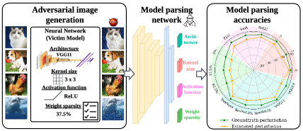
Figure 1: Schematic overview of victim model parsing from adversarial attacks. (Left) Attack generation based on victim model (with model attributes, architecture type, kernel size, activation function, and weight sparsity). (Middle) Proposed model parsing network (MPN) that assigns VM attribute class to input adversarial data. (Right) Highlighted results: The accuracy of model parsing from PGD attacks [11] against ResNet9 on CIFAR-10. Here the performance of MPN is reported under two different input data formats, the true adversarial perturbations and the estimated adversarial perturbations (proposed in Sec. 4).

We call problem (Q) model parsing of adversarial attacks; see Fig. 1 for an illustration. This is also inspired by the model parsing problem defined for generative model (GM) [40], which attempts to infer model hyperparameters of GM from synthesized photo-realistic images. However, adversarial attacks are data-specific input perturbations determined by hand-crafted optimizers rather than GM. And the ‘model attributes’ to be parsed from adversarial attacks are associated with the VM (victim model), which has a weaker correlation with attacked data compared to synthesized images by GM. The latter is easier to encode data-independent GM attribute information [39, 40, 42, 43, 44].

The significance of the proposed model parsing problem can also be demonstrated through a transfer attack example (Fig. 2). Suppose that adversarial attacks are generated from model A but used as transfer attacks against model B. If model parsing is possible, we will then be able to infer the true victim model source of these adversarial instances and shed light on the hidden model attributes.

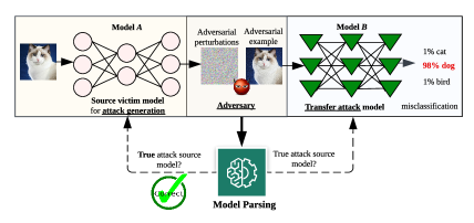
Figure 2: Motivating example on model parsing of transfer attack. A successful model parsing module can reveal the true source victim model.

Contributions.

We summarize our contributions below.

$\bullet$ We propose and formalize the problem of model parsing to infer VM attributes from a variety of adversarial attacks.

$\bullet$ We approach the model parsing problem of adversarial attacks as a supervised learning task and show that the learned model parsing network (MPN) could exhibit a surprising amount of generalization to recognize VM attributes from testing attack instances (see Fig. 1 for highlighted results). We also peer into the influence of designing factors (including input data format, backbone network, and evaluation metric) in MPN’s generalization.

$\bullet$ We make a comprehensive empirical study on the feasibility and effectiveness of model parsing from adversarial attacks, including the in-distribution generalization on unseen adversarial images as well as the out-of-distribution generalization on unseen attack types and model architectures. We also demonstrate how the model parsing approach can be used to uncover the true, source victim model attributes from transfer attacks (Fig. 2), and show a connection between model parsing and attack transferability.

2 Related Work

Adversarial attacks and defenses.

Intensive research efforts have been made for the design of adversarial attacks and defenses. Adversarial attacks in the digital domain [2, 12, 11, 13, 56, 57, 19, 15, 14, 17, 21, 58, 59] typically deceive DNNs by integrating carefully-crafted tiny perturbations into input data. Adversarial attacks in the physical domain [60, 61, 62, 63, 64, 65] are further developed to fool victim models under complex physical environmental conditions, which require stronger adversarial perturbations than digital attacks. In this work, we focus on the commonly-used digital attacks subject to $\ell_{p}$-norm based perturbation constraints, known as $\ell_{p}$ attacks for $p\in\{2,\infty\}$. Based on how an adversary interacts with the VM (victim model), $\ell_{p}$ attacks also include both white-box attacks (with full access to the victim model based on which attacks are generated) and black-box attacks (with access only to the victim model’s input and output). The former typically leverages the local gradient information of VM to generate attacks [2, 12, 11], while the latter takes input-output queries of VM in attack generation; Examples include score-based attacks [15, 14, 17] and decision-based attacks [21, 58, 59].

Given the vulnerability of ML models to adversarial attacks, methods to defend against these attacks are now a major focus in research [11, 22, 23, 24, 25, 26, 27, 37, 28, 29, 30, 31, 32, 33, 46, 66, 36, 34, 35, 47, 67]. One line of research focuses on advancing model training methods to learn adversarially robust models [11, 22, 23, 24, 25, 26, 27, 37, 67]. Examples include min-max optimization-based adversarial training and its many variants [11, 22, 25, 26, 27, 37], which can equip models with empirical robustness. To make models provably robust, certified training is also developed by integrating robustness certificate regularization into model training [68, 69, 23] or leveraging randomized smoothing [24, 70, 71]. In addition to training robust models, another line of research on adversarial defense is to detect adversarial attacks by exploring and exploiting the differences between adversarial data and benign data [28, 29, 30, 31, 32, 33, 46, 66].

Reverse engineering of deception (RED).

RED has emerged as a new adversarial learning to defend against adversarial attacks and infer the adversary’s knowledge (such as its identifications, attack objectives, and attack perturbations). For example, a few recent works [48, 50, 55, 28, 54] aim to reverse engineer the type of attack generation method and the used hyperparameters (e.g., perturbation radius and step number). In addition, other works focus on estimating or attributing the adversarial perturbations used to construct adversarial images [49, 51, 52, 53]. This line of research also relates to adversarial purification [36, 34, 35, 47], the technique to defend against adversarial attacks by characterizing and removing their harmful influence in model predictions.

However, none of the prior works investigated if VM attributes are invertible from adversarial attacks. That is, the proposed model parsing problem remains open in adversarial learning. If feasible, the insight into model parsing could offer us an in-depth understanding of the encountered threat model and inspire new designs of adversarial defenses and robust models. Our work is also inspired by the model parsing problem in GM (generative model) [40], aiming to infer GM attributes from their synthesized images. The rationale is that GM often encodes model fingerprints in synthesized images so that these fingerprints can be leveraged for DeepFake detection and model parsing [39, 40, 42, 43, 44]. Lastly, we stress that RED is different from the work [72, 73] on reverse engineering of (black-box) model hyperparameters, which estimates model attributes from the model’s prediction logits. However, in this work VM is unknown for model parsing of adversarial attacks, and the only information we have is the dataset of attack instances.

3 Preliminaries and Problem Setups

Preliminaries: Adversarial attacks and victim models.

We first introduce different kinds of adversarial attacks and exhibit their dependence on VM (victim model), i.e., the ML model from which attacks are generated. Throughout the paper, we will focus on $\ell_{p}$ attacks, where the adversary aims to generate imperceptible input perturbations to fool an image classifier [2]. Let $\mathbf{x}$ and $\boldsymbol{\theta}$ denote a benign image and the parameters of VM. The adversarial attack (a.k.a, adversarial example) is defined via the linear perturbation model $\mathbf{x}^{\prime}=\mathbf{x}+\boldsymbol{\delta}$, where $\boldsymbol{\delta}=\mathcal{A}(\mathbf{x},\boldsymbol{\theta},\epsilon)$ denotes adversarial perturbations, and $\mathcal{A}$ refers to an attack generation method relying on $\mathbf{x}$, $\boldsymbol{\theta}$, and the attack strength $\epsilon$ (i.e., the perturbation radius of $\ell_{p}$ attacks).

We focus on 7 attack methods given their different dependencies on the victim model ($\boldsymbol{\theta}$), including input gradient-based white-box attacks with full access to $\boldsymbol{\theta}$ (FGSM [2], PGD [11], CW [12], and AutoAttack or AA [13]) as well as query-based black-box attacks (ZO-signSGD [15], NES [16], and SquareAttack or Square [17]).

✦ FGSM (fast gradient sign method) [2]: This attack method is given by $\boldsymbol{\delta}=\mathbf{x}-\epsilon\times\mathrm{sign}(\nabla_{\mathbf{x}}\ell_{\mathrm{atk}}(\mathbf{x};\boldsymbol{\theta}))$, where $\mathrm{sign}(\cdot)$ is the entry-wise sign operation, and $\nabla_{\mathbf{x}}\ell_{\mathrm{atk}}$ is the input gradient of an attack loss $\ell_{\mathrm{atk}}(\mathbf{x};\boldsymbol{\theta})$ evaluated at $\mathbf{x}$ under $\boldsymbol{\theta}$.

✦ PGD (projected gradient descent) [11]: This extends FGSM via an iterative algorithm. Formally, the $K$-step PGD $\ell_{\infty}$ attack is given by $\boldsymbol{\delta}=\boldsymbol{\delta}_{K}$, where $\boldsymbol{\delta}_{k}=\mathcal{P}_{\|\boldsymbol{\delta}\|_{\infty}\leq\epsilon}(\boldsymbol{\delta}_{k-1}-\alpha\times\mathrm{sign}(\nabla_{\mathbf{x}}\ell_{\mathrm{atk}}(\mathbf{x};\boldsymbol{\theta})))$ for $k=1,\ldots,K$, $\mathcal{P}_{\|\boldsymbol{\delta}\|_{\infty}\leq\epsilon}$ is the projection operation onto the $\ell_{\infty}$-norm constraint $\|\boldsymbol{\delta}\|_{\infty}\leq\epsilon$, and $\alpha$ is the attack step size. By replacing the $\ell_{\infty}$ norm with the $\ell_{2}$ norm, we similarly obtain the PGD $\ell_{2}$ attack [11].

✦ CW (Carlini-Wager) attack [12]: Similar to PGD, CW calls iterative optimization for attack generation. Yet, CW formulates attack generation as an $\ell_{p}$-norm regularized optimization problem, with the regularization parameter $c=1$ by default. For example, the choice of $c=1$ in CW $\ell_{2}$ attack could lead to a variety of perturbation strengths with the average value around $\epsilon=0.33$ on the CIFAR-10 dataset. Moreover, CW adopts a hinge loss to ensure the misclassification margin. We will focus on CW $\ell_{2}$ attack.

✦ AutoAttack (or AA) [13]: This is an ensemble attack that uses AutoPGD, an adaptive version of PGD, as the primary means of attack. The loss of AutoPGD is given by the difference of logits ratio (DLR) rather than CE or CW loss.

✦ ZO-signSGD [15] and NES [16]: They are zeroth-order optimization (ZOO)-based black-box attacks. Different from the aforementioned white-box gradient-based attacks, the only interaction mode of black-box attacks with the victim model ($\boldsymbol{\theta}$) is submitting inputs and receiving the corresponding predicted outputs. ZOO then uses these input-output queries to estimate input gradients and generate adversarial perturbations. Yet, ZO-signSGD and NES call different gradient estimators in ZOO [74].

✦ SquareAttack (or Square) [17]: This attack is built upon random search and thus does not rely on input gradient.

Table 1: Summary of adversarial attack types focused in this work. Here GD refers to gradient descent, and WB and BB refer to white-box and black-box dependence on the victim model, respectively.

Attacks	Generation method	Loss	$\ell_{p}$ norm	Strength $\epsilon$	Dependence on $\boldsymbol{\theta}$
FGSM	one-step GD	CE	$\ell_{\infty}$	{4, 8, 12, 16}/255	WB, gradient-based
PGD	multi-step GD	CE	$\ell_{\infty}$	{4, 8, 12, 16}/255	WB, gradient-based
			$\ell_{2}$	0.25, 0.5, 0.75, 1
CW	multi-step GD	CW	$\ell_{2}$	soft regularization $c\in\{0.1,1,10\}$	WB, gradient-based
AutoAttack	attack ensemble	CE /	$\ell_{\infty}$	{4, 8, 12, 16}/255	WB, gradient-based +
or AA		DLR	$\ell_{2}$	0.25, 0.5, 0.75, 1	BB, query-based
SquareAttack	random search	CE	$\ell_{\infty}$	{4, 8, 12, 16}/255	BB, query-based
or Square			$\ell_{2}$	0.25, 0.5, 0.75, 1
NES	ZOO	CE	$\ell_{\infty}$	{4, 8, 12, 16}/255	BB, query-based
ZO-signSGD	ZOO	CE	$\ell_{\infty}$	{4, 8, 12, 16}/255	BB, query-based

Although there exist other types of $\ell_{p}$ attacks, our focused attack methods have been diverse, covering different optimization methods, attack losses, $\ell_{p}$ norms, and dependencies on the VM $\boldsymbol{\theta}$, as summarized in Table 1.

Model parsing of adversarial attacks.

It is clear that adversarial attacks contain the information of VM ($\boldsymbol{\theta}$), although the degree of their dependence varies. Inspired by the above, one may wonder if the attributes of $\boldsymbol{\theta}$ can be inferred from these attack instances, i.e., adversarial perturbations, or perturbed images. The model attributes of our interest include model architecture types as well as finer-level knowledge, e.g., activation function type. We call the resulting problem model parsing of adversarial attacks, as described below.

rgb]0.85,0.9,0.95 (Problem statement) Is it possible to infer victim model information from adversarial attacks? And what factors will influence such model parsing ability?

To our best knowledge, the feasibility of model parsing from adversarial attack instances is an open question. Its challenges stay in two dimensions. First, through the model lens, VM (victim model) is indirectly coupled with adversarial attacks, e.g., via local gradient information or model queries. Thus, it remains elusive what VM information is fingerprinted in adversarial attacks and impacts the feasibility of model parsing. Second, through the attack lens, the diversity of adversarial attacks (Table 1) makes a once-for-all model parsing solution extremely difficult. Spurred by the above, we will take the first solid step to investigate the feasibility of model parsing from adversarial attacks and study what factors may influence the model parsing performance. The insight into model parsing could offer us an in-depth understanding of the encountered threat model and inspire new designs of adversarial defenses and robust models.

Table 2: Summary of model attributes of interest. Each attribute value corresponds to an attribute class in model parsing.

Model attributes	Code	Classes per attribute
Architecture type	AT	ResNet9, ResNet18
		ResNet20, VGG11, VGG13
Kernel size	KS	3, 5, 7
Activation function	AF	ReLU, tanh, ELU
Weight sparsity	WS	0%, 37.5%, 62.5%

Model attributes and setup.

We specify VMs of adversarial attacks as convolutional neural network (CNN)-based image classifiers. More concretely, we consider 5 CNN architecture types (ATs): ResNet9, ResNet18, ResNet20, VGG11, and VGG13. Given an AT, CNN models are then configured by different choices of kernel size (KS), activation function (AF), and weight sparsity (WS). Thus, a valued quadruple (AT, KS, AF, WS) yields a specific VM ($\boldsymbol{\theta}$). Although more attributes could be considered, the rationale behind our choices is given below. We focus on KS and AF since they are the two fundamental building components of CNNs. Besides, we choose WS as another model attribute since it relates to sparse models achieved by pruning (i.e., removing redundant model weights) [75, 76]. We defer sanity checks of all-dimension model attributes for future studies.

Table 2 summarizes the focused model attributes and their values to specify VM instances. Given a VM specification, we generate adversarial attacks following attack methods in Table 1. Unless specified otherwise, our empirical studies will be mainly given on CIFAR-10 but experiments on other datasets will also be provided in Sec. 5.

4 Methods

In this section, we approach the model parsing problem as a standard supervised learning task applied over the dataset of adversarial attacks. We will show that the learned model parsing network could exhibit a surprising amount of generalization on test-time adversarial data. We will also show data-model factors that may influence such generalization.

Model parsing network and training.

We approach the model parsing problem as a supervised attribute recognition task. That is, we develop a parametric model, termed model parsing network (MPN), which takes adversarial attacks as input and predicts the model attribute values (i.e., ‘classes’ in Table 2). Despite the simplicity of supervised learning, the construction of MPN is non-trivial when designing data format, backbone network, and evaluation metrics.

We first create a model parsing dataset by collecting adversarial attack instances against victim models. Since adversarial attacks are proposed for evading model predictions in the post-training stage, we choose the test set of an ordinary image dataset (e.g., CIFAR-10) to generate adversarial data, where an 80/20 training/test split is used for MPN training and evaluation. Following notations in Sec. 3, the training set of MPN is denoted by $\mathcal{D}_{\mathrm{tr}}=\{(\mathbf{z}(\mathcal{A},\mathbf{x},\boldsymbol{\theta}),y(\boldsymbol{\theta}))\,|\,\mathbf{x}\in\mathcal{I}_{\mathrm{tr}},\boldsymbol{\theta}\in\Theta\}$, where $\mathbf{z}$ signifies an attack data feature (e.g., adversarial perturbations $\boldsymbol{\delta}$ or adversarial example $\mathbf{x}^{\prime}$) that relies on the attack method $\mathcal{A}$, the original image sample $\mathbf{x}$, and the VM $\boldsymbol{\theta}$, and $y(\boldsymbol{\theta})$ denotes the true model attribute label associated with $\boldsymbol{\theta}$. To differentiate with the testing data of MPN, we denote by $\mathcal{I}_{\mathrm{tr}}$ the set of original images used for training MPN. We also denote by $\Theta$ the set of model architectures used for generating attack data in $\mathcal{D}_{\mathrm{tr}}$. For ease of presentation, we express the training set of MPN as $\mathcal{D}_{\mathrm{tr}}=\{(\mathbf{z},y)\}$ to omit the dependence on other factors.

Next, we elaborate on the construction of MPN (parameterized by $\boldsymbol{\phi}$). We intend to make the architecture of MPN as simple as possible and make it different from the VM $\boldsymbol{\theta}$. The rationale behind that has two folds. First, we would like to examine the feasibility of model parsing from adversarial attacks even forcing the simplicity of attribution network ($\boldsymbol{\phi}$). Second, we would like to avoid the ‘model attribute bias’ of $\boldsymbol{\phi}$ when inferring VM attributes from adversarial attacks. Inspired by the above, we specify MPN by two simple networks: (1) multilayer perceptron (MLP) containing two hidden layers with 128 hidden units (0.41M parameters) [77], and (2) a simple 4-layer CNN (ConvNet-4) with 64 output channels for each layer, followed by one fully-connected layers with 128 hidden units and the attribution prediction head (0.15M parameters) [78]. As will be evident later (Fig. 4), the model parsing accuracy of ConvNet-4 typically outperforms that of MLP. Thus, ConvNet-4 will be used as the MPN model by default.

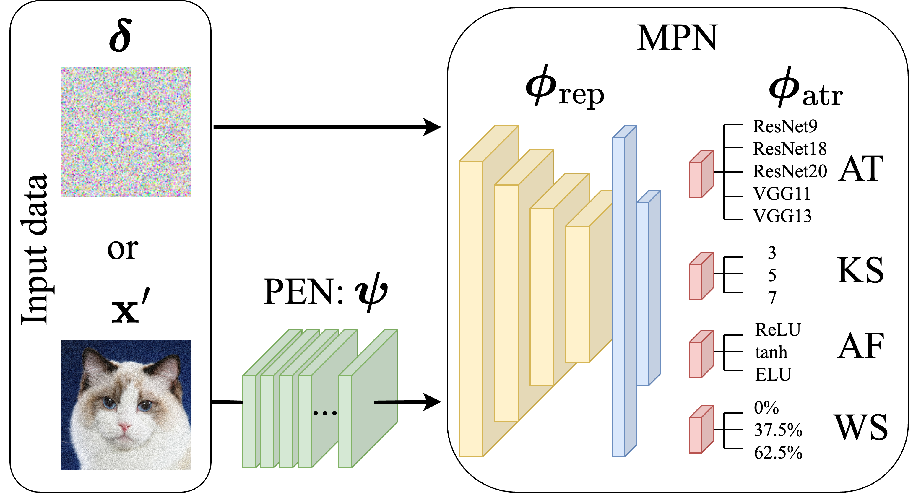
Figure 3: The schematic overview of our proposal. Here PEN (perturbation estimation network) will be introduced later as a pre-processing step to transform adversarial examples into perturbation-alike input data.

Given the datamodel setup, we next tackle the recognition problem of VM’s attributes (AT, KS, AF, WS) via a multi-head multi-class classifier. We dissect MPN into two parts $\boldsymbol{\phi}=[{\boldsymbol{\phi}}_{\text{rep}},\boldsymbol{\phi}_{\text{atr}}]$, where ${\boldsymbol{\phi}}_{\text{rep}}$ is for data representation acquisition, and ${\boldsymbol{\phi}}_{\text{attr}}$ corresponds to the attribute-specific prediction head (i.e., the last fully-connected layer in our design). Eventually, four prediction heads $\{\boldsymbol{\phi}_{\text{atr}}^{(i)}\}_{i=1}^{4}$ will share ${\boldsymbol{\phi}}_{\text{rep}}$ for model attribute recognition; see Fig. 3 for a schematic overview of our proposal. The MPN training problem is then cast as

$$\begin{array}[]{l}\displaystyle\operatorname*{\text{minimize}}_{{\boldsymbol{\phi}}_{\text{rep}},\{\boldsymbol{\phi}_{\text{atr}}^{(i)}\}_{i=1}^{4}}\mathbb{E}_{(\mathbf{z},y)\in\mathcal{D}_{\mathrm{tr}}}\sum_{i=1}^{4}[\ell_{\mathrm{CE}}(h(\mathbf{z};{\boldsymbol{\phi}}_{\text{rep}},\boldsymbol{\phi}_{\text{atr}}^{(i)}),y_{i})],\end{array}$$ (2)

where $h(\mathbf{z};{\boldsymbol{\phi}}_{\text{rep}},\boldsymbol{\phi}_{\text{atr}}^{(i)})$ denotes the MPN prediction at input example $\mathbf{z}$ using the predictive model consisting of ${\boldsymbol{\phi}}_{\text{rep}}$ and $\boldsymbol{\phi}_{\text{atr}}^{(i)}$ for the $i$th attribute classification, $y_{i}$ is the ground-truth label of the $i$th attribute associated with the input data $\mathbf{z}$, and $\ell_{\mathrm{CE}}$ is the cross-entropy (CE) loss characterizing the error between the prediction and the true label.

Evaluation methods.

Similar to training, we denote by $\mathcal{D}_{\mathrm{test}}=\{(\mathbf{z}(\mathcal{A},\mathbf{x},\boldsymbol{\theta}),y(\boldsymbol{\theta}))\,|\,\mathbf{x}\in\mathcal{I}_{\mathrm{test}},\boldsymbol{\theta}\in\Theta\}$ the test attack set for evaluating the performance of MPN. Here the set of benign images $\mathcal{I}_{\mathrm{test}}$ is different from $\mathcal{I}_{\mathrm{tr}}$, thus adversarial attacks in $\mathcal{D}_{\mathrm{test}}$ are new to $\mathcal{D}_{\mathrm{tr}}$. To mimic the standard evaluation pipeline of supervised learning, we propose the following evaluation metrics.

(1) In-distribution generalization: The MPN testing dataset $\mathcal{D}_{\mathrm{test}}$ follows the attack methods ($\mathcal{A}$) and the VM specifications ($\Theta$) same as $\mathcal{D}_{\mathrm{tr}}$ but corresponding to different original benign images (i.e., $\mathcal{I}_{\mathrm{test}}\neq\mathcal{I}_{\mathrm{tr}}$). The purpose of such an in-distribution evaluation is to examine if the trained MPN can infer model attributes encoded in new attack data given already-seen attack methods.

(2) Out-of-distribution (OOD) generalization: In addition to new test-time images, there could exist attack/model distribution shifts in $\mathcal{D}_{\mathrm{test}}$ due to using new attack methods or model architectures, leading to unseen attack methods ($\mathcal{A}$) and victim models ($\Theta$) different from the settings in $\mathcal{D}_{\mathrm{tr}}$.

In the rest of the paper, both in-distribution and OOD generalization capabilities will be assessed. Unless specified otherwise, the generalization of MPN stands for the in-distribution generalization.

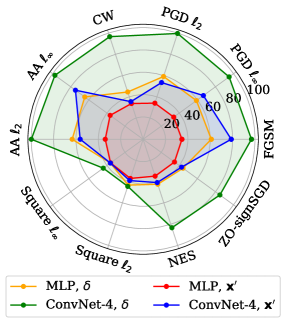
Figure 4: The in-distribution generalization of MPN using different formats of input data (adversarial perturbations $\boldsymbol{\delta}$ vs. adversarial examples $\mathbf{x}^{\prime}$) and parsing networks (ConvNet-4 vs. MLP). The generalization performance is measured by the averaged testing accuracy of attribute-specific classifiers; see Sec. 5.1. The attack data are generated from 10 attack methods given in Table 1, with $\ell_{\infty}$ attack strength $\epsilon=8/255$ and $\ell_{2}$ attack strength $\epsilon=0.5$ on CIFAR-10. The VM architecture is fixed to ResNet-9, and VM instances are generated by varying other model attributes in Table 2.

Perturbations or adversarial examples? The input data format matters for MPN.

Recall from Sec. 3 that an adversarial example, given by the linear model $\mathbf{x}^{\prime}=\mathbf{x}+\boldsymbol{\delta}$, relates to $\boldsymbol{\theta}$ through $\boldsymbol{\delta}$. Thus, it could be better for MPN to adopt adversarial perturbations ($\boldsymbol{\delta}$) as the attack data feature ($\mathbf{z}$), rather than the indirect adversarial example $\mathbf{x}^{\prime}$. Fig. 4 empirically justifies our hypothesis by comparing the generalization of MPN trained on adversarial perturbations with that on adversarial examples under two model specifications of MPN, MLP and ConvNet-4. We present the performance of MPN trained and tested on different attack types. As we can see, the use of adversarial perturbations ($\boldsymbol{\delta}$) consistently improves the test-time classification accuracy of VM attributes, compared to the use of adversarial examples ($\mathbf{x}^{\prime}$). In addition, ConvNet-4 outperforms MLP with a substantial margin.

Although Fig. 4 shows the promise of the generalization ability of MPN when trained and tested on adversarial perturbations, it may raise another practical question of how to obtain adversarial perturbations from adversarial examples if the latter is the only attack source accessible to MPN. To overcome this difficulty, we propose a perturbation estimator network (PEN) that can be jointly learned with MPN. Once PEN is prepended to the MPN model, the resulting end-to-end pipeline can achieve model parsing using adversarial examples as inputs (see Fig. 3). We use a denoising network, DnCNN [79], to model PEN with parameters $\boldsymbol{\psi}$. PEN obtains perturbation estimates by minimizing the denoising objective function using the true adversarial perturbations as supervision. Extended from (2), we then have

$$\begin{array}[]{ll}\displaystyle\operatorname*{\text{minimize}}_{\boldsymbol{\psi},{\boldsymbol{\phi}}_{\text{rep}},\{\boldsymbol{\phi}_{\text{atr}}^{(i)}\}_{i=1}^{4}}&\beta\mathbb{E}_{(\mathbf{x},\mathbf{x}^{\prime})\in\mathcal{D}_{\mathrm{tr}}}[\ell_{\mathrm{MAE}}(g_{\boldsymbol{\psi}}(\mathbf{x}^{\prime}),\mathbf{x}^{\prime}-\mathbf{x})]\\ &+\mathbb{E}_{(\mathbf{x}^{\prime},y)\in\mathcal{D}_{\mathrm{tr}}}\sum_{i=1}^{4}[\ell_{\mathrm{CE}}(h(g_{\boldsymbol{\psi}}(\mathbf{x}^{\prime});{\boldsymbol{\phi}}_{\text{rep}},\boldsymbol{\phi}_{\text{atr}}^{(i)}),y_{i})],\end{array}$$ (5)

where $g_{\boldsymbol{\psi}}(\mathbf{x}^{\prime})$ is the output of PEN given $\mathbf{x}^{\prime}$ as the input, $\ell_{\mathrm{MAE}}$ is the mean-absolute-error (MAE) loss characterizing the perturbation estimation error, and $\beta>0$ is a regularization parameter. Compared with (2), MPN takes the perturbation estimate $g_{\boldsymbol{\psi}}(\mathbf{x}^{\prime})$ for VM attribute classification.

5 Experiments

5.1 Experiment setup and implementation

Dataset curation.

We use standard image classification datasets (CIFAR-10, CIFAR-100, and Tiny-ImageNet) to acquire victim models, from which attacks are generated. We refer readers to Appendix A for details on victim model training and evaluation, as well as different attack setups. These VM instances are then leveraged to create MPN datasets (as described in Sec. 4). The attack types and victim model configurations have been summarized in Table 1 and 2. Thus, we collect a dataset consisting of adversarial attacks across $7$ attack types generated from $135$ VMs (configured by $5$ architecture types, $3$ kernel size setups, $3$ activation function types, and $3$ weight sparsity levels).

MPN training and evaluation.

To solve problem (2), we train the MPN model using the SGD (stochastic gradient descent) optimizer with cosine annealing learning rate schedule and an initial learning rate of $0.1$. The training epoch number and the batch sizes are given by $100$ and $256$, respectively. To solve problem (5), we first train MPN according to (2), and then fine-tune a pre-trained DnCNN model [49] (taking only the denoising objective into consideration) for 20 epochs. Starting from these initial models, we jointly optimize MPN and PEN by minimizing problem (5) with $\beta=1$ over 50 epochs. To evaluate the effectiveness of MPN, we consider both in-distribution and OOD generalization assessment. The generalization performance is measured by testing accuracy averaged over attribute-wise predictions, namely, $\sum_{i}(N_{i}\mathrm{TA}(i))/\sum_{i}N_{i}$, where $N_{i}$ is the number of classes of the model attribute $i$, and $\mathrm{TA}(i)$ is the testing accuracy of the classifier associated with the attribute $i$ (Fig. 3).

5.2 Results and insights

In-distribution generalization of MPN is achievable.

Table 3 presents the in-distribution generalization performance of MPN trained using different input data formats (i.e., adversarial examples $\mathbf{x}^{\prime}$, PEN-estimated adversarial perturbations $\boldsymbol{\delta}_{\text{{\text{PEN}}}}$, and true adversarial perturbations $\boldsymbol{\delta}$) given each attack type in Table 1. Here the choice of AT (architecture type) is fixed to ResNet9, but adversarial attacks on CIFAR-10 are generated from VMs configured by different values of KS, AF, and WS (see Table 2). As we can see, the generalization of MPN varies against the attack type even if model parsing is conducted from the ideal adversarial perturbations ($\boldsymbol{\delta}$). We also note that model parsing from white-box adversarial attacks (i.e., FGSM, PGD, and AA) is easier than that from black-box attacks (i.e., ZO-signSGD, NES, and Square). For example, the worst-case performance of MPN is achieved when training/testing on Square attacks. This is not surprising, since Square is based on random search and has the least dependence on VM attributes. In addition, we find that MPN using estimated perturbations ($\boldsymbol{\delta}_{\mathrm{PEN}}$) substantially outperforms the one trained on adversarial examples ($\mathbf{x}^{\prime}$). This justifies the effectiveness of our proposed PEN solution for MPN.

Table 3: The in-distribution testing accuracy (%) of MPN trained using different input data formats (adversarial examples $\mathbf{x}^{\prime}$, PEN-estimated adversarial perturbations $\boldsymbol{\delta}_{\text{{\text{PEN}}}}$, and true adversarial perturbations $\boldsymbol{\delta}$) across different attack types on CIFAR-10, with $\ell_{\infty}$ attack strength $\epsilon=8/255$, $\ell_{2}$ attack strength $\epsilon=0.5$, and CW attack strength $c=1$.

	FGSM	PGD $\ell_{\infty}$	PGD $\ell_{2}$	CW	AA $\ell_{\infty}$	AA $\ell_{2}$	Square $\ell_{\infty}$	Square $\ell_{2}$	NES	ZO- signSGD
$\mathbf{x}^{\prime}$	78.80	66.62	53.42	35.42	74.78	56.26	38.92	36.21	40.80	42.48
$\boldsymbol{\delta}_{{\text{PEN}}}$	94.15	83.20	82.58	64.46	91.09	86.89	44.14	42.30	58.85	61.20
$\boldsymbol{\delta}$	96.89	95.07	99.64	96.66	97.48	99.95	44.37	44.05	83.33	84.87

Table 4: In-distribution generalization performance (testing accuracy, %) of MPN given different choices of VMs and datasets, attack types/strengths, and MPN input data formats ($\mathbf{x}^{\prime}$, $\boldsymbol{\delta}_{\mathrm{PEN}}$, and $\boldsymbol{\delta}$).

Attack type	Attack strength	Dataset and victim model
		CIFAR-10 ResNet9			CIFAR-10 ResNet18			CIFAR-10 ResNet20			CIFAR-10 VGG11			CIFAR-10 VGG13			CIFAR-100 ResNet9			Tiny-ImageNet ResNet18
		$\mathbf{x}^{\prime}$	$\boldsymbol{\delta}_{\mathrm{PEN}}$	$\boldsymbol{\delta}$	$\mathbf{x}^{\prime}$	$\boldsymbol{\delta}_{\mathrm{PEN}}$	$\boldsymbol{\delta}$	$\mathbf{x}^{\prime}$	$\boldsymbol{\delta}_{\mathrm{PEN}}$	$\boldsymbol{\delta}$	$\mathbf{x}^{\prime}$	$\boldsymbol{\delta}_{\mathrm{PEN}}$	$\boldsymbol{\delta}$	$\mathbf{x}^{\prime}$	$\boldsymbol{\delta}_{\mathrm{PEN}}$	$\boldsymbol{\delta}$	$\mathbf{x}^{\prime}$	$\boldsymbol{\delta}_{\mathrm{PEN}}$	$\boldsymbol{\delta}$	$\mathbf{x}^{\prime}$	$\boldsymbol{\delta}_{\mathrm{PEN}}$	$\boldsymbol{\delta}$
FGSM	$\epsilon=4/255$	60.13	85.25	96.82	60.00	86.92	97.66	62.41	88.91	97.64	47.42	73.40	91.75	66.28	90.02	98.57	57.99	82.22	94.86	37.23	84.27	97.04
	$\epsilon=8/255$	78.80	94.15	96.89	80.44	95.49	97.61	82.29	95.90	97.72	63.13	86.76	92.41	84.92	96.91	98.66	75.58	91.65	94.96	70.29	91.17	97.05
	$\epsilon=12/255$	86.49	95.96	96.94	88.03	96.89	97.68	88.71	97.13	97.81	73.71	90.19	92.66	91.21	98.10	98.71	82.27	94.01	95.55	76.00	93.45	97.02
	$\epsilon=16/255$	90.16	96.43	96.94	91.71	97.34	97.68	91.84	97.47	97.79	79.51	91.28	92.60	94.22	98.44	98.73	86.50	94.04	94.74	79.63	94.35	96.87
PGD $\ell_{\infty}$	$\epsilon=4/255$	50.54	76.43	96.02	56.94	79.45	96.96	55.01	80.05	97.49	39.33	66.38	91.84	57.12	81.18	98.29	42.27	72.62	92.65	35.48	76.56	97.18
	$\epsilon=8/255$	66.62	83.20	95.07	73.29	87.29	95.38	67.49	86.19	96.18	56.62	81.14	92.78	69.16	88.46	97.22	59.71	79.55	90.43	61.85	82.90	96.05
	$\epsilon=12/255$	76.65	89.73	94.91	81.73	91.67	95.55	76.41	90.16	95.67	70.56	88.92	94.13	78.67	92.93	97.26	70.86	85.31	91.28	73.82	88.80	96.38
	$\epsilon=16/255$	75.58	86.95	91.28	82.46	90.19	93.19	76.58	87.79	92.50	72.13	87.23	91.85	78.28	90.20	94.66	71.29	82.35	86.84	73.19	85.02	93.54
PGD $\ell_{2}$	$\epsilon=0.25$	36.75	62.20	99.66	46.35	70.17	99.74	48.24	77.22	99.75	36.47	45.17	98.52	35.81	70.62	99.85	35.92	61.91	99.29	35.55	35.68	99.68
	$\epsilon=0.5$	53.42	82.58	99.64	60.89	84.70	99.56	61.62	89.11	99.61	41.56	66.58	98.68	57.83	87.64	99.83	48.89	79.26	99.01	35.52	54.56	99.71
	$\epsilon=0.75$	62.66	89.04	99.48	71.01	89.89	99.22	70.76	92.06	99.36	47.02	78.12	98.52	72.76	92.32	99.74	59.19	85.14	98.61	35.56	81.33	99.71
	$\epsilon=1$	71.65	91.73	99.26	77.09	92.09	98.94	76.84	92.82	98.96	54.20	84.30	98.41	79.93	93.96	99.57	66.97	87.63	97.89	43.48	88.81	99.64
CW	$c=0.1$	33.77	55.60	96.71	47.77	63.26	96.11	33.56	63.11	94.10	33.73	48.90	94.37	33.68	65.48	96.95	34.41	46.47	92.55	35.96	35.77	95.52
	$c=1$	35.42	64.46	96.66	45.75	65.25	97.45	33.74	62.71	97.08	33.89	55.61	91.29	36.12	68.66	98.58	34.25	55.18	93.25	35.54	35.29	89.35
	$c=10$	36.38	64.45	96.64	45.83	65.32	97.41	33.83	63.52	97.11	38.29	56.83	91.33	38.51	68.28	98.62	34.25	55.89	93.18	35.45	53.18	94.20

Extended from Table 3, Fig. 5 shows the generalization performance of MPN when evaluated using attack data with different attack strengths. We observe that in-distribution generalization (corresponding to the same attack strength for the train-time and test-time attacks) is easier to achieve than OOD generalization (different attack strengths at test time and train time). Another observation is that a smaller gap between the train-time attack strength and the test-time strength leads to better generalization performance.

  

Figure 5: Testing accuracies (%) of MPN when trained on adversarial perturbations generated by PGD $\ell_{\infty}$ using different attack strengths ($\epsilon$) and evaluated using different attack strengths as well. Other setups are consistent with in Table 3.

Table 3 and Fig. 5 focused on model parsing of adversarial attacks by fixing the VM architecture to ResNet9 on CIFAR-10, although different model attribute combinations lead to various ResNet9-type VM instantiations for attack generation. Furthermore, Table 4 shows the in-distribution generalization of MPN under diverse setups of victim model architectures and datasets. The insights into model parsing are consistent with Table 3: (1) The use of true adversarial perturbations ($\boldsymbol{\delta}$) and PEN-estimated perturbations ($\boldsymbol{\delta}_{\mathrm{PEN}}$) can yield higher model parsing accuracy. And (2) inferring model attributes from white-box, gradient-based adversarial perturbations is easier, as supported by its over 90% testing accuracy. We also observe that if adversarial examples ($\mathbf{x}^{\prime}$) or estimated adversarial perturbations ($\boldsymbol{\delta}_{\text{{\text{PEN}}}}$) are used for model parsing, then the resulting accuracy gets better if adversarial attacks have a higher attack strength.

OOD generalization of MPN becomes difficult vs. unseen, dissimilar attack types at testing time.

In Fig. 6, we present the generalization matrix of MPN when trained under one attack type (e.g., PGD $\ell_{\infty}$ attack at row $1$) but tested under another attack type (e.g., FGSM attack at column $2$) when adversarial perturbations are generated from the same set of ResNet9-based VMs (with different configurations of other model attributes) on CIFAR-10. The diagonal entries of the matrix correspond to the in-distribution generalization of MPN given the attack type, while the off-diagonal entries characterize OOD generalization when the test-time attack type is different from the train-time one.

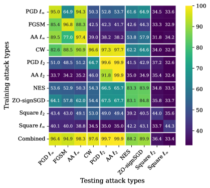
Figure 6: Generalization performance (%) matrix of MPN when trained on a row-specific attack type but evaluated on a column-specific attack type. The attack data are given by adversarial perturbations with strength $\epsilon=8/255$ for $\ell_{\infty}$ attacks, $\epsilon=0.5$ for $\ell_{2}$ attacks, and $c=1$ for CW attack. The VM architecture and the dataset are set to ResNet9 and CIFAR-10. The ‘combined’ row represents MPN training on the collection of four attack types: PGD $\ell_{\infty}$, PGD $\ell_{2}$, CW, and ZO-signSGD.

First, we find that MPN generalizes better across attack types when they share similarities, leading to the following generalization communities: $\ell_{\infty}$ attacks (PGD $\ell_{\infty}$, FGSM, and AA $\ell_{\infty}$), $\ell_{2}$ attacks (CW, PGD $\ell_{2}$, or AA $\ell_{2}$), and ZOO-based black-box attacks (NES and ZO-signSGD). Second, Square attacks are difficult to learn and generalize, as evidenced by the low test accuracies in the last two rows and the last two columns. This is also consistent with Table 3. Third, given the existence of generalization communities, we then combine diverse attack types (including PGD $\ell_{\infty}$, PGD $\ell_{2}$, CW, and ZO-signSGD) into an augmented MPN training set and investigate if such a data augmentation can boost the OOD generalization of MPN. The results are summarized in the ‘combined’ row of Fig. 6. As we expect, the use of combined attack types indeed makes MPN generalize better across all attack types except for the random search-based Square attack. In Fig. A1 of Appendix B, we also find the consistent OOD generalization performance of MPN when PEN-based adversarial perturbations are used in MPN.

Fig. 7 demonstrates the generalization matrix of MPN when trained and evaluated using adversarial perturbations generated from different VM architectures (i.e., different values of AT in Table 1) by fixing the configurations of other attributes (KS, AF, and WS). We observe that given an attack type, the in-distribution MPN generalization remains well across VM architectures. Yet, the OOD generalization of MPN (corresponding to the off-diagonal entries of the generalization matrix) rapidly degrades if the test-time VM architecture is different from the train-time one. Thus, if MPN is trained on data with AT classes as supervision, then the in-distribution generalization on AT retains. We refer readers to Appendix C for more results for AT prediction.

     (a) FGSM (b) PGD $\ell_{\infty}$ (c) CW

Figure 7: Generalization matrix (%) of MPN when trained on attack data generated from a row-specific architecture but evaluated on attack data generated from a column-specific architecture. Both the train-time and test-time architectures share the same VM attributes in KS, AF, and WS. The attack type is specified by FGSM, PGD $\ell_{\infty}$, or CW on CIFAR-10, with the attack strength $\epsilon=8/255$ for $\ell_{\infty}$ attacks and $c=1$ for CW.

MPN to uncover real VM attributes of transfer attacks.

As a use case of model parsing, we next investigate if MPN can correctly infer the source VM attributes from transfer attacks when applied to attacking a different model (see Fig. 2). Given the VM architecture ResNet9, we vary the values of model attributes KS, AF, and WS to produce $27$ ResNet9-type VMs. Fig. 8 shows the transfer attack success rate (ASR) matrix (Fig. 8a) and the model parsing confusion matrix (Fig. 8b). Here the attack type is given by PGD $\ell_{\infty}$ attack with strength $\epsilon=8/255$ on CIFAR-10, and the resulting adversarial perturbations (generated from different VMs) are used for MPN training and evaluation.

In Fig. 8a, the off-diagonal entries represent ASRs of transfer attacks from row-wise VMs to attacking column-wise target models. As we can see, adversarial attacks generated from the ReLU-based VMs are typically more difficult to transfer to smooth activation function (ELU or tanh)-based target models. By contrast, given the values of KS and AF, attacks are easier to transfer across models with different weight sparsity levels.

Fig. 8b presents the confusion matrix of MPN trained on attack data generated from all $27$ ResNet9-alike VMs. Each row of the confusion matrix represents the true VM used to generate the attack dataset, and each column corresponds to a predicted model attribute configuration. Thus, the diagonal entries and the off-diagonal entries in Fig. 8b represent the correct model parsing accuracy and the misclassification rate on the incorrectly predicted model attribute configuration. As we can see, attacks generated from ReLU-based VMs result in a low misclassification rate of MPN on ELU or tanh-based predictions (see the marked region ①). Meanwhile, a high misclassification occurs for MPN when evaluated on attack data corresponding to different values of WS (see the marked region ②). The above results, together with our insights into ASRs of transfer attacks in Fig. 8a, suggest a connection between transfer attack and model parsing: If attacks are difficult (or easy) to transfer from the source model to the target model, then inferring the source model attributes from these attacks turns to be easy (or difficult).

(a) Attack successful rate (%) (b) Confusion matrix (%)

Figure 8: Model parsing of transfer attacks: Transfer attack success rate matrix (a) and model parsing confusion matrix (b). Given the architecture type ResNet9, the dataset CIFAR-10, and the attack type PGD $\ell_{\infty}$ (with strength $\epsilon=8/255$), each model attribute combination (AF, KS, WS) defines a model instance to be attacked, transferred, or parsed.

Model parsing vs. model robustness.

Further, we examine the influence of adversarial robustness of victim models in the generalization performance of MPN; see Fig. A2 in Appendix D. We find that adversarial attacks against robust VMs is harder to parse VM attributes than attacks against standard VMs.

6 Conclusion

We studied the model parsing problem of adversarial attacks to infer victim model attributes, and approached this problem as a supervised learning task by training a model parsing network (MPN). We studied both in-distribution and out-of-distribution generalization of MPN considering unseen attack types and model architectures. We demystified several key factors, such as input data formats, backbone network choices, and VM characteristics (like attack transferability and robustness), which can influence the effectiveness of model parsing. Extensive experiments are provided to demonstrate when, how, and why victim model information can be inferred from adversarial attacks.

7 Acknowledgement

The work was supported by the DARPA RED program.

Appendix

Appendix A Victim model training, evaluation, and attack setups

When training all CIFAR-10, CIFAR-100, and Tiny-ImageNet victim models (each of which is given by an attribute combination), we use the SGD optimizer with the cosine annealing learning rate schedule and an initial learning rate of 0.1. The weight decay is $5e-4$, and the batch size is 256. The number of training epochs is 75 for CIFAR-10 and CIFAR-100, and 100 for Tiny-ImageNet. When the weight sparsity (WS) is promoted, we follow the one-shot magnitude pruning method [76, 80] to obtain a sparse model. To obtain models with different activation functions (AF) and kernel sizes (KS), we modify the convolutional block design in the ResNet and VGG model family accordingly from 3, ReLU to others, i.e., 5/7, tanh/ELU. Table A1 shows the testing accuracy (%) of victim models on different datasets, given any studied (AF, KS, WS) tuple included in Table 2. It is worth noting that we accelerate victim model training by using FFCV [81] when loading the dataset.

Table A1: Victim model performance (testing accuracy, %) given different choices of datasets and model architectures.

Dataset	AT	Attribute combination
		ReLU									tanh									ELU
		3			5			7			3			5			7			3			5			7
		0%	37.5%	62.5%	0%	37.5%	62.5%	0%	37.5%	62.5%	0%	37.5%	62.5%	0%	37.5%	62.5%	0%	37.5%	62.5%	0%	37.5%	62.5%	0%	37.5%	62.5%	0%	37.5%	62.5%
CIFAR-10	ResNet9	94.4	93.9	94.2	93.3	93.5	93.5	92.4	92.8	92.8	89.0	88.8	89.9	88.4	88.6	88.2	87.0	87.2	88.0	91.0	91.2	90.7	90.3	90.2	90.5	89.3	90.0	89.6
	ResNet18	94.7	94.9	95.0	94.2	94.5	94.5	93.9	93.5	93.6	87.1	87.5	88.2	84.2	84.9	85.5	81.3	81.2	85.1	90.6	90.8	90.6	90.1	91.1	90.5	85.7	83.4	84.3
	ResNet20	92.1	92.5	92.3	92.0	92.2	92.0	90.9	91.8	91.5	89.7	89.7	89.7	89.5	89.4	89.6	88.3	88.2	88.9	90.7	91.2	90.9	90.3	90.5	90.6	89.2	89.7	89.7
	VGG11	91.0	91.1	90.4	89.8	89.9	89.4	88.2	88.4	88.0	88.7	89.1	88.9	87.2	87.6	87.6	87.0	86.8	87.0	89.4	89.5	89.5	88.0	88.2	88.5	87.1	87.1	87.2
	VGG13	93.1	93.3	93.0	92.0	92.2	92.6	91.2	91.1	91.0	90.1	90.1	90.1	89.3	89.1	89.3	88.2	88.8	88.8	90.8	90.9	90.8	89.2	89.5	89.4	88.4	88.7	88.9
CIFAR-100	ResNet9	73.3	73.6	73.5	71.8	71.9	71.2	69.1	69.8	69.2	58.6	60.1	60.3	60.1	61.2	62.0	58.2	59.8	60.3	70.8	70.7	70.8	69.5	69.6	69.8	67.3	68.3	68.7
	ResNet18	74.4	75.0	75.6	73.6	73.0	74.6	71.2	71.0	70.9	62.0	62.0	62.9	57.3	59.3	60.1	51.3	53.4	57.1	70.1	70.8	71.1	66.8	69.7	69.7	63.1	61.8	65.7
	ResNet20	68.3	68.4	67.5	67.8	67.5	67.7	66.8	66.7	67.6	59.9	61.3	59.6	61.9	62.0	62.1	59.9	61.2	61.2	66.4	67.6	67.7	67.0	67.3	67.2	66.2	66.9	66.8
	VGG11	68.3	68.4	67.7	65.2	65.7	65.8	62.4	62.0	62.6	65.2	65.5	65.5	63.6	63.6	63.9	62.1	61.8	62.5	66.2	66.5	65.9	64.6	64.0	64.6	61.5	62.3	61.9
	VGG13	71.0	70.6	71.1	69.9	70.5	70.3	66.5	66.5	67.2	66.7	67.5	67.5	65.2	65.5	67.1	63.9	63.4	65.0	68.9	69.3	69.5	66.3	66.7	67.1	64.2	64.5	64.7
Tiny-ImageNet	ResNet18	63.7	64.1	63.5	61.5	62.7	62.6	59.6	61.0	61.7	47.0	48.1	50.0	46.6	47.9	48.3	41.0	43.5	44.6	57.2	57.9	58.1	52.7	53.8	53.6	52.3	51.5	52.3

For different attack types, we list all the attack configurations below:

✦ FGSM. We set the attack strength $\epsilon$ equal to $4/255$, $8/255$, $12/255$, and $16/255$, respectively.

✦ PGD $\ell_{\infty}$. We set the attack step number equal to 10, and the attack strength-learning rate combinations as ($\epsilon=4/255$, $\alpha=0.5/255$), ($\epsilon=8/255$, $\alpha=1/255$), ($\epsilon=12/255$, $\alpha=2/255$), and ($\epsilon=16/255$, $\alpha=2/255$).

✦ PGD $\ell_{2}$. We set the step number equal to 10, and the attack strength-learning rate combinations as ($\epsilon=0.25$, $\alpha=0.05$), ($\epsilon=0.5$, $\alpha=0.1$), ($\epsilon=0.75$, $\alpha=0.15$), and ($\epsilon=1.0$, $\alpha=0.2$).

✦ CW. We use $\ell_{2}$ version CW attack with the attack conference parameter $\kappa$ equal to $0$. We also set the learning rate equal to $0.01$ and the maximum iteration number equal to $50$ to search for successful attacks.

✦ AutoAttack $\ell_{\infty}$. We use the standard version of AutoAttack with the $\ell_{\infty}$ norm and $\epsilon$ equal to $4/255$, $8/255$, $12/255$, and $16/255$, respectively.

✦ AutoAttack $\ell_{2}$. We use the standard version of AutoAttack with the $\ell_{2}$ norm and $\epsilon$ equal to $0.25$, $0.5$, $0.75$, and $1.0$, respectively.

✦ SquareAttack $\ell_{\infty}$. We set the maximum query number equal to $5000$ with $\ell_{\infty}$ norm $\epsilon$ equal to $4/255$, $8/255$, $12/255$, and $16/255$, respectively.

✦ SquareAttack $\ell_{2}$. We set the maximum query number equal to $5000$ with $\ell_{\infty}$ norm $\epsilon$ equal to $0.25$, $0.5$, $0.75$, and $1.0$, respectively.

✦ NES. We set the query number for each gradient estimate equal to 10, together with $\mu=0.01$ (i.e., the value of the smoothing parameter to obtain the finite difference of function evaluations). We also set the learning rate by $0.0005$, and the maximum iteration number by 500 for each adversarial example generation.

✦ ZO-signSGD. We set the query number for each gradient estimate equal to 10 with $\mu=0.01$. We also set the learning rate equal to $0.0005$, and the maximum iteration number equal to 500 for each adversarial example generation. The only difference between ZO-signSGD and NES is the gradient estimation method in ZOO. ZO-signSGD uses the sign of forward difference-based estimator while NES uses the central difference-based estimator.

Appendix B OOD generalization performance of MPN across attack types when PEN is used

Similar to Fig. 8, Fig. A1 shows the generalization performance of MPN when trained on a row-specific attack type but evaluated on a column-specific attack type when $\boldsymbol{\delta}_{\text{PEN}}$ is given as input. When MPN is trained on the collection of four attack types PGD $\ell_{\infty}$, PGD $\ell_{2}$, CW, and ZO-signSGD (i.e., the ‘Combined’ row), such a data augmentation can boost the OOD generalization except for the random search-based Square attack.

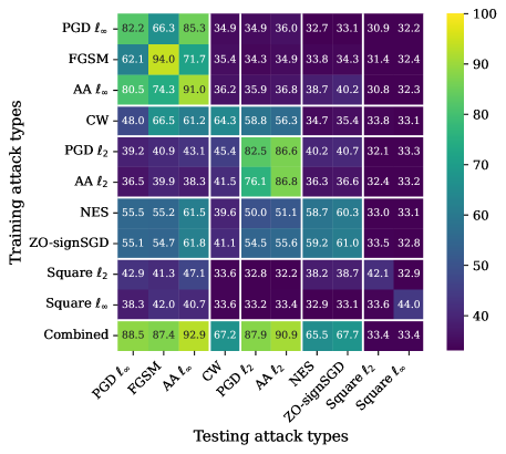
Figure A1: Generalization performance matrix of MPN when trained on a row-specific attack type but evaluated on a column-specific attack type given $\boldsymbol{\delta}_{{\text{PEN}}}$ as input. The attack data are given by adversarial perturbations with strength $\epsilon=8/255$ for $\ell_{\infty}$ attacks, $\epsilon=0.5$ for $\ell_{2}$ attacks, and $c=1$ for CW attack. The victim model architecture and the dataset are set as ResNet9 and CIFAR-10. The ‘combined’ row represents MPN training on the collection of four attack types: PGD $\ell_{\infty}$, PGD $\ell_{2}$, CW, and ZO-signSGD.

Appendix C MPN for architecture type (AT) prediction

MPN is also trained on (AT, AF, KS, WS) tuple by merging AT into the attribute classification task. We conduct experiments considering different architectures mentioned in Table 2 on CIFAR-10 and CIFAR-100, with $\boldsymbol{\delta}$ and $\boldsymbol{\delta}_{\text{PEN}}$ as MPN’s inputs, respectively. We summarize the in-distribution generalization results in Table A2, Table A3, Table A4, and Table A5. Weighted accuracy refers to the testing accuracy defined in Sec. 5, i.e., $\sum_{i}(N_{i}\mathrm{TA}(i))/\sum_{i}N_{i}$, where $N_{i}$ is the number of classes of the model attribute $i$, and $\mathrm{TA}(i)$ is the testing accuracy of the classifier associated with the attribute $i$ (Fig. 3). In the above tables, we also show the testing accuracy for each attribute, i.e., $\mathrm{TA}(i)$. Combined accuracy refers to the testing accuracy over all victim model attribute-combined classes, i.e., 135 classes for 5 AT classes, 3 AF classes, 3 KS classes, and 3 WS classes. The insights into model parsing are summarized below: (1) MPN trained on $\boldsymbol{\delta}$ and $\boldsymbol{\delta}_{{\text{PEN}}}$ can effectively classify all the attributes AT, AF, KS, WS in terms of per-attribute classification accuracy, weighted testing accuracy, and combined accuracy. (2) Compared to AT, AF, and KS, WS is harder to parse.

Table A2: MPN performance (%) on different attack types given different evaluation metrics with adversarial perturbation $\boldsymbol{\delta}$ as input on CIFAR-10.

Metrics	Attack types
	FGSM				PGD $\ell_{\infty}$				PGD $\ell_{2}$				CW
	$\epsilon=4/255$	$\epsilon=8/255$	$\epsilon=12/255$	$\epsilon=16/255$	$\epsilon=4/255$	$\epsilon=8/255$	$\epsilon=12/255$	$\epsilon=16/255$	$\epsilon=0.25$	$\epsilon=0.5$	$\epsilon=0.75$	$\epsilon=1.0$	$c=0.1$	$c=1$	$c=10$
AT accuracy	97.77	97.85	97.91	97.91	97.23	96.13	96.16	94.22	99.77	99.64	99.37	99.12	96.73	97.30	97.28
AF accuracy	95.67	95.73	95.79	95.71	95.86	95.26	95.77	94.05	99.51	99.36	99.04	98.68	95.12	94.84	94.68
KS accuracy	98.66	98.66	98.65	98.71	98.22	97.55	97.43	95.52	99.83	99.79	99.64	99.48	96.94	98.13	98.09
WS accuracy	87.16	87.16	87.29	87.52	84.36	79.99	80.01	71.68	98.51	97.83	96.86	95.57	88.42	85.28	85.03
Weighted accuracy	95.24	95.28	95.34	95.38	94.39	92.79	92.89	89.63	99.46	99.23	98.82	98.34	94.65	94.38	94.27
Combined accuracy	81.85	82.00	82.19	82.33	78.65	73.11	73.33	62.67	97.79	96.89	95.38	93.55	83.00	79.29	78.88

Table A3: MPN performance (%) on different attack types given different evaluation metrics with estimated perturbation $\boldsymbol{\delta}_{\text{PEN}}$ as input on CIFAR-10.

Metrics	Attack types
	FGSM				PGD $\ell_{\infty}$				PGD $\ell_{2}$				CW
	$\epsilon=4/255$	$\epsilon=8/255$	$\epsilon=12/255$	$\epsilon=16/255$	$\epsilon=4/255$	$\epsilon=8/255$	$\epsilon=12/255$	$\epsilon=16/255$	$\epsilon=0.25$	$\epsilon=0.5$	$\epsilon=0.75$	$\epsilon=1.0$	$c=0.1$	$c=1$	$c=10$
AT accuracy	88.98	95.68	97.20	97.64	75.81	84.58	90.27	88.50	61.09	81.41	87.80	90.48	56.10	64.11	64.30
AF accuracy	83.48	92.21	94.56	95.22	74.95	85.04	90.72	89.81	57.62	76.90	83.95	87.36	54.61	58.77	58.98
KS accuracy	91.57	96.63	97.96	98.41	81.10	88.18	92.67	90.99	67.85	84.50	89.93	92.18	62.46	69.81	70.15
WS accuracy	69.99	81.42	84.92	86.59	56.07	63.92	70.19	64.80	50.09	67.26	74.02	77.70	46.40	47.53	47.77
Weighted accuracy	84.29	92.08	94.17	94.92	72.53	81.02	86.58	84.23	59.44	78.07	84.48	87.44	55.07	60.63	60.87
Combined accuracy	54.83	72.66	78.63	80.83	32.59	46.05	57.10	50.60	18.38	45.39	57.10	63.00	14.62	19.44	19.70

Table A4: MPN performance (%) on different attack types given different evaluation metrics with adversarial perturbation $\boldsymbol{\delta}$ as input on CIFAR-100.

Metrics	Attack types
	FGSM				PGD $\ell_{\infty}$				PGD $\ell_{2}$				CW
	$\epsilon=4/255$	$\epsilon=8/255$	$\epsilon=12/255$	$\epsilon=16/255$	$\epsilon=4/255$	$\epsilon=8/255$	$\epsilon=12/255$	$\epsilon=16/255$	$\epsilon=0.25$	$\epsilon=0.5$	$\epsilon=0.75$	$\epsilon=1.0$	$c=0.1$	$c=1$	$c=10$
AT accuracy	97.70	97.76	97.76	97.75	97.03	95.40	95.23	92.52	99.59	99.29	98.91	98.50	93.84	96.23	96.30
AF accuracy	95.17	95.14	94.96	95.11	94.79	93.73	93.87	91.87	99.14	98.63	97.97	97.31	90.83	92.32	92.47
KS accuracy	97.66	97.65	97.69	97.62	96.75	95.16	94.44	91.25	99.62	99.43	99.16	98.70	93.11	95.77	95.81
WS accuracy	81.13	80.77	80.90	80.94	76.57	69.85	68.16	59.42	96.58	95.04	92.70	90.43	76.61	74.64	74.77
Weighted accuracy	93.60	93.54	93.53	93.55	92.11	89.52	88.97	85.02	98.85	98.27	97.43	96.56	89.34	90.67	90.76
Combined accuracy	75.08	74.76	74.82	74.95	69.72	61.27	59.31	48.37	95.27	93.06	89.89	86.73	67.19	66.24	66.56

Table A5: MPN performance (%) on different attack types given different evaluation metrics with estimated perturbation $\boldsymbol{\delta}_{\text{PEN}}$ as input on CIFAR-100.

Metrics	Attack types
	FGSM				PGD $\ell_{\infty}$				PGD $\ell_{2}$				CW
	$\epsilon=4/255$	$\epsilon=8/255$	$\epsilon=12/255$	$\epsilon=16/255$	$\epsilon=4/255$	$\epsilon=8/255$	$\epsilon=12/255$	$\epsilon=16/255$	$\epsilon=0.25$	$\epsilon=0.5$	$\epsilon=0.75$	$\epsilon=1.0$	$c=0.1$	$c=1$	$c=10$
AT accuracy	88.17	95.25	96.92	97.45	72.40	82.48	88.11	85.47	62.77	80.01	85.88	88.33	47.31	51.80	52.48
AF accuracy	81.81	91.14	93.53	94.52	71.43	81.93	87.76	86.71	58.16	74.06	80.88	84.18	49.98	49.49	49.96
KS accuracy	88.62	94.92	96.58	97.12	76.97	84.74	88.78	86.46	69.38	84.09	88.68	90.56	56.07	59.68	59.72
WS accuracy	64.19	74.98	78.60	79.85	50.64	56.88	60.32	54.94	46.50	61.73	67.79	70.59	39.46	39.85	40.37
Weighted accuracy	81.76	89.95	92.19	92.98	68.51	77.36	82.22	79.40	59.71	75.69	81.53	84.12	48.08	50.43	50.90
Combined accuracy	47.75	65.27	71.05	73.27	25.56	37.49	45.28	38.97	16.27	38.87	49.04	54.06	7.31	9.20	9.59

Appendix D Model parsing vs. model robustness

We re-use the collected ResNet9-type victim models in Fig. 8, and obtain their adversarially robust versions by conducting adversarial training [11] on CIFAR-10. Fig. A2 presents the generalization matrix of MPN when trained on a row-wise attack type but evaluated on a column-wise attack type. Yet, different from Fig. 6, the considered attack type is expanded by incorporating ‘attack against robust model’, besides ‘attack against standard model’. It is worth noting that every attack type corresponds to attack data generated from victim models (VMs) instantiated by the combinations of model attributes KS, AF, and WS. Thus, the diagonal entries and the off-diagonal entries of the generalization matrix in Fig. A2 reflect the in-distribution parsing accuracy within an attack type and the OOD generalization across attack types. Here are two key observations. First, the in-distribution generalization of MPN from attacks against robust VMs is much poorer (see the marked region ①), compared to that from attacks against standard VMs. Second, the off-diagonal performance shows that MPN trained on attacks against standard VMs is harder to parse model attributes from attacks against robust VMs, and vice versa (see the marked region ②). Based on the above results, we posit that model parsing is easier for attacks generated from VMs with higher accuracy and lower robustness.

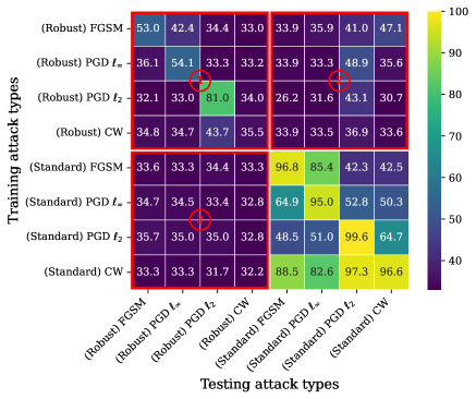
Figure A2: Generalization performance (%) matrix of MPN across attack types, ranging from FGSM, PGD $\ell_{\infty}$, PGD $\ell_{2}$, and CW attacks against standard victim models to their variants against robust victim models, termed (Standard or Robust) Attack. Other setups are consistent with Fig. 6.

References

- [1] Christian Szegedy, Wojciech Zaremba, Ilya Sutskever, Joan Bruna, Dumitru Erhan, Ian Goodfellow, and Rob Fergus. Intriguing properties of neural networks. arXiv preprint arXiv:1312.6199, 2013.
- [2] Ian J Goodfellow, Jonathon Shlens, and Christian Szegedy. Explaining and harnessing adversarial examples. arXiv preprint arXiv:1412.6572, 2014.
- [3] Cihang Xie, Jianyu Wang, Zhishuai Zhang, Yuyin Zhou, Lingxi Xie, and Alan Yuille. Adversarial examples for semantic segmentation and object detection. In Proceedings of the IEEE international conference on computer vision, pages 1369–1378, 2017.
- [4] James Tu, Mengye Ren, Sivabalan Manivasagam, Ming Liang, Bin Yang, Richard Du, Frank Cheng, and Raquel Urtasun. Physically realizable adversarial examples for lidar object detection. In Proceedings of the IEEE/CVF Conference on Computer Vision and Pattern Recognition, pages 13716–13725, 2020.
- [5] Vegard Antun, Francesco Renna, Clarice Poon, Ben Adcock, and Anders C Hansen. On instabilities of deep learning in image reconstruction and the potential costs of ai. Proceedings of the National Academy of Sciences, 117(48):30088–30095, 2020.
- [6] Ankit Raj, Yoram Bresler, and Bo Li. Improving robustness of deep-learning-based image reconstruction. In International Conference on Machine Learning, pages 7932–7942. PMLR, 2020.
- [7] Ziyu Jiang, Tianlong Chen, Ting Chen, and Zhangyang Wang. Robust pre-training by adversarial contrastive learning. Advances in neural information processing systems, 33:16199–16210, 2020.
- [8] Lijie Fan, Sijia Liu, Pin-Yu Chen, Gaoyuan Zhang, and Chuang Gan. When does contrastive learning preserve adversarial robustness from pretraining to finetuning? Advances in neural information processing systems, 34:21480–21492, 2021.
- [9] Rishi Bommasani, Drew A Hudson, Ehsan Adeli, Russ Altman, Simran Arora, Sydney von Arx, Michael S Bernstein, Jeannette Bohg, Antoine Bosselut, Emma Brunskill, et al. On the opportunities and risks of foundation models. arXiv preprint arXiv:2108.07258, 2021.
- [10] Natalie Maus, Patrick Chao, Eric Wong, and Jacob Gardner. Adversarial prompting for black box foundation models. arXiv preprint arXiv:2302.04237, 2023.
- [11] Aleksander Madry, Aleksandar Makelov, Ludwig Schmidt, Dimitris Tsipras, and Adrian Vladu. Towards deep learning models resistant to adversarial attacks. arXiv preprint arXiv:1706.06083, 2017.
- [12] Nicholas Carlini and David Wagner. Towards evaluating the robustness of neural networks. In 2017 ieee symposium on security and privacy (sp), pages 39–57. Ieee, 2017.
- [13] Francesco Croce and Matthias Hein. Reliable evaluation of adversarial robustness with an ensemble of diverse parameter-free attacks. In International conference on machine learning, pages 2206–2216. PMLR, 2020.
- [14] Pin-Yu Chen, Huan Zhang, Yash Sharma, Jinfeng Yi, and Cho-Jui Hsieh. Zoo: Zeroth order optimization based black-box attacks to deep neural networks without training substitute models. In Proceedings of the 10th ACM Workshop on Artificial Intelligence and Security, pages 15–26. ACM, 2017.
- [15] Sijia Liu, Pin-Yu Chen, Xiangyi Chen, and Mingyi Hong. signSGD via zeroth-order oracle. In International Conference on Learning Representations, 2019.
- [16] Andrew Ilyas, Logan Engstrom, Anish Athalye, and Jessy Lin. Black-box adversarial attacks with limited queries and information. In International conference on machine learning, pages 2137–2146. PMLR, 2018.
- [17] Maksym Andriushchenko, Francesco Croce, Nicolas Flammarion, and Matthias Hein. Square attack: a query-efficient black-box adversarial attack via random search. In Computer Vision–ECCV 2020: 16th European Conference, Glasgow, UK, August 23–28, 2020, Proceedings, Part XXIII, pages 484–501. Springer, 2020.
- [18] Cihang Xie, Zhishuai Zhang, Yuyin Zhou, Song Bai, Jianyu Wang, Zhou Ren, and Alan L Yuille. Improving transferability of adversarial examples with input diversity. In Proceedings of the IEEE/CVF Conference on Computer Vision and Pattern Recognition, pages 2730–2739, 2019.
- [19] Chaowei Xiao, Jun-Yan Zhu, Bo Li, Warren He, Mingyan Liu, and Dawn Song. Spatially transformed adversarial examples. In International Conference on Learning Representations, 2018.
- [20] Seyed-Mohsen Moosavi-Dezfooli, Alhussein Fawzi, and Pascal Frossard. Deepfool: a simple and accurate method to fool deep neural networks. In Proceedings of the IEEE conference on computer vision and pattern recognition, pages 2574–2582, 2016.
- [21] Wieland Brendel, Jonas Rauber, and Matthias Bethge. Decision-based adversarial attacks: Reliable attacks against black-box machine learning models. arXiv preprint arXiv:1712.04248, 2017.
- [22] Hongyang Zhang, Yaodong Yu, Jiantao Jiao, Eric P Xing, Laurent El Ghaoui, and Michael I Jordan. Theoretically principled trade-off between robustness and accuracy. ICML, 2019.
- [23] Eric Wong and J Zico Kolter. Provable defenses against adversarial examples via the convex outer adversarial polytope. arXiv preprint arXiv:1711.00851, 2017.
- [24] Hadi Salman, Mingjie Sun, Greg Yang, Ashish Kapoor, and J Zico Kolter. Denoised smoothing: A provable defense for pretrained classifiers. NeurIPS, 2020.
- [25] Eric Wong, Leslie Rice, and J Zico Kolter. Fast is better than free: Revisiting adversarial training. arXiv preprint arXiv:2001.03994, 2020.
- [26] Yair Carmon, Aditi Raghunathan, Ludwig Schmidt, John C Duchi, and Percy S Liang. Unlabeled data improves adversarial robustness. In Advances in Neural Information Processing Systems (NeurIPS), 2019.
- [27] Ali Shafahi, Mahyar Najibi, Mohammad Amin Ghiasi, Zheng Xu, John Dickerson, Christoph Studer, Larry S Davis, Gavin Taylor, and Tom Goldstein. Adversarial training for free! In Advances in Neural Information Processing Systems, pages 3353–3364, 2019.
- [28] Mo Zhou and Vishal M Patel. On trace of pgd-like adversarial attacks. arXiv preprint arXiv:2205.09586, 2022.
- [29] Kathrin Grosse, Praveen Manoharan, Nicolas Papernot, Michael Backes, and Patrick McDaniel. On the (statistical) detection of adversarial examples. arXiv preprint arXiv:1702.06280, 2017.
- [30] Puyudi Yang, Jianbo Chen, Cho-Jui Hsieh, Jane-Ling Wang, and Michael Jordan. Ml-loo: Detecting adversarial examples with feature attribution. In Proceedings of the AAAI Conference on Artificial Intelligence (AAAI), 2020.
- [31] Jan Hendrik Metzen, Tim Genewein, Volker Fischer, and Bastian Bischoff. On detecting adversarial perturbations. arXiv preprint arXiv:1702.04267, 2017.
- [32] Dongyu Meng and Hao Chen. Magnet: a two-pronged defense against adversarial examples. In Proceedings of the 2017 ACM SIGSAC Conference on Computer and Communications Security, pages 135–147. ACM, 2017.
- [33] Bartosz Wójcik, Paweł Morawiecki, Marek Śmieja, Tomasz Krzyżek, Przemysław Spurek, and Jacek Tabor. Adversarial examples detection and analysis with layer-wise autoencoders. arXiv preprint arXiv:2006.10013, 2020.
- [34] Changhao Shi, Chester Holtz, and Gal Mishne. Online adversarial purification based on self-supervision. arXiv preprint arXiv:2101.09387, 2021.
- [35] Jongmin Yoon, Sung Ju Hwang, and Juho Lee. Adversarial purification with score-based generative models. In International Conference on Machine Learning, pages 12062–12072. PMLR, 2021.
- [36] Vignesh Srinivasan, Csaba Rohrer, Arturo Marban, Klaus-Robert Müller, Wojciech Samek, and Shinichi Nakajima. Robustifying models against adversarial attacks by langevin dynamics. Neural Networks, 137:1–17, 2021.
- [37] Yihua Zhang, Guanhua Zhang, Prashant Khanduri, Mingyi Hong, Shiyu Chang, and Sijia Liu. Revisiting and advancing fast adversarial training through the lens of bi-level optimization. In International Conference on Machine Learning, pages 26693–26712. PMLR, 2022.
- [38] Yimeng Zhang, Yuguang Yao, Jinghan Jia, Jinfeng Yi, Mingyi Hong, Shiyu Chang, and Sijia Liu. How to robustify black-box ML models? a zeroth-order optimization perspective. In International Conference on Learning Representations, 2022.
- [39] Sheng-Yu Wang, Oliver Wang, Richard Zhang, Andrew Owens, and Alexei A Efros. Cnn-generated images are surprisingly easy to spot… for now. In Proceedings of the IEEE/CVF conference on computer vision and pattern recognition, pages 8695–8704, 2020.
- [40] Vishal Asnani, Xi Yin, Tal Hassner, and Xiaoming Liu. Reverse engineering of generative models: Inferring model hyperparameters from generated images. arXiv preprint arXiv:2106.07873, 2021.
- [41] Prafulla Dhariwal and Alexander Nichol. Diffusion models beat gans on image synthesis. Advances in Neural Information Processing Systems, 34:8780–8794, 2021.
- [42] Ning Yu, Larry S Davis, and Mario Fritz. Attributing fake images to gans: Learning and analyzing gan fingerprints. In Proceedings of the IEEE/CVF international conference on computer vision, pages 7556–7566, 2019.
- [43] Joel Frank, Thorsten Eisenhofer, Lea Schönherr, Asja Fischer, Dorothea Kolossa, and Thorsten Holz. Leveraging frequency analysis for deep fake image recognition. In International conference on machine learning, pages 3247–3258. PMLR, 2020.
- [44] Luca Guarnera, Oliver Giudice, and Sebastiano Battiato. Deepfake detection by analyzing convolutional traces. In Proceedings of the IEEE/CVF conference on computer vision and pattern recognition workshops, pages 666–667, 2020.
- [45] Tarik Dzanic, Karan Shah, and Freddie Witherden. Fourier spectrum discrepancies in deep network generated images. Advances in neural information processing systems, 33:3022–3032, 2020.
- [46] Fangzhou Liao, Ming Liang, Yinpeng Dong, Tianyu Pang, Xiaolin Hu, and Jun Zhu. Defense against Adversarial Attacks Using High-Level Representation Guided Denoiser. arXiv:1712.02976 [cs], May 2018.
- [47] Weili Nie, Brandon Guo, Yujia Huang, Chaowei Xiao, Arash Vahdat, and Anima Anandkumar. Diffusion models for adversarial purification. arXiv preprint arXiv:2205.07460, 2022.
- [48] David Aaron Nicholson and Vincent Emanuele. Reverse engineering adversarial attacks with fingerprints from adversarial examples. arXiv preprint arXiv:2301.13869, 2023.
- [49] Yifan Gong, Yuguang Yao, Yize Li, Yimeng Zhang, Xiaoming Liu, Xue Lin, and Sijia Liu. Reverse engineering of imperceptible adversarial image perturbations. arXiv preprint arXiv:2203.14145, 2022.
- [50] Xiawei Wang, Yao Li, Cho-Jui Hsieh, and Thomas Chun Man Lee. CAN MACHINE TELL THE DISTORTION DIFFERENCE? a REVERSE ENGINEERING STUDY OF ADVERSARIAL ATTACKS, 2023.
- [51] Michael Goebel, Jason Bunk, Srinjoy Chattopadhyay, Lakshmanan Nataraj, Shivkumar Chandrasekaran, and BS Manjunath. Attribution of gradient based adversarial attacks for reverse engineering of deceptions. arXiv preprint arXiv:2103.11002, 2021.
- [52] Hossein Souri, Pirazh Khorramshahi, Chun Pong Lau, Micah Goldblum, and Rama Chellappa. Identification of attack-specific signatures in adversarial examples. arXiv preprint arXiv:2110.06802, 2021.
- [53] Darshan Thaker, Paris Giampouras, and René Vidal. Reverse engineering attacks: A block-sparse optimization approach with recovery guarantees. In International Conference on Machine Learning, pages 21253–21271. PMLR, 2022.
- [54] Zhongyi Guo, Keji Han, Yao Ge, Wei Ji, and Yun Li. Scalable attribution of adversarial attacks via multi-task learning. arXiv preprint arXiv:2302.14059, 2023.
- [55] Pratyush Maini, Xinyun Chen, Bo Li, and Dawn Song. Perturbation type categorization for multiple $\ell_p$ bounded adversarial robustness, 2021.
- [56] Kaidi Xu, Sijia Liu, Pu Zhao, Pin-Yu Chen, Huan Zhang, Quanfu Fan, Deniz Erdogmus, Yanzhi Wang, and Xue Lin. Structured adversarial attack: Towards general implementation and better interpretability. In ICLR, 2019.
- [57] Pin-Yu Chen, Yash Sharma, Huan Zhang, Jinfeng Yi, and Cho-Jui Hsieh. EAD: elastic-net attacks to deep neural networks via adversarial examples. In Proceedings of the AAAI Conference on Artificial Intelligence, pages 10–17, 2018.
- [58] Minhao Cheng, Simranjit Singh, Patrick Chen, Pin-Yu Chen, Sijia Liu, and Cho-Jui Hsieh. Sign-opt: A query-efficient hard-label adversarial attack. arXiv preprint arXiv:1909.10773, 2019.
- [59] Jinghui Chen and Quanquan Gu. Rays: A ray searching method for hard-label adversarial attack. In Proceedings of the 26th ACM SIGKDD International Conference on Knowledge Discovery & Data Mining, pages 1739–1747, 2020.
- [60] K. Eykholt, I. Evtimov, E. Fernandes, B. Li, A. Rahmati, C. Xiao, A. Prakash, T. Kohno, and D. Song. Robust physical-world attacks on deep learning visual classification. In Proceedings of the Conference on Computer Vision and Pattern Recognition (CVPR), 2018.
- [61] Juncheng Li, Frank Schmidt, and Zico Kolter. Adversarial camera stickers: A physical camera-based attack on deep learning systems. In International Conference on Machine Learning, pages 3896–3904, 2019.
- [62] A. Athalye, L. Engstrom, A. Ilyas, and K. Kwok. Synthesizing robust adversarial examples. In ICML, 2018.
- [63] Shang-Tse Chen, Cory Cornelius, Jason Martin, and Duen Horng Polo Chau. Shapeshifter: Robust physical adversarial attack on faster r-cnn object detector. In Joint European Conference on Machine Learning and Knowledge Discovery in Databases, pages 52–68. Springer, 2018.
- [64] Kaidi Xu, Gaoyuan Zhang, Sijia Liu, Quanfu Fan, Mengshu Sun, Hongge Chen, Pin-Yu Chen, Yanzhi Wang, and Xue Lin. Evading real-time person detectors by adversarial t-shirt. arXiv preprint arXiv:1910.11099, 2019.
- [65] Donghua Wang, Wen Yao, Tingsong Jiang, Guijiang Tang, and Xiaoqian Chen. A survey on physical adversarial attack in computer vision. arXiv preprint arXiv:2209.14262, 2022.
- [66] Kaidi Xu, Sijia Liu, Gaoyuan Zhang, Mengshu Sun, Pu Zhao, Quanfu Fan, Chuang Gan, and Xue Lin. Interpreting adversarial examples by activation promotion and suppression. arXiv preprint arXiv:1904.02057, 2019.
- [67] Gaoyuan Zhang, Songtao Lu, Yihua Zhang, Xiangyi Chen, Pin-Yu Chen, Quanfu Fan, Lee Martie, Lior Horesh, Mingyi Hong, and Sijia Liu. Distributed adversarial training to robustify deep neural networks at scale. In Uncertainty in Artificial Intelligence, pages 2353–2363. PMLR, 2022.
- [68] Akhilan Boopathy, Lily Weng, Sijia Liu, Pin-Yu Chen, Gaoyuan Zhang, and Luca Daniel. Fast training of provably robust neural networks by singleprop. In Proceedings of the AAAI Conference on Artificial Intelligence, volume 35, pages 6803–6811, 2021.
- [69] Aditi Raghunathan, Jacob Steinhardt, and Percy Liang. Certified defenses against adversarial examples. In International Conference on Learning Representations, 2018.
- [70] Hadi Salman, Jerry Li, Ilya Razenshteyn, Pengchuan Zhang, Huan Zhang, Sebastien Bubeck, and Greg Yang. Provably robust deep learning via adversarially trained smoothed classifiers. Advances in Neural Information Processing Systems, 32, 2019.
- [71] Jeremy Cohen, Elan Rosenfeld, and Zico Kolter. Certified adversarial robustness via randomized smoothing. In international conference on machine learning, pages 1310–1320. PMLR, 2019.
- [72] Seong Joon Oh, Bernt Schiele, and Mario Fritz. Towards reverse-engineering black-box neural networks. Explainable AI: Interpreting, Explaining and Visualizing Deep Learning, pages 121–144, 2019.
- [73] Binghui Wang and Neil Zhenqiang Gong. Stealing hyperparameters in machine learning. In 2018 IEEE symposium on security and privacy (SP), pages 36–52. IEEE, 2018.
- [74] Sijia Liu, Pin-Yu Chen, Bhavya Kailkhura, Gaoyuan Zhang, Alfred O Hero III, and Pramod K Varshney. A primer on zeroth-order optimization in signal processing and machine learning: Principals, recent advances, and applications. IEEE Signal Processing Magazine, 37(5):43–54, 2020.
- [75] Song Han, Jeff Pool, John Tran, and William Dally. Learning both weights and connections for efficient neural network. Advances in neural information processing systems, 28, 2015.
- [76] Jonathan Frankle and Michael Carbin. The lottery ticket hypothesis: Finding sparse, trainable neural networks. arXiv preprint arXiv:1803.03635, 2018.
- [77] Yann LeCun, Yoshua Bengio, and Geoffrey Hinton. Deep learning. nature, 521(7553):436–444, 2015.
- [78] Oriol Vinyals, Charles Blundell, Timothy Lillicrap, Daan Wierstra, et al. Matching networks for one shot learning. Advances in neural information processing systems, 29, 2016.
- [79] Kai Zhang, Wangmeng Zuo, Yunjin Chen, Deyu Meng, and Lei Zhang. Beyond a gaussian denoiser: Residual learning of deep cnn for image denoising. IEEE transactions on image processing, 26(7):3142–3155, 2017.
- [80] Xiaolong Ma, Geng Yuan, Xuan Shen, Tianlong Chen, Xuxi Chen, Xiaohan Chen, Ning Liu, Minghai Qin, Sijia Liu, Zhangyang Wang, et al. Sanity checks for lottery tickets: Does your winning ticket really win the jackpot? Advances in Neural Information Processing Systems, 34:12749–12760, 2021.
- [81] Guillaume Leclerc, Andrew Ilyas, Logan Engstrom, Sung Min Park, Hadi Salman, and Aleksander Madry. FFCV: Accelerating training by removing data bottlenecks, 2023.