Fisher Information in Time-Domain Spectroscopy

Abstract

Spectroscopy detected in the time domain entails many techniques, such as FTIR, pump-probe, FT-Raman, and 2DES, and applications, such as molecule characterization, excited state dynamics studies, or spectra classifications. Surprisingly, all these techniques use sampling schemes that rarely exploit the a priori knowledge the scientist has before the experiment. Indeed, not all the sampling coordinates carry the same amount of information. In this work, we rationalize with examples the various advantages of a smart sampling scheme tailored to the specific experiment characteristics and/or the expected results. The application of a Fisher information approach allows for finding the best sampling scheme to minimize the variance of a desired observable, greatly improving, for example, spectral classifications and multidimensional spectroscopy. In general, we demonstrate how a smart sampling allows reducing by one to two orders of magnitude the acquisition time of an experiment while still providing a similar level of information.

Keywords Optimal sampling, Time-domain spectroscopy, 2DES, Fisher information, compressed sensing

Optical spectroscopy in the time domain and optimal design of experiments are two topics that have been rarely connected; in this paper, we try to explain why these two should be.

The former is a huge field containing all measurements collected in the time space, where time can be considered the real time of experiments or delay between pulses or interferometric branches. It includes both the Fourier-transform (FT-) spectroscopies, such as Fourier-transform Infrared spectroscopy (FTIR) [1, 2], Fourier-transform Raman spectroscopy (FT-Raman) [3, 4], and the time-resolved spectroscopies such as fluorescence lifetime [5, 6, 7], pump-probe [8, 9], two dimensional vibrational [10, 11] or electronic [12, 13] spectroscopies (2DIR,2DES). All these techniques find applications, for example, in material characterization, molecular classification, and the study of excited state dynamics.

The latter is instead an area of study of statistics that aims to optimize the sampling scheme of an experiment to maximize the information about the desired observables. The concept of information in a spectroscopic measurement has to be explained to avoid confusion. In a measurement, one aims to retrieve, with the desired accuracy, one or more observables, for example, frequencies, amplitudes, and widths of peaks. More information about an observable means knowing its value with higher accuracy, so less uncertainty. In other words, the more is the information (${\mathcal{I}}$) about an observable ($o$), the less is its variance, i.e.,

$$Var(o)\propto\frac{1}{\mathcal{I}_{o}}$$

Why is it then important to connect these fields? As the goal of spectroscopy is to measure observables with minimum variance, the optimal design of the experiment offers a way to find the sampling coordinates carrying most of the information, avoiding the acquisition of noisy data points with low information content. This approach enormously reduces the acquisition time with all the related advantages. For example, it allows the saving of photons in experiments with a low photon budget or it can be used to reduce sample degradation.

How can one then optimize a sampling scheme in the time domain? If one has no idea at all about what to look for and what to expect as a signal, then the information is uniformly distributed in the time-space and any collected point will carry the same amount of information. In this case, a spectroscopist has to iteratively try different time ranges and steps to find where the features of the signal are. However, this is rarely the case in spectroscopy, and most of the time a spectroscopist has a substantial level of foreknowledge about the experiment.

In this work, we rationalize how to exploit this foreknowledge and, based on that, how to optimize the sampling scheme to get most of the information with minimum acquisitions. Spectroscopists generally do some instinctive (automatic) sampling optimization, such as choosing the time step and the time range in oscillating and/or decaying signals. The time step has to comply with the Nyquist boundaries of the bandwidth one is looking for, while the time range determines the frequency resolution in the oscillating signal; there is little reason to exceed the time where the signal has decayed far below the noise level. These trivial rules are taken for granted in spectroscopy while they are all based on the fact that one knows something in advance, for example, the expected lifetime or bandwidth. In oscillating signals, uniformly distributed sampling in the time domain is convenient for the application of fast Fourier transform algorithms (FFT), as usually the desired observables (peak height, width, and so on) are defined in the frequency domain. However, the information concerning these observables is generally not uniformly distributed in the time domain. Consequently, an optimal sampling is likely not uniform in the time domain. A simple example can be represented by a free induction decay (FID) or, more in general, a decaying oscillating signal, where most of the information will reside at the beginning of the measurement, where the signal-to-noise ratio (SNR) is notably higher. Thus, a sampling scheme that is denser at early times and sparser at longer ones will collect more information than a uniform scheme, for the same number of acquisitions. This is the idea behind Poisson gap sampling [14], already shown to be very efficient to characterize FID in NMR spectroscopy [15], where the time steps are increasing along the time axis and, at the same time, follow a Poisson distribution. This leads to the need for non-uniform spectral density estimation algorithms, such as non-uniform discrete Fourier transform [16, 17], least squares spectral analysis without or with Lasso or Ridge regularizations [18], sparse exponential mode analysis [19, 20, 21, 22], and more [23, 24].

However, if the foreknowledge is more than a simple decaying behavior, how does one determine an optimal sampling scheme? Here, statistical modeling may be used, notably exploiting the so-called Fisher information (FI). The a priori knowledge has to be expressed in terms of a function (or sum of functions) that models the expected signal, using the assumed observable/parameters (or their ranges or their distributions). The FI for the observables of the function is calculated for each of a given set of sampling points. FI is additive so it is possible to sum the information of a subset of the total set of sampling points. An algorithm can then maximize the desired information as a function of the selected sampling points allowing to determine the most informative subset, i.e., the one that minimizes the variance in one or more of the sought parameters [21, 20].

FI approach is particularly powerful because it gives a direct relation between the measurement noise and the variance of the observables. To illustrate the FI approach, schematized in Figure 1, we consider the simplest, but also most versatile, signal dealt with in spectroscopy, i.e., the complex exponential,

$$f(t_{n})=ae^{2\pi i(\omega t_{n}+\phi)-\beta t_{n}}+\epsilon(t_{n})$$ (1)

$$with\quad\epsilon(t_{n})=\mathcal{N}(\sigma_{n})$$

where $[a,\omega,\beta,\phi]$ are the parameters/observables and $\epsilon$ is an additive noise, here assumed to be well modeled as a white (circularly symmetric) Gaussian ($\mathcal{N}$) noise with standard deviation $\sigma$. Such a signal may be used to describe exponential decays, as well as constant or decaying sinusoidal functions, that are often used to describe time-domain spectroscopic signals. Even though the methodology works for ranges or distributions of parameter values [21], for simplicity and for visualization purposes, we here use a single assumed value for each parameter. The resulting minimization function is formed as a (weighted) sum of the theoretically lowest possible achievable variance of the parameters of interest. Assuming the availability of a statistically efficient estimator, the variance of these parameters can be determined by the Cramér-Rao lower bound (CRLB), which yields the minimum variance of any unbiased estimator [25]. The CRLB is formed as the inverse of the Fisher information matrix (FIM), which may be computed for different subsets of $u\in N$ data points, thereby allowing for the determination of the set that minimizes the achievable variance.

Under the assumption that the additive noise is Gaussian, the FIM for the $n^{th}$ data point is formed as [25]

$$FIM\approx\frac{2}{\sigma_{\epsilon_{n}}^{2}}\begin{bmatrix}\frac{\partial^{2}f(t)}{\partial a^{2}}&\frac{\partial^{2}f(t)}{\partial a\partial\omega}&\frac{\partial^{2}f(t)}{\partial a\partial\beta}&\frac{\partial^{2}f(t)}{\partial a\partial\phi}\\ \frac{\partial^{2}f(t)}{\partial\omega\partial a}&\frac{\partial^{2}f(t)}{\partial\omega^{2}}&\frac{\partial^{2}f(t)}{\partial\omega\partial\beta}&\frac{\partial^{2}f(t)}{\partial\omega\partial\phi}\\ \frac{\partial^{2}f(t)}{\partial\beta\partial a}&\frac{\partial^{2}f(t)}{\partial\beta\partial\omega}&\frac{\partial^{2}f(t)}{\partial\beta^{2}}&\frac{\partial^{2}f(t)}{\partial\beta\partial\phi}\\ \frac{\partial^{2}f(t)}{\partial\phi\partial a}&\frac{\partial^{2}f(t)}{\partial\phi\partial\omega}&\frac{\partial^{2}f(t)}{\partial\phi\partial\beta}&\frac{\partial^{2}f(t)}{\partial\phi^{2}}\end{bmatrix}_{t=t_{n}}$$ (2)

The Fisher information is additive, implying that the sum of two FIMs will give a new FIM with the same dimensions, containing the combined information related to the two data points. This leads to the possibility of summing the FIMs of all possible $u$ subsets to obtain a partial FIM, or summing all FIMs of the full data set to obtain a total FIM of the unknown parameters

$$\theta=\left[\begin{array}[]{cccc}a&\omega&\beta&\phi\end{array}\right]^{T}$$ (3)

Then, forming the inverse FIM of such subsets directly enables to determine the minimum achievable variance when sampling the data at these time points, with

$$Var\left\{\hat{\theta}_{u}\right\}\geq CRLB\left(\hat{\theta}_{u}\right)=\left[FIM(\hat{\theta}_{u})\right]^{-1}$$ (4)

where $\hat{\theta}_{u}$ denotes the vector of unknown parameter estimated using subset $u$. The achievable variance of, for instance, $\omega$, is then obtained as the second diagonal element of $CRLB(\hat{\theta}_{u})$.

The goal of the subsequent minimization algorithm is thus to find the best subset $u$ that minimizes the (weighted) trace of the CRLB, forming the so-called A-optimality criterion [26]. Other criteria may also be used; here, the choice of A-optimality is dictated by the fact that the trace elements can be weighted to give more importance to the minimization of one parameter or another, such that

$$\min_{u}\left(w_{a}\sigma_{a,u}^{2}+w_{\omega}\sigma_{\omega,u}^{2}+w_{\beta}\sigma_{\beta,u}^{2}+w_{\phi}\sigma_{\phi,u}^{2}\right)$$ (5)

where $w_{a}$, $w_{\omega}$, $w_{\beta}$, and $w_{\phi}$ denote the weighting used for the amplitude, frequency, decay, and phase parameters, respectively.

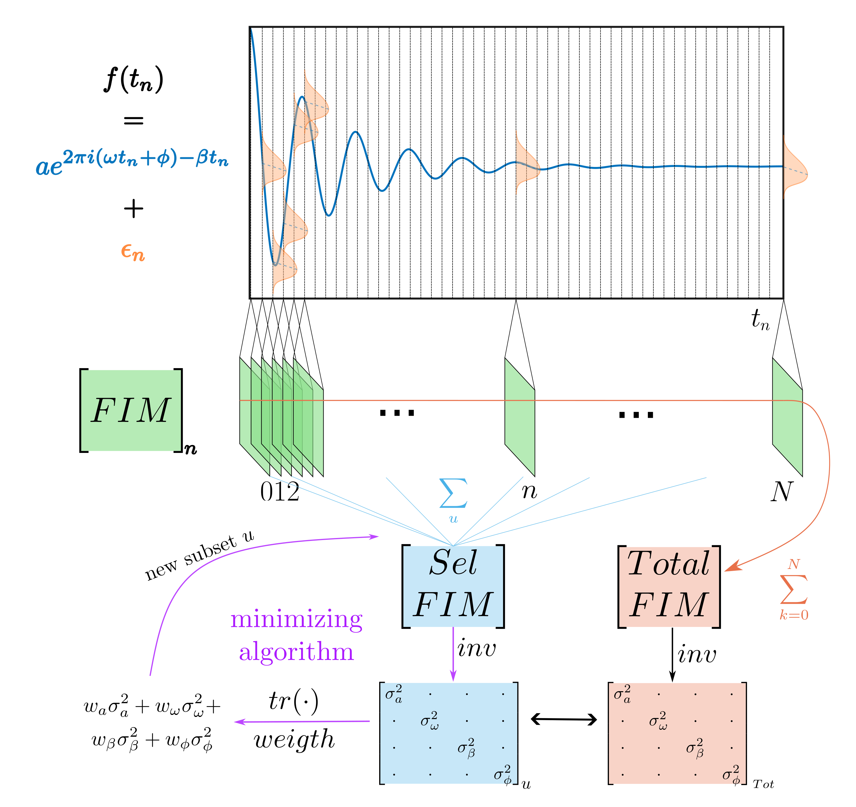
Figure 1: Scheme of the Fisher method. An assumed signal is discretized using a uniform grid respecting the Nyquist conditions. For every considered sampling point $n$, the FIM for the parameters of the signal is calculated, for that sampling point. As the Fisher information is additive, the sum of all matrices can be combined to a total FIM, which then takes into account all sampling points. The inverse of total FIM contains on the diagonal the variances of all the parameters, which correspond to a lower bound on these parameters. The same procedure can be applied on a subset of sampling points $u$, in this way obtaining a lower bound on the variances of the parameters that could be obtained by acquiring only data on the reduced subset. The variances of the total ($Tot$) and selected ($u$) sampling schemes can be compared to check the goodness of the selected subset. The minimization of the weighted variances is used to find the best subset $u$.

It is worth noting that one may in this way determine the best subset for any percentage of data in the subset (with the constraint that the FIM has to be invertible), for any noise level, as well as for various functions.

To give some examples, we examine a (real-valued) decaying exponential

$$s(t)=ae^{-\beta t}$$ (6)

In this case, the unknown parameters are $\theta=[\begin{array}[]{cc}a&\beta\end{array}]^{T}$, i.e., the observables one would want to extract from the measurement (e.g. lifetime measurements, kinetics constant). The application of the FI method [21] will find the best coordinates where to sample to be able to best estimate $a$ and $\beta$. For simplicity, we will in this example weight the two parameters equally. The assumed signal has to be first discretized along the time axis, which is here done using $N=251$ points (for instance from time 0 to 100 fs, with 0.4 fs step). Then, the algorithm is applied for a different amount of points in the subset $N_{u}$, finding at each time the best subset $u$. The sum of the selected subset depicts a histogram that can be related to an "information density" along the time axis, i.e., the more a coordinate is selected in different minimizations, the more information it carries. As can be seen in Figure 2(a), for a single real-valued exponential decay, the information, displayed as a background heat map, primarily depends on $\beta$, with most of the information being distributed in 2 regions, around $t=0$ and $t\approx 1.3/\beta$. In other words, in an experiment with noise that can be well modeled as being Gaussian, the best sampling scheme to ensure minimum variance of estimated $a$ and $\beta$ is around these two time regions. From a logical point of view, one can imagine how collecting data only around $t=0$ could lower the variance of $a$, but, at the same time, it will lead to a significant uncertainty on the resulting estimate of the decay constant, because without having data points at longer $t$, no information about how the signal has decayed is available.

Passing from a single function signal to a multi-function one, such that

$$s(t)=\sum_{k=1}^{d}a_{k}e^{-\beta_{k}t}$$ (7)

where $d$ denotes the number of decaying signal components, the logic connected to the information density pattern is more involved and less easily overseen, yet the approach is the same. The more complex pattern for this case is shown in Figure 2(b).

It is worth noting that the number of unknowns, and therefore the dimension of the resulting FIM, scales linearly with the number of components, $d$. This will also then increase the computational complexity of forming the CRLB as the cost of inverting the resulting FIM is increasing with the cube of the number of unknown parameters. If the signal is oscillating, it is instead more convenient to describe it as a complex decaying exponential, as in the introductory example, that expresses both these behaviors, i.e.,

$$s(t)=ae^{2\pi i(\omega t+\phi)-\beta t}$$ (8)

with parameters vector $\theta=[a,\omega,\beta,\phi]$. If a given parameter, say the amplitude $a$, is the component of primary interest, one may then select a weighting vector

$${\bf w}=[\begin{array}[]{cccc}w_{a}&w_{\omega}&w_{\phi}&w_{\beta}\end{array}]^{T}=[\begin{array}[]{cccc}1&0&0&0\end{array}]^{T}$$ (11)

In Figure 2(c), it is shown how the information density varies as one parameter per time is taken into account. It is worth noting that by considering only $\beta$ or $\omega$, the optimal information is to be found in the same sampling points, as is also the case if considering only $a$ or $\phi$. This similarity is not really surprising as, in this function, the gradients over either of these parameters are the same. Indeed, as seen in (Fisher Information in Time-Domain Spectroscopy), both $\beta$ and $\omega$ scale with $t$, whereas $a$ and $\phi$ do not. More surprising is that, as shown in Figure 2(d), the information density does not depend noticeably on the frequency but only on the decay rate, analogously to the simple non-oscillating exponentials in Figure 2(a). This conclusion holds as long as we consider complex-valued signals. However, in most spectroscopies, the acquisition is of real-valued data, such that $s(t)=ae^{-\beta t}cos(2\pi(\omega t+\phi))$. The difference, shown in Figure 2(e), in purple and light blu-green traces, can be easily explained by thinking at a node point: the sampling of a node of a real-valued signal will carry information about the frequency and phase, but no information about the amplitude or the decay rate, while in a complex-valued signal, it is independent, as a node in the real part corresponds to a maximum (or minimum) in the imaginary equivalent. It should be stressed that it is possible to apply the methodology directly considering real-valued data function, however, this will require having a priori knowledge about the frequency and phase of the signal. To reduce the influence of the considered subset on frequencies and phases, it is possible to use a complex-valued assumption function to retrieve the subset and apply a non-uniform Hilbert transform on collected data. If $N_{u}$ is not too small, this method works fine.

In Figure 2(e) also other typical spectroscopic functions are shown, together with the related information density. Here, the shown Gaussian or Voigt lineshapes have the forms

$$s_{G}(t) =ae^{2\pi i(\omega t+\phi)-\Delta t^{2}}$$ (12)

$$s_{V}(t) =ae^{2\pi i(\omega t+\phi)-\beta t-\Delta t^{2}}$$ (13)

for which the parameters vectors will be $\theta_{G}=[a,\omega,\Delta,\phi]$ and $\theta_{V}=[a,\omega,\beta,\Delta,\phi]$, respectively. It is worth noticing that, for the Voigt profile, a second region of information density appears at $t>0$. This happens because having equally weighted parameter variances, the algorithm has to retrieve information on both the linear ($\beta$) and quadratic ($\Delta$) terms of the decay, requiring two different regions to properly distinguish them. This is equivalent, in the fitting algorithms, to the requirement of having at least the same number of data points as compared to the number of parameters. Another example of foreknowledge for many spectroscopies is represented by the laser pulse or an instrument response function (IRF). In many experiments, the acquired signal is convoluted with these instrumental functions, which are usually very well characterized. The assumed signal could then be written, for the complex-valued exponential response, as

$$s(t)=pulse(t)*ae^{2\pi i(\omega t+\phi)-\beta t}\quad or\quad IRF(t)*ae^{2\pi i(\omega t+\phi)-\beta t}$$ (14)

Since everything is known from each pulse or IRF, the parameters will for this case still be $\theta=[a,\beta,\omega,\phi]$. If the pulse envelope width (duration) is not negligible, the information concerning the decay constant will move at longer times, as illustrated in Figure 2. This happens because the part of the signal that contains most of the information about the response moves at the edge of the convolution, whereas the initial part is mostly characterized by the pulse or the IRF. Collecting data in the initial part is equivalent to retrieving information mostly about the pulse (or IRF). If the latter is known, this would constitute redundant information, and there is no need to measure this.

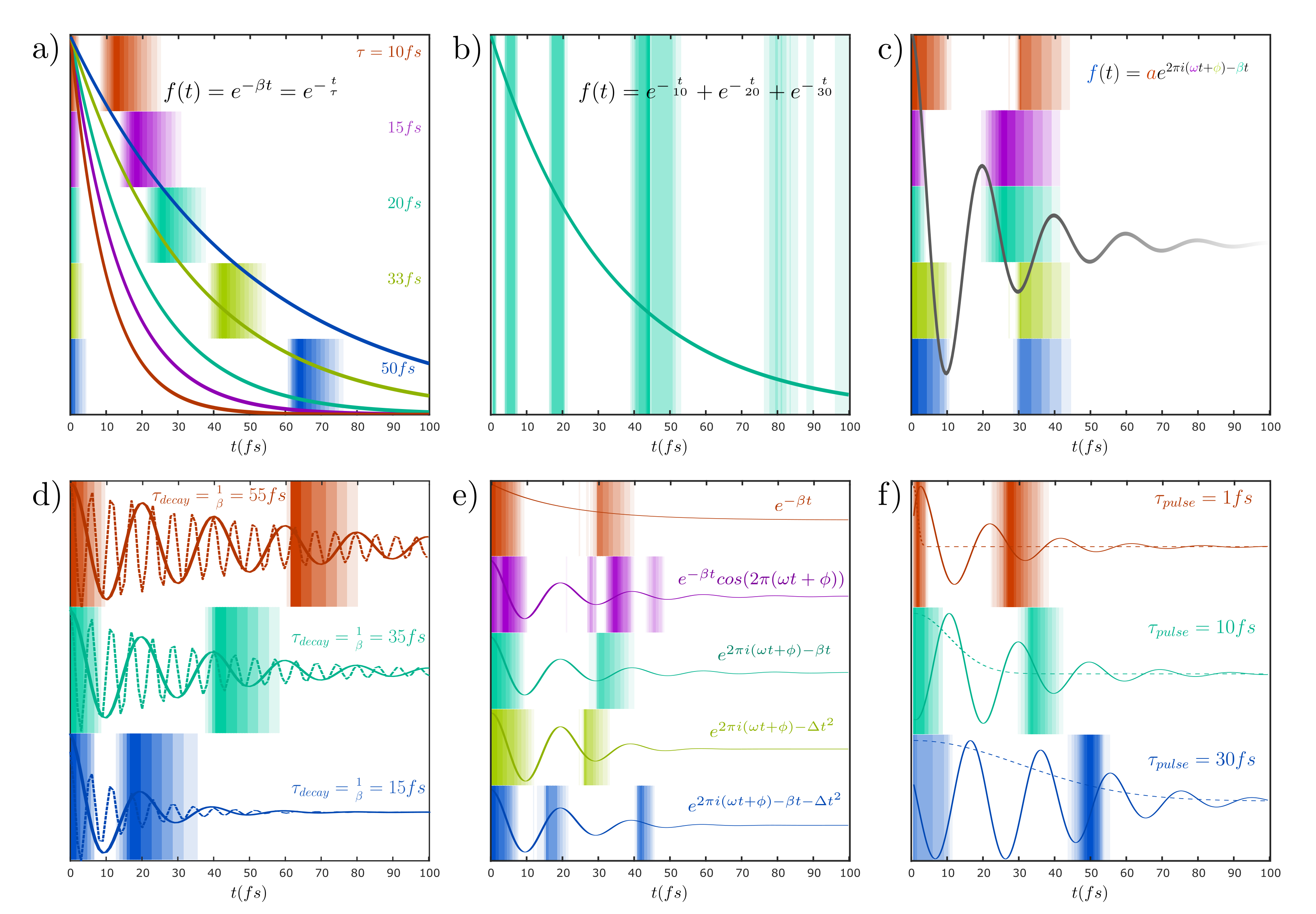
Figure 2: In this figure, the "density of information" is shown as background intensity color, formed as the sum over the selected sampling points considering different amounts of data, so that the more intense color corresponds to sampling points selected more times, using more and more samples. In a) is displayed the information about $a$ and $\beta$ for a simple real-valued exponential, as a function of $\beta$ or $\tau$. As may be seen, the information is concentrated at 0 and at $\approx 1.3\tau$. When more exponentials are summed, the selected points pattern becomes more complicated, as shown in b). In c), a complex-valued exponential function is shown, with information densities related to specific parameters (minimizing the variance of only one parameter each time). In d), trends of information densities, for varying decay constant and frequency are shown. Surprisingly, the frequency does not influence the location of information significantly, which is governed primarily by $\beta$. In e), the information density of an exponential convoluted with a Gaussian pulse with increasing width (and frequency centered at the exponential frequency) is shown, whereas f) shows a comparison of the information density of different kinds of functions (but with the same frequency and similar decay time) exponential. It is worth noting that the Voigt function adds a further density region, required to retrieve both the decay parameters $\beta$ and $\Delta$. The use of a real-valued decaying sinusoidal function gives rise to a more complicated information pattern, which will depend on both the frequency and the phase.

The minimization of the variance of an observable carries many advantages with it, beyond the pure reduction of uncertainty in itself. A concrete application that can profit from minimized variance is the classification of different spectra with a reduced amount of required collected data. To better show the potential of the technique, we examine a classification experiment of 2 type of molecules, which are to be distinguished using a FT-Raman experiment. In the experiment, the molecules’ spectra are generated (in the frequency domain) using five Lorentzian peaks with random amplitudes, frequencies, and linewidths, as shown in Figure 3(a). The time domain spectra are recreated using a Fourier transform, where only the real part is kept (to describe a real experiment), as shown in Figure 3(b). The time axis has been scaled with a range from 0 to 1000 fs, with 0.4 fs time step (2501 data points), such that it complies with the Nyquist limits of a hypothetical HeNe laser generated stokes Raman signal. We compare three different sampling methods: other than the proposed Fisher method, we employ a (uniformly distributed) random selection as well as a Poisson gap sampling scheme. The former comprises an example of so-called compressive sampling. The latter uses a denser-to-sparser sampling scheme and has already been demonstrated to be advantageous for free induction decay data [15]). The selected points are identified by the markers shown in Figure 3(b). To distinguish the two molecules, it is possible to focus on selected or all of the parameters detailing the peaks, amplitudes, and/or linewidths. For simplicity and to better display the results, we chose the amplitudes of only 2 spectral peaks in the 2 types of molecules (shown using dashed vertical lines in Figure 3(a)). For the Fisher method, the assumed signal model is represented by the sum of all the 10 Lorentzians, although the classification, again for simplicity, has only been formed using two dominant peaks that do not overlap in frequency, one for each molecule. The weight function has been chosen to minimize the variance of the amplitudes of these two peaks, in order to accurately be able to determine these. Once the data are extracted from the full dataset for each sampling method, the amplitudes are retrieved by least square minimization of the two oscillating functions

$$f(t_{s})=a_{1}exp(i\omega_{1}t_{s})+a_{2}exp(i\omega_{2}t_{s})$$ (15)

where $t_{s}$ are the selected time points for each selection method and $\omega_{1}$, $\omega_{2}$ are the frequency of the two peaks. It may be noted that the minimization function could also take into account, for instance, the decay rates for a better fitting. We proceed to form Monte-Carlo simulations, with a randomly drawn noise in each simulation, by randomly selecting one of the two considered molecules, adding Gaussian noise (ranging from -40 to 10 dB of SNR), retrieving the selected coordinates, and estimating the complex amplitudes $a_{1}$ and $a_{2}$. This procedure is repeated for different fractions of used data (ranging from 1 to 12 %, i.e., using only 25 to 300 out of the total 2501 data points). The absolute amplitudes of the 2 peaks for each iteration $[\lvert a_{1}\rvert,\lvert a_{2}\rvert]$ are displayed in scatter plots in Figure 3(c). For all noise and data percentage levels, the classification is performed using linear discriminant analysis. This supervised machine learning method simply finds the best line that separates the two molecules’ ensembles in the $[a_{1},a_{2}]$ space. As the accuracy of the classification relies on how many times the retrieved amplitude sets fall into the correct part of the line, a lower variance of amplitudes will lead to less probability of failure and as a result a better classification. As can be seen in the figure, as the SNR increases, there is a reduction of the dispersion and an improvement in the accuracy of the classification for all methods, with the Fisher method clearly showing superior performance. The same results, but more in detail, can be seen in Figure 3(d), where the accuracy of the classifications of the 3 sampling methods are plotted as a function of both the SNR and the percentage of used data, showing also the difference between them in the maps on the right. As can be seen in the figure, the Fisher method offers notably improved performance over the Poisson gap sampling, and with the random sampling scheme showing, as expected, the worst performance.

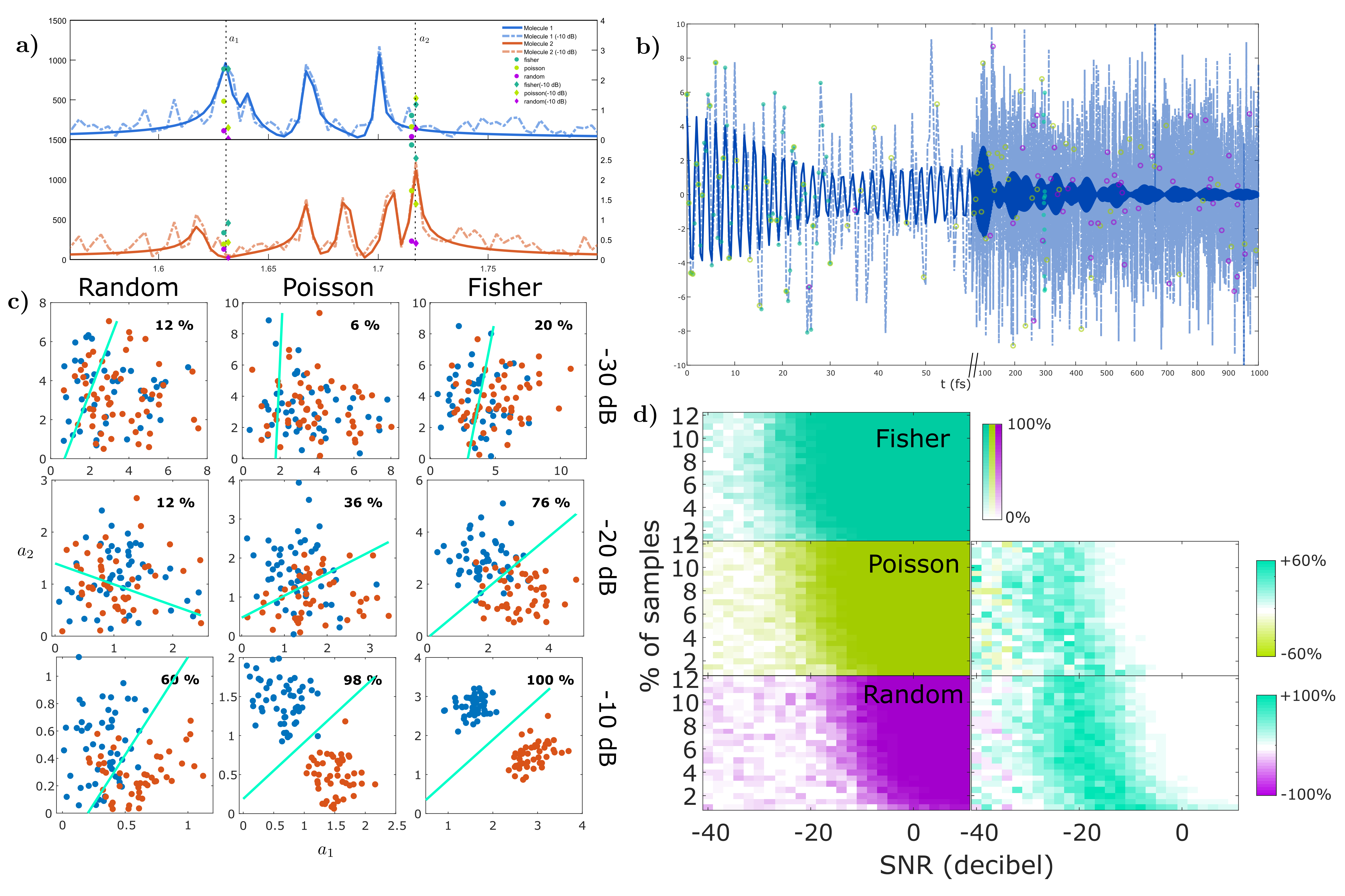
Figure 3: a) Simulated frequency domain Raman spectra of 2 molecules and b) the real part of the time-domain spectrum of molecule 1. The dashed lines identify the noisy spectra with added Gaussian noise, with SNR=10. The vertical lines identify the coordinates selected for the classification, selected as these peaks do not overlap with the peaks in the other molecule. The colored dots in a) identify the amplitudes of the least square minimization using 2 complex exponentials, with peak coordinates frequencies, on the selected datasets being shown in b), where the colors label the Fisher-, Poisson- and random-selected samples. c) shows the distribution of the fitted amplitudes for different SNR for randomly generated data sets using 100 Monte-Carlo simulations. It is worth noting the lower variance of the amplitudes for the Fisher method, for every SNR. This in turn leads to better performance when performing linear discriminant analysis for the classification. In d), the increased accuracy for the Fisher subset is compared to the Poisson and random sampling schemes, as a function of SNR and percentage of data collected.

The sampling optimization is not limited to one dimension but can be extended to multidimensional spectroscopies like 2DIR or 2DES, or in magnetic spectroscopies or multidimensional NMR. To illustrate this, we present an example of smart sampling in 2DES experiments. 2DES is a spectroscopy that aims to collect the ultrafast non-linear response from the sample by means of interaction between the sample and ultrafast pulses. Different 2DES configurations and geometries are in use [27], each with its pros and cons. Especially the collinear beam geometry is drawing attention as it allows to detect functional signal, and combine the 2DES with local detection and imaging. To exploit the advantages of the collinear beam geometry, it is necessary to change from the coherent heterodyne detection with an excited-state population-based detection, such as fluorescence [28], current [29, 30] or photo-electron detection [31]. Population detection requires a different approach to retrieve the components of the non-linear signals [32]. First, it is necessary to scan the third delay of a fourth pulse instead of the usual two delays between the three pulses of the BOXCAR 2DES. Then, to retrieve the different components of the non-linear signals, it is also necessary to perform a phase cycling [33], which dramatically increases the number of required acquisitions. Put differently, it is necessary to have control and scan the various delays ($t_{1}$, $t_{2}$, and $t_{3}$) as well as phases ($\Delta\phi_{1}$, $\Delta\phi_{2}$, and $\Delta\phi_{3}$) between the 4 pulses. To retrieve only one full 2DES map at fixed population time, a typical number of acquisitions, assuming a rotating frame is applied, can be 15x15x3x3x3=6075 scanning points over $t_{1}$, $t_{3}$, $\Delta\phi_{1}$, $\Delta\phi_{2}$, and $\Delta\phi_{3}$, respectively. To overcome the resulting huge amount of acquisitions, beyond fast shot-by-shot detections [28], many groups have proposed and exploited compressed sensing methods with the aim of retrieving the signal with a reduced number of acquisitions [19, 34, 35]. Noticeable is the approach of the Brixner group that exploits a basis change from time coordinates to a von Neumann basis [36]. However, the goal of all these methods is to reconstruct the signal. On the contrary, our approach instead reduces the number of acquisitions focusing on reducing the variance of the observables, and the proper reconstruction of the signal is just a consequence. Here, we present an example with simulated population-detected 2DES data. Even if the non-linear signal depends on the Hamiltonian of the system and has complex dependencies on the different delays and phases, it can often be well approximated as a sum of simpler functions, at least along the time axes $t_{1}$ and $t_{3}$, where coherences between the ground and excited state evolve as decaying oscillations. Here, we apply Lorentzian, Gaussian, and Voigt two-dimensional (2D) functions or the sum of them, i.e.,

$$\begin{split}L(t_{1},t_{3})&=ae^{2\pi i(\omega_{1}t_{1}\pm\omega_{3}t_{3}\pm\phi_{13})-\beta_{3}t_{3}-\beta_{3}t_{3}}\\ G(t_{1},t_{3})&=ae^{2\pi i(\omega_{1}t_{1}\pm\omega_{3}t_{3}\pm\phi_{13})-\Delta_{1}t_{1}^{2}-\Delta_{3}t_{3}^{2}}\\ V(t_{1},t_{3})&=ae^{2\pi i(\omega_{1}t_{1}\pm\omega_{3}t_{3}\pm\phi_{13})-\beta_{1}t_{1}-\Delta_{1}t_{1}^{2}-\beta_{3}t_{3}-\Delta_{3}t_{3}^{2}}\end{split}$$ (16)

Where $\pm$ differentiates the rephasing and non-rephasing signals, while $\beta$ and $\Delta$ are the coefficient of the linear and quadratic components, respectively. We proceed by applying the Fisher method to select the best acquisition coordinates ($t_{1},t_{3}$) to minimize the variance of the parameters of the assumed signals. In this example, we use a tentative grid in the range of 0-50 fs with a 1 fs step. Figure 4 shows the outcome of the selections for the considered cases. For the single spectral components selections, on the left part of the figure, the signal parameters are $a=1,\beta_{1,3}=0.05$ ($\tau=20$ fs), $\Delta_{1,3}=\beta_{1,3}^{2},\omega_{1}=-\omega_{3}=0.05$ fs^-1, and $\phi=0$, except for the Voigt profile $V(t_{1},t_{3})$ where $\beta$ and $\Delta$ are halved to make the decaying profile comparable with the other functions. In the first and the second rows are shown the signals along the frequency and time axes, respectively. The former was obtained through a zero-padded Fourier transform. From the third row on, the graphs identify the selection of the most "informative coordinates". The third is when the weights of all the parameters are equally balanced, the fourth is with the focus on the decaying parameters, and the fifth is on frequency. The last row shows the information distribution obtained after 200 Monte-Carlo simulations, where the decaying parameters of the signal models are randomly chosen within a "reasonable" range ($0.01$ fs${}^{-1}<\beta<0.1$ fs^-1). On the right column, the same approach and graphs are shown, but two more spectral components have been added, to make the final frequency domain 2DES map resemble typical experimental case, with slightly different decay parameters and frequency positions.

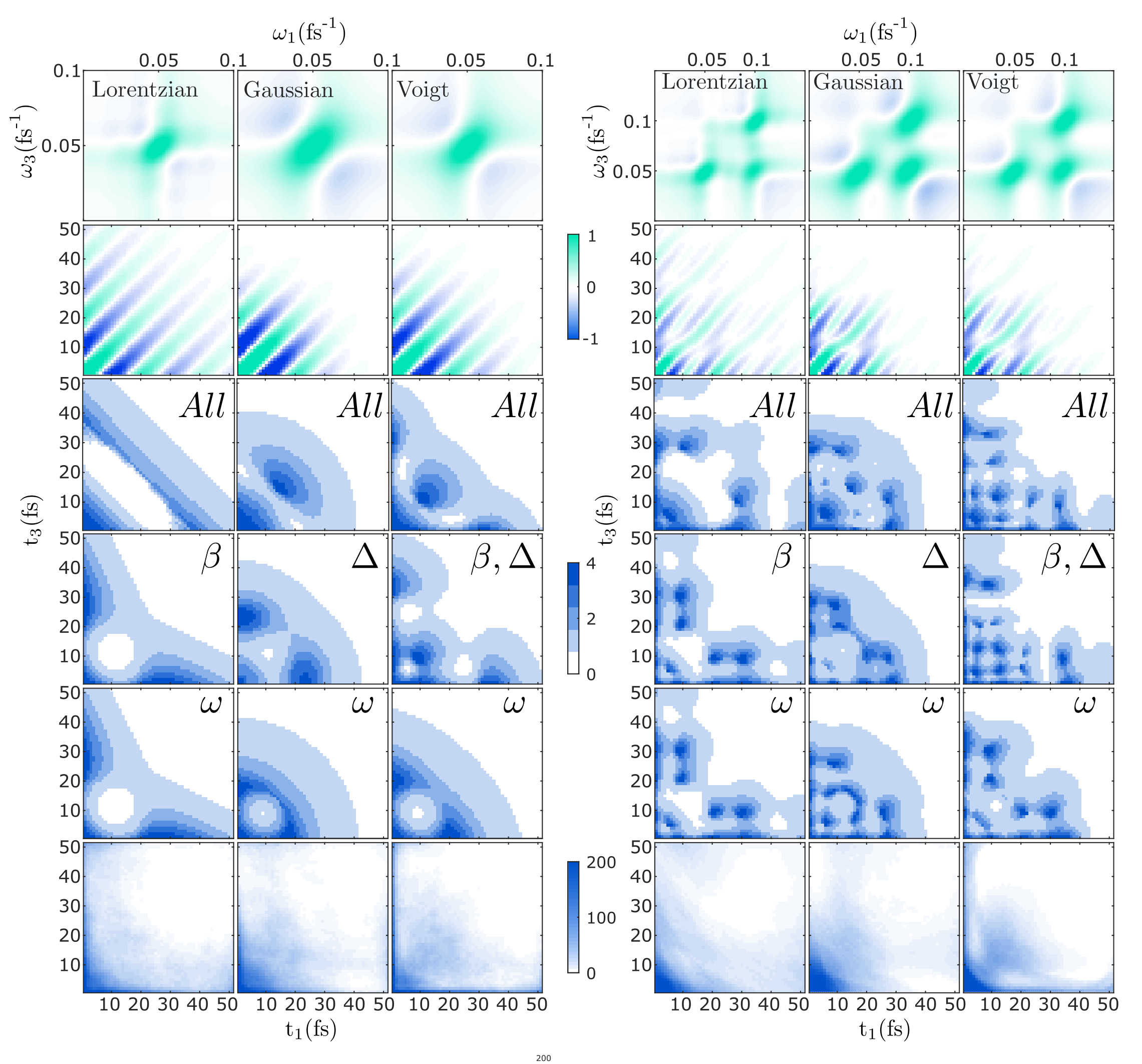
Figure 4: Distribution of information in time-domain 2D spectra using different 2D lineshapes. On the left, the figures only contain one spectral component, whereas, on the right, spectra that resemble typical experimental 2D spectra with 3 spectral components are shown. The first and the second rows display frequency- and time-domain 2D lineshapes, respectively. The third one shows information distribution when all parameters has same weight. The fourth and fifth when the minimization is focused on temporal or frequency parameters, respectively. The last row shows the Monte-Carlo-averaged information distribution. It is worth noting that in almost all cases, the information is distributed mainly in the 2D zones close to the axes.

Assuming phase cycling or modulation, the acquired data is complex-valued. As for the 1D case, the results are not influenced by the frequency, rephasing and non-rephasing maps have identical information densities, differing between each other only for frequency sign. In Figure 4, only rephasing data are shown. From these simulations, one may conclude that the information concerning the observables is distributed mainly at short times, as expected since the signal is higher, and close to axes, i.e., at short $t_{3}$ when $t_{1}$ is long, and vice versa. This is not surprising as, for example, in order to retrieve $\beta_{1}$, it is better to examine the evolution of the signal along $t_{1}$ at small $t_{3}$ where the SNR is higher. The exception is represented by the Voigt profile function, which has a relevant amount of information also along the diagonal, as the signal is much more sensitive to changes in $\beta$ and $\Delta$ (they are less covariant), and the diagonal is then the best place to select samples aiming to minimize their variances simultaneously. If the weight of one of the two parameters is set to 0, the information along the diagonal vanishes.

In this work, we presented some examples of the application of the Fisher information in spectroscopy. We limited the methodology to single-value parameters for the assumed signal model, but the method is applicable to models described using ranges or distributions of parameters, relaxing the required foreknowledge [21]. In the above presentation, we have mainly assumed that the additive noise may be well modeled as being Gaussian, although the methodology does not impose such a restriction as such. Other noise distributions may also be considered. A practical example is the Poisson (shot) noise, almost always present in photon detection, even if it is often convoluted with other noise sources, often allowing the overall noise to be well modeled as being Gaussian. In case there are no other noise sources, the noise would not be constant along the time coordinate, but it will depend directly on the amplitude of the signal itself. As the here used optimization technique minimizing the CRLB [21] employs approximations assuming that the noise is well modeled as being Gaussian, these steps would need to be reformulated if considering other noise distributions, although the overall methodology would remain unchanged. It is further worth noting that the methodology may be applied iteratively, thereby allowing for the optimization of additional time points in real-time acquisitions [37]. After the acquisition of a first subset and subsequent initial estimation of the parameters, the algorithm will then determine the best next coordinate(s) that have to be measured to reduce the variance of the desired parameters. In principle, this leads to the acquisition of new sampling points, but also to averaging the previously acquired ones. The method is powerful for classification; here, more efficient classifications are achieved by including further parameters per molecule; the method can be extended to allow for more molecules/spectra. Moreover, more complex classification analyses may be implemented using the acquired data, for instance employing higher-order discriminant or neuronal networks. Finally, our approach has been shown to produce a sampling scheme for collinear 2DES spectroscopy denser along the axes in contrast with more homogeneously sparse sampling reported in the literature [36]. This is because our approach is observable-oriented and does not directly aim to reconstruct the signal.

Aknowledgment

The authors would like to acknowledge helpful discussions with Prof. Tonu Pullerits, Mr Edvin Sanden, and Mr. Pontus Walan.

References

- [1] C. Berthomieu and R. Hienerwadel, “Fourier transform infrared (FTIR) spectroscopy,” Photosynthesis Research, vol. 101, no. 2-3, pp. 157–170, 9 2009. [Online]. Available: https://link.springer.com/article/10.1007/s11120-009-9439-x
- [2] C. Fernandez, R. Bhargava, S. M. Hewitt, I. W. Levin, . E. Wolf, . R. Hillenbrand, . F. Huth, A. Govyadinov, S. Amarie, W. Nuansing, F. Keilmann, R. Hillenbrand, . S. Poly, M. Goikoetxea, and P. Lasch, “Compressed sensing FTIR nano-spectroscopy and nano-imaging,” Optics Express, Vol. 26, Issue 14, pp. 18115-18124, vol. 26, no. 14, pp. 18 115–18 124, 7 2018. [Online]. Available: https://opg.optica.org/viewmedia.cfm?uri=oe-26-14-18115&seq=0&html=truehttps://opg.optica.org/abstract.cfm?uri=oe-26-14-18115https://opg.optica.org/oe/abstract.cfm?uri=oe-26-14-18115
- [3] T. Hirschfeld and B. Chase, “FT-Raman Spectroscopy: Development and Justification,” Applied Spectroscopy, vol. 40, no. 2, pp. 133–137, 2 1986. [Online]. Available: http://journals.sagepub.com/doi/10.1366/0003702864509538
- [4] D. Naumann, “FT-INFRARED AND FT-RAMAN SPECTROSCOPY IN BIOMEDICAL RESEARCH,” Applied Spectroscopy Reviews, vol. 36, no. 2-3, pp. 239–298, 6 2001. [Online]. Available: http://www.tandfonline.com/doi/abs/10.1081/ASR-100106157
- [5] D. P. Millar, “Time-resolved fluorescence spectroscopy,” Current Opinion in Structural Biology, vol. 6, no. 5, pp. 637–642, 10 1996.
- [6] K. Suhling, P. M. French, and D. Phillips, “Time-resolved fluorescence microscopy,” Photochemical & Photobiological Sciences, vol. 4, no. 1, pp. 13–22, 12 2005. [Online]. Available: https://pubs.rsc.org/en/content/articlehtml/2005/pp/b412924phttps://pubs.rsc.org/en/content/articlelanding/2005/pp/b412924p
- [7] C. Biskup and T. Gensch, Fluorescence Lifetime Spectroscopy and Imaging. CRC Press, 7 2014. [Online]. Available: https://www.taylorfrancis.com/books/9781439861684
- [8] A. L. Whittock, T. T. Abiola, and V. G. Stavros, “A Perspective on Femtosecond Pump-Probe Spectroscopy in the Development of Future Sunscreens,” Journal of Physical Chemistry A, vol. 126, no. 15, pp. 2299–2308, 4 2022. [Online]. Available: https://pubs.acs.org/doi/full/10.1021/acs.jpca.2c01000
- [9] M. Fushitani, “Applications of pump-probe spectroscopy,” Annual Reports Section ’C’ (Physical Chemistry), vol. 104, no. 0, pp. 272–297, 6 2008. [Online]. Available: https://pubs.rsc.org/en/content/articlehtml/2008/pc/b703983mhttps://pubs.rsc.org/en/content/articlelanding/2008/pc/b703983m
- [10] M. D. Fayer, “Vibrational echo chemical exchange spectroscopy,” Ultrafast Infrared Vibrational Spectroscopy, pp. 1–33, 1 2013. [Online]. Available: https://www.taylorfrancis.com/books/mono/10.1201/b13972/ultrafast-infrared-vibrational-spectroscopy-michael-fayer
- [11] M. Khalil, N. Demirdöven, and A. Tokmakoff, “Coherent 2D IR Spectroscopy: Molecular Structure and Dynamics in Solution,” The Journal of Physical Chemistry A, vol. 107, no. 27, pp. 5258–5279, 7 2003. [Online]. Available: https://pubs.acs.org/doi/10.1021/jp0219247
- [12] A. Gelzinis, R. Augulis, V. Butkus, B. Robert, and L. Valkunas, “Two-dimensional spectroscopy for non-specialists,” Biochimica et Biophysica Acta (BBA) - Bioenergetics, vol. 1860, no. 4, pp. 271–285, 4 2019.
- [13] E. Collini, “2D Electronic Spectroscopic Techniques for Quantum Technology Applications,” The Journal of Physical Chemistry C, vol. 125, no. 24, pp. 13 096–13 108, 6 2021. [Online]. Available: https://pubs.acs.org/doi/10.1021/acs.jpcc.1c02693
- [14] S. G. Hyberts, K. Takeuchi, and G. Wagner, “Poisson-Gap Sampling and Forward Maximum Entropy Reconstruction for Enhancing the Resolution and Sensitivity of Protein NMR Data,” Journal of the American Chemical Society, vol. 132, no. 7, pp. 2145–2147, 2 2010.
- [15] P. Kasprzak, M. Urbańczyk, and K. Kazimierczuk, “Clustered sparsity and Poisson-gap sampling,” Journal of Biomolecular NMR, vol. 75, no. 10-12, pp. 401–416, 12 2021. [Online]. Available: https://link.springer.com/article/10.1007/s10858-021-00385-7
- [16] S. Bagchi and S. K. Mitra, The Nonuniform Discrete Fourier Transform and Its Applications in Signal Processing. Boston, MA: Springer US, 1999. [Online]. Available: http://link.springer.com/10.1007/978-1-4615-4925-3
- [17] A. J. W. Duijndam and M. A. Schonewille, “Nonuniform fast Fourier transform,” GEOPHYSICS, vol. 64, no. 2, pp. 539–551, 3 1999. [Online]. Available: https://library.seg.org/doi/10.1190/1.1444560
- [18] E. Andries and S. Martin, “Sparse Methods in Spectroscopy: An Introduction, Overview, and Perspective,” Applied Spectroscopy, vol. 67, no. 6, pp. 579–593, 6 2013. [Online]. Available: http://journals.sagepub.com/doi/10.1366/13-07021
- [19] Z. Wang, S. Lei, K. J. Karki, A. Jakobsson, and T. Pullerits, “Compressed Sensing for Reconstructing Coherent Multidimensional Spectra,” The Journal of Physical Chemistry A, vol. 124, no. 9, pp. 1861–1866, 3 2020. [Online]. Available: https://pubs.acs.org/doi/10.1021/acs.jpca.9b11681
- [20] G. Carlström, F. Elvander, J. Swärd, A. Jakobsson, and M. Akke, “Rapid nmr relaxation measurements using optimal nonuniform sampling of multidimensional accordion data analyzed by a sparse reconstruction method,” Journal of Physical Chemistry A, vol. 123, no. 27, pp. 5718–5723, 6 2019. [Online]. Available: https://pubs.acs.org/doi/full/10.1021/acs.jpca.9b04152
- [21] J. Swärd, F. Elvander, and A. Jakobsson, “Designing sampling schemes for multi-dimensional data,” Signal Processing, vol. 150, pp. 1–10, 9 2018. [Online]. Available: https://linkinghub.elsevier.com/retrieve/pii/S0165168418301099
- [22] J. Swärd, S. I. Adalbjörnsson, and A. Jakobsson, “High resolution sparse estimation of exponentially decaying N-dimensional signals,” Signal Processing, vol. 128, pp. 309–317, 11 2016.
- [23] D. Potts, M. Tasche, and T. Volkmer, “Efficient Spectral Estimation by MUSIC and ESPRIT with Application to Sparse FFT,” Frontiers in Applied Mathematics and Statistics, vol. 2, p. 1, 2 2016.
- [24] A. Elsener and S. van de Geer, “Sparse spectral estimation with missing and corrupted measurements,” Stat, vol. 8, no. 1, p. e229, 1 2019. [Online]. Available: https://onlinelibrary.wiley.com/doi/full/10.1002/sta4.229https://onlinelibrary.wiley.com/doi/abs/10.1002/sta4.229https://onlinelibrary.wiley.com/doi/10.1002/sta4.229
- [25] S. M. Kay, Fundamentals of Statistical Processing: Estimation Theory. Upper Saddle River, New Jersey: Prentice Hall, 1993, vol. 1. [Online]. Available: https://www.pearson.com/en-us/subject-catalog/p/fundamentals-of-statistical-processing-estimation-theory-volume-1/P200000009271/9780133457117
- [26] W. Limmun, J. J. Borkowski, and B. Chomtee, “Weighted A-optimality criterion for generating robust mixture designs,” Computers & Industrial Engineering, vol. 125, pp. 348–356, 11 2018.
- [27] F. D. Fuller and J. P. Ogilvie, “Experimental Implementations of Two-Dimensional Fourier Transform Electronic Spectroscopy,” Annual Review of Physical Chemistry, vol. 66, no. 1, pp. 667–690, 4 2015. [Online]. Available: https://www.annualreviews.org/doi/10.1146/annurev-physchem-040513-103623
- [28] S. Draeger, S. Roeding, and T. Brixner, “Rapid-scan coherent 2D fluorescence spectroscopy,” Optics Express, vol. 25, no. 4, p. 3259, 2 2017. [Online]. Available: https://opg.optica.org/abstract.cfm?URI=oe-25-4-3259
- [29] L. Bolzonello, F. Bernal-Texca, L. G. Gerling, J. Ockova, E. Collini, J. Martorell, and N. F. Van Hulst, “Photocurrent-Detected 2D Electronic Spectroscopy Reveals Ultrafast Hole Transfer in Operating PM6/Y6 Organic Solar Cells,” Journal of Physical Chemistry Letters, vol. 12, no. 16, pp. 3983–3988, 2021.
- [30] K. J. Karki, J. R. Widom, J. Seibt, I. Moody, M. C. Lonergan, T. Pullerits, and A. H. Marcus, “Coherent two-dimensional photocurrent spectroscopy in a PbS quantum dot photocell,” Nature Communications, vol. 5, no. 1, p. 5869, 12 2014. [Online]. Available: http://www.nature.com/articles/ncomms6869
- [31] M. Aeschlimann, T. Brixner, A. Fischer, C. Kramer, P. Melchior, W. Pfeiffer, C. Schneider, C. Strüber, P. Tuchscherer, and D. V. Voronine, “Coherent Two-Dimensional Nanoscopy,” Science, vol. 333, pp. 1723–1727, 2011.
- [32] P. Malý, J. Lüttig, S. Mueller, M. H. Schreck, C. Lambert, and T. Brixner, “Coherently and fluorescence-detected two-dimensional electronic spectroscopy: direct comparison on squaraine dimers,” Physical Chemistry Chemical Physics, vol. 22, no. 37, pp. 21 222–21 237, 9 2020. [Online]. Available: http://xlink.rsc.org/?DOI=D0CP03218B
- [33] H.-S. Tan, “Theory and phase-cycling scheme selection principles of collinear phase coherent multi-dimensional optical spectroscopy,” The Journal of Chemical Physics, vol. 129, no. 12, p. 124501, 9 2008. [Online]. Available: http://aip.scitation.org/doi/10.1063/1.2978381
- [34] A. P. Spencer, B. Spokoyny, S. Ray, F. Sarvari, and E. Harel, “Mapping multidimensional electronic structure and ultrafast dynamics with single-element detection and compressive sensing,” Nature Communications, vol. 7, no. 1, p. 10434, 4 2016. [Online]. Available: http://www.nature.com/articles/ncomms10434
- [35] J. N. Sanders, S. K. Saikin, S. Mostame, X. Andrade, J. R. Widom, A. H. Marcus, and A. Aspuru-Guzik, “Compressed Sensing for Multidimensional Spectroscopy Experiments,” The Journal of Physical Chemistry Letters, vol. 3, no. 18, pp. 2697–2702, 9 2012. [Online]. Available: https://pubs.acs.org/doi/10.1021/jz300988p
- [36] S. Roeding, N. Klimovich, and T. Brixner, “Optimizing sparse sampling for 2D electronic spectroscopy,” Journal of Chemical Physics, vol. 146, no. 8, 2017. [Online]. Available: http://dx.doi.org/10.1063/1.4976309
- [37] F. Elvander, J. Swärd, and A. Jakobsson, “An efficient solver for designing optimal sampling schemes,” ArXiv, 11 2021. [Online]. Available: http://arxiv.org/abs/2111.05579