Draft: Low Complexity Time Synchronization for Zero-padding based Waveforms

Abstract

The discussion on using zero padding (ZP) instead of a cyclic prefix (CP) for enhancing channel estimation and equalization performance is a recurring topic in waveform design for future wireless systems that high spectral efficiency and location awareness are the key factors. This is particularly true for orthogonal signals, such as orthogonal frequency-division multiplexing (OFDM). ZP-OFDM is appealing for joint communications and sensing (JCS) in 6G networks because it takes the advantage of both OFDM and pulse radar. In term of communication, ZP-OFDM compared to CP-OFDM, has higher power efficiency and lower bit error rate (BER). However, time synchronization is challenging in ZP-OFDM systems due to the lack of CP. In terms of sensing, ZP facilitates ranging methods, such as time-sum-of-arrival (TSOA). In this paper, we propose a moment-based timing offset (TO) estimator for multiple-input multiple-output (MIMO) ZP-OFDM system without the need for pilots. We then introduce the

which significantly improves the estimation accuracy of the previous estimator. We show that the proposed method asymptotically reaches the maximum likelihood (ML) estimator. Simulation results show very high probability of lock-in for the proposed estimators under various practical scenarios.

I Introduction

Orthogonal frequency-division multiplexing (OFDM) technique is widely employed in wireless communication systems, mainly due to its ability to convert a frequency-selective fading channel into a group of flat-fading sub-channels [1]. Compared to conventional single-carrier systems, OFDM offers increased robustness against multipath fading distortions since channel equalization can be easily performed in the frequency domain through a bank of one-tap multipliers [2]. Moreover, OFDM can be efficiently implemented using fast fourier transform (FFT) [3], which makes it more appealing compared to other multi-carrier modulation techniques such as filter bank multi carrier and generalised frequency division multiplexing.

Because of its advantages, OFDM is used in many IEEE standards, such as, IEEE 802.15.3a, IEEE 802.16d/e, and IEEE 802.15.4g [4, 5, 6]. In addition, OFDM combined with massive MIMO technique achieves a high data rate, making it suitable for multimedia broadcasting [7]. Moreover, many internet of things (IoT) applications such as smart buildings and vehicle-to-everything (V2X) leverage OFDM as their main communication scheme [8, 6].

OFDM, however, is susceptible to sever inter symbol interference (ISI) caused by the high selectivity of the fading channel [9]. In order to mitigate this issue, usually a guard interval with a fixed length is inserted between every two consecutive OFDM symbols. When the guard interval is the partial repetition of the transmitting data samples, this scheme is called cyclic prefix (CP)-OFDM [10]. When the guard interval is filled with zeros, the scheme is called zero-padded (ZP)-OFDM [11].

The discussion on using ZP instead of a CP for enhancing channel estimation and equalization performance is a recurring topic. This is particularly true for orthogonal signals, such as OFDM. The primary benefit of CP-OFDM over ZP-OFDM is the ease of timing offset (TO) estimation or equivalently estimating the starting point of the received samples to apply fast Fourier transform (FFT). This is referred to as time synchronization [12], and is easily carried out by using CP and its correlation with the data sequence. Despite the ease of time synchronization, CP-OFDM has some major disadvantages such as extra power transmission and a higher BER compared to ZP-OFDM [13], which are due to the transmission of CP. While ZP-OFDM does not have such drawbacks, its time synchronization or equivalently TO estimation is very difficult and complicated [14].

There are two approaches in order to estimate TO in ZP-OFDM. In the first approach, called data-aided (DA) time synchronization, a series of training sequences (pilots) are used to estimate TO. The second approach, referred to as non-data-aided (NDA) time synchronization, relies on the statistical properties of the transmitted data sequence. In the next subsection, we briefly review TO estimation methods proposed for both DA and NDA time synchronization in ZP-OFDM systems.

I-A Related work

The DA time synchronization for ZP-OFDM has been studied in the literature [15], where a highly correlated training sequence (pilot) is employed in order to increase the auto-correlation of the received signal, which is then used for estimating the TO. Such a pilot-based time synchronization algorithm can achieve reliable performance while having a reasonable complexity [15]. For NDA time synchronization in ZP-OFDM, however, a low-complexity TO estimation algorithm with an accuracy comparable to that of CP-OFDM counterparts does not exist. Existing NDA time synchronization algorithms for ZP-OFDM [16, 17] mainly detect the jumps in the energy of the signal. Such methods are heuristics that detect the point that the energy of the samples in the window drops significantly. However, jump-based techniques greatly suffer from the natural randomness of the received samples; thus, exhibit poor performance in terms of probability of lock-in, i.e. correct TO estimation. A mathematical approach towards NDA TO estimation for ZP-OFDM systems has been proposed in [14]. The authors in [14] proposed a ML TO estimator for ZP-OFDM under a frequency selective channel. However, the algorithm in [14] is highly complex which hinders its implementation for MIMO systems or even single-antenna mobile users. Moreover, the algorithm in [14] cannot be used for low signal-to-noise ratio (SNR) as the proposed expressions in the estimator yield infinity due to floating-point errors.

I-B Motivation

ZP-OFDM has several advantages compared to CP-OFDM [13]. For example, regardless of the channel nulls, it is possible to perform finite impulse response equalization in ZP-OFDM systems [13]. Moreover, channel estimation and tracking is easier in ZP-OFDM compared to CP-OFDM [13]. Finally, ZP-OFDM requires less transmission power compared to CP-OFDM, due to lack of CP, which makes it a suitable candidate for power-limited devices. However, time synchronization becomes challenging in ZP-OFDM where proposed NDA algorithms in the literature fail to achieve a high lock-in probability, or practical complexity. Hence, an accurate yet low-complexity NDA time synchronization algorithm for ZP-OFDM is needed. The goal of this paper is to fill this existing gap.

I-C Contributions

In this paper, we first propose a moment-based NDA TO estimator for MIMO OFDM. In general, moment estimators are derived via solving equations involving the theoretical moments of the received samples and their natural moment estimators [18]. In this paper, we choose $n=2$ in order to keep the complexity of the estimator very low. Later, we propose a weighted version of the moment estimator to further improve the the probability of lock-in. The contribution of the paper is summarized as follows

• an NDA TO estimator based on method of moments (MOM) for MIMO ZP-OFDM systems in doubly selective channels is proposed. This algorithm

  • achieves high lock-in probability,

  • has significantly lower complexity compared to [14]; thus, it can be employed in MIMO and even massive-MIMO systems.

  • is suitable for deployment in very low SNRs in contrast to [14] and TM,

• a weighted moment-based NDA TO estimator for MIMO ZP-OFDM systems in highly selective channels is proposed. This algorithm

  • has all the benefits of the first estimator while significantly improving its lock-in probability

This paper is organized as follows. The main ideas, the proposed estimators, and the complexity of the estimators are presented in Section LABEL:sec:_ml_estimation. Simulation results and conclusions are given in Sections IV and V, respectively.

Notations: Column vectors are denoted by bold lower case letters. Random variables are indicated by uppercase letters. Matrices are denoted by bold uppercase letters. Conjugate, absolute value, transpose, and the expected value are indicated by $(\cdot)^{*}$, $|\cdot|$, $(\cdot)^{\rm{T}}$, and $\mathbb{E}\{\cdot\}$, respectively. Floor function is denoted by $\lfloor\cdot\rfloor$. Brackets, e.g. ${\bf a}[k]$, are used for discrete indexing of a vector ${\bf a}$. Natural estimator of an observation sample is defined as

$$\mathbb{E}\{\lvert x[i]\rvert^{n}\}=\frac{1}{m}\sum_{i=1}^{m}\lvert x[i]\rvert^{n}.$$

I-D System model

We consider a MIMO-OFDM wireless system with $m_{\rm{t}}$ and $m_{\rm{r}}$ transmit and receive antennas, respectively. This system uses ZP-OFDM technique for JCAS over a frequency selective Rayleigh fading channel. Let $\{x^{(n,k)}_{i}\}_{k=0}^{n_{\rm{x}}-1}$ with $\mathbb{E}\{|x^{(n,k)}_{i}|^{2}\}=\sigma^{2}_{\rm{x}}$, denote the $n_{\rm{x}}$ complex data samples from the $n$-th OFDM block to be transmitted from the $i$-th transmit antenna. The corresponding OFDM signal can be expressed as

$$x^{(n)}_{i}(t)=\sum_{k=0}^{n_{{\rm{x}}-1}}x^{(n,k)}_{i}e^{\frac{j2\pi kt}{T_{\rm{x}}}}\,\,\,\,\,\,\,\,\,\,\ 0\leq t\leq T_{\rm{x}},$$ (1)

where $T_{\rm{x}}$ denotes the duration of the data signal. By adding a zero-padding guard interval of length $T_{{\rm{z}}}$ to (1), the $n$-th transmitted ZP-OFDM block from the $i$-th transmit antenna is given as

$$s^{(n)}_{i}(t)=\begin{cases}x^{(n)}_{i}(t)\,\,\,\,\,\,\,\,\,\,\,\ 0\leq t\leq T_{\rm{x}}\\ 0\,\,\,\,\,\,\,\,\,\,\,\,\,\,\,\,\,\,\,\,\,\,\,\,\,\,\,T_{\rm{x}}<t\leq T_{\rm{s}},\end{cases}$$ (2)

where $T_{\rm{s}}$ denote the symbol duration, and $T_{\rm{s}}=T_{\rm{x}}+T_{\rm{z}}$.

Let $f_{\rm{s}}=1/T_{\rm{sa}}$ denote the sampling rate at the receiver. In the absence of synchronization error, the discrete received baseband vector of the $n$-th OFDM block is expressed as [19]

$${\bf y}^{(n)}=\begin{cases}{\bf H}{\bf s}^{(n)}+{\bf w}^{(n)},\,\,\,\,\,\,\,\,\,\,\,\ n\geq 0\\ {\bf w}^{(n)},\,\,\,\,\,\,\,\,\,\,\,\,\,\,\,\,\,\,\,\,\,\,\,\,\,\,\,\,\,\,\,\,\,\,\,\,\,\,n<0,\end{cases}$$ (3)

where ${\bf H}$ denotes the discrete channel matrix, and is defined as

$${\bf H}=\begin{pmatrix}\vspace{0.2 cm}{\bf H}_{11}&{\bf H}_{12}&\cdots&{\bf H}_{1m_{\rm{t}}}\\ \vspace{0.2 cm}{\bf H}_{21}&{\bf H}_{22}&\cdots&{\bf H}_{2m_{\rm{t}}}\\ \vspace{0.2 cm}\vdots&\cdots&\ddots&\cdots\\ \vspace{0.2 cm}{\bf H}_{m_{\rm{r}}1}&{\bf H}_{m_{\rm{r}}2}&\cdots&{\bf H}_{m_{\rm{r}}{m_{\rm{t}}}}\\ \end{pmatrix},$$ (4)

where ${\bf H}_{ji}$ is the $n_{\rm{s}}\times n_{\rm{s}}$ lower triangular Toeplitz channel matrix between the transmit antenna $i$ and the received antenna $j$, with first column $[h_{ji}[k,0]\ h_{ji}[k,1]\ \cdots\ h_{ji}[k,n_{\rm{h}}-1]~{}\ 0\ \cdots\ 0]^{\text{T}}$ where $0\leq k\leq n_{\rm{s}}-1$, and $\{h_{ji}[k,l]\}_{l=0}^{n_{\rm{h}}-1}$ denote the $n_{\rm{h}}$ channel taps between the transmit antenna $i$ and the received antenna $j$ at time $k$ and delay $l$ [20]. The channel is considered to be Rayleigh fading, and the channel taps are assumed to be statistically independent and are modeled by zero-mean complex Gaussian random variables with the autocorrelation function

$$\mathbb{E}{\big{\{}}h_{j_{1}i_{1}}[k_{1},l]h_{j_{2}i_{2}}^{*}[k_{2},l-m]\big{\}}$$ (5)

$$=\sigma_{{{\rm{h}}_{l}}}^{2}R[k1-k2]\delta[m]\delta[j_{1}-j_{2}]\delta[i_{1}-i_{2}],$$

$l=0,1,\dots,n_{\rm{h}}-1$, $0\leq k_{1},k_{2}\leq n_{\rm{s}}-1$, $1\leq i_{1},i_{2}\leq m_{\rm t}$, and $1\leq j_{1},j_{2}\leq m_{\rm r}$. In (5), $R[k1-k2]$ is an arbitrary function, where as the relative speed of the transmitter and receiver increases, $R[k_{1}-k_{2}]$ approaches $\delta[k_{1}-k_{2}]$. The power delay profile of the channel, i.e. $\sigma_{{{\rm{h}}_{0}}}^{2},\sigma_{{{\rm{h}}_{1}}}^{2}\ldots\sigma_{{{\rm{h}}_{n_{\rm h}-1}}}^{2}$, is assumed to be known at the receiver. The vectors ${\bf s}^{(n)}$, ${\bf y}^{(n)}$, and ${\bf w}^{(n)}$ in (3) are given as

$${\bf s}^{(n)}=\begin{pmatrix}\vspace{0.2 cm}{\bf s}^{(n)}_{1}\\ \vspace{0.2 cm}{\bf s}^{(n)}_{2}\\ \vspace{0.2 cm}\vdots\\ \vspace{0.2 cm}{\bf s}^{(n)}_{m_{\rm{t}}}\\ \end{pmatrix},~{}{\bf y}^{(n)}\triangleq\begin{pmatrix}\vspace{0.2 cm}{\bf y}^{(n)}_{1}\\ \vspace{0.2 cm}{\bf y}^{(n)}_{2}\\ \vspace{0.2 cm}\vdots\\ \vspace{0.2 cm}{\bf y}^{(n)}_{m_{\rm{r}}}\\ \end{pmatrix},~{}{\bf w}^{(n)}\triangleq\begin{pmatrix}\vspace{0.2 cm}{\bf w}^{(n)}_{1}\\ \vspace{0.2 cm}{\bf w}^{(n)}_{2}\\ \vspace{0.2 cm}\vdots\\ \vspace{0.2 cm}{\bf w}^{(n)}_{m_{\rm{r}}}\\ \end{pmatrix},$$ (6)

where ${\bf s}^{(n)}_{i}$, ${\bf y}^{(n)}_{j}$ and ${\bf w}^{(n)}_{j}$ denote the $n$-th transmitted ZP-OFDM block from the $i$-th transmit antenna, the corresponding received vector at the $j$-th receive antenna, and the noise vector at the $j$-th receive antenna, respectively, and are defined as

$${\bf y}^{(n)}_{j} \triangleq\big{[}y^{(n)}_{j}[0]\ y^{(n)}_{j}[1]\ \ldots\ y^{(n)}_{j}[n_{\rm s}-1]\big{]}^{\rm T},$$ (7a)

$$\vspace{-2em}{\bf w}^{(n)}_{j} \triangleq\big{[}w^{(n)}_{j}[0]\ w^{(n)}_{j}[1]\ \ldots\ w^{(n)}_{j}[n_{\rm s}-1]\big{]}^{\rm T}$$ (7b)

$${\bf s}^{(n)}_{i} \triangleq\big{[}s^{(n)}_{i}[0]\ s^{(n)}_{i}[1]\ \ldots\ s^{(n)}_{i}[n_{\rm s}-1]\big{]}^{\rm T},$$ (7c)

$$=[x^{(n)}_{i}(0)\ x^{(n)}_{i}(T_{\rm{sa}})\ \cdots\ x^{(n)}_{i}((n_{\rm{x}}-1)T_{\rm{sa}})\ {\bf 0}_{n_{\rm z}}^{\rm T}]^{\rm T},$$

where $n_{\rm{s}}\triangleq\lfloor T_{\rm{s}}/T_{\rm{sa}}\rfloor$, $n_{\rm{x}}\triangleq\lfloor T_{\rm{x}}/T_{\rm{sa}}\rfloor$, and $n_{\rm{z}}\triangleq\lfloor T_{\rm{z}}/T_{\rm{sa}}\rfloor$ denote the total number samples, number of data samples, and the number of zero-padded samples per OFDM block, respectively, and $n_{\rm{s}}=n_{\rm{x}}+n_{\rm{z}}$.

In order to avoid ISI, the length of the zero-padding should be greater than or equal to the number of channel taps, i.e. $n_{\rm{z}}\geq n_{\rm{h}}$. This assumption holds throughout our analysis in this paper. Noise samples are assumed to follow zero-mean complex Gaussian random variable with correlation as

$$\mathbb{E}\{w^{(m)}_{j}[k]*w^{(m^{\prime})}_{j^{\prime}}[k^{\prime}]\}=\sigma_{\rm n}^{2}\delta[m-m^{\prime}]\delta[j-j^{\prime}]\delta[k-k^{\prime}],$$ (8)

where According to the Central Limit Theorem (CLT) [21], the transmitted OFDM samples, i.e. $s^{(n)}_{i}[k]=x^{(n)}_{i}(kT_{{\rm{sa}}}),~{}\forall k\in\{0,1,\cdots,{n_{\rm{x}}}-1\}$, can be modeled as independent and identically distributed (i.i.d) zero-mean complex Gaussian random variables. Hence,

$$s^{(n)}_{i}[k]~{}\text{or}~{}x^{(n)}_{i}(kT_{{\rm{sa}}})\sim\mathcal{CN}(0,\sigma^{2}_{\rm x}),~{}~{}~{}\forall k\in\{0,1,\cdots,{n_{\rm{x}}}-1\}$$ (9)

where

$$\mathbb{E}\Big{\{}s^{(n)}_{i}[k]s^{(n)}_{p}[k^{\prime}]^{*}\Big{\}} =\mathbb{E}\Big{\{}x^{(n)}_{i}(kT_{{\rm{sa}}})x^{(n)}_{p}(k^{\prime}T_{{\rm{sa}}})^{*}\Big{\}}$$ (10)

$$=\sigma^{2}_{\rm x}\delta[k-k^{\prime}]\delta[i-p],$$ (11)

$$\forall i,p\in\{1,2,\cdots,{m_{\rm{t}}}\},$$

$$\forall k,k^{\prime}\in\{0,1,\cdots,{n_{\rm{x}}}-1\}.$$

Now, assume that there is a TO $\tau\triangleq dT_{\rm{sa}}+\epsilon$ between the transmitter and the receiver, where $d$ and $\epsilon$ represent the integer and fractional part of the TO, respectively. Since the fractional part of TO, $\epsilon$, can be corrected through channel equalization and carrier frequency offset estimation [22], it suffices to estimate the integer part of TO. In fact, it is common in practice to model the TO as a multiple of the sampling period, and consider the remaining fractional error as part of the channel impulse response. To this end, we focus on estimating the integer part of the TO, $d$, which is essential in order to perform the FFT operation at the receiver, and decode the data in subsequent steps.

TOA Estimation (TOA Estimation) In this section, The next section proposes the moment-based estimators for estimating $d$. In order to simplify the notations and derivations, we first consider a single-input single-output (SISO) system in the next section, and then extend our discussions to MIMO systems.

II Moment-based estimator for SISO-OFDM

For the SISO system, the received signal in (3) can be rewritten as

$${\bf y}^{(n)}=\begin{cases}{\bf{H}}{\bf s}^{(n)}+{\bf w}^{(n)}\triangleq{\bf v}^{(n)}+{\bf w}^{(n)},\,\,\,\,\,\,\,\,\,\,\,\ n\geq 0\\ {\bf w}^{(n)},\,\,\,\,\,\,\,\,\,\,\,\,\,\,\,\,\,\,\,\,\,\,\,\,\,\,\,\,\,\,\,\,\,\,\,\,\,\,\,\,\,\,\,\,\,\,\,\,\,\,\,\,\,\,\,\,\,\,\,\,\,\,\,\,\,\,\,\,\,\,\,\,\,\,n<0,\end{cases}$$ (12)

where ${\bf{H}}\triangleq{\bf{H}}_{11}$ and ${\bf v}^{(n)}\triangleq{\bf{H}}{\bf s}^{(n)}$.

We allow the integer part of the TO, $d$, take values from a set $\mathcal{D}=\{-n_{\rm{s}}+1,\cdots,-1,0,1,\cdots,n_{\rm{s}}-1\}$. Note that the positive values of the delay, $d$, corresponds to situations when the receiver starts early to receive samples. That is, for $d>0$, the receiver receives $d$ noise samples from the environment, and then receives the transmitted OFDM samples starting from the ($d+1$)-th sample. Similarly, when $d\leq 0$, the receiver misses the first $\lvert d\rvert$ samples from the transmitted OFDM samples. Allowing $d$ to take both negative and positive values enables the final estimator to be employed for both frame and symbol synchronization.

The problem of TO estimation can be formulated as a multiple hypothesis testing problem. Let ${\rm{H}}_{d}$ denote the hypothesis corresponding to TO $d\in\mathcal{D}=\{-n_{\rm{s}}+1,\cdots,n_{\rm{s}}-1\}$. For $d=0$, the ${\bf y}^{(n)}$ in Eq. (12) is statistically periodic with period $n_{\rm{s}}$ since the signal samples and the noise samples are all statistically periodic. Statistically periodic here means that the probability density function (PDF) of the individual received samples repeats itself after certain number of samples. This means that the moments of the samples are also periodic with period $n_{\rm{s}}$. Hence, when $d=0$, we only need to derive the moments of the samples for the first $n_{\rm{s}}$ samples and repeat them in the same order to obtain the moments of subsequent samples.

The periodic pattern in the moments of ${\bf y}^{(n)}$ given $H_{0}$ makes the Method of Moments (MoM) an efficient way for TO estimation. The main idea behind the MoM is to derive a theoretical expression for one a moment of the receive signal given different hypothesises and compare it with the sample mean estimate of the moment.

The first-order moment (FOM) of the received samples in (12) is zero, i.e. $\mathbb{E}\big{\{}{\bf y}^{(n)}\big{\}}=0$, since the expected value of the channel taps, the OFDM signal samples, and the noise samples are all zero. Hence, the FOM of the received samples cannot be used for TO estimation. Moreover, the derivation of a theoretical expression for the higher order moments of the received signal in (12) is challenging because of the coupling between the channel and signal. Therefore, we aim at obtaining the second order moment (SoM) of the received samples. Theorem 1 derives the SoM of the received samples for a single OFDM block, i.e. samples with indices from 0 to $n_{\rm{s}}-1$ given $H_{0}$. For the simplicity of

Theorem 1.

The SoM of the received OFDM samples given hypothesis $H_{0}$ are given by

$$M_{0}[k]=M_{0}[k+nn_{\rm s}]\triangleq\mathbb{E}\big{\{}|y^{(n)}[k]|^{2}|{\rm{H}}_{0}\big{\}}=\sigma^{2}_{\rm s}\sum_{l=a_{k}}^{b_{k}}\sigma^{2}_{h_{l}}+\sigma^{2}_{\rm n}$$ (13)

where $n\in\mathbb{Z}_{\geq 0}$, $k=0,1,\ldots n_{\rm s}-1$, and

$$(a_{k},b_{k})=\begin{cases}(0,k)&~{}0\leq k\leq n_{\rm{h}}-2\\ (0,n_{\rm{h}}-1)&~{}n_{\rm{h}}-1\leq k\leq n_{\rm{x}}-1\\ (k-n_{\rm{x}}+1,n_{\rm{h}}-1)&~{}n_{\rm{x}}\leq k\leq n_{\rm{x}}+n_{\rm{h}}-2\\ ({\rm NaN},{\rm NaN})&~{}n_{\rm{x}}+n_{\rm{h}}-1\leq k\leq n_{\rm{s}}-1.\end{cases}$$ (14)

with $n_{\rm s}=n_{\rm x}+n_{\rm z}-1$ and $n_{\rm h}\leq n_{\rm z}$.

Proof.

Considering the fact that signal and noise are independent and by using (12) for $n\geq 0$, we have

$$\mathbb{E}\big{\{}|{\bf y}^{(n)}[k]|^{2}|{\rm{H}}_{0}\big{\}}=\mathbb{E}\big{\{}|{\bf v}^{(n)}[k]|^{2}\big{\}}+\mathbb{E}\big{\{}|{\bf w}^{(n)}[k]|^{2}\big{\}}.$$ (15)

The expansion of ${\bf v}^{(n)}={\bf{H}}{\bf s}^{(n)}$ is given in Equation (16). Taking the expected value of Equation (16) and substituting the result in (15) yields Equations (13) and (14).

$$v^{(n)}_{{\rm{I}}}[k]=\begin{cases}\sum^{m}_{u=0}h_{\rm{I}}[k,u]s^{(n)}_{{\rm{I}}}[k-u]-h_{\rm{Q}}[k,u]s^{(n)}_{{\rm{Q}}}[k-u]~{}~{}~{}~{}~{}~{}~{}~{}~{}~{}~{}~{}~{}~{}~{}~{}~{}~{}~{}~{}~{}0\leq k<n_{\rm{h}}-2\\ \sum^{n_{\rm{h}}-1}_{u=0}h_{\rm{I}}[k,u]s^{(n)}_{{\rm{I}}}[k-u]-h_{\rm{Q}}[k,u]s^{(n)}_{{\rm{Q}}}[k-u]~{}~{}~{}~{}~{}~{}~{}~{}~{}~{}~{}~{}~{}~{}~{}~{}~{}~{}~{}~{}n_{\rm{h}}-1\leq k\leq n_{\rm{x}}-1,\\ \sum^{n_{\rm{h}}-1}_{u=m-n_{\rm{x}}+1}h_{\rm{I}}[k,u]s^{(n)}_{{\rm{I}}}[k-u]-h_{\rm{Q}}[k,u]s^{(n)}_{{\rm{Q}}}[k-u]~{}~{}~{}~{}~{}~{}~{}~{}~{}~{}~{}~{}~{}n_{\rm{x}}\leq k\leq n_{\rm{x}}+n_{\rm{h}}-2,\\ 0~{}~{}~{}~{}~{}~{}~{}~{}~{}~{}~{}~{}~{}~{}~{}~{}~{}~{}~{}~{}~{}~{}~{}~{}~{}~{}~{}~{}~{}~{}~{}~{}~{}~{}~{}~{}~{}~{}~{}~{}~{}~{}~{}~{}~{}~{}~{}~{}~{}~{}~{}~{}~{}~{}~{}~{}~{}~{}~{}~{}~{}~{}~{}~{}~{}~{}~{}~{}~{}~{}~{}~{}~{}~{}~{}~{}n_{\rm{x}}+n_{\rm{h}}-1\leq k\leq n_{\rm{s}}-1,\end{cases}$$ (16)

 

∎

Note that the right hand side of Eq. (13) is independent of $n$, and only depends on $k$. Hence, $M_{0}[k],\forall k\in\mathbb{N}_{\geq 0}$ is periodic with period $n_{\rm{s}}$.

Now, we have the theoretical expression for the $n_{\rm s}=n_{\rm x}+n_{\rm h}-1$ SoMs of an OFDM block. In order to estimate the TO, $d$, we need to obtain the corresponding sample mean estimate of the SoMs and compare them with the corresponding theoretical values in (1). In the following, we first obtain the sample mean estimate of the SoMs of an OFDM block and then formulate the TO estimation as least squares (LS) minimization problem.

III TO Estimation for SISO-OFDM

In this section, we propose SoM and weighted SoM TO estimators for ZP-OFDM.

III-A SoM Estimation

Let us consider an observation window of length $L$ and define the observation vector ${\bf y}_{\rm rec}$ as

$${\bf y}_{\rm rec}\triangleq\big{[}y_{\rm rec}[0]\ y_{\rm rec}[1]\ \ldots\ y_{\rm rec}[L-1]\ \big{]}^{\rm T}.$$ (17)

In order to estimate the TO given ${\bf y}_{\rm rec}$ by using the MoM, we need to define the sample mean estimate of two conditional SoMs in this subsection.

Because $M_{0}[k]$ is statistically periodic, the sample mean estimate of $\mathbb{E}\big{\{}|y^{(n)}[k+d]|^{2}{\rm{H}}_{d}\big{\}}=M_{0}[k]$ for $k=0,1,\ldots,n_{\rm s}-1$ and $d>0$ is given by

$$\hat{M}^{+}_{d,L}[k]\triangleq ~{}\frac{1}{\lfloor(L-k-d+1)/n_{\rm{s}}\rfloor}\times$$

$$~{}~{}~{}~{}\sum_{r=0}^{\lfloor(L-k-d+1)/n_{\rm{s}}\rfloor-1}|y_{\text{rec}}[k+d+rn_{\rm{s}}]|^{2},$$

$$\forall k\in\{0,1,\cdots,n_{\rm{s}}-1\},$$ (18)

where $+$ subscript denotes $d>0$. Given hypothesis $H_{d}$, $d>0$, the noise variance can be estimated as

$$\hat{M}^{\text{noise}}_{d}=\frac{1}{d}\sum_{r=0}^{d-1}|y_{\text{rec}}[r]|^{2}.$$ (19)

Similarly, the sample mean estimate of $\mathbb{E}\big{\{}|y^{(n)}[k]|^{2}{\rm{H}}_{d}\big{\}}=M_{0}[k+|d|]$ for $k=0,1,\ldots,n_{\rm s}-1$ and $d\leq 0$ is given by

$$\hat{M}^{-}_{d,L}[k]=$$

$$= \frac{1}{\lfloor(L-k+1)/n_{\rm{s}}\rfloor}\sum_{r=0}^{\lfloor(L-k+1)/n_{\rm{s}}\rfloor-1}|y_{\text{rec}}[k+rn_{\rm{s}}]|^{2},$$ (20)

$$\forall k\in\{0,1,\cdots,n_{\rm{s}}-1\},$$

where subscript $-$ denotes $d\leq 0$.

In the asymptotic case that $L\rightarrow+\infty$, we have

$$\lim_{L\to\infty}~{}\hat{M}^{+}_{d,L}[k]\mapsto M_{0}[k],$$

$$~{}~{}~{}~{}~{}~{}~{}~{}\forall k\in\{0,1,\cdots,n_{\rm{s}}-1\}$$ (21)

and

$$\lim_{L\to\infty}~{}\hat{M}^{-}_{d,L}[k] \mapsto M_{0}[k+\lvert d\rvert],$$ (22)

$$\forall k\in\{0,1,\cdots,n_{\rm{s}}-1\}.$$

Figs 1 and 2 show the asymptotic convergence of the SoMs versus the index of the samples in an OFDM symbol with $10^{5}$ Monte Carlo realizations.

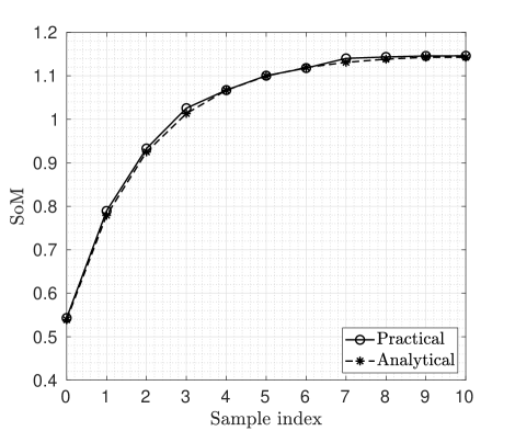
Figure 1: The practical and analytical SoM of the starting samples of an OFDM symbol.

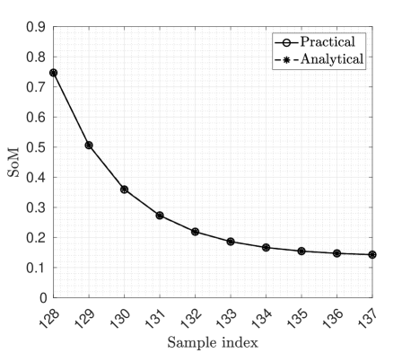
Figure 2: The practical and analytical SoM of the trailing samples of an OFDM symbol.

III-B TO Estimation

In the asymptotic case, $\hat{d}$ is $d\in\mathcal{D}$ that satisfies all the

to estimate TO $d$, we need to iterate over different values of $d\in\mathcal{D}$, and find the one that satisfies all the equations makes the set of equalities in either (III-A) (and (19)) or (22) hold. However, since the number of the received samples $L$ at the receiver is finite, the equalities in Equations (III-A) and (22) turn into semi-equalities meaning that the values would be very close but not equal for an optimal $d$. Thus, we need to compromise here and use the absolute value of differences as follows

$$\min_{d\in\mathcal{D}}\sum_{k=0}^{n_{\rm{s}}-1} \Big{\lvert}\hat{M}^{-}_{d,L}[k]-M_{0}[k+\lvert d\rvert]\Big{\rvert}~{}u[-d]$$ (23)

$$~{}+\Big{\lvert}\hat{M}^{+}_{d,L}[k]-M_{0}[k]\Big{\rvert}u[d-1]+\Big{\lvert}\hat{M}^{\text{noise}}_{d}-\sigma^{2}_{n}\Big{\rvert}u[d-1]$$

where $u[d]$ is discrete unit step function, defined as

$$u[k]=\begin{cases}1,&k\geq 0\\ 0,&k<0.\end{cases}$$ (24)

From Eq. (23), it is clear that the accuracy of the estimator heavily depends on how large the number of the received samples $L$ is. This is a limiting factor in resource-limited devices where a large number of OFDM symbols cannot be loaded into memory. Hence, affecting the accuracy of the estimation. In order to address this issue and achieve higher accuracy, we will improve the estimator in Eq. (23) in the next subsection.

III-C Weighted SoM estimator for SISO-OFDM

In this subsection, we propose and develop the weighted second order moment (WSOM) estimator that offers a higher probability of lock-in. The main idea of WSOM estimator is to give each sample’s moment a weight which describes the confidence on the closeness of the analytical and practical means.

The variance of a random variable approximately shows how close on average is the realization value of a random value to its mean value. In our case, the mean value is the second moments of the samples we derived in Theorem 1, and the variance of those second moments shows how close on average the second moments of the received samples, i.e. the left hand sides in Eq. (III-A) and (22) would be to their mean value, i.e. the right hand sides in Eq. (III-A) and (22). That is, the smaller the variance, the closer the second moments of the received samples, i.e. the left hand sides in Eq. (III-A) and (22), would be to their mean value, i.e. the right hand sides in Eq. (III-A) and (22). Hence, the inverse of the variance of $|y^{(n)}[k]|^{2},k=1,\ldots,n_{\rm s}$ shows our confidence in how close the left and right hand sides of Equations (III-A) and (22) are. Next Theorem provides the variance of the SoM of the received samples

Theorem 2.

The variance of the SoMs of different received OFDM samples are given as follows

$$\begin{split}\sigma^{2}_{|y^{(n)}[k]|^{2}|{\rm{H}}_{0}}=\frac{13}{4}\sigma^{4}_{s}\sum_{l=a_{k}}^{b_{k}}\sigma^{4}_{h_{l}}+\frac{5}{2}\sigma^{4}_{s}\sum_{r=a_{k}}^{r=b_{k}}\sum_{l=a_{k},l\neq r}^{l=b_{k}}\sigma^{2}_{h_{l}}\sigma^{2}_{h_{r}}\\ +2~{}\sigma^{2}_{n}\sigma^{2}_{s}\sum_{l=a_{k}}^{b_{k}}\sigma^{2}_{h_{l}}+\sigma^{4}_{n}-\frac{1}{4}\sigma^{2}_{s}\big{(}\sum_{l=a_{k}}^{b_{k}}\sigma^{2}_{h_{l}}\big{)}^{2}\end{split}$$ (25)

where $n\in\mathbb{Z}_{\geq 0}$,

$$(a_{k},b_{k})=\begin{cases}(0,k)&~{}0\leq k\leq n_{\rm{h}}-2\\ (0,n_{\rm{h}}-1)&~{}n_{\rm{h}}-1\leq k\leq n_{\rm{x}}-1\\ (k-n_{\rm{x}}+1,n_{\rm{h}}-1)&~{}n_{\rm{x}}\leq k\leq n_{\rm{x}}+n_{\rm{h}}-2.\end{cases}$$ (26)

and it is equal to $2\sigma^{2}_{n}$ for $n_{\rm{x}}+n_{\rm{h}}-1\leq k\leq n_{\rm{s}}-1$.

Proof.

See Appendix V. ∎

Figures 3 and 4 show the asymptotic convergence of the variance of the SoMs of the starting and trailing samples for an OFDM symbol with $10^{5}$ Monte Carlo realizations.

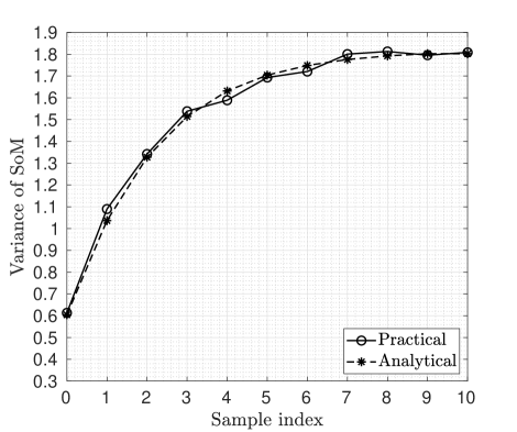
Figure 3: The practical and analytical variance of SoM of the starting samples for an OFDM symbol.

Now, we use the inverse of the variance of the SoMs, given in Theorem 2, as weights in Eq. (23) to improve the accuracy of the estimator. Let us define

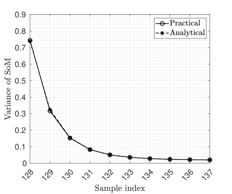
Figure 4: The practical and analytical variance of SoM of the trailing samples for an OFDM symbol.

$$F[k+nn_{\rm{s}}]\triangleq ~{}\sigma^{2}_{|y^{(n)}[k]|^{2}|{\rm{H}}_{0}}$$

$$F^{\text{noise}}\triangleq 2\sigma^{2}_{n},$$ (27)

$$\forall k\in\{0,1,\cdots,n_{\rm{s}}-1\},$$

$$\forall n\in\mathbb{Z}_{\geq 0}.$$

Clearly, each $F[i]$ maps to $M_{0}[i]$ defined in Theorem 1, hence, one can write the weighted version of the estimator in Eq. (23) as

$$\min_{d\in\mathcal{D}}\sum_{k=0}^{n_{\rm{s}}-1} \frac{1}{F[k+\lvert d\rvert]}\Big{\lvert}\hat{M}^{-}_{d,L}[k]-M_{0}[k+\lvert d\rvert]\Big{\rvert}~{}u[-d]$$ (28)

$$~{}+\frac{1}{F[k]}\Big{\lvert}\hat{M}^{+}_{d,L}[k]-M_{0}[k]\Big{\rvert}u[d-1]$$

$$+\frac{1}{F^{\text{noise}}}\Big{\lvert}\hat{M}^{\text{noise}}_{d}-\sigma^{2}_{n}\Big{\rvert}u[d-1]$$

This completes our derivation of the WSOM estimator. Next, we generalize the derived estimators in (23) and (28) to MIMO systems.

III-D Extension to MIMO systems

In this subsection, we assume both the transmitter and the receiver have multiple antennas. For the simplicity of derivations, we keep the total power transmitted through multiple transmit antennas equal to that of single antenna transmitter in SISO systems. We also assume the delay at different receive antennas are all equal to $d$.

In order to extend the proposed estimators to MIMO systems, we need to find the accumulative SoM of the received samples at different receive antennas. Let us assume the transmit antennas at the transmitter are used for spatial multiplexing. That is, different signals (information) are sent through different antennas at the transmitter. This means that the SoM of the received samples at the receiver are simply the sum of the SoMs of the received samples coming from each transmit antenna. Using Equations (3) and (4), we can write

$$\mathbb{E}\big{\{}|{\bf y}^{(n)}_{j}[k]|^{2}|{\rm{H}}_{0}\big{\}} =(\sum^{m_{\rm t}}_{i=1}{\bf H}_{ji}{\bf s}^{(n)}_{i})[k]+{\bf w}^{(n)}_{j}[k]$$ (29)

$$=\sum^{m_{\rm t}}_{i=1}\sum_{l=a_{k}}^{b_{k}}\sigma^{2}_{s_{i}}\sigma^{2}_{h_{l}}+\sigma^{2}_{n}$$

$$=\sum^{m_{\rm t}}_{i=1}\sigma^{2}_{s_{i}}\sum_{l=a_{k}}^{b_{k}}\sigma^{2}_{h_{l}}+\sigma^{2}_{n}$$

$$=\sigma^{2}_{s}\sum_{l=a_{k}}^{b_{k}}\sigma^{2}_{h_{l}}+\sigma^{2}_{n}$$

where the last equality comes from the fact that $\sum^{m_{\rm t}}_{i=1}\sigma^{2}_{s_{i}}=\sigma^{2}_{s}$, and $a_{k}$ and $b_{k}$ are given in (14). Hence, the theoretical SoMs for each received sample at each antenna $j$ remain the same as the one in Theorem 1.

Similar to our discussions for SISO systems, the practical SoMs of the received samples can be derived as

$$B^{-}_{d,L}[k]\triangleq ~{}\frac{1}{m_{\rm{r}}\lfloor(L-k+1)/n_{\rm{s}}\rfloor}\times$$

$$~{}~{}~{}~{}~{}~{}~{}~{}~{}~{}~{}~{}~{}~{}~{}\sum_{j=0}^{m_{\rm{r}}-1}\sum_{r=0}^{\lfloor(L-k+1)/n_{\rm{s}}\rfloor-1}|y^{j}_{\text{rec}}[k+rn_{\rm{s}}]|^{2},$$

$$\forall k\in\{0,1,\cdots,n_{\rm{s}}-1\}.$$

where $y^{j}_{\text{rec}}$ denotes the vector of the received samples at the $j$-th receive antenna. Similarly, for $d>0$, one can write

$$B^{\text{noise}}_{d}=\frac{1}{d}\sum_{j=0}^{m_{\rm{r}}-1}\sum_{r=0}^{d-1}|y^{j}_{\text{rec}}[r]|^{2}.$$ (30)

and

$$B^{+}_{d,L}[k]= \frac{1}{m_{\rm{r}}\lfloor(L-k+1)/n_{\rm{s}}\rfloor}\times$$

$$~{}~{}~{}~{}~{}\sum_{j=0}^{m_{\rm{r}}-1}\sum_{r=0}^{\lfloor(L-k-d+1)/n_{\rm{s}}\rfloor-1}|y^{j}_{\text{rec}}[k+d+rn_{\rm{s}}]|^{2},$$

$$\forall k\in\{0,1,\cdots,n_{\rm{s}}-1\}.$$ (31)

One can then write the TO estimator for the MIMO systems as

$$\min_{d\in\mathcal{D}}\sum_{k=0}^{n_{\rm{s}}-1} \frac{1}{F[k+\lvert d\rvert]}\Big{\lvert}B^{-}_{d,L}[k]-M_{0}[k+\lvert d\rvert]\Big{\rvert}~{}u[-d]$$ (32)

$$~{}+\Bigg{(}\frac{1}{F[k]}\Big{\lvert}B^{+}_{d,L}[k]-M_{0}[k]\Big{\rvert}$$

$$~{}~{}~{}~{}~{}~{}~{}~{}~{}~{}~{}~{}~{}~{}~{}~{}~{}~{}~{}~{}~{}+\frac{1}{F^{\text{noise}}}\Big{\lvert}B^{\text{noise}}_{d}-\sigma^{2}_{n}\Big{\rvert}\Bigg{)}u[d-1]$$

One can replace $F[i]$s and $F^{\text{noise}}$s with ones to obtain the unweighted estimator for MIMO systems. Eq. (32) as the most general from of the proposed TO estimators for MIMO systems is expanded in Eq. (33).

Deriving an upper bound for the complexity of the TO estimator proposed in Eq. (32) is very easy. It should be noted that the weights $F[i]$s and $F^{\text{noise}}$s can be calculated once before any signal reception; hence, the complexity of the SoM estimator in Eq. (32) is equal to $\mathcal{O}(m_{\rm r}L)$ which is significantly lower than the one in [14].

$$\min_{d\in\mathcal{D}}\sum_{k=0}^{n_{\rm{s}}-1} \frac{\Big{\lvert}\frac{1}{m_{\rm{r}}\lfloor(L-k+1)/n_{\rm{s}}\rfloor}\sum_{j=0}^{m_{\rm{r}}-1}\sum_{r=0}^{\lfloor(L-k+1)/n_{\rm{s}}\rfloor-1}|y^{j}_{\text{rec}}[k+rn_{\rm{s}}]|^{2}-\sigma^{2}_{s}\sum_{l=a_{k+\lvert d\rvert}}^{b_{k+\lvert d\rvert}}\sigma^{2}_{h_{l}}-\sigma^{2}_{n}\Big{\rvert}~{}u[-d]}{\frac{13}{4}\sigma^{4}_{s}\sum_{l=a_{k+\lvert d\rvert}}^{b_{k+\lvert d\rvert}}\sigma^{4}_{h_{l}}+\frac{5}{2}\sigma^{4}_{s}\sum_{r=a_{k+\lvert d\rvert}}^{r=b_{k+\lvert d\rvert}}\sum_{l=a_{k+\lvert d\rvert},l\neq r}^{l=b_{k+\lvert d\rvert}}\sigma^{2}_{h_{l}}\sigma^{2}_{h_{r}}+2~{}\sigma^{2}_{n}\sigma^{2}_{s}\sum_{l=a_{k+\lvert d\rvert}}^{b_{k+\lvert d\rvert}}\sigma^{2}_{h_{l}}+\sigma^{4}_{n}-\frac{1}{4}\sigma^{2}_{s}\big{(}\sum_{l=a_{k+\lvert d\rvert}}^{b_{k+\lvert d\rvert}}\sigma^{2}_{h_{l}}\big{)}^{2}}$$ (33)

$$~{}+\frac{\Big{\lvert}\frac{1}{m_{\rm{r}}\lfloor(L-k+1)/n_{\rm{s}}\rfloor}\sum_{j=0}^{m_{\rm{r}}-1}\sum_{r=0}^{\lfloor(L-k-d+1)/n_{\rm{s}}\rfloor-1}|y^{j}_{\text{rec}}[k+d+rn_{\rm{s}}]|^{2}-\sigma^{2}_{s}\sum_{l=a_{k}}^{b_{k}}\sigma^{2}_{h_{l}}-\sigma^{2}_{n}\Big{\rvert}~{}u[d-1]}{\frac{13}{4}\sigma^{4}_{s}\sum_{l=a_{k}}^{b_{k}}\sigma^{4}_{h_{l}}+\frac{5}{2}\sigma^{4}_{s}\sum_{r=a_{k}}^{r=b_{k}}\sum_{l=a_{k},l\neq r}^{l=b_{k}}\sigma^{2}_{h_{l}}\sigma^{2}_{h_{r}}+2~{}\sigma^{2}_{n}\sigma^{2}_{s}\sum_{l=a_{k}}^{b_{k}}\sigma^{2}_{h_{l}}+\sigma^{4}_{n}-\frac{1}{4}\sigma^{2}_{s}\big{(}\sum_{l=a_{k}}^{b_{k}}\sigma^{2}_{h_{l}}\big{)}^{2}}$$

$$~{}~{}~{}~{}~{}~{}~{}~{}~{}~{}~{}~{}~{}~{}~{}~{}~{}~{}~{}~{}~{}+\frac{1}{2\sigma^{2}_{n}}\Big{\lvert}\frac{1}{d}\sum_{j=0}^{m_{\rm{r}}-1}\sum_{r=0}^{d-1}|y^{j}_{\text{rec}}[r]|^{2}-\sigma^{2}_{n}\Big{\rvert}u[d-1]$$

 

IV Simulation results

In this section, we investigate the performance of the proposed SoM and its weighted version through extensive simulation results under various scenarios.

As shown in Appendix LABEL:??????????, one can easily show that

IV-A Simulation Setup

We consider a ZP-OFDM system in a doubly-selective (frequency and time) Rayleigh channel. 128-QAM modulation scheme is used for data transmission. If otherwise not specified, the number of data symbols is $n_{\rm{x}}=128$ and the number of zero-padding samples are $n_{\rm{z}}=12$. The number of received OFDM symbols, i.e. $N$, used for estimation is 10. The transmit power is set to $\sigma_{\rm{x}}^{2}=1$.

The sampling frequency at the receiver is set to $f_{\rm sa}=10^{9}$. A multipath fading channel with maximum delay spread of $\tau_{\rm{max}}=10$ns, equivalent to $n_{\rm{h}}=10$ taps, is assumed. An exponential decaying function, i.e., $\sigma^{2}_{h_{l}}=\alpha\exp(-\beta l)$, $l=0,1,\dots,n_{\rm{h}}-1$, where $p_{\rm{h}}=\sum_{l=0}^{n_{\rm{h}}-1}\sigma^{2}_{h_{l}}=1$, $\alpha=1/2.5244$, and $\beta=0.5$, is considered for the delay profile of the fading channel. The maximum Doppler spread of the channel is assumed to be $f_{\rm{D}}=150$ Hz.

An additive white Gaussian noise (AWGN) is considered and modeled as a zero-mean complex Gaussian random variable with variance $\sigma^{2}_{\rm{w}}$ derived based on the value of $E_{\rm{b}}/N_{0}$. The TO affecting the system is modeled as an integer random variable uniformly distributed in the range $d\in[-30,\ 30]$. The number of Monte Carlo realization is set to $10^{4}$ for all simulation setups. A strict performance measure, i.e. lock-in probability, is used to measure the effectiveness of the proposed estimators. Lock-in probability here refers the probability that the estimated TO is equal to the actual TO. Hence, any non-zero estimation error is considered a missed estimation.

IV-B Simulation Results

We compare the performance of the proposed SoM estimator and its improved weighted version versus the current state-of-the-art estimator proposed by other authors in [17], i.e. transition metric transition metric (TM). The lock-in probability of the proposed estimators versus TM for different values of $E_{\rm{b}}/N_{0}$ are shown in Fig. 5. As can be seen, there is a performance gap between the proposed estimators and TM while weighted SoM having the highest probability of lock-in amongst all. This is due to the fact that weighted SoM takes advantage of the statistical information of the channel. The performance of the weighted SoM improves as $E_{\rm{b}}/N_{0}$ increases because our confidence, modeled as the weights, in the derived theoretical second-order moment, and its closeness to the actual second-order moment of each received sample increases. However, the importance of the proposed estimators manifest itself in lower SNRs, i.e. 0 to -10 dB, where the lock-in probability is still at 40% compared to TM with negligible lock-in probability. Also, note that unlike [14], the proposed estimators can perform for values under 5dB.

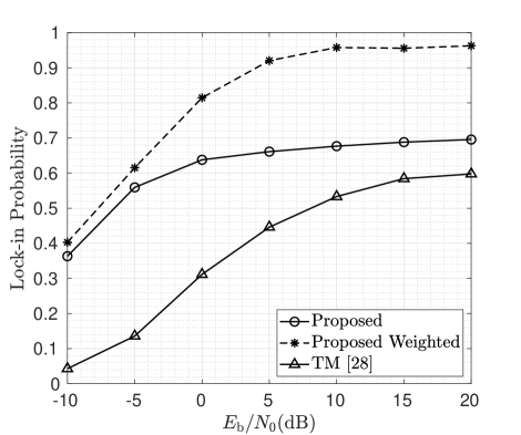
Figure 5: Lock-in probability versus $E_{\rm{b}}/N_{0}$.

The effect of the maximum Doppler spread in Hz (speed of mobility) on the performance of the proposed estimators are shown in Fig. 6. As seen, the proposed estimators, unlike [14], are relatively independent of the maximum Doppler shift (movement speed). This is mainly due to the fact that unlike [14] where the joint PDF of the received samples is approximated via independency assumption between channel taps, the proposed estimators do not heavily rely on the independency of different channel taps. This makes the proposed estimators an appealing solution for very low to very high speed applications.

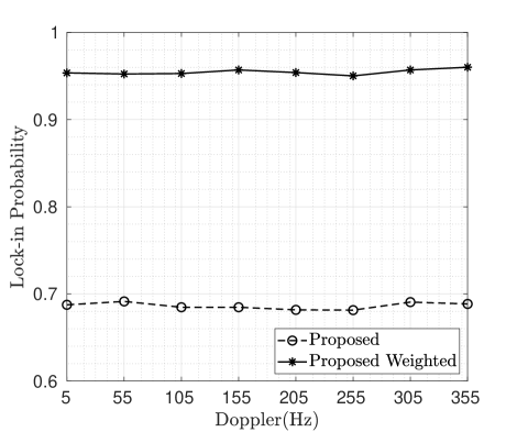
Figure 6: Lock-in probability versus maximum Doppler spread of the fading channel at $15$ dB $E_{\rm{b}}/N_{0}$.

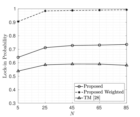
Figure 7: Lock-in probability versus the number of observation vectors $N$ at $15$ dB $E_{\rm{b}}/N_{0}$.

Figure 7 illustrates the effect of the number of the observation OFDM symbols used for estimation, on the performance of the proposed estimators. As expected, the probability of lock-in increases as the number of observation samples used for estimation increases. The improvements, however, decreases as the number of observation symbols increases. This is because the new information that each new sample adds to the second-order moment and its variance decreases as the number of samples grows.

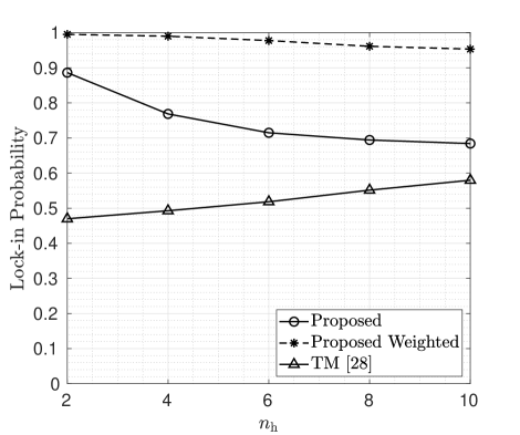
Figure 8: Lock-in probability versus the number of channel taps $n_{\rm{h}}$ at $15$ dB $E_{\rm{b}}/N_{0}$.

The performance of the proposed estimators and TM for different values of the number of channel taps $n_{\rm{h}}$, is shown in Fig. 8. The lock-in probability of the proposed estimators decreases as the number of channel taps increases. This is because the deviation of the theoretical SoM in (13) from the actual value increases as the number of channel taps increases. As expected, this decrease in lock-in probability is heavier in unweighted version where the only information is used for estimation is (13).

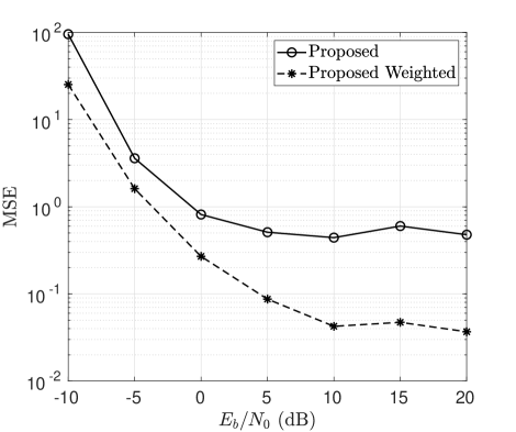
Figure 9: MSE versus $E_{\rm{b}}/N_{0}$. .

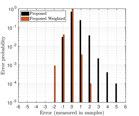
Figure 10: PMF of the synchronization error at 15 dB $E_{\rm{b}}/N_{0}$.

The empirical probability mass function (PMF) of the synchronization error for the proposed estimators are shown in Fig. 10. As seen, the PMF of the error for weighted SoM is relatively unbiased, while the unweighted SoM is biased towards positive values. Notice, however, that the estimation error for weighted SoM is limited to a range of maximum two neighbouring samples from each side which results in low mean-squared error (MSE) as shown in Fig. 9. Fig. 9 also shows an average estimation error of less than two for very low SNR, i.e. -5 dB, for the weighted SoM. Hence, simple and modified versions of the weighted SoM where neighbouring samples of the estimated TO are also checked can be devised to achieve 100% lock-in probability.

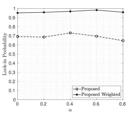
Figure 11: Sensitivity of the proposed synchronization algorithms to PDP estimation error for $N=10$ at 15 dB $E_{\rm{b}}/N_{0}$.

Fig. 11 shows the effect of power delay profile (PDP) estimation error on the lock-in probability. The estimated PDP used for estimation is randomly uniform set to be either $\sigma^{2}_{{\rm{h}}_{k}}-\alpha\sigma^{2}_{{\rm{h}}_{k}}$ or $\sigma^{2}_{{\rm{h}}_{k}}+\alpha\sigma^{2}_{{\rm{h}}_{k}}$ where $\sigma^{2}_{{\rm{h}}_{k}}$, $k=0,1,\dots,n_{\rm{h}}-1$, is the true PDP, and $\alpha\in[0,0.8]$ denotes the PDP estimation error. As seen, the proposed estimators are relatively robust even for PDP estimation errors larger than $50\%$. Note, however, that the lock-in probability of the weighted SoM remains above $90\%$ even when the the PDP estimation error is about $80\%$.

V Conclusion

In this paper, we proposed two low-complexity NDA TO estimators based on SoM for MIMO ZP-OFDM systems in doubly selective channels. Unlike other estimators in the literature, the proposed estimators enjoy very low complexity, are feasible for very low SNRs, and have very high lock-in probability. Simulation results verify our analysis and demonstrate very high probability of lock-in for the proposed estimators making them suitable for implementation in low-power low complexity devices, i.e. IoT devices and underwater sensors, unlike the other NDA TO estimators for ZP-OFDM systems.

Proof.

For notation simplicity and without loss of generality, we omit the $\ldots|{\rm{H}}_{0}$ from equations. For mathematical simplicity, we consider $d=0$ because non-zero delays are easily derived, mostly via a shift, from zero delay case. We have $\sigma^{2}_{|y_{n}[k]|^{2}}=\mathbb{E}\{|y_{n}[k]|^{4}\}-\mathbb{E}\{|y_{n}[k]|^{2}\}^{2}$. The second term, $\mathbb{E}\{|y_{n}[k]|^{2}\}$ has been derived before, and so we need to only focus on $\mathbb{E}\{|y_{n}[k]|^{4}\}$. Note that

$$\begin{split}\mathbb{E}\{|y_{n}[k]|^{4}\}&=\mathbb{E}\bigg{\{}\big{(}v^{(n)}[k]+w^{(n)}[k]\big{)}\big{(}v^{(n)}[k]^{*}+w^{(n)}[k]^{*}\big{)}\\ &~{}~{}~{}~{}~{}~{}~{}~{}\big{(}v^{(n)}[k]+w^{(n)}[k]\big{)}\big{(}v^{(n)}[k]^{*}+w^{(n)}[k]^{*}\big{)}\bigg{\}}\\ &=\mathbb{E}\bigg{\{}\bigg{(}|v^{(n)}[k]|^{2}+v^{(n)}[k]w^{(n)}[k]^{*}+\\ &~{}~{}~{}~{}~{}~{}~{}~{}~{}~{}~{}~{}~{}~{}~{}~{}~{}~{}~{}v^{(n)}[k]^{*}w^{(n)}[k]+|w^{(n)}[k]|^{2}\bigg{)}^{2}\bigg{\}}\\ &\stackrel{{\scriptstyle a}}{{=}}\mathbb{E}\bigg{\{}|v^{(n)}[k]|^{4}+4|v^{(n)}[k]|^{2}|w^{(n)}[k]|^{2}+\\ &~{}~{}~{}~{}~{}~{}~{}~{}~{}~{}~{}|w^{(n)}[k]|^{4}+v^{(n)}[k]^{2}{w^{(n)}[k]^{*}}^{2}+\\ &~{}~{}~{}~{}~{}~{}~{}~{}~{}~{}~{}~{}~{}~{}~{}~{}~{}~{}~{}{v^{(n)}[k]^{*}}^{2}w^{(n)}[k]^{2}\bigg{\}}\\ &\stackrel{{\scriptstyle b}}{{=}}\mathbb{E}\Big{\{}|v^{(n)}[k]|^{4}\Big{\}}+4\mathbb{E}\Big{\{}|v^{(n)}[k]|^{2}\Big{\}}\mathbb{E}\Big{\{}|w^{(n)}[k]|^{2}\Big{\}}\\ &~{}~{}~{}~{}~{}~{}~{}~{}~{}~{}~{}+\mathbb{E}\Big{\{}|w^{(n)}[k]|^{4}\Big{\}}\end{split}$$ (34)

where (a) comes from the fact that $v^{(n)}[k]$ and $w^{(n)}[k]$ are independent complex random variables, and $\mathbb{E}\{v^{(n)}[k]\}=\mathbb{E}\{w^{(n)}[k]\}=0$ and (b) is easy to show that $\mathbb{E}\{v^{(n)}[k]^{2}{w^{(n)}[k]^{*}}^{2}+{v^{(n)}[k]^{*}}^{2}w^{(n)}[k]^{2}\}=0$. We have derived $\mathbb{E}\{|v^{(n)}[k]|^{2}\}$ in previous sections. Also, since $w^{(n)}[k]$ is a complex random variable, we have $\mathbb{E}\{|w^{(n)}[k]|^{2}\}=\sigma^{2}_{w}$ and $\mathbb{E}\{|w^{(n)}[k]|^{4}\}=2\sigma^{4}_{w}$. Hence, the problem further boils down to deriving $\mathbb{E}\{|v^{(n)}[k]|^{4}\}$. After some extensive mathematical manipulation, one can show that

$$\begin{split}&\mathbb{E}\{|v^{(n)}[k]|^{4}\}\\ &=\mathbb{E}\Bigg{\{}\Bigg{(}\bigg{(}\sum^{b}_{u=a}h_{\rm{I}}[k,u]s^{(n)}_{{\rm{I}}}[k-u]-h_{\rm{Q}}[k,u]s^{(n)}_{{\rm{Q}}}[k-u]\bigg{)}^{2}\\ &~{}+\bigg{(}\sum^{b}_{u=a}h_{\rm{I}}[k,u]s^{(n)}_{{\rm{Q}}}[k-u]+h_{\rm{Q}}[k,u]s^{(n)}_{{\rm{I}}}[k-u]\bigg{)}^{2}\Bigg{)}^{2}\Bigg{\}}\\ &=\mathbb{E}\Bigg{\{}\bigg{(}\sum^{b}_{u=a}h_{\rm{I}}[k,u]s^{(n)}_{{\rm{I}}}[k-u]-h_{\rm{Q}}[k,u]s^{(n)}_{{\rm{Q}}}[k-u]\bigg{)}^{4}\Bigg{\}}\\ &+\mathbb{E}\Bigg{\{}\bigg{(}\sum^{b}_{u=a}h_{\rm{I}}[k,u]s^{(n)}_{{\rm{Q}}}[k-u]+h_{\rm{Q}}[k,u]s^{(n)}_{{\rm{I}}}[k-u]\bigg{)}^{4}\Bigg{\}}\\ &+2~{}\mathbb{E}\Bigg{\{}\bigg{(}\sum^{b}_{u=a}h_{\rm{I}}[k,u]s^{(n)}_{{\rm{I}}}[k-u]-h_{\rm{Q}}[k,u]s^{(n)}_{{\rm{Q}}}[k-u]\bigg{)}^{2}\\ &~{}~{}~{}~{}~{}~{}~{}~{}~{}~{}~{}\bigg{(}\sum^{b}_{u=a}h_{\rm{I}}[k,u]s^{(n)}_{{\rm{Q}}}[k-u]+h_{\rm{Q}}[k,u]s^{(n)}_{{\rm{I}}}[k-u]\bigg{)}^{2}\Bigg{\}}\\ &\stackrel{{\scriptstyle(i)}}{{=}}2~{}\mathbb{E}\Bigg{\{}\bigg{(}\sum^{b}_{u=a}h_{\rm{I}}[k,u]s^{(n)}_{{\rm{I}}}[k-u]-h_{\rm{Q}}[k,u]s^{(n)}_{{\rm{Q}}}[k-u]\bigg{)}^{4}\Bigg{\}}\\ &~{}~{}~{}+2~{}\mathbb{E}\Bigg{\{}\bigg{(}\sum^{b}_{u=a}h_{\rm{I}}[k,u]s^{(n)}_{{\rm{I}}}[k-u]-h_{\rm{Q}}[k,u]s^{(n)}_{{\rm{Q}}}[k-u]\bigg{)}^{2}\\ &~{}~{}~{}~{}~{}~{}~{}~{}~{}~{}~{}~{}\bigg{(}\sum^{b}_{u=a}h_{\rm{I}}[k,u]s^{(n)}_{{\rm{Q}}}[k-u]+h_{\rm{Q}}[k,u]s^{(n)}_{{\rm{I}}}[k-u]\bigg{)}^{2}\Bigg{\}}\end{split}$$ (35)

where (i) comes from the fact that $-h_{\rm{Q}}[k,u]$ and $h_{\rm{Q}}[k,u]$ have the same distribution, i.e. both are Gaussian random variables with zero mean and variance of $\displaystyle\frac{\sigma^{2}_{h_{u}}}{2}$. After some extensive mathematical manipulations and using the facts that (i) in-phase and quadrature components are independent (ii) channel taps with different delays are independent, one can show that

$$\begin{split}&\mathbb{E}\Bigg{\{}\bigg{(}\sum^{b}_{u=a}h_{\rm{I}}[k,u]s^{(n)}_{{\rm{I}}}[k-u]-h_{\rm{Q}}[k,u]s^{(n)}_{{\rm{Q}}}[k-u]\bigg{)}^{4}\Bigg{\}}\\ &=2~{}\mathbb{E}\big{\{}s^{(n)}_{{\rm{I}}}[k-u]^{4}\big{\}}\sum^{b}_{u=a}\mathbb{E}\big{\{}h_{\rm{I}}[k,u]^{4}\big{\}}~{}~{}+\\ &~{}~{}~{}~{}12~{}\mathbb{E}\big{\{}s^{(n)}_{{\rm{I}}}[k-u]^{2}\big{\}}^{2}\sum_{r=a}^{r=b}\sum_{l=a,l\neq r}^{l=b}\mathbb{E}\big{\{}h_{\rm{I}}[k,l]^{2}\big{\}}\mathbb{E}\big{\{}h_{\rm{I}}[k,r]^{2}\big{\}}\\ &~{}~{}~{}~{}+6~{}\mathbb{E}\big{\{}s^{(n)}_{{\rm{I}}}[k-u]^{2}\big{\}}^{2}\bigg{(}\mathbb{E}\big{\{}h_{\rm{I}}[k,u]^{2}\big{\}}\bigg{)}^{2}\\ &=\frac{9}{8}\sigma^{4}_{s}\sum^{b}_{u=a}\sigma^{4}_{h_{u}}+\frac{3}{4}~{}\sigma^{4}_{s}\sum_{r=a}^{r=b}\sum_{l=a,l\neq r}^{l=b}\sigma^{2}_{h_{l}}\sigma^{2}_{h_{r}}+\frac{3}{8}~{}\sigma^{4}_{s}\bigg{(}\sum_{l=a}^{b}\sigma^{2}_{h_{l}}\bigg{)}^{2}\end{split}$$ (36)

Similarly, one can verify that

$$\begin{split}&\mathbb{E}\Bigg{\{}\bigg{(}\sum^{b}_{u=a}h_{\rm{I}}[k,u]s^{(n)}_{{\rm{I}}}[k-u]-h_{\rm{Q}}[k,u]s^{(n)}_{{\rm{Q}}}[k-u]\bigg{)}^{2}\\ &\bigg{(}\sum^{b}_{u=a}h_{\rm{I}}[k,u]s^{(n)}_{{\rm{Q}}}[k-u]+h_{\rm{Q}}[k,u]s^{(n)}_{{\rm{I}}}[k-u]\bigg{)}^{2}\Bigg{\}}\\ &=4~{}\mathbb{E}\big{\{}s^{(n)}_{{\rm{I}}}[k-u]^{2}\big{\}}^{2}\sum_{l=a}^{l=b}\mathbb{E}\big{\{}h_{\rm{I}}[k,l]^{4}\big{\}}~{}~{}+\\ &16~{}\mathbb{E}\big{\{}s^{(n)}_{{\rm{I}}}[k-u]^{2}\big{\}}^{2}\sum_{r=a}^{r=b}\sum_{l=a,l\neq r}^{l=b}\mathbb{E}\big{\{}h_{\rm{I}}[k,l]^{2}\big{\}}\mathbb{E}\big{\{}h_{\rm{I}}[k,r]^{2}\big{\}}\\ &+\bigg{(}4~{}\mathbb{E}\big{\{}s^{(n)}_{{\rm{I}}}[k-u]^{4}\big{\}}-8~{}\mathbb{E}\big{\{}s^{(n)}_{{\rm{I}}}[k-u]^{2}\big{\}}^{2}\bigg{)}\\ &~{}~{}~{}~{}~{}~{}~{}~{}~{}~{}\times\sum_{l=a}^{l=b}\big{(}\mathbb{E}\big{\{}h_{\rm{I}}[k,l]^{2}\big{\}}\big{)}^{2}\\ &=\sigma^{4}_{s}\bigg{(}\sum^{b}_{u=a}\sigma^{4}_{h_{u}}+\sum_{r=a}^{r=b}\sum_{l=a,l\neq r}^{l=b}\sigma^{2}_{h_{l}}\sigma^{2}_{h_{r}}\bigg{)}\end{split}$$ (37)

Substituting Equations (36) and (37) in Equation (35) and then in Equation (34) yields Equation (25). One can easily show that the variance of the SoM of a complex Gaussian random variable $w$ with zero mean and variance $\sigma^{2}_{n}$ is

$$\sigma^{2}_{|w|^{2}}=2\sigma^{2}_{n}.$$ (38)

This completes the proof. ∎

References

- [1] B. Lu and X. Wang, “Space-time code design in ofdm systems,” in Proc. IEEE GLOBECOM, vol. 2, San Francisco, CA, USA, 2000, pp. 1000–1004.
- [2] L. Dai, Z. Wang, J. Wang, and Z. Yang, “Positioning with OFDM signals for the next-generation GNSS,” IEEE Trans. Consum. Electron., vol. 56, no. 2, pp. 374–379, May 2010.
- [3] C. D. Murphy, “Low-complexity FFT structures for OFDM transceivers,” IEEE Trans. Commun., vol. 50, no. 12, pp. 1878–1881, Dec. 2002.
- [4] S. Huang and S. Chen, “A green FFT processor with 2.5-GS/s for IEEE 802.15.3c (WPANs),” in Proc. ICGCS, Shanghai, China, Jun. 2010, pp. 9–13.
- [5] V. P. G. Jimenez, M.-G. Garcia, F. G. Serrano, and A. G. Armada, “Design and implementation of synchronization and AGC for OFDM-based WLAN receivers,” IEEE Trans. Consum. Electron., vol. 50, no. 4, pp. 1016–1025, Nov. 2004.
- [6] M. Kim and S. Chang, “A consumer transceiver for long-range IoT communications in emergency environments,” IEEE Trans. Consum. Electron., vol. 62, no. 3, pp. 226–234, Aug. 2016.
- [7] S.-G. Kim, H.-S. Kim, and S.-H. Park, “Apparatus and method for receiving digital multimedia broadcasting in a wireless terminal,” Oct. 21 2008, US Patent 7,440,516.
- [8] D. C. Alves, G. S. da Silva, E. R. de Lima, C. G. Chaves, D. Urdaneta, T. Perez, and M. Garcia, “Architecture design and implementation of key components of an OFDM transceiver for IEEE 802.15.4g,” in Proc. IEEE ISCAS, Montreal, QC, Canada, May 2016, pp. 550–553.
- [9] X. Wang, P. Ho, and Y. Wu, “Robust channel estimation and ISI cancellation for OFDM systems with suppressed features,” IEEE J. Sel. Areas Commun., vol. 23, no. 5, pp. 963–972, May 2005.
- [10] S. Roy and C. Li, “A subspace blind channel estimation method for OFDM systems without cyclic prefix,” IEEE Trans. Wireless Commun., vol. 1, no. 4, pp. 572–579, Oct. 2002.
- [11] B. Muquet, M. de Courville, G. B. Giannakis, Z. Wang, and P. Duhamel, “Reduced complexity equalizers for zero-padded OFDM transmissions,” in Proc. IEEE ICASSP, Istanbul, Turkey, 2000, pp. 2973–2976.
- [12] F. Tufvesson, O. Edfors, and M. Faulkner, “Time and frequency synchronization for OFDM using PN-sequence preambles,” in Gateway to 21st Century Communications Village. in Proc. IEEE VTC, vol. 4, The Netherlands, Fall 1999, pp. 2203–2207.
- [13] B. Muquet, Z. Wang, G. B. Giannakis, M. de Courville, and P. Duhamel, “Cyclic prefixing or zero padding for wireless multicarrier transmissions?” IEEE Trans. Commun., vol. 50, no. 12, pp. 2136–2148, Dec 2002.
- [14] M. A. K.P. Roshandeh, M. MohammadKarimi, “Maximum likelihood time synchronization forzero-padded ofdm,” submitted to IEEE Trans. Signal Process.
- [15] A. A. Nasir, S. Durrani, H. Mehrpouyan, S. D. Blostein, and R. A. Kennedy, “Timing and carrier synchronization in wireless communication systems: a survey and classification of research in the last 5 years,” EURASIP Journal on Wireless Communications and Networking, no. 1, p. 180, Dec. 2016.
- [16] H. Bolcskei, “Blind estimation of symbol timing and carrier frequency offset in wireless OFDM systems,” IEEE Trans. Commun., vol. 49, no. 6, pp. 988–999, Jun. 2001.
- [17] V. Le Nir, T. van Waterschoot, J. Duplicy, and M. Moonen, “Blind coarse timing offset estimation for CP-OFDM and ZP-OFDM transmission over frequency selective channels,” EURASIP Journal on Wireless Communications and Networking, vol. 2009, no. 1, p. 262813, Jan. 2010. [Online]. Available: https://doi.org/10.1155/2009/262813
- [18] S. Kay, “Fundamentals of statistical signal processing: estimation theory,” Technometrics, vol. 37, no. 4, pp. 465–466, 1993.
- [19] L. Wang, G. Liu, J. Xue, and K.-K. Wong, “Channel prediction using ordinary differential equations for mimo systems,” IEEE Transactions on Vehicular Technology, 2022.
- [20] S. Wen, G. Liu, F. Xu, L. Zhang, C. Liu, and M. A. Imran, “Ergodic capacity of mimo faster-than-nyquist transmission over triply-selective rayleigh fading channels,” IEEE Transactions on Communications, vol. 70, no. 8, pp. 5046–5058, 2022.
- [21] S. G. Kwak and J. H. Kim, “Central limit theorem: the cornerstone of modern statistics,” Korean journal of anesthesiology, vol. 70, no. 2, pp. 144–156, 2017.
- [22] M. Morelli, C.-C. J. Kuo, and M.-O. Pun, “Synchronization techniques for orthogonal frequency division multiple access (OFDMA): A tutorial review,” Proc. IEEE, vol. 95, no. 7, pp. 1394–1427, Jul. 2007.