Hotter than Expected: HST/WFC3 Phase-resolved Spectroscopy of
a Rare Irradiated Brown Dwarf with Strong Internal Heat Flux

Abstract

With infrared flux contrasts larger than typically seen in hot Jupiter, tidally-locked white dwarf-brown dwarf binaries offer a superior opportunity to investigate atmospheric processes in irradiated atmospheres. NLTT5306 is such a system, with a $M_{\rm{BD}}$=52$\pm$3 M_Jup brown dwarf orbiting a $T_{\rm{eff}}$=7756$\pm$35 K white dwarf with an ultra-short period of $\sim$102 min. We present HST/WFC3 spectroscopic phase curves of NLTT5306, consisting of 47 spectra from 1.1 to 1.7 $\mu$m with an average S/N$\sim$65 per wavelength. We extracted the phase-resolved spectra of the brown dwarf NLTT5306B, finding a small $<$100 K day/night temperature difference ($\sim$5% of the average day-side temperature). Our best-fit model phase curves revealed a complex wavelength-dependence on amplitudes and relative phase offsets, suggesting longitudinal-vertical atmospheric structure. The night-side spectrum was well-fit by a cloudy, non-irradiated atmospheric model while the day-side was best-matched by a cloudy, weakly irradiated model. Additionally, we created a simple radiative energy redistribution model of the atmosphere and found evidence for efficient day-to-night heat redistribution and a moderately high Bond albedo. We also discovered an internal heat flux much higher than expected given the published system age, leading to an age reassessment that resulted in NLTT5306B most likely being much younger. We find that NLTT5306B is the only known significantly irradiated brown dwarf where the global temperature structure is not dominated by external irradiation, but rather its own internal heat. Our study provides an essential insight into the drivers of global circulation and day-to-night heat transport as a function of irradiation, rotation rate, and internal heat.

1 Introduction

Spectroscopic phase curve observations of hot Jupiters (e.g., Knutson et al., 2012; Cowan et al., 2012; Stevenson et al., 2014; Arcangeli et al., 2019; Mikal-Evans et al., 2023) have revealed several hundred Kelvin temperature contrasts between their day and night hemispheres. These temperature contrasts drive a wealth of three-dimensional atmospheric dynamics, such as waves, jets, and turbulence, which have an impact on the three-dimensional atmospheric structure and temperature distribution (see Showman et al., 2020, for a review).

Day-to-night heat transport on hot Jupiters is generally dominated by equatorial jets (Showman & Guillot, 2002). A number of recent studies have been dedicated to understanding how this atmospheric heat transport is affected by various parameters including rotation rate, irradiation strength, and atmospheric composition (Tan & Showman, 2020; Parmentier et al., 2021; Gao & Powell, 2021; Komacek et al., 2022; Lian et al., 2022). Tackling these questions requires high S/N observations capable of measuring heat transport and a sample of objects that continuously span the parameters mentioned above. High S/N observations can be challenging to obtain for hot Jupiters due to the low relative brightness of their host stars. However, there exists another class of objects that experiences levels of irradiation similar to hot Jupiters – white dwarf-brown dwarf (WD+BD) binaries with ultra-short orbital periods (Casewell et al., 2012; Beuermann et al., 2013; Parsons et al., 2017; Casewell et al., 2020b, a). The WD hosts in these binaries not only emit at shorter wavelengths than their main sequence counterparts in hot Jupiter systems, but are also much smaller in size. So, while hot Jupiters suffer from small infrared flux contrasts with their host stars, irradiated brown dwarfs typically exhibit infrared flux contrasts that are at least two orders of magnitude better. This makes WD+BD binaries perfect proxies to hot Jupiters.

WD+BD pairs with ultra-short periods are thought to be the result of common envelope stellar evolution, leaving behind tight binaries that will eventually become cataclysmic variables (Politano, 2004). The extremely short periods of these systems ($\sim$1$-$2 hours) allows observations to capture more orbits in a shorter amount of time, leading to more robust analyses and results. In atmospheric terms, irradiated brown dwarfs act as a bridge between non-irradiated brown dwarfs and irradiated hot Jupiters. For most of the ultra-short period WD+BD systems that have been studied so far, day-side emission is largely dominated by irradiation over internal heat, e.g., WD 0137B (Maxted et al., 2006), SDSS J1205-0242B (Parsons et al., 2017), and EPIC 2122B (Casewell et al., 2018). Thus, observationally testing the interplay between interior heat flux and irradiation along with the impact it has on atmospheric dynamics and thermal structures has not yet been possible.

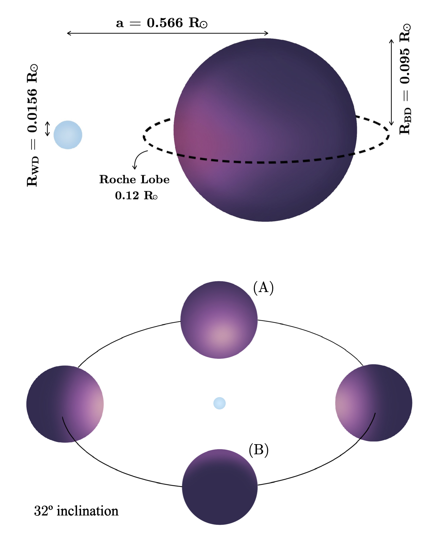
Figure 1: Schematic of NLTT5306. Top: Near edge-on view of NLTT5306, showing relative sizes for the white dwarf, brown dwarf, and brown dwarf Roche Lobe radius. Separation between the white dwarf and brown dwarf are not to scale. Colors correspond to calculated temperatures from spectral fitting. Bottom: NLTT5306 viewed from a hypothesized 32^∘ inclination. To an observer, the day-side of the brown dwarf would be seen when the brown dwarf is in the position labeled (A). Conversely, night would be when the brown dwarf is at the position labeled (B).

Table 1: Properties of the NLTT5306 binary system

Parameter	Units	Value	Reference
$a$	Orbital Separation [R⊙]	0.566$\pm$0.005	Steele et al. (2013)
$i$	Orbital Inclination [deg]	78.0${}^{+1.1}_{-7.6}$	This work
$D$	Distance [pc]	76.96${}^{+0.55}_{-0.53}$	Casewell et al. (2020a)
$P$	Orbital Period [mins]	101.88$\pm$0.02	Steele et al. (2013)
$T_{\rm{eff,WD}}$	Effective Temperature [K]	7756$\pm$35	Steele et al. (2013)
$T_{\rm{eff,BD}}$ (Day)	Effective Temperature [K]	$\sim$1640	This work
$T_{\rm{eff,BD}}$ (Night)	Effective Temperature [K]	$\sim$1500	This work
Spectral Type (BD)		L5	Casewell et al. (2020a)
log $g$ (WD)	Surface Gravity [cm s-2]	7.68$\pm$0.08	Steele et al. (2013)
$M_{\rm{WD}}$	Mass [M⊙]	0.44$\pm$0.04	Steele et al. (2013)
$M_{\rm{BD}}$	Mass [M⊙]	0.05$\pm$0.003	Steele et al. (2013)
Cooling Age (WD)	[Myr]	710$\pm$50	Steele et al. (2013)
$R_{\rm{WD}}$	Radius [R⊙]	0.0156$\pm$0.0016	Steele et al. (2013)
$R_{\rm{BD}}$	Radius [R⊙]	0.095$\pm$0.004	Steele et al. (2013)
$R_{\rm{RL,BD}}$	Roche Lobe Radius [R⊙]	0.12$\pm$0.02	Longstaff et al. (2019)

Atmospheric properties of highly irradiated brown dwarfs have been investigated through 3D circulation models and 1D radiative-convective models (Tan & Showman, 2020; Lothringer & Casewell, 2020; Lee et al., 2020). Tan & Showman (2020) and Lee et al. (2020) both found that the fast rotation rates on irradiated brown dwarfs significantly shrink the width of the predicted equatorial jet and suppress the day-to-night heat transfer. They also found that the day-side hot spot is not subject to eastward-shifting, unlike in hot Jupiter atmospheres (Knutson et al., 2007; Showman & Polvani, 2011; Heng & Showman, 2015; Wong et al., 2016). Lothringer & Casewell (2020) created self-consistent model spectra of brown dwarf atmospheres, incorporating the effect of strong ultraviolet irradiation. They found that in brown dwarf atmospheres that are irradiation-dominated, molecules are efficiently dissociated by the intense irradiation, resulting in atmospheres that resemble ultra-hot Jupiters (Arcangeli et al., 2018; Lothringer et al., 2018; Parmentier et al., 2018; Kitzmann et al., 2018), i.e., no molecular absorption on the day-side. So far, theoretical studies of irradiated brown dwarfs have only considered scenarios in which the brown dwarf receives strong external irradiation. Additionally, all significantly irradiated atmospheres studied to date via high-precision time-series spectroscopy have been irradiation-dominated: WASP-43b (Stevenson et al., 2014); WASP-18b (Arcangeli et al., 2019); WASP-12b (Arcangeli et al., 2021); SDSS1411-B (Lew et al., 2022); WD 0137B and EPIC 2122B (Zhou et al., 2022); and WASP-103b (Kreidberg et al., 2018).

To further our understanding of irradiated substellar atmospheres and their dependencies on rotation rate, internal heat flux, and external irradiation strength, we present Hubble Space Telescope (HST) Wide Field Camera 3 (WFC3) observations of the WD+BD binary system LSPM-J0135+1445 (hereafter NLTT5306). These observations, and those described in Lew et al. (2022) and Zhou et al. (2022), are part of the HST program GO-15947 (PI: Apai). NLTT5306 is a detached binary, estimated to be filling $\approx$80% of its Roche Lobe radius (Figure 1). NLTT5306 also occupies a unique parameter space when compared to the other WD+BD binaries that have already been studied in that its irradiation level is at least an order of magnitude lower, yet its internal heat flux is still quite strong (Showman, 2016).

This paper is organized as follows: In Section 2 we introduce WD+BD system NLTT5306 and relevant findings from previous studies. We describe the details of our observations in Sections 3 and data reduction procedures in 4. In Section 5, we present the broadband light curve along with synthetic phase curves and evidence of relative phase offsets; in Section 6, we extract the phase-resolved spectra of NLTT5306B and derive brightness temperatures from the day- and night-sides. We compare the day and night spectra to field brown dwarfs in Section 7. In Sections 8 and 9, we introduce atmospheric models of non-irradiated and irradiated brown dwarfs, respectively, and compare them to the day-and night-sides of NLTT5306B. In Section 10, we describe a cloud-free general circulation model and examine inconsistencies with observations. We discuss interpretations of our results in Section 11 and summarize our findings in Section 12.

Table 2: Log of HST WFC3 Observations for NLTT5306

Orbit	Observation	Filter	Exp. Time	Exp. Start
	Type	ID	[s]	[BJDTDB]
Visit 1
1	Imaging	F132N	$2\times 29.6=59.2$	2459096.4241
1	Spectroscopic	G141	$8\times 313.1=2504.8$	2459096.4254
2	Imaging	F132N	$2\times 29.6=59.2$	2459096.4903
2	Spectroscopic	G141	$8\times 313.1=2504.8$	2459096.4917
3	Imaging	F132N	$2\times 29.6=59.2$	2459096.5566
3	Spectroscopic	G141	$8\times 313.1=2504.8$	2459096.5579
Inter-visit gap: 797.4 min
Visit 2
4	Imaging	F132N	$2\times 29.6=59.2$	2459097.1522
4	Spectroscopic	G141	$8\times 313.1=2504.8$	2459097.1536
5	Imaging	F132N	$2\times 29.6=59.2$	2459097.2185
5	Spectroscopic	G141	$8\times 313.1=2504.8$	2459097.2199
6	Imaging	F132N	$2\times 29.6=59.2$	2459097.2848
6	Spectroscopic	G141	$8\times 313.1=2504.8$	2459097.2861

Note. — BJD_TDB here was calculated by converting from UT start date and time of observations (DATE-OBS and TIME-OBS in MJD in the flt fits headers) using an online applet developed by Jason Eastman (Eastman et al., 2010).

2 White Dwarf Brown Dwarf
Binary System NLTT5306

NLTT5306 was first suggested to be a binary by Girven et al. (2011) and Steele et al. (2011) who noted the WD exhibited a near-infrared (NIR) excess, which led to the discovery of the brown dwarf companion. Key physical properties of the system are reported in Table 1.

Steele et al. (2013) determined $T_{\rm{eff}}$ = 7756$\pm$35 K and log($g$) = 7.68$\pm$0.08 for the WD, making it the coolest known WD host in a post-common envelope binary (Figure 5 in Steele et al., 2013). They reported a mass of $M_{\rm{WD}}$ = 0.44$\pm$0.04 M_⊙ and a photometric distance of $D$ = 71$\pm$4 pc. Using radial velocity measurements, the best-fit period was $P$ = 101.88$\pm$0.02 min with a minimum BD mass of $M_{\rm{BD}}$ = 56$\pm$3 M_Jup. A $T_{\rm{eff,BD}}$ = 1700 K suggested a spectral type of L4-L7, which gave a radius of $R_{\rm{BD}}$ = 0.95$\pm$0.04 R_Jup. Longstaff et al. (2019) refined the ephemeris and the period to $P$ = 0.07075025(2) days and further constrained the spectral type of the BD to be between L3-L5, consistent with Steele et al. (2013). More recently Casewell et al. (2020a) compared an IRTF SpeX spectrum, integrated over a large portion of the orbit, with spectra of standard L dwarf spectra, finding a best match of spectral type of L5. Casewell et al. (2020a) also matched observed magnitudes for the BD alone with those given for field brown dwarfs in Dupuy & Liu (2012), determining a spectral type range of L3$-$L5 for NLTT5306B.

From the lack of any eclipse in the NLTT5306 system, Buzard et al. (2022) constrained the inclination to be below $i$=78.7$\pm$0.4^∘ (where 90^∘ is edge-on). Buzard et al. (2022) also fit models to 44 epochs of NIR spectra from Keck+NIRSPEC (McLean et al., 1998; Martin et al., 2018), as well as two subsets that separated the day- and night-side of NLTT5306B. Their results showed a minimal difference between day- and night-sides for effective temperature. Interestingly, they also found evidence from one set of models to support low-gravity on the day-side alone, yet a different set of irradiated models found no significant difference in surface gravity between day and night.

Figure 1 shows a schematic diagram of NLTT5306 with an almost edge-on configuration and a hypothesized 32^∘ inclination, using parameters presented in Table 1 and temperatures calculated in this analysis. The diagram shows relative sizes for the white dwarf, brown dwarf, and brown dwarf Roche Lobe radius. However, orbital separation between the white dwarf and brown dwarf are not to scale. The color of the white dwarf came from Harre & Heller (2021) and its published effective temperature of 7756 K. The color of the brown dwarf came from Cranmer (2021) and the estimated day- and night-side temperatures.

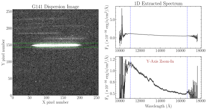
Figure 2: Left: G141 grism observation of NLTT5306 system. The brightest horizontal line, around Y=150 and between the green dashed lines, is the grism spectrum of NLTT5306. For transparency, this image shows the data before cosmic ray removal and includes bad pixels that are corrected before aXe performs spectral extraction (see Section 4). Top Right: An example of a 1D spectrum from axecore using a 4 pixel radius extraction window. Spectra inside the vertical, blue dashed lines denote the wavelengths used for science, approximately 1.1 to 1.67 $\mu$m. Bottom Right: Same as top left, except the y-axis has been zoomed in to highlight the shape of the science spectrum. The exceptionally high signal-to-noise spectra from HST WFC3 allowed us study the system in remarkable detail.

3 Observations

As presented in Table 2, NLTT5306 was observed over 2 visits of 3 orbits each on September 3rd and 4th, 2020 with Hubble Space Telescope (HST) using the WFC3/IR/G141 grism as part of HST program GO-15947 (PI: Apai). Each visit lasted approximately 236 minutes with a $\sim$797 minute gap between the end of Visit 1 and the start of Visit 2. The observations were scheduled this way to provide near-complete orbital and rotational phase coverage for this system, since the orbital period of NLTT5306 was very close to that of HST.

At the beginning of each orbit, two direct images were obtained for wavelength calibration using the F132N filter, a 256$\times$256 subarray setup, and the GRISM256 aperture. After direct images, each orbit acquired eight spectroscopic exposures in “Staring mode” of 313 s each, using the G141 grism, a 256$\times$256 subarray setup, and the GRISM256 aperture (left panel of Figure 2). This observing sequence was successfully carried out for three other WD+BD systems as part of the same HST program: WD 0137-349 (catalog ), EPIC 212235321 (catalog ) (Zhou et al., 2022), and SDSS J141126.20$+$200911.1 (Lew et al., 2022).

The third G141 observation in Orbit 6 was found to be strongly affected by a diagonal streak affecting approximately one-fourth of the image. The streak intersected with the target data and contaminated the extracted spectrum of NLTT5306. Given the 47 other high-quality frames, we excluded this frame from our subsequent analysis.

4 Data Reduction

To start the spectral extraction process, we downloaded the CalWFC3 (version 3.5.2) pipeline product flt files from the Barbara A. Mikulski Archive for Space Telescopes (MAST). We then reduced the data using an established pipeline, which combines the WFC3/IR spectroscopic software aXe (Kümmel et al., 2009) and custom Python script. This pipeline has been successful in extracting time-resolved observations of brown dwarfs (e.g., Buenzli et al., 2012; Apai et al., 2013) as well as time-resolved observations of WD+BD binaries (e.g., Zhou et al., 2022; Lew et al., 2022).

We began by organizing the data into their respective orbits, so the G141 observations in a certain orbit can have highly precise wavelength calibration using its respective direct images. We then corrected bad pixels in the G141 data, identified via the Data Quality (DQ) extension, and then linearly interpolated with adjacent good pixels. The linear interpolation was performed in the x and y direction using the median value of the neighboring four pixels on each side (i.e., up to sixteen pixels). This method worked well everywhere except for pixels that are within four pixels of the subarray edge, however, this did not effect our target data.

The F132N images and G141 data were then embedded into larger full-frame-sized (1,014$\times$1,014) arrays to allow aXe to use the standard full-frame calibration images. We median combined the full-frame F132N direct images and performed precise source extraction (Bertin & Arnouts, 1996). The output catalog file was then used by aXe for wavelength calibration.

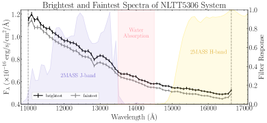
Figure 3: Science spectra of NLTT5306, after data reduction steps, including ramp effect corrections, resampling, and wavelength cutoffs (vertical dashed lines; described in Section 4). Filters profiles, shown in purple, pink, and yellow, were used to make synthetic light curves for better comparison with other observations. They were re-binned to the resolution of our data and truncated according to our wavelength cutoffs.

We prepared to run the aXe tasks, axeprep and axecore, by downloading the necessary configuration and reference files that are stored and versioned in the aXe (hstaxe) WFC3 Extraction Example Cookbook. We then ran axeprep on the G141 spectroscopic images to perform background subtraction, exposure time normalization, and gain correction. For optimal background subtraction, we performed bad pixel corrections on the master sky image, WFC3.IR.G141.sky.V1.0.fits. The process was identical to the method described above, except the locations for bad pixel corrections in the sky image were determined by the DQ extension in the first G141 observation of each orbit. Finally, we extracted the 1D spectra with axecore using a four pixel radius extraction window. Examples of an extracted 1D spectrum are shown in the right-hand panels of Figure 2.

The data exhibited signs of the instrumental systematic known as “ramp effect”, predominantly caused by electron charge-trapping and delayed release in the detector. We corrected for this effect by fitting a RECTE ramp-profile model (Zhou et al., 2017) to the uncorrected broadband light curve. The model created the ramp profile based on eight parameters. Values for the six fixed parameters controlling trapping processes, E_tot, $\eta$, and $\tau$, for both slow and fast populations were slightly updated from Zhou et al. (2017) and presented in Table 3. The two free parameters, E_0,s and E_0,f, representing the number of trapped charges at the beginning of each orbit, were found with a custom Markov Chain Monte Carlo (MCMC) performed by emcee (Foreman-Mackey et al., 2013), detailed in Section 5.1. The final ramp model was then divided out of each spectrum.

We resampled our spectra to the actual resolving power of our observations by modeling the spectral response function from each 2D stamp output by axeprep and axecore. We plotted the counts of each pixel in the direction perpendicular to the dispersion axis and fit the shape of the count curves with a Moffat profile. We then converted the Full-Width at Half-Maximum values of the Moffat profiles from pixel-space to wavelength-space using the CDELT keyword in the direct image headers. The resulting resolution of the spectra was R$\sim$130 at 14,000 Å.

The errors on the resampled spectra were calculated utilizing a method from Carnall (2017). The new error, $\sigma_{\rm{new}}$, was estimated by

$$\sigma_{\rm{new}}=\frac{\sqrt{\sum\limits^{N}_{i=1}\sigma_{i}f_{i}}}{Nd\lambda}$$ (1)

where $\sigma_{i}$ is the error on the non-resampled spectrum, $f_{i}$ is the fraction of the old bin covered by the new bin, $N$ is the total number of old bins covered by the new bin, and $d\lambda$ is the resolution of the non-resampled data, which in our case, was $\sim 47$ Å.

We ensured that we were using quality data by making wavelength cutoffs wherever the resampled flux errors were larger than two times the average error value between 13,000 and 15,000 Å. Using this condition, the resulting data on average spanned wavelengths between 11,010 to 16,670 Å (Figure 3).

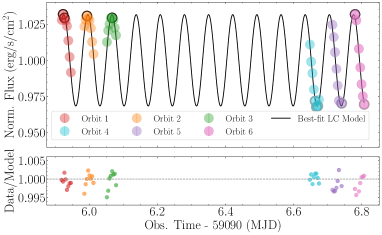
Figure 4: Normalized broadband light curve of NLTT5306, using best-fit values for RECTE and phase curve parameters, described in Section 5.1 and presented in Table 3. Using this approach, we found that a 1st-order phase curve adequately represented the data, bringing the residuals down below 0.5%. Five brightest and faintest flux values are circled in black and gray, respectively.

5 Light Curve Analysis

5.1 Best-fit Light Curve and RECTE Parameters

For this data set, we simultaneously fit RECTE parameters (E_0,s and E_0,f) and phase curve parameters. The number of phase curve parameters varied from three to five, depending on the order of the sine curve. The period ($P$) and amplitudes ($a_{k}$ and $b_{k}$) are free parameters, following methodology from Zhou et al. (2022). Basically, we treated the phase curves as a Fourier series, i.e., a combination of sinusoidal functions,

$$F(t)=1+\sum_{k}a_{k}\sin(k\frac{2\pi t}{P})+b_{k}\cos(k\frac{2\pi t}{P}),$$ (2)

where $F(t)$ is the phase curve as a function of observation time, $P$ is the period, $a_{k}$ and $b_{k}$ are the amplitudes for sine and cosine, and $k$ is the order of the sinusoidal function. So, for a 1st-order phase curve, the number of fitting parameters for the phase curve is three ($P$, $a_{1}$, and $b_{1}$), whereas this number increases to five for a 2nd-order phase curve ($P$, $a_{1}$, $b_{1}$, $a_{2}$, and $b_{2}$). Amplitudes were calculated following Equation (2) in Zhou et al. (2022), defined as: amp${}_{k}=\sqrt{a_{k}^{2}+b_{k}^{2}}$.

Table 3: Updated RECTE Parameters

Parameter	Value	Parameter	Value
Fixed Model Values
$E_{\rm{f,tot}}$	225.7	$E_{\rm{s,tot}}$	2192
$\eta_{\rm{f}}$	0.0116	$\eta_{\rm{s}}$	0.02075
$\tau_{\rm{f}}$	3344	$\tau_{\rm{s}}$	16,300
Best-fit MCMC Values
$E_{\rm{f,0}}$(1)	4.95 $\pm$ 0.04	$E_{\rm{s,0}}$(1)	0.01 $\pm$ 0.00
$E_{\rm{f,0}}$(2)	50.24 $\pm$ 0.09	$E_{\rm{s,0}}$(2)	500.16 $\pm$ 0.04

Note. — Model parameters for the RECTE ramp-profile model. In the top section, these values were treated as globally fixed for both the fast and slow populations. In the bottom section, these values represent the number of trapped charges at the beginning of each orbit and were allowed to vary in the MCMC run. We treated the two visits separately, where Visit 1 denoted as (1) and Visit 2 denoted as (2).

When finding the RECTE parameters, we fit the two visits separately, adding four free parameters in our light curve model. The two visits are separated by over 8 HST orbits, during which the charge trap status was not traceable and cannot be modeled by RECTE. Therefore, separately fitting the initial trapped charges are necessary and significantly reduces the ramp effect systematics.

To summarize the custom MCMC function, we first started by applying the RECTE parameters to the separate visits. We then created a broadband light curve from the RECTE-corrected spectra, normalized the light curve to the mean value between the 5 brightest and faintest points, and then created a phase curve model. Lastly, we calculated a likelihood value between the normalized light curve and model phase curve. The likelihood function was:

$$\rm{ln}(\mathcal{L})=\sum-0.5\left(\frac{O-M}{\sigma_{O}}\right)^{2}-\rm{ln}\left(\sqrt{2\pi\sigma_{O}^{2}}\right)$$ (3)

where O is the derived phase curve from spectral observations, M is the phase curve model, and $\sigma_{\rm{O}}$ is the error after integrating over wavelength. This process was repeated for an MCMC chain of $N_{\rm{Steps}}$=5,000 and $N_{\rm{Walkers}}$=2$\times N_{\rm{parameters}}$.

At the end, the best-fit values and uncertainties were derived from the chains after a burn-in of 250 Best-fit values for the RECTE parameters are presented in Table 3. In Figure 4, we present the final normalized broadband light curve, corrected for ramp effect, along with the best-fit phase curve model. Using this simultaneous MCMC approach, we were able to achieve residuals of less than 0.5% between the data and model. From our trials, we found that a 1st-order Fourier series model adequately represented the data, with little to no improvement in the $\chi^{2}$ fits when using a 2nd-order model. Additionally, this proves the power of the physically-motivated ramp-effect model RECTE.

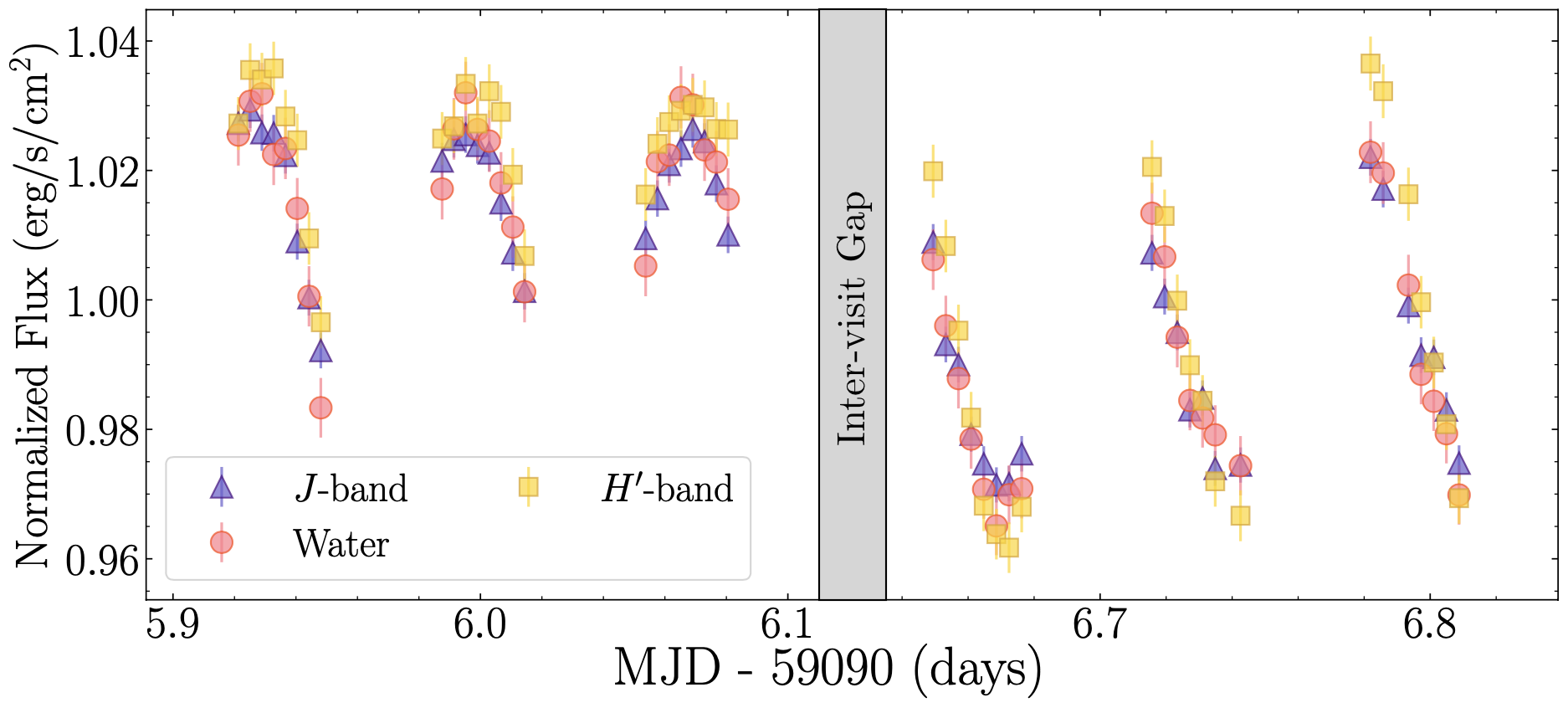
Figure 5: Normalized synthetic light curves from the 2MASS $J$-, Water Absorption, and 2MASS $H^{\prime}$-bands, integrated between 1.1 - 1.35, 1.35 - 1.45, and 1.5 - 1.67 microns, respectively. Our observations covered $\sim$6.1 periods of the NLTT5306.

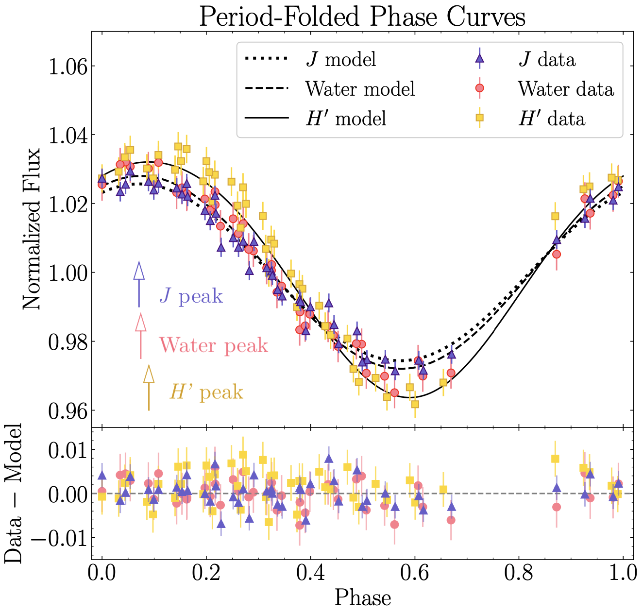
Figure 6: Phase-folded light curves in the $J$ (indigo triangle), Water (pink circle), and $H^{\prime}$ (golden square) bands along with best-fit phase curves as dashed, dotted, and solid lines, respectively. The peak of each filter is shown by arrows and labeled in the same color as the filter data. A phase of 0 here corresponds to first HST observation. For the phase curve models, we checked for a dependence on HST orbit and found none. In this figure, we observe a notable phase shift and higher amplitude in the $H^{\prime}$ filter phase curve relative to the $J$- and Water bands.

5.2 Synthetic Light Curves

To visualize and study intensity changes in a way that is easily comparable to similar analyses in other studies (e.g., Buenzli et al., 2012), we derived synthetic light curves from the spectral observations. To create the synthetic $J$-band light curve, we convolved our spectra with the Two-Micron All Sky Survey (2MASS) $J$-band transmission filter from the 2MASS All-Sky Data Release (Skrutskie et al., 2006) across a wavelength range from 11,000 Å to 13,500 Å. We then integrated over these wavelengths and normalized by the mean flux. The same process was used to create the synthetic $H^{\prime}$-band light curve, except we could not use the full wavelength range of the 2MASS $H$-band, since it extended beyond 16,700 Å. Therefore, we created an $H^{\prime}$-band light curve by integrating over 15,000 - 16,700 Å. Finally, water absorption centered around $\sim$14,000 Å is an important feature in atmospheric studies, so we also created a Water light curve by simply integrating from 13,500 to 14,500 Å. The resulting synthetic light curves are presented in Figure 5.

Table 4: Phase Curve Parameters for synthetic $J$, Water, and $H^{\prime}$-band Light Curves

Filter	Period	Amplitude
	[min]	[percent]
$J$-band	101.88$\pm$0.06	5.131$\pm$0.43
Water	101.89$\pm$0.08	5.592$\pm$0.70
$H^{\prime}$-band	101.92$\pm$0.02	6.990$\pm$0.31

In real atmospheres, different wavelengths tend to probe different pressures (e.g., Buenzli et al., 2012; Yang et al., 2016) due to varying gas and dust opacities. Therefore, comparison of the light curves allows us to compare the brightness distribution in different atmospheric layers. For our three synthetic light curves, $J$-, Water, and $H^{\prime}$-band, we created phase curve models to quantify any similarities or differences that could indicate pressure-dependent structure and dynamics. The models were created using a similar approach as described in Section 5.1, except this time we did not need to correct for ramp effect, since ramp effect was already corrected for. Therefore, we only included phase curve parameters ($P$, $a_{k}$, and $b_{k}$) in this iteration of the MCMC function.

When fitting light curves for the $J$-, Water, and $H^{\prime}$-band filters, we included higher-order models for comparison of $\chi^{2}$ values (i.e., $k$=1, 2 and 4 in Equation 2), and found that the $J$- and Water band light curves were well fit $k$=1 models, whereas the $H^{\prime}$-band light curve was better fit by a combination of $k$=1,2 models. One explanation for the $H^{\prime}$-band light curve preferring a 2nd-order combination model, resulting in a broader peak and a narrower trough, could be a longitudinally confined area of flux emission (e.g., Zhou et al., 2022), although it is not clear why the other filters would not show the same signature. The best-fit periods for the $J$-, Water, and $H^{\prime}$-bands were 101.88$\pm$0.06 min, 101.89$\pm$0.08 min, and 101.92$\pm$0.02 min, respectively. The corresponding modulation amplitudes were 5.13$\pm$0.43 percent, 5.59$\pm$0.70 percent, and 6.99$\pm$0.31 percent. These values can also be found in Table 4. The period-folded data and phase curve model for each filter are presented in Figure 6.

From Figure 6, we noticed a relative phase offset between the $H^{\prime}$-band and the other light curves, highlighted by the horizontal offset between vertical arrows in Figure 6, which represent the peaks of each filter. We calculated the difference between the peaks for each light curve and found $H^{\prime}-J$ = 6.80$\pm$0.03^∘, $H^{\prime}-$Water = 5.61$\pm$0.03^∘, and Water$-J$ = 1.19$\pm$0.01^∘. Additionally, we calculated the amplitude difference between the $H^{\prime}$-band and other synthetic light curves to be over one percent, suggesting greater variability in flux at the pressures probed by the $H^{\prime}$-band wavelengths.

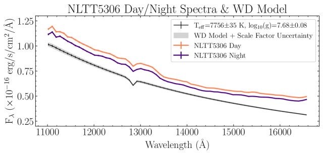
Figure 7: The day- (orange) and night-side (purple) spectra of NLTT5306, corresponding positions A and B in Figure 1. The WD contribution is shown below in black. The uncertainties associated with the WD model, i.e. uncertainty in effective temperature and surface gravity, are shown as the black errorbars, whereas the total uncertainty, which includes uncertainty in scale factor (via uncertainty in distance to the system and white dwarf radius), is shown as the gray shaded region. From this figure, we can see that the contribution of the brown dwarf is approximately 20% of the flux in the NIR.

Absolute phase offsets relative to eclipse would be useful for testing for evidence for any prograde (eastward) or retrograde (westward) hot spot shifts in the atmosphere of NLTT5306B. Doing so requires comparing the orbital phase of the brown dwarf to the phase of the maximum brightness. In the absence of an eclipse (which would provide orbital phase information), this could be achieved using precise radial velocity measurements. Longstaff et al. (2019) calculated a radial velocity ephemeris using XSHOOTER data from 2014. However, the uncertainty on the period and orbital phase propagated to the time of our observations is too large ($\sim$10.1 hours or $\sim$6$\times$ the rotational period) to allow the precise determination of absolute phase offsets. Thus, current data is insufficient to test for a potential hotspot offset. In future observations, we encourage contemporaneous radial velocity and spectroscopic measurements.

5.3 Investigating Phase Offsets and
Modulation Amplitudes

Motivated by the $>$5 degree relative phase offsets and $>$1% amplitude differences between the $H^{\prime}$-band and the other synthetic light curves, we performed a more detailed analysis in an effort to pinpoint which wavelengths, and therefore which pressures, contributed most to these differences. Methods for this investigation are described in Appendix Section A, with the results presented here.

In both the 1st and 2nd order models, the highest amplitudes reach $\sim$8%, coming from two wavelength regions around 15,450 and 16,250 Å, which would both fall into $H^{\prime}$-band synthetic light curve. Following the $\sim$8% peaks, there is a $\sim$7% peak around 12,900 Å, just inside the wavelength range of the $J$-band synthetic light curve. Phase offsets in the 1st order phase curve models (Figure 22) mostly follow the same shape as the modulation amplitudes curve, except for the longer wavelength $H^{\prime}$-band region, where the phase offsets appear to stay constant. In the 2nd order phase curve models, (Figure 23), the phase offsets again follow the shape of the amplitude curve, except at the three wavelength regions where amplitudes exceed 7%. Here, the offsets appear to be inversely correlated to the amplitudes peaks. The complex, highly wavelength-dependent behavior of the phase offsets and amplitudes are not seen in 3D models of irradiated brown dwarf atmospheres.

6 Rotational Phase-Resolved Spectra of the Brown Dwarf NLTT5306B

6.1 Subtracting the White Dwarf Contribution

In order to obtain the phase-resolved spectra of the brown dwarf, it was first necessary to remove the contribution of the white dwarf from the observed WD+BD spectra. Since this system is unresolved and does not eclipse, it was not possible to get a spectrum of the white dwarf alone. Thus, we modeled the white dwarf spectrum using a model grid for pure-hydrogen atmosphere WDs from Koester (2010), which used two free parameters, $T_{\rm{eff}}$ and log($g$). We adopted the published white dwarf values for these parameters (Table 1) and bi-linearly interpolated along the Koester (2010) model grid. To account for uncertainty in the published values of $T_{\rm{eff,WD}}$ and log($g$)_WD, we created 10,000 models for different values of temperature and surface gravity, sampled from Gaussian distributions with means of 7756 K and 7.68 cm s^-2 and standard deviations of 35 K and 0.08 cm s^-2, respectively. We then found the uncertainty of the WD model by measuring the FWHM of the fluxes from 10,000 models at each wavelength, seen as a solid black line with errorbars in Figure 7.

There was also uncertainty in the ‘scale factor’ used to scale the model flux into what the expected observed flux would have been. To account for this noise source, we multiplied the flux at each wavelength by the scale factor, $\big{(}\frac{R_{\rm{WD}}}{D}\big{)}^{2}$, adopting published values and propagating uncertainties for $R_{\rm{WD}}$, white dwarf radius, and $D$, distance to the system. Therefore, the total error in the WD model comes from two sources, shown as the gray shaded region in Figure 7.

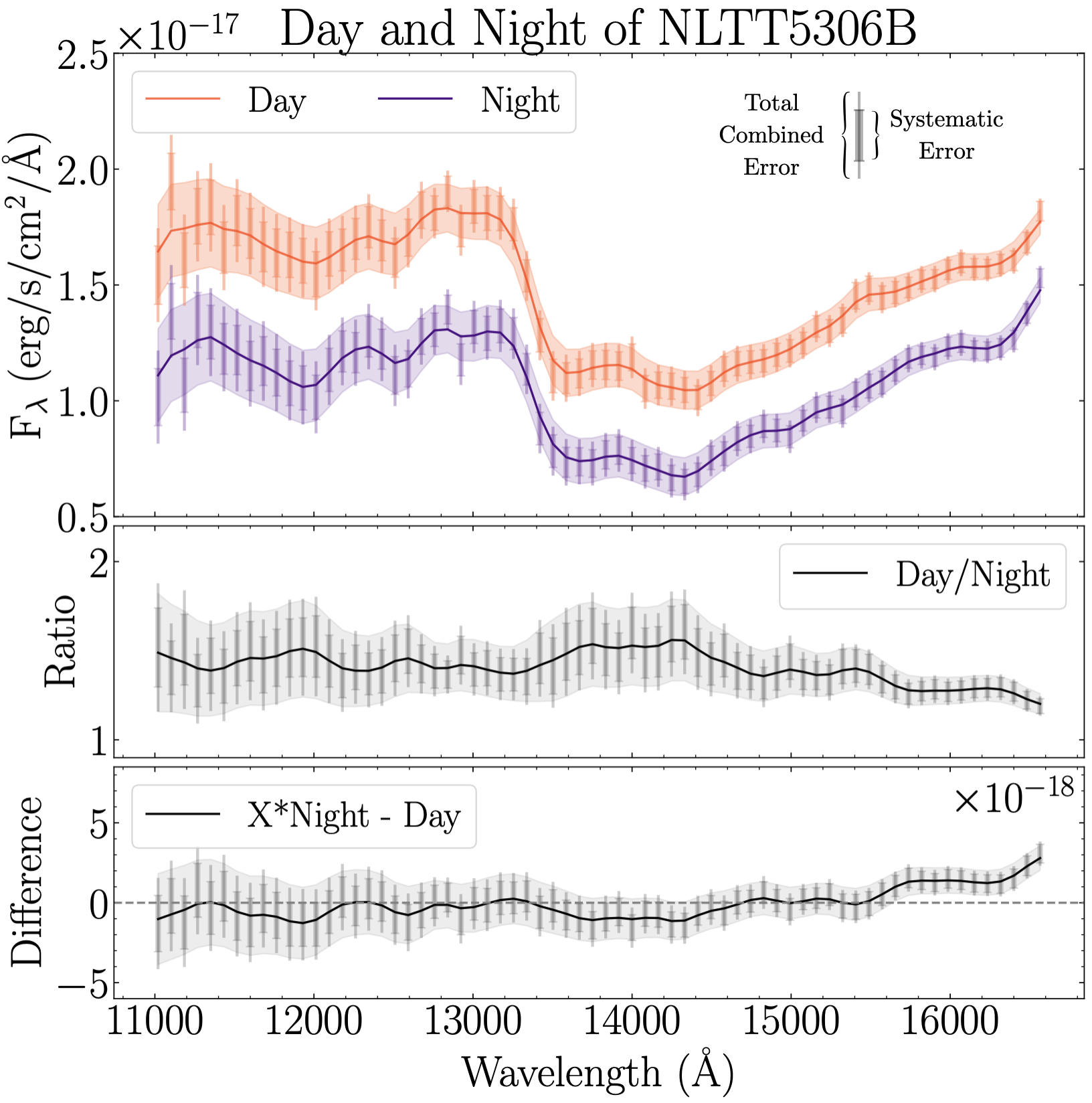
Figure 8: Top: The Day/Night spectra of NLTT5306B. Systematic uncertainties and total combined errors are shown as thin and thick erorrbars, respectively. Solid lines and shaded regions are observations and total uncertainties convolved with a Gaussian kernel with a width equal to the spectral resolution of our observations. Middle: The ratio between the day- and night-side spectra. Interestingly, while the overall ratio between the day and night spectra are roughly constant, there is a noticeable bump near the water absorption feature. Bottom: The difference between the day- and night-side spectra, where the night-side spectrum has been vertically scaled by X=1.37, such that the average of the difference is equal to zero.

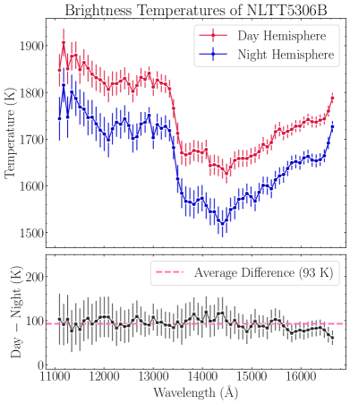
Figure 9: Top: The day and night brightness temperatures of NLTT5306B, calculated by the solving the Planck equation for $T_{\rm{B}}$ at each wavelength. Errors here depict 1$\sigma$ uncertainties. Bottom: The difference in brightness temperatures between the day- and night-sides, along with the average difference over all wavelengths, plotted as a pink dashed line. Remarkably, the difference in brightness temperatures is nearly constant across the 1.1$-$1.67$\mu$m range.

6.2 Extracting Day/Night Spectra of NLTT5306B

Thanks to our observations having near-complete phase coverage and very high data quality, we were able to confidently isolate and compare our analyses of the “Day” and “Night” sides of NLTT5306B. To further improve the signal-to-noise ratio, minimize any spectral variations, and secure the precision of the derived day/night spectra, we took the median of the five brightest and faintest spectra across all orbits and designated them as the day and night spectra. The corresponding brightest and faintest light curve points are circled in black and gray in Figure 4. The NLTT5306 day- and night-side spectra produced with this method are shown in Figure 7.

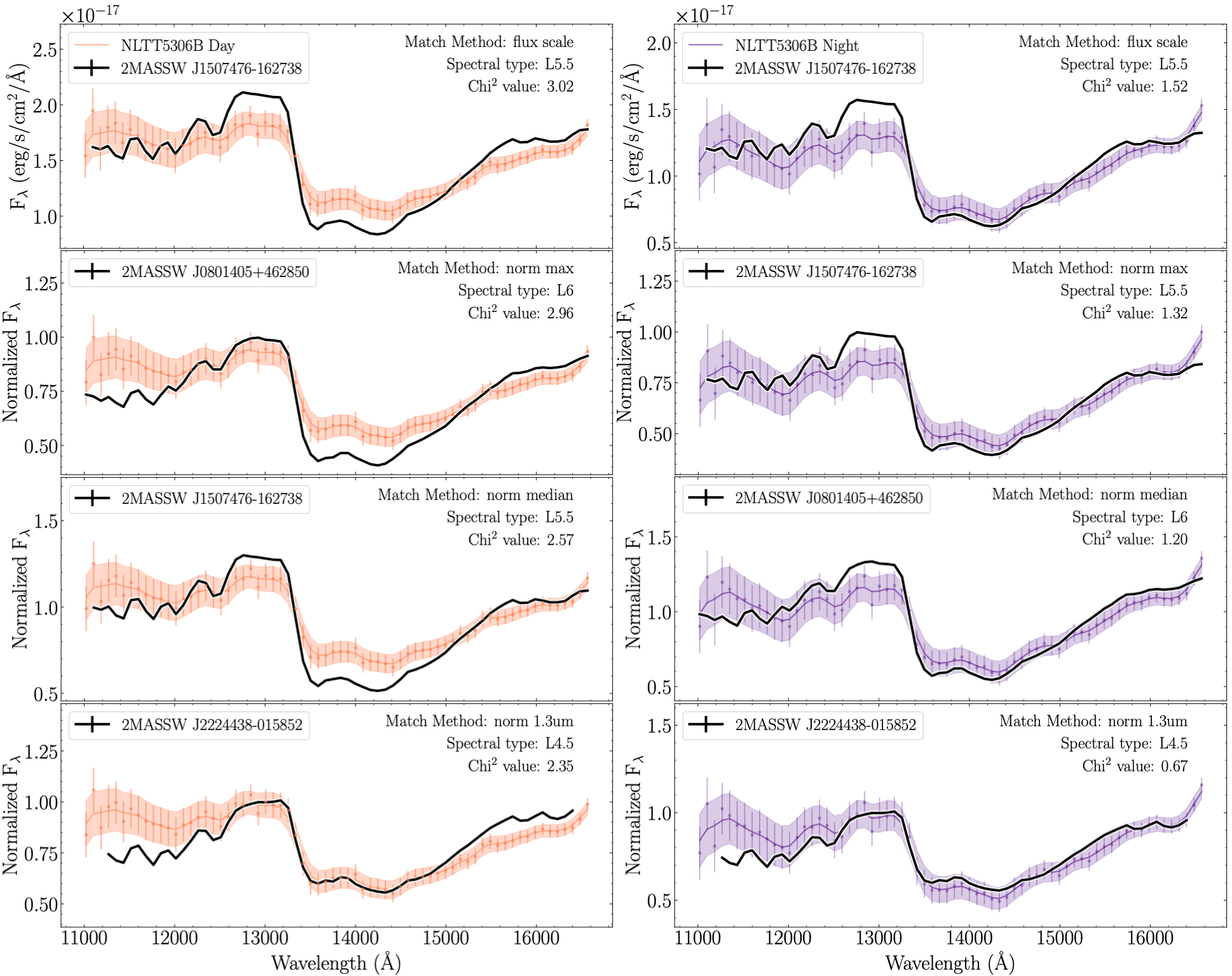
Figure 10: Comparison of the day- and night-sides of NLTT5306B with their closest matching Cloud Atlas spectra. Plotting conventions for the observed brown dwarf spectra are the same as Figure 8. Left column shows the day-side comparison (orange) whereas the right column shows the night-side (purple). Each row depicts a specific matching method. From top to bottom, they are: (1) Flux scaling to photometry, (2) normalizing to maximum flux value, (3) normalizing to median flux value, and (4) normalizing to flux at 13,000 Å.

Once the WD contribution was modeled and subtracted, we extracted the BD component for further atmospheric investigation. The isolated day- and night-side spectra are presented in the top panel of Figure 8. The day-side is 40% brighter than the night-side, on average, seen in the middle portion of Figure 8. We attempted to rule out the possibility that the day-side is simply a direct scaling of the night-side by multiplying the night spectrum by a constant $X$=1.37 and then subtracting the day-side. From the non-constant shape of the difference curve, bottom portion of Figure 8, we found that the day-night-side difference is not just in intensity, but also in their spectral features.

6.3 Day/Night Brightness Temperatures

In the atmospheres of stellar companions, the combination of internal heat flux, profile of net absorbed stellar flux, and opacity structure control the thermal structure (Marley & Robinson, 2015a). To study this structure in detail, we derived brightness temperatures at each wavelength, defined as the temperature at which a blackbody would emit as much specific intensity as the observed value. When coupled with a Pressure-Temperature (P-T) profile, brightness temperature is a useful proxy to map the relative pressure regions probed by each wavelength, which in turn reveals the vertical structure of the atmosphere at each observed phase. Using Planck equation and published values for brown dwarf radius and distance to the system (Table 1), we calculated brightness temperatures versus wavelength for both the day-and night-sides of NLTT5306B, shown in Figure 9.

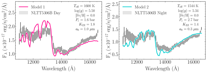
Figure 11: Day (Left) and night (Right) spectra of NLTT5306B with best-fitting models from the cloudy, non-irradiated model grid that included cloud opacities from Brock et al. (2021). Model parameters are labeled towards the right side of each figure. From these fits, we conclude that NLTT5306B most likely has an internal temperature around 1550 - 1600 K.

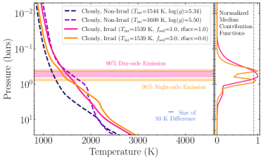
Figure 14: Left: Pressure vs. temperature profiles for the models shown in Figures 11 (dashed lines) and 13 (solid lines). The size of the 93 K temperature difference seen in the observed day and night brightness temperatures (e.g. Figure 9) is shown as a blue bar in the bottom right. Right: Corresponding normalized contribution functions to the irradiated models. A gray dashed line at 0.9 depicts the pressure regions where $\geq$90% of atmospheric emission originates for both models, also shown as shaded regions in the left panel.

In both hemispheres, the brightness temperatures showed strong wavelength dependence with temperatures that ranged between 1500 and 1900 K, with the lowest temperatures located around the water absorption band. These temperatures fall within the range where silicate clouds are expected to be an important opacity source (Ackerman & Marley, 2001). Since both the day and night hemispheres fall within this temperature range, it is likely that silicate clouds are present above the photosphere at all phases. The brightness temperatures also exhibited a nearly constant temperature difference of 93 K between day and night, further supporting the interpretation that both hemispheres possess similar gas-phase abundances and opacity sources. This small temperature difference was also seen in the P-T profiles presented in Figure 14.

7 Comparison to Field Brown Dwarfs

7.1 Cloud Atlas Spectral Library

Next, to understand the impact of external irradiation on the atmosphere of NLTT5306B and brown dwarf atmospheres in general, we compare our derived irradiated brown dwarf spectra to a spectral library of non-irradiated brown dwarfs, also observed with the same telescope and instrument setup. Specifically, the Cloud Atlas Hubble Space Telescope Large Treasury program (PI: Apai) has, among other results, published a comprehensive, high-quality spectral library of 76 HST/WFC3/NIR/G141 spectra. In order to investigate the differences between field brown dwarfs and irradiated brown dwarfs, we first sought to find a best-match spectral type from this library. Of the 76 Cloud Atlas spectra, 66 are spectra of L, T, and Y dwarfs (see Table 1 in Manjavacas et al. 2019). We were able to use 53 of these spectra, since data for CD$-$352722b is missing from the downloadable tar.gz file and 13 others were excluded to ensure a high-quality data set with well-understood brown dwarf spectral types. The 13 spectra we excluded were: (1) eight objects were considered Planetary-Mass Companions (see Table 3 in Manjavacas et al. (2019)), (2) three objects with two reported spectral types, and (3) one object with a spectral type of Y0pec.

Since there are uncertainties in many of the physical parameters we would use to find a best-match spectrum for the day- and night-sides of NLTT5306B, e.g. radius, effective temperature, and distance, we attempted to circumvent such uncertainties by using four different matching methods, three of which are close to being scale factor and temperature independent. The four methods, shown in Figure 10 for both the day and night-sides, included normalizing to the maximum flux value in wavelength range of our observations, normalizing to the median flux value, normalizing to the flux value at 13,000 Å, and flux scaling to match photometry. The procedure for flux scaling is described in Appendix Section B.

Of the four matching methods used for the Cloud Atlas spectral library, normalizing to the flux value at 13,000 Å provided the closest match of spectral features. This could be expected, since 13,000 Å probes the highest pressure among the wavelengths considered here, and thus should be less affected by irradiation. For the day-side of NLTT5306B, the closest Cloud Atlas spectrum, with a $\chi^{2}$=2.35 was 2MASSW J2224438-015852, an L4.5 dwarf (Dupuy & Liu, 2012). This brown dwarf was also the best-match for the night-side of NLTT5306B, with a $\chi^{2}$ value of 0.67. 2MASSW J2224438-015852 is known to have a significant silicate cloud feature around 10 $\mu$m (Cushing et al., 2006), supporting our later interpretation of NLTT5306B as having significant cloud coverage.

8 Non-Irradiated Brown Dwarf Models

8.1 Brock Model Grid

In an effort to provide a baseline for the expected condensate clouds, we started our modeling procedure by comparing the observed day-side and night-side spectra of NLTT5306B to non-irradiated models that included cloud opacity from Brock et al. (2021). These models had much the same setup as described in Section 9.1, but included the opacity from a variety of important condensate species, including silicates, corundum, iron, and many more (Allard et al., 2001). The vertical extent of the clouds was determined by a vertical mixing parameter ($K_{\rm{zz}}$) and a $P_{\rm{c}}$ parameter, which describes the pressure at which the cloud particle number density begins to decrease exponentially. The mean particle size of the log-normal distribution of grain sizes was varied between 0.125 and 10 $\mu$m.

To find a best fit model for day and night, we applied a scale factor, $\big{(}\frac{R_{\rm{BD}}}{D}\big{)}^{2}$, to all models and then calculated the $\chi^{2}$ value between each model and the day- and night-side spectra for the brown dwarf. We determined the best match for each side by finding the smallest $\chi^{2}$ value. Figure 11 shows the best-fit cloudy, non irradiated models from the Brock model grid to the extracted day and night spectra of NLTT5306B, which are listed in full in Table 5. The models had $T_{\rm{eff}}$ between 1544 $-$ 1600 K and surface gravity, log($g$), values between 5.34 $-$ 5.50, for night and day, respectively. Along with the Cloud Atlas fits, we used the parameters of these models as a baseline for the brown dwarf parameters that the irradiated models would start from. As this system is not eclipsing, we chose to approximate the night-side of NLTT5306B as the closest estimate for a non-irradiated atmosphere. Thus, we concluded that the internal temperature of NLTT5306B was most likely between 1544 and 1600 K, meaning that without external irradiation, we could expect the dominant opacity sources to be H₂O, CO, and silicate grains, which are predicted for temperatures above 1500 K (Burrows et al., 2001).

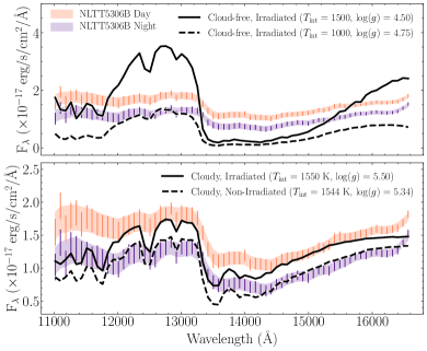
Figure 12: Top: Comparison of day (orange) and night (purple) extracted spectra of NLTT5306B with best-fit cloud-free, irradiated models from the Lothringer Model Grid (described in Section 9.1). Neither model was a good match to the data. Bottom: Same as top panel, except with cloudy models where both irradiated and non-irradiated were considered. The spectra of NLTT5306B are more muted than the models predict, however it is clear that they prefer cloudy over cloud-free models from this model grid.

9 Irradiated Brown Dwarf Models

9.1 Lothringer Model Grid

We compared the observations to a grid of cloud-free PHOENIX irradiated brown dwarf atmosphere models, similar to those described in Lothringer & Casewell (2020). The models are calculated from 10 to 10⁷ Å with 1-2 Å sampling up to 5 $\mu$m, with coarser sampling at wavelengths longer than 5 $\mu$m. We varied internal temperature ($T_{\rm{int}}$=1000, 1500, 2000, 2500 K), surface gravity ($\log g$ = 4.5, 4.75, 5.0), metallicity ([Fe/H] = -0.5, 0.0, 0.5), and heat redistribution ($f$ = 0.125, 0.25, 0.5, where 0.5 implies day-side redistribution, 0.25 implies full heat redistribution, and 0.125 implies full redistribution with a non-zero albedo). The final effective temperature of the brown dwarf is a combination of the internal temperature ($T_{\rm{int}}$ — temperature associated with internal heat flux) and temperature caused by external irradiation ($T_{\rm{irr}}$ — see Equation 1 in Lothringer & Casewell (2020)), like so:

$$T_{\rm{eff}}=\big{(}T_{\rm{int}}^{4}+T_{\rm{irr}}^{4}\big{)}^{1/4}$$ (4)

In models with no external irradiation, the effective temperature is the same as the internal temperature. The brown dwarf models use the BT2 H₂O line list (Barber et al., 2006), as well as HITRAN 2008 for other major molecular absorbers (Rothman et al., 2009) and Kurucz data for atomic species (Kurucz & Bell, 1995). We used the Koester (2010) white dwarf spectrum closest to NLTT5306A’s fundamental parameters to irradiate the brown dwarf atmosphere.

Figure 12 shows the day and night spectra of NLTT5306B with four different models from the Lothringer model grids: two cloud-free and irradiated, one cloudy and irradiated, and one cloudy and non-irradiated. For the cloud-free and irradiated model grid, we used the same matching method as described in Section 8, where we applied a scale factor and compared $\chi^{2}$ values. The resulting best matches, with all of their free parameters, are presented in Table 5. For the day-side, a $T_{\rm{eff}}$ = 1500 K, log($g$) = 4.50 model was the best match. However, the model’s peak flux was almost two times higher than the observed peak flux and the model’s water absorption feature was also much deeper. The best-fit for the night-side was a $T_{\rm{eff}}$ = 1000 K, log($g$) = 4.75 model. This model better matched the peak flux of the extracted night-side spectrum, although the water absorption feature was again too deep.

The irradiated model grid was cloud-free, so poor model fits are not so surprising since we expect the atmosphere of NLTT5306B to be cloudy. As such, we also ran irradiated versions of the best-fitting Brock models, which included clouds, shown in the bottom panel of Figure 12. With this method, we found that the best match for the day-side spectrum was a cloudy, irradiated model with $T_{\rm{eff}}$ = 1550 K and log($g$) = 5.50. For the night-side, a cloudy, non-irradiated model with $T_{\rm{eff}}$ = 1544 K and log($g$) = 5.34 provided the closest fit overall. This night-side match is the same model seen on the right side of Figure 11.

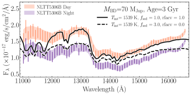
Figure 13: Best-fit models from the Sonora model grid compared with extracted day and night spectra of NLTT5306B. The brown dwarf mass, age, and internal temperature are the same for both models, with the sedimentation and recirculation parameters ($f_{\rm{sed}}$ and rfacv) driving the difference between the two models.

9.2 Sonora Model Grid

We compared the observations to several forward models of both cloudless and cloudy atmospheres in 1D computed using the irradiated giant planet atmospheres code of Marley et al. (1999) which generates an atmospheric radiative-convective equilibrium thermal profile based on given object properties, based on the methods of McKay et al. (1989) (see also Marley & Robinson, 2015b). We follow the same process employed by Mayorga et al. (2019) and Lew et al. (2022), which we summarize here.

We first computed cloud free models assuming an internal heat flux, parameterized as above by a $T_{\rm int}$, as determined by the Marley et al. (2018) evolution grid and an age. We assumed chemical equilibrium and solar abundances. We did not include TiO and VO opacity in our calculation as these species are expected to be condensed into grains at these temperatures.

The high $T_{\rm{eff}}$ of the white dwarf primary (in excess of 7500 K) results in a substantial fraction of its radiation being emitted blueward of the shortest atmosphere model spectral interval at $0.25~{}\mu$m. Because of the dearth of available UV opacities for gaseous absorbers the model cannot be straightforwardly extended to shorter wavelengths. To approximately account for the influence of the blue white dwarf flux on the model atmospheric structure, we applied a rudimentary correction by integrating the white dwarf flux short-ward of the bluest bin in the atmosphere model and added it uniformly to all of the spectral bins short-wards of 0.4 $\mu$m (to avoid the potassium absorption lines). In essence this treats the bluest incident flux as having the same disposition as flux in the interval of 0.25 to $0.40~{}\mu$m.

To model the white dwarf primary we selected a Koester (2010) model at 7750 K and log($g$)=7.5 as the stellar host. We assumed a recirculation efficiency, rfacv, of 1 to represent a day-side average model rather than of 0.5 to represent a global average. We used PICASO (Batalha et al., 2019) to generate the combined reflected and thermal emission spectra.

We also computed self-consistent cloudy 1D models for each companion allowing the following gas species to condense as appropriate: NH₃, H₂O, KCl, ZnS, Na2S, MnS, Cr, MgSiO₃, Fe, Al₂O₃ (Morley et al., 2012; Marley et al., 2013). The particle size and vertical extent of the cloud layer was controlled by setting the cloud sedimentation efficiency parameter, $f_{\rm{sed}}$ (Ackerman & Marley, 2001). A small $f_{\rm{sed}}$ yields tall lofted clouds of small particles while a large $f_{\rm{sed}}$ produces a vertically thin cloud with generally larger particles. Studies of brown dwarfs and Jupiter-like planets indicate that the appropriate $f_{\rm{sed}}$ to model clouds should be roughly 1–3 (Stephens et al., 2009; Ackerman & Marley, 2001). As with the cloudless models the profiles are iterated until a self-consistent radiative-convective equilibrium profile is obtained. We explored cloud free atmospheres and $f_{\rm{sed}}$ = {3.0 and 1.0}.

We first modeled the day-side using the given mass for the brown dwarf and age from Steele et al. (2013) (52 M_Jup and 5 Gyr). In general, we found that these models were unable to provide a reasonable match to the observed spectra as they were far too cool. Our next step was to explore models with younger ages, which would increase their internal heat fluxes closer to those observed. Models with higher internal temperatures better matched the feature near 1.4 $\mu$m but, in general, lead to an over-prediction of the flux at all other wavelengths that could not be remedied by changing the cloud properties to sufficiently mute the features without masking them entirely. Varying the surface gravity of a model can also reduce the scale heights of features. Therefore, we explored models of 5 Gyr and 3 Gyr with masses ranging from 50-80 M_Jup. We found that the best match of the observed spectrum was fit by a model with an internal temperature of 1539 K (3 Gyr, 70 M_Jup) and $f_{\rm sed}$ = 1.0, shown in Figure 13 and listed in Table 5.

Using these best-fit parameters of 3 Gyr and 70 M_Jup, we explored recirculation efficiencies, rfacv$<$1, to match the night-side spectrum with various cloud $f_{\rm sed}$ combinations. The night-side was best fit with an rfacv=0 and $f_{\rm sed}$ = 3.0, shown in Figure 13. We found that it was difficult to match both the flux levels of both the short- and long-wavelength portions of the spectrum with the 1D model.

10 General circulation modeling
of NLTT5306B

To understand the general circulation and interpret the observed light curves of NLTT5306B, we adapted a general circulation model (GCM) appropriate for NLTT5306B. The atmospheric circulation and 3D thermal structure were simulated using the SPARC/MITgcm GCM which originated from simulating hot Jupiter atmospheres (Showman et al., 2009). The model solves the global primitive equations of dynamical meteorology that are suitable for the outer most observable layers of giant planets and brown dwarfs. Radiative heating and cooling rates in each column of the GCM are calculated using the non-grey radiative transfer model of Marley et al. (1999) that solves the two-stream radiative transfer equations and employs the correlated-k method. The correlated-k opacity tables have been updated based on the opacities used in Marley et al. (2021). We assume equilibrium chemistry in the atmosphere.

Here we introduce the specific setups of the GCM for NLTT5306B. The stellar spectra of NLTT5306 is obtained from the best fit used in Section 6.1 and the missing fluxes at lower and higher wavelengths are assumed to be blackbody radiation using the best-fit stellar temperature and radius. The temperature of the lowest model layer (at a pressure of about 130 bars) in the GCM is relaxed towards a prescribed value of 3700 K which is informed by the cloud-free Sonora grid model with a log($g\rm{)}=5$ and internal temperature of 1600 K. This boundary condition differs from previous setups of hot Jupiters (e.g., Showman et al., 2009) in which a uniform net heat flux was prescribed. Our bottom boundary condition mimics a rapid entropy mixing by vigorous interior convection, and we argue that this is more appropriate here because convection mixes the entropy (towards the uniform interior entropy) rather than heat flux and that our GCM deep layers have reached the convective zone. To deal with the convective instability, we apply a convective adjustment scheme to remove convective instability instantaneously (the implementation is described in Tan, 2022). The primary WD is much smaller than and very close to the BD companion, and we have applied a geometry correction of the WD irradiation on the BD atmosphere. A linear drag is applied at pressures larger than 50 bars to crudely represent interactions with the interior similar to that implemented in Tan (2022). The model domain extends from 150 bars to $3\times 10^{-4}$ bar with 53 vertical layers and has a cubed-sphere C64 horizontal resolution (equivalent to $256\times 128$ in longitude-latitude grid).

The global temperature map at 0.49 bar from the GCM results of NLTT5306B is shown in Figure 15 along with the horizontal wind vectors as black arrows. The most prominent feature is that the overall temperature pattern does not significantly deviate from that determined purely by the radiative transfer, meaning that circulation is inefficient to drive strong winds in the global scale to shift the temperature pattern. The day-to-night temperature variation appears to be much smaller than the global mean temperature; this is not due to dynamical heat transport but rather is because the irradiation is much weaker than the internal energy of NLTT5306B. Despite the global inactive circulation, a somewhat strong equatorial jet stream appears but is confined within a few degrees around the equator. At two sides of the equatorial jet, two meridionaly narrow hot lobes develop and are shifted westward; these are the so-called stationary Rossby lobes which are rotational response to the day-night thermal contrast. The horizontal temperature structures at other pressures are qualitatively similar to that shown in Figure 15. Such a circulation pattern is related to the rapid rotation of NLTT5306B as explained in Tan & Showman (2020) and also shown in GCM results for other BDs around WDs (Lee et al., 2020; Sainsbury-Martinez et al., 2021; Lee et al., 2022).

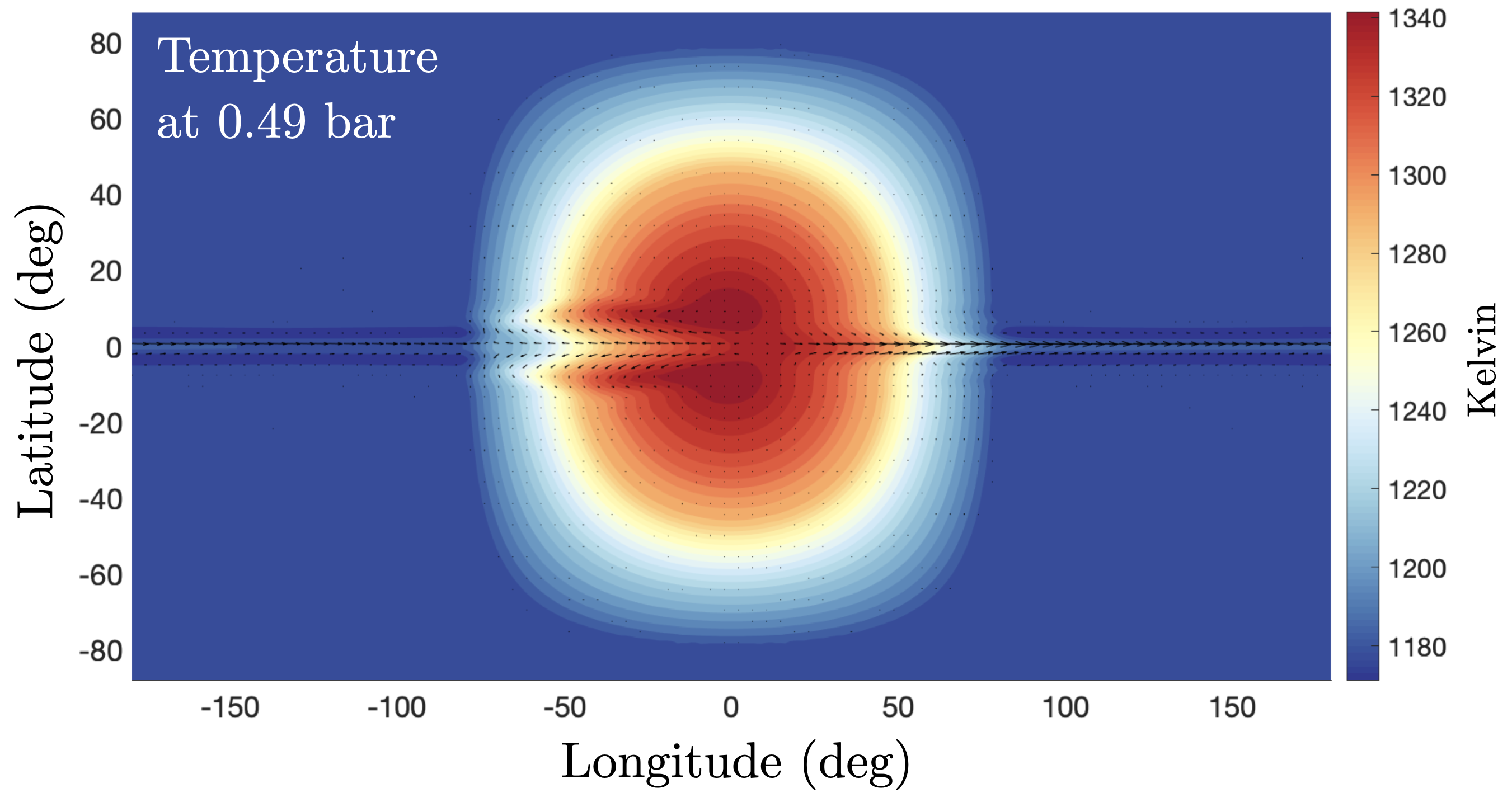
Figure 15: Temperature distribution at $P$=0.49 bar in the GCM simulation of NLTT5306B. This pressure level was chosen since it is roughly in the middle of where most of the emitting flux originates from based on Figure 14. We see an eastward jet at the equator with thin westward-shifted lobes at equator-adjacent latitudes.

Because of the globally inactive circulation, the thermal light curves from the GCM results show negligible phase offsets. The wavelength-dependent thermal phase curves were generated by feeding the time-average global temperature structure to PICASO (Batalha et al., 2019; Robbins-Blanch et al., 2022), which shared the same opacity source as our GCM and so ensured consistency between post processing and the GCM. Phase curves were created for a sample of wavelengths representative of the HST spectra, and phase curve models were fit using the same methods described in Section A. The amplitudes and relative phase offsets were calculated for every model and investigated for wavelength-dependent behavior. Unlike what it seen in the observations (e.g. Figures 6, 22, and 23), there are no relative phase offsets among the thermal phase curves from the adapted GCM. Model amplitudes were strongly dependent on wavelength (ranging from 2 to 40%), in contrast to the smaller amplitude changes seen in the observed phase curves.

Our cloud-free GCM practice suggests that the cloud-free circulation scenario cannot explain the observed light curves. This is not surprising because clouds are already shown to be essential to interpret the observed day-side and night-side spectra (see section 8 and 9). The importance of clouds and internal heat flux points to two possible improvements. The first is to consider the mechanism generating light curve variability of many isolated BDs by radiatively cloud driven circulation (Tan & Showman, 2021). The second is related to waves triggered by interactions between convection and the overlying stratified layers which could result in vertically sheared zonal flows in both isolated BDs (Showman et al., 2019; Tan, 2022) and young hot Jupiters (Lian et al., 2022). Of course, mechanisms of cloud radiative effects in hot-Jupiter-like irradiation (e.g., Roman & Rauscher, 2019; Parmentier et al., 2021; Komacek et al., 2022) would also be important when interpreting cloud models for these type of objects as irradiation is still nontrivial.

11 Discussion

11.1 System Parameters

Here we compare the newly calculated light curve period of NLTT5306 with values from previous studies. The first published period of $P$=101.88$\pm$0.02 min was determined via radial velocity (RV) observations back in 2013 by (Steele et al., 2013), 8 years before these HST observations. Longstaff et al. (2019) then constrained the period further to $P$=101.88 min $\pm$ 0.000002 ms in 2019. While 8 years is short compared the timescale of orbital decay (approximately 900 Myr; Steele et al., 2013), we might still expect to find a shorter orbital period, as this system is experiencing orbital decay on its way to becoming a cataclysmic variable.

Our best-fit broadband light curve model of NLTT5306 resulted in a period of 102.05$\pm$0.07 min, longer than the published values from Steele et al. (2013) and Longstaff et al. (2019). Including uncertainties, the value we found is just over 3$\sigma$ away from those published values. This could be due to the fact that radial velocities trace orbital motion, whereas phase curve observations trace atmospheric rotation. Zhou et al. (2022) also found a slightly longer light curve period than the radial velocity period of WD 0137. Therefore, if NLTT5306B’s atmosphere contains dynamics that exhibit local retrograde motion, like a westward traveling feature, the period measured by the phase curve can be prolonged even further. Thus, we cannot yet definitely say if the orbital period has evolved.

One system parameter that may impact our findings is the uncertain orbital inclination of NLTT5306. While precise orbital inclination was unknown, we were able narrow down the possible range of values based on observational constraints. For example, due to the lack of any observed transit in the phase curve, Buzard et al. (2022) previously estimated an upper limit of $i\leq 78.7^{\circ}\pm 0.4^{\circ}$ with the following equation:

$$i_{\rm{partial}}=90^{\circ}-\rm{sin}^{-1}\Big{(}\frac{R_{\rm{BD}}+R_{\rm{WD}}}{a}\Big{)},$$ (5)

and using the brown dwarf radius (informed by evolutionary models) of $R_{\rm{BD}}=0.095\pm 0.004$ R_⊙ (Table 1). Additionally, we used the observed radial velocity semi-amplitude and its connection to the two masses in the system, and the inclination as follows:

$$\frac{M_{2}^{3}\rm{sin}^{3}(i)}{(M_{1}+M_{2})^{2}}=\frac{PK^{3}}{2\pi G},$$ (6)

where $M_{\rm{1}}$ is white dwarf mass, $M_{\rm{2}}$ is brown dwarf mass, $i$ is inclination, $P$ is orbital period, and $K$ is semi-amplitude of radial velocity. Although the mass of the brown dwarf is not directly measured, we may use $M_{\rm{2}}$ = 75 M_Jup as a conservative upper limit. With this, solving for $i$, and adopting values from Table 1 for $M_{\rm{1}}$ and $P$, and $K_{\rm{H_{emis}}}=-49.1\pm 1.1$ km/s from Longstaff et al. (2019), we found a lower limit of $i\geq 58.0\pm 1.1$ degrees. Thus, for NLTT5306, we estimate the possible range of inclinations to be between between 58^∘ and 79^∘. In the following section (and in § 11.6), we discuss how this range of possible inclinations could impact our results.

11.2 Longitudinal Temperature Distribution

With the known observed parameters of the system, (i.e., orbital separation and temperatures and radii of both dwarfs), we constructed a simple radiative equilibrium-based temperature distribution map of NLTT5306B, shown in Figure 16. The calculation of this map consisted of a grid search among four parameters: (1) Bond albedo ($A_{B}$), which set the fraction of incident irradiation that is reflected away from the day-side, (2) irradiation redistribution fraction ($f_{\rm{irr-red}}$), which controlled how much of the non-reflected irradiation was redistributed to the night-side, (3) non-irradiated brown dwarf temperature ($T_{\rm{non-irr}}$), which set the base temperature of the brown dwarf without irradiation, and (4) Inclination ($i$), which effectively controlled how much of one hemisphere was visible when the other hemisphere was dominating the emission. The grid search process is further described in Appendix Section C.

Figure 16 shows the 2D temperature distributions from the best-fit combination of parameters: $A_{B}$ = 0.28$\pm$0.07, $f_{\rm{irr-red}}$ = 0.70$\pm$0.02, $T_{\rm{non-irr}}$ = 1260$\pm$20 K, $i$ = 78.0${}^{+1.1}_{-7.6}$ degrees. The parameters were fit to match a night-side temperature of 1500 K, informed by the night-side brightness temperature at 1.4 $\mu$m, and a day-side temperature of 1593 K, motivated by the 93 K difference seen in derived brightness temperatures between day and night (Figure 9). We note that the relatively high Bond albedo is physically consistent, given that most the incident radiation from the white dwarf is in the UV/Optical blue and the predicted global presence of silicate clouds in this atmosphere (Marley et al., 1999). Although this model is rather simple, our ability to obtain a good match to observations with physically reasonable parameters suggests that we are able to capture the fundamental processes at play. Such models are powerful in providing physical intuition and insights into the key processes within these atmospheres.

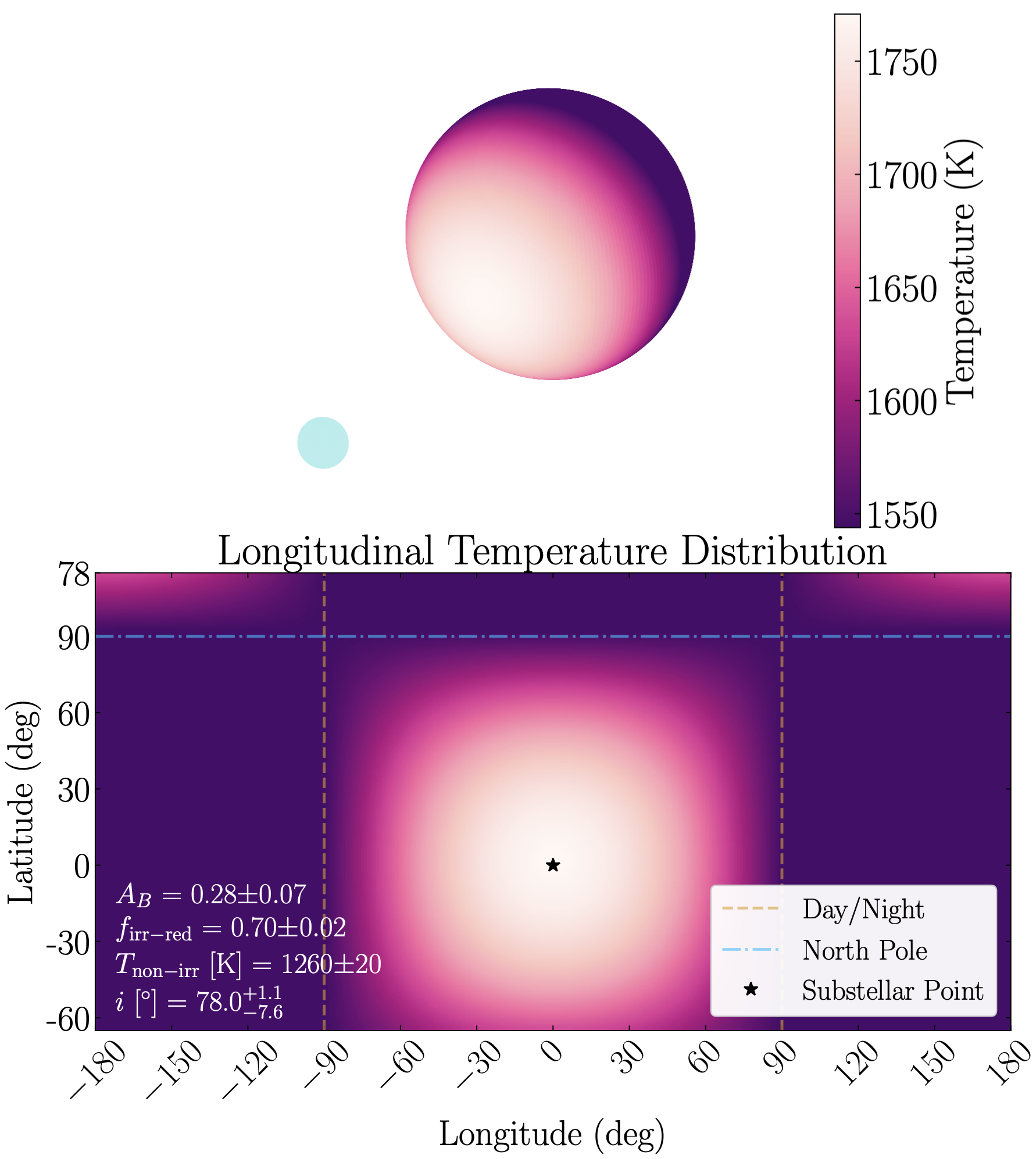
Figure 16: Top: A 3D depiction of the temperature distribution on NLTT5306B. External irradiation comes from the WD primary, represented as a pale blue dot in the lower left. Bottom: A 2D projection of the 3D toy model above with labeled values for Bond albedo, irradiation redistribution fraction, non-irradiated BD temperature, and inclination. The day and night hemisphere-integrated temperatures have a difference of 93 K, matching derived temperature difference in Figure 9.

Table 5: Best Fitting Models

Parameter	Value	Cloudy?	Irradiated?	Parameter	Value	Cloudy?	Irradiated?
Sonora Model Grid				Lothringer et al. Models
Day-side Match		Yes	Yes	Model 1		No	Yes
$T_{\rm{eff}}$ ∗ [K]	1539			$T_{\rm{eff}}$ [K]	1500
$f_{\rm{sed}}$	1.0			log($g$) [cm s-2]	4.50
rfacv	1.0			$[$Fe/H$]$	0.5
Age [Gyr]	3			$f$	0.1
$M_{\rm{BD}}$ [MJup]	70
Night-side Match		Yes	Yes	Model 2		No	Yes
$T_{\rm{eff}}$ [K]	1539			$T_{\rm{eff}}$ [K]	1000
$f_{\rm{sed}}$	3.0			log($g$) [cm s-2]	4.75
rfacv	0.0			$[$Fe/H$]$	0.0
Age [Gyr]	3			$f$	0.5
$M_{\rm{BD}}$ [MJup]	70
Brock et al. Models
Day-side Match		Yes	No	Model 3		Yes	Yes
$T_{\rm{int}}$ [K]	1600			$T_{\rm{eff}}$ [K]	1550
log($g$) [cm s-2]	5.50			log($g$) [cm s-2]	5.50
$[$Fe/H$]$	0.0			$[$Fe/H$]$	0.0
$P_{\rm{c}}$ [bar]	1			$P_{\rm{c}}$ [bar]	20
$K_{\rm{ZZ}}$	1.8			$K_{\rm{ZZ}}$	1.4
$a_{\rm{0}}$ [$\mu$m]	1.0			$a_{\rm{0}}$ [$\mu$m]	0.3
Night-side Match		Yes	No	Model 4		Yes	No
$T_{\rm{int}}$ [K]	1544			$T_{\rm{int}}$ [K]	1544
log($g$) [cm s-2]	5.34			log($g$) [cm s-2]	5.34
$[$Fe/H$]$	0.0			$[$Fe/H$]$	0.0
$P_{\rm{c}}$ [bar]	20			$P_{\rm{c}}$ [bar]	20
$K_{\rm{ZZ}}$	1.4			$K_{\rm{ZZ}}$	1.4
$a_{\rm{0}}$ [$\mu$m]	0.3			$a_{\rm{0}}$ [$\mu$m]	0.3

Note. — ^∗Calculation for $T_{\rm{eff}}$ of the brown dwarf is described in Section 9.1. When there is no external irradiation, $T_{\rm{int}}$ is the only temperature considered.

11.3 Comparing Day/Night Spectra
to field Brown Dwarfs

A comparison of NLTT5306B to field brown dwarfs offers an opportunity to test the extent that external irradiation affects emission spectra of irradiated brown dwarfs. Observed brightness variations in field brown dwarfs are mainly driven by heterogeneous clouds in their atmospheres (e.g., Apai et al., 2013; Buenzli et al., 2014; Metchev et al., 2015; Lew et al., 2020). However, in highly irradiated atmospheres like NLTT5306B, variations can be driven by the phase-dependent irradiation and atmospheric circulation. If the day-to-night energy transport is significant on NLTT5306B, this should introduce excess flux into the night-side spectrum.

To test this hypothesis, we searched the Cloud Atlas spectral library of LTY dwarfs (Manjavacas et al., 2019) for a nearest match using multiple match methods (Section 7.1). Both day and night spectral features of NLTT5306B were best matched with the features of a L4.5 brown dwarf, 2MASS J2224438-015852 (Dupuy & Liu, 2012; Yang et al., 2016), with the night-side being a better fit than the day-side. Silicate clouds are expected to form from condensation in the atmospheres of L dwarfs, but heavy external irradiation might evaporate them. However, with the night-side of NLTT5306B being well-matched with a field brown dwarf spectrum, we conclude that at least within the pressure range probed by our HST observations, the night-side of NLTT5306B and the L4.5 both have hemispherically similar thermal and chemical structures.

The key features of field L dwarf spectra, like deep water absorption around 14,000 Å, are present in both day and night spectra of NLTT5306B. The main deviations between the day-side and the field brown dwarfs occurs at wavelengths less than 12,000 Å. Depending on the structure of NLTT5306B’s atmosphere, this could be due to the fact that these shorter wavelengths are probing different pressure regions (altitudes) or it may be an effect of irradiation, which we further explore through atmospheric modeling.

11.4 1D Brown Dwarf Atmosphere Models

To understand the difference between the day- and night-sides of NLTT5306B and identify spectral signatures of irradiation, we created a variety of one-dimensional atmospheric models for both hemispheres. We considered combinations of cloudy vs. cloud-free and non-irradiated vs. irradiated models from three sources: (1) a grid of PHOENIX models (Section 9.1), (2) a grid of PHOENIX models with opacities from Brock et al. (2021) (Section 8.1), and (3) a grid of SONORA models (Section 9.2). The best-fit models from each source are listed in Table 5.

From all model grids, the night-side spectrum was best matched by atmospheric models that were cloudy and non-irradiated. Given the published system age of at least 5 Gyr, brown dwarf mass of 0.05 M_⊙, one would expect the internal temperature of a field brown dwarf with the same parameters to be less than 1000 K (based on evolutionary models in Burrows et al., 2001). Yet, the night-side of NLTT5306B was best matched by models with internal temperatures between 1500 and 1600 K, suggesting either that NLTT5306B’s cooling and evolution was affected by the external irradiation from the white dwarf primary or that the age estimate is too high. We discuss the possible evolutionary scenarios in Section 11.7.

In fitting 1D models to the day-side of NLTT5306B, models that included clouds and irradiation were a better fit. A model from the Sonora model grid (Figure 13) provided the closest match to the extracted spectrum, with a smaller $f_{\rm{sed}}$ and higher rfacv than the night-side model. However, no fully satisfactory model fits could be found to match spectral features at all wavelengths simultaneously, such as the contrast between the flux at 1.3 $\mu$m and the water absorption at 1.4 $\mu$m and the slopes of the spectrum in the $J$- and $H^{\prime}$-bands.

Given that NLTT5306B is tidally-locked in a tight orbit around a WD primary, it was perhaps not surprising that the day-side spectrum best matched with an irradiated model. This was not necessarily in contrast to the atmospheric parameters found in Section 11.2. Even with a strong $f_{\rm{irr-red}}$ = 0.70$\pm$0.02, the ratio of irradiated flux to internal heat flux for NLTT5306B is small with respect to other WD+BD systems (see Section 11.6). This relatively strong internal heat flux would then still dominate on the night side, whereas the day side is constantly being irradiated, leading to irradiated models being better fits.

11.5 Comparison to Hot Jupiters

Irradiated brown dwarfs differ from field brown dwarfs in that they experience significant external irradiation from a host star, transforming them into excellent analogs to hot Jupiters. One of the key mechanisms believed to impact hot Jupiter atmospheres is the formation/disruption of clouds, which strongly affect atmospheric opacities and pressure-temperature profiles (Burrows et al., 1997; Marley et al., 1999; Ackerman & Marley, 2001; Burrows et al., 2001; Lee et al., 2016; Heng & Demory, 2013). Observations of irradiated brown dwarfs gives us ideal templates when searching for patterns between hot Jupiter properties and their cloud properties.

NLTT5306B orbits its primary star on a much closer orbit than most hot Jupiters. However, the relatively small size of NLTT5306A means the emitting surface area is also small, resulting in an equilibrium temperature of NLTT5306B on the cooler end of temperatures encompassed by hot and ultra-hot Jupiters (e.g. from $\sim 500-5000$ K). For hot Jupiters, the size and intensity of equatorial jets are believed to scale with day-side irradiation (Showman & Guillot, 2002; Showman et al., 2020). In the cloudless GCM of NLTT5306B, a thin jet is present at the equator, with retrograde jets at adjacent latitudes due to the fast rotation (Figure 15). A more detailed GCM is needed to confirm the characteristics of the equatorial jet in this system, but other simulations of irradiated brown dwarfs (Tan & Showman, 2020; Lee et al., 2020) suggest that the rapid rotational timescale (few hours) in WD+BD binaries causes the narrow equatorial jet.

The bottom panel of Figure 17 shows a comparison of Day-Night temperature contrast to external irradiation flux for NLTT5306B, three other WD+BD systems, and hot Jupiters from Komacek & Showman (2016). The hot Jupiters included are HD 189733b (Knutson et al., 2009, 2012), HD 209458b (Crossfield et al., 2012; Zellem et al., 2014), HD 149026b (Knutson et al., 2009), WASP-14b (Wong et al., 2015), WASP-19b (Wong et al., 2016), HAT-P-7b (Wong et al., 2016), and WASP-12b (Cowan et al., 2012). We also include additional hot Jupiters from Beatty et al. (2019) that are not present in the Komacek & Showman (2016) sample. These hot Jupiters are WASP-18b (Maxted et al., 2013), WASP-33b (Zhang et al., 2018; Chakrabarty & Sengupta, 2019), WASP-43b (Stevenson et al., 2017), WASP-103b (Kreidberg et al., 2018). A direct relationship between temperature contrast and external irradiation flux can be seen for both the WD+BD systems and the hot Jupiters. This trend was predicted for hot Jupiters by Showman & Guillot (2002), further supporting the assumption that irradiated brown dwarfs are excellent analogs for hot Jupiters.

One of the few hot Jupiters with a measured spectroscopic phase curve is WASP-43b (Stevenson et al., 2014), which has an equilibrium temperature around 1426 K (Esposito et al., 2017) and a primary host star of spectral type K7 (Salz et al., 2015). From the spectroscopic phase curve of WASP-43b, Stevenson et al. (2014) observed wavelength-dependent phase offsets, much like what is seen in NLTT5306B. In WASP-43b, there was a visible correlation between the day-side thermal emission contribution levels and phase-curve peak offsets as a function of wavelength (see Figure S7 in Stevenson et al., 2014). This is not seen in NLTT5306B when using the best-fit models, but is likely due to our probed pressures not changing by much across our observed HST wavelengths.

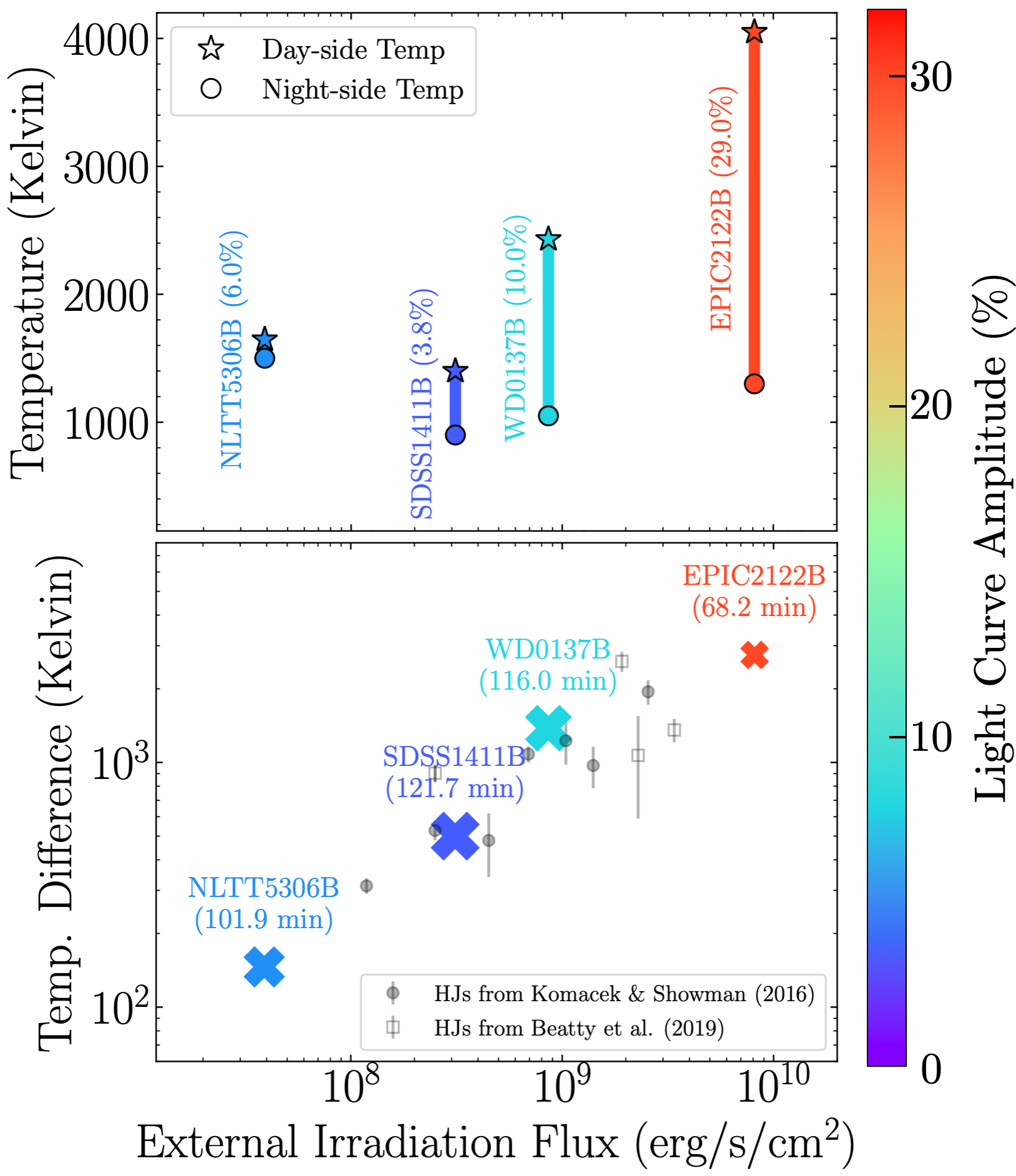
Figure 17: Top: Temperature ranges of NLTT5306B, SDSS1411B, WD0137B, and EPIC2122B versus external irradiation flux from their respective primary white dwarfs. Day- (star) and night-side (circle) hemisphere-averaged brightness temperatures are shown (NLTT5306B has been corrected for inclination). Color represents amplitude of broadband light curves, also labeled next to each name. NLTT5306B does not appear to follow the trend set by the other three systems, where we would expect NLTT5306B to be colder with a smaller light curve amplitude than SDSS1411B. Bottom: Day-Night temperature difference compared to external irradiation flux. Hot Jupiters from Komacek & Showman (2016) and (Beatty et al., 2019). Sizes of WD+BD markers are scaled according to system period, also labeled under each name. A direct relationship between Day-Night difference and irradiation can be seen here despite NLTT5306B’s deviation in the panel above, but there is no obvious relation with system period.

11.6 Comparison to WD 0137B,
EPIC 2122B, and SDSS1411-B

NLTT5306B is the fourth irradiated brown dwarf to be studied in the “Dancing with the Dwarfs” data set, obtained under the HST program GO-15947 (PI: Apai). WD 0137B, EPIC 2122B (Zhou et al., 2022), and SDSS1411-B (Lew et al., 2022) are the previous three that have already been analyzed and published. Analysis of additional data sets in this program are ongoing, but here we present a preliminary comparison with these four WD+BD systems (Figure 17).

WD 0137B, EPIC 2122B, and SDSS1411-B all receive higher levels of irradiation from their primary white dwarfs than NLTT5306B (approximately 22, 208, and 8 times higher, respectively). They also exhibit differing light curve amplitudes (i.e., day/night-side intensity differences) of 10, 29, and 3.8%, respectively (Zhou et al., 2022; Lew et al., 2022). In the top panel of Figure 17, following the relationship established by the other three WD+BD systems, we would expect NLTT5306B to have cooler brightness temperatures and a smaller light curve amplitude than SDSS1411-B. Yet, NLTT5306B deviated from this expectation, which we attribute to the high internal heat flux.

Conversely, in the bottom panel of Figure 17, NLTT5306B appeared to follow a direct relationship between external irradiation and day/night temperature contrast. Note that the temperature difference here was corrected for the effect of inclination (see Section 11.2). After applying a $10\%$ flux increase (decrease) to the day (night) BD spectra and re-deriving brightness temperatures, the temperature difference increased from $93\pm 32$ K (Figure 9) to $146\pm 33$ K. Another important factor in day/night temperature contrast is the rotation rate of the BD (Tan & Showman, 2020), which is inversely proportional to the orbital period in tidally locked companions. Yet NLTT5306B has the second shortest period, and thus second highest rotation rate, in this sample. Tan & Showman (2020) predicted that day/night temperature contrasts would increase with increasing rotation rate, however NLTT5306B deviates from this expectation, another consequence of the strong internal heat flux. So far, it is clear that this growing sample of WD+BD pairs is diverse in many aspects, including irradiation strength, rotation rate, and day/night temperature contrast.

Additionally, in the wavelengths observed by HST, the day- and night-sides of WD 0137B, EPIC 2122B, and SDSS1411-B show significantly different spectral features due to irradiation (see Figure 8 in Zhou et al. (2022) and Figure 9 in Lew et al. (2022)), whereas NLTT5306B displays very similar features between both hemispheres. This is not unexpected, as NLTT5306B receives much weaker irradiation than the other WD+BD systems. This may indicate that higher irradiation induces greater contrasts, but other factors – such as heat redistribution efficiency and opacities – also affect this relationship.

A key difference between NLTT5306B and the other three WD+BD systems is the presence of wavelength-dependent phase offsets. The complex nature of the relative phase offsets seen in Figures 22 and 23 were not present in the phase curves WD 0137B, EPIC 2122B, or SDSS1411-B. More advanced, self-consistent 3D modeling across all systems in this program will be required to confidently identify the source of this difference.

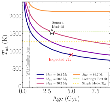
Figure 18: Evolution tracks of four brown dwarf masses according to Sonora Bobcat 2018 tables. A gray dot-dashed line depicts the published WD cooling age from Steele et al. (2013). A red X marks the predicted temperature for a $M_{\rm{BD}}\sim 50$ M_J brown dwarf at 5 Gyr. Observations and models of NLTT5306B do not fit to this prediction. The best-fit night-side $T_{\rm{int}}$ from the Lothringer model grid is shown as a green dashed line. Predicted $T_{\rm{int}}$ from the simple model grid is shown as a golden dotted line. The best night-side match from the Sonora model grid was a $M_{\rm{BD}}=70.2$ M_J at 3 Gyr.

11.7 Evolution of NLTT5306B

Brown dwarfs cool as they age, with more massive brown dwarfs cooling at a slower rate than their less massive counterparts. This is illustrated in Figure 18, where the cooling curves for four brown dwarf masses from the Sonora Bobcat 2018 tables (Marley et al., 2018) are shown. Steele et al. (2013) estimated the system age of NLTT5306 to be at least 5 Gyr, based on the systemic WD velocity, particularly the $U$ component (Johnson & Soderblom, 1987), which generally placed NLTT3506 within the thick-disc population (see Figure 4 of Pauli et al. (2006)). Based on Figure 18, if NLTT5306B were a 5 Gyr, 56$\pm$3 M_Jup field brown dwarf, one would expect the interior heat to be less than 1000 K (presented as a red X). However, our derived brightness temperatures and simple model grid results suggested that NLTT5306B has internal temperature around 1200$-$1300 K.

It is clear that the $T_{\rm{int}}$ evolution of NLTT5306B does not fit to what is expected for a $\sim$50 M_Jup field brown dwarf at 5 Gyr, suggesting either that (1) interaction with the white dwarf primary has affected the evolutionary cooling of the brown dwarf or (2) the system is actually younger than 5 Gyr. Two explanations for scenario (1) could include a reduced internal cooling rate (e.g., Burrows et al., 2007; Chabrier et al., 2007; Chabrier & Baraffe, 2007; Fortney et al., 2021), a deep internal deposition of heat from the primary star (Guillot & Showman, 2002; Batygin & Stevenson, 2010; Sainsbury-Martinez et al., 2021). However, the high internal heat flux in NLTT5306B suggests that the cooling rate has not been sufficiently reduced at the moment. Furthermore, even if 100% of the stellar irradiation was deposited into the interior of the BD, it would still be a small fraction of the observed internal flux, meaning that both mechanisms for scenario (1) are unlikely.

Scenario (2) is consistent with the high night-side temperature. Previously, Steele et al. (2013) estimated the systemic velocities for NLTT5306 using a distance of $D$=71$\pm$4 pc, equatorial coordinates and parallaxes, and radial velocities from their XSHOOTER and Hobby-Eberly Telescope (HET) data. Focusing on the $U$ value, $U\approx 70$ km s^-1, they concluded that NLTT5306A was most likely a thick-disc object, based on Figure 4 from Pauli et al. (2006). With updated, higher precision parameters from Gaia DR3 (Gaia Collaboration et al., 2016), kinematics for NLTT5306 and over 3,000 other white dwarfs were calculated by Raddi et al. (2022).

To determine the new age of NLTT5306B, we downloaded Tables 4 and 7 from Raddi et al. (2022) and extracted the ages of thin-disc only systems, i.e. only systems with $e<$ 0.27. We then calculated two total ages for every system by summing the WD cooling age with the two progenitor age estimates from the Catalán et al. (2008) (C08) and Cummings et al. (2018) (C18) initial-to-final-mass relations. Since NLTT3506A has a cooling age of 710 Myr, we ignored ages younger than 0.7 Gyr, resulting in age peaks around 1 Gyr for C08 and 2 Gyr for C18. Therefore, we approximate the system age of NLTT5306B to most likely be 1-2 Gyr, which essentially removed the age vs. internal temperature discrepancy for NLTT5306B and reaffirmed our conclusion that this BD is dominated by internal heat flux.

12 Conclusions

In this study, we presented time-resolved, high-precision spectrophotometric, rotational phase mapping of the irradiated brown dwarf NLTT5306. The key findings of our study are as follows:

• We presented high-quality HST/WFC3/G141 phase-resolved spectra of white dwarf-brown dwarf binary NLTT5306. The observations sampled approximately 90% of the rotational phase of this system and exhibited moderate photometric and spectroscopic variations.

• We modeled the light curve of NLTT5306 to within 0.5%. The period of the favored 1st-order phase curve model created in this work (102.05$\pm$0.07 min) is longer than the published period of 101.88$\pm$0.02 min (Steele et al., 2013).

• The synthetic light curves made in the $J$-, Water Absorption, and $H^{\prime}$-bands had peak-to-trough amplitudes between $\sim$5-7% and relative phase offsets up to 6.8$\pm$0.3^∘.

• Synthetic light curves made from narrower wavelength bins (Section A) exhibited a prominent wavelength dependence on amplitudes and phase offsets. This indicated a complex longitudinal-vertical atmospheric structure.

• After modeling and subtracting the white dwarf contribution, we extracted phase-resolved brown dwarf spectra, with a day-side approximately 40% brighter than the night-side. Both the day and night spectra were well fit by an L4.5 spectral type field brown dwarf spectrum from the Cloud Atlas catalog.

• Although the day and night brightness temperatures of NLTT5306B were highly wavelength dependent, the temperature difference was nearly constant at 93 K (or 5% of the average day side temperature). This suggested efficient day/night heat redistribution.

• A simple radiative and energy redistribution model reproduced well both the observed day- and night-side temperatures. The model suggested an $A_{B}$ = 0.28$\pm$0.07, $f_{\rm{irr-red}}$ = 0.70$\pm$0.02, $T_{\rm{non-irr}}$ = 1260$\pm$20 K, and $i$ = $78.0^{+1.1}_{-7.6}$ degrees for NLTT5306B.

• The day-side of NLTT5306B was well but not perfectly fit with an irradiated, cloudy 1D model. The night-side was fit by a non-irradiated, cloudy model.

• A general circulation model is presented that explains the observed, relatively small day-to-night-side temperature difference. The small difference is due to the relatively weak irradiation (with respect to the internal heat flux).

• The internal temperatures predicted for NLTT5306B by Sonora Bobcat 2018 and Lothringer models were inconsistent with the age previously reported (Steele et al., 2013). Our reassessment of the age estimate suggested NLTT5306A to be much younger ($\sim$1$-$2 Gyr), which was fully consistent with the evolutionary model predictions.

• The range of likely inclinations for NLTT5306 were constrained to $i=78.0^{+1.1}_{-7.6}$ degrees, yielding a flux correction factor of $+10\%$ for the day-side and $-10\%$ for the night-side. We explored the impact this uncertainty would have on the results of simple atmosphere model, and found that only one parameter, Bond albedo, was sensitive to the unknown inclination.

Our comprehensive analysis shows that the brown dwarf in the NLTT5306 system is one of the least irradiated brown dwarfs known to be in a tidally-locked orbit, bridging the gap between highly irradiated brown dwarfs and field brown dwarfs. Given the re-assessed age, this is also a relatively young system where the internal heat still outcompetes the irradiation from its white dwarf host.

Appendix A Wavelength-Dependent Phase Offsets and Modulation Amplitudes

Motivated by the $>$5 degree phase offsets and $>$1% amplitude differences between the $H^{\prime}$-band and the other synthetic light curves, we performed a more detailed analysis to pinpoint which wavelengths contributed most to the observed behavior. By narrowing down the wavelengths, we can also point to the chemical species that is the dominant absorber in that wavelength range, helping us a paint a clearer picture of the atmospheric dynamics at play.

We split the spectra into 40 wavelength bins that are each 137 Å wide, allowing for some overlap between the new bins, as shown in Figure 19. When creating the new light curves, filter response functions were not applied, i.e. 2MASS $J$ and $H^{\prime}$ used previously for the synthetic light curves. Our intention was to ensure that the differences between bins were real and not the result of being exaggerated by the tail ends of response functions. The 40 new light curves are presented in Figures 20 and 21, along with their 1st and 2nd order phase curves models, respectively.

Similar to the phase curve fitting functions described before, we used an MCMC to find the best-fit phase curve for both a 1st and 2nd order sinusoidal function. The residuals produced by subtracting each model from the data didn’t show much preference for either order, so we included both for comparison. For each light curve, we produced 10,000 phase curve models with a burn of 1,000, leaving 9,000 models to find the best-fit phase curve parameters. The resulting median and 1-sigma uncertainties for phase offsets and modulation amplitudes are shown in Figures 22 and 23. Phase offsets are calculated with respect to the peak of the $J$-band phase curve model.

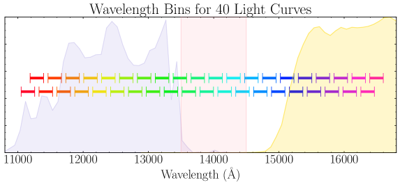
Figure 19: Locations of new wavelength bins used to investigate the wavelength dependence of phase offsets and amplitudes. The old light curve filters, 2MASS $J$- (purple), Water (pink), and 2MASS $H$-band (yellow), are shown as a reference, but are not applied to the new light curves. For easier viewing, the new wavelength bins have been staggered on top of each other. Each new bin spans 137 Å with $\sim$2/3 of each bin overlapping with its neighboring bins.

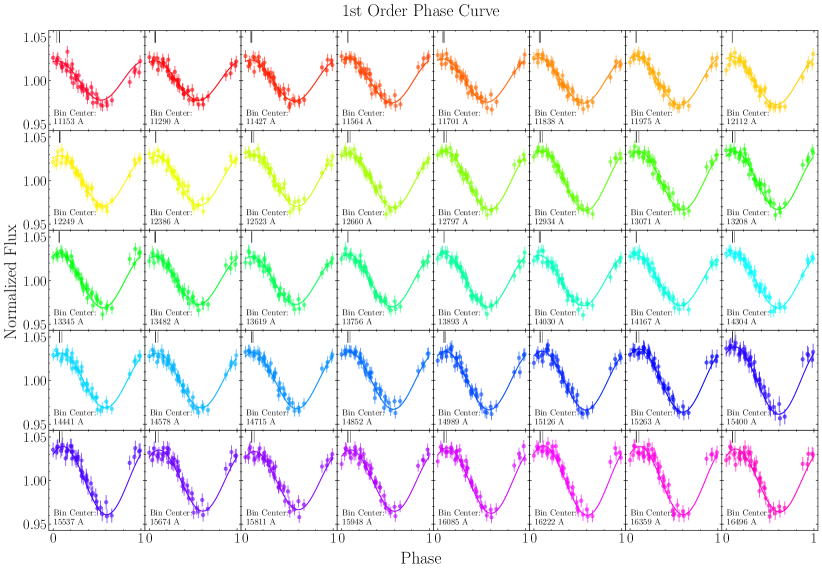
Figure 20: Period-folded phase curves created from 40 narrow (136 Å) wavelength bins and assuming a 1st-Order phase curve model. The wavelength of the bin centers are noted in the bottom left of each plot. Phase offsets for these phase curves are calculated from the difference between the peaks of these models (gray vertical line) and the $J$-band peak (black vertical line). So, the farther apart the vertical lines appear in phase space, the greater the phase offset.

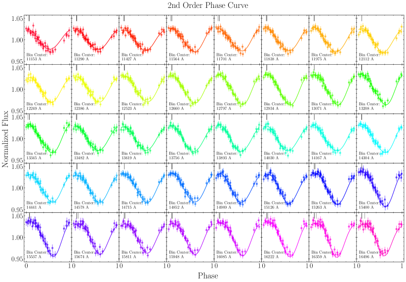
Figure 21: Similar to Figure 20, except these phase curves models are made with a combination of $k$=1,2 sinusoidal functions (see Equation 2).

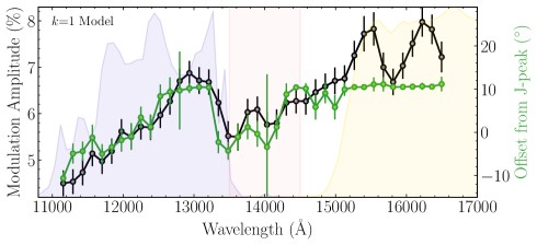
Figure 22: The modulation amplitudes (black) and phase offsets (green) of the 1st-order ($k$=1) phase curves, corresponding to Figure 20. The high SNR of our data allows us to conduct this detailed investigation into the wavelength dependence on amplitude and phase. Although they were not applied here, the old light curve filters (i.e. 2MASS $J$, Water Absorption, and 2MASS $H$) are shown in the background as a reference. Error bars depict 1$\sigma$ uncertainty from the MCMC chains. The phase offset curve seems to generally follow the same shape as the amplitude curve until reaching the $H^{\prime}$-band wavelengths. After 15,000 Å, the phase offsets appear to remain constant, even though the amplitude curve reaches its highest peaks here.

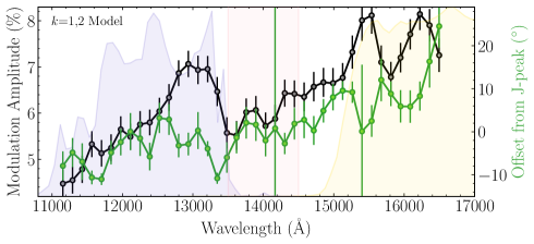
Figure 23: Similar to Figure 22, except these amplitudes and offsets correspond the 2nd order ($k$=1,2) phase curve models in Figure 21. Here, the phase offset curve again seems to follow to the modulation amplitude curve, except for when the amplitude curve peaks above 7% around three wavelengths: 12,900, 15,450 and 16,250 Å. When the modulation amplitude curve begins to peak, the phase offset curve begins to dip. It remains unknown why an anti-correlation would be present.

Appendix B Flux Scaling Cloud Atlas Spectra to Photometry of NLTT5306B

In Table 1 of Manjavacas et al. (2019), the authors report a 2MASS $J$-band magnitude for each L, T, Y dwarf. We use this magnitude to photometrically scale the spectra to the expected $J$-band magnitudes of the day- and night-sides of NLTT5306B. We estimated what the day- and night-side magnitudes would be by solving the equation for apparent magnitudes and flux ratios:

$$m_{J,\rm{BD}}=m_{J,\rm{WD+BD}}-2.5~{}\rm{log_{10}}\Big{(}\frac{\overline{F}_{J\rm{,BD}}}{\overline{F}_{J\rm{,WD+BD}}}\Big{)}$$ (B1)

where $m_{J\rm{,BD}}$ is the brown dwarf magnitude we are looking for, $m_{J\rm{,WD+BD}}$ is the $J$-band magnitude of the white dwarf + brown dwarf system ($m_{J\rm{,WD+BD}}$=16.23), $\overline{\rm{F}}_{J\rm{,WD+BD}}$ is the mean flux value in the $J$-band of the observed white dwarf + brown dwarf spectrum, and $\overline{\rm{F}}_{J\rm{,BD}}$ is the average flux in the $J$-band of the extracted brown dwarf spectrum. From this equation, we found that $m_{J}$(BD_Day) = 18.08 $\pm$ 0.22 and $m_{J}$(BD_Night) = 18.40 $\pm$ 0.31. When using the “flux scaling” match method (e.g., top row of Figure 10), the Cloud Atlas spectra were scaled to these magnitudes.

Appendix C Grid Search Among Bond Albedo, Irradiation Redistribution Fraction, Non-Irradiated BD Temperature, and Inclination

We conducted a grid among 4 parameters: (1) Bond albedo, $A_{B}$ = [0.0, 1.0] in increments of 0.025, (2) irradiation redistribution fraction, $f_{\rm{irr-red}}$, sampled between 0.0 and 1.0 in increments of 0.02, (3) non-irradiated brown dwarf temperature, $T_{\rm{non-irr}}$, sampled from 800 to 2000 K in increments of 10 K, and (4) inclination, $i$, from 57 to 85 degrees in increments of 0.5. For each combination of parameters, the first step was to apply a uniform day- and night-side temperature set by the input $T_{\rm{non-irr}}$. Then, incident radiation from the WD was added to the day-side, and the value of $A_{B}$ determined how much was reflected away. In this tidally-locked set-up, the substellar point is the hottest location on the BD surface for all $A_{B}<$1.0. Next, we redistributed a fraction of the incident radiation from the day-side, determined by $f_{\rm{irr-red}}$, and evenly distributed it onto the BD entire surface. If $f_{\rm{irr-red}}$ = 1.0, all irradiated flux would be evenly redistributed, resulting in a uniform temperature map. Finally, we added the effect of inclination by taking a number of rows at the top of the temperature map and switching them between day and night hemispheres. The number of rows were determined by the inclination parameter, where a lower inclination would result in a larger amount of rows, due to the greater percentage of the opposite hemisphere being seen. To determine the best-fit set of parameters, we calculated residuals between each temperature distribution map and our observables, i.e. brightness temperatures.

Since brightness temperatures are a hemisphere-integrated quantity, we calculated the day and night hemisphere-integrated temperatures for each map ($T_{\rm{map,day}}$ and $T_{\rm{map,night}}$), where day is defined as $-$90${}^{\circ}>$longitude$>$90^∘ and night $-$90${}^{\circ}\geq$longitude$\leq$90^∘ (see Figure 16). From our brightness temperatures and 1D modeling results, we assumed the observed night-side temperature to be $T_{\rm{BD,night}}$=1500$\pm$20 K. Then, from Figure 9, we assumed $T_{\rm{BD,day}}$=$T_{\rm{BD,night}}+93$ K=1593$\pm$30 K. The residuals were calculated via the following:

$$R=\left(\frac{T_{\rm{BD,day}}-T_{\rm{map,day}}}{\sigma_{\rm{BD,day}}}\right)^{2}+\left(\frac{T_{\rm{BD,night}}-T_{\rm{map,night}}}{\sigma_{\rm{BD,night}}}\right)^{2}$$ (C1)

We accepted the smallest value of R as the correct answer, and also checked that the combination of parameters was within the realm of realistically physical values. The combination that resulted in the smallest R was $A_{B}$ = 0.28$\pm$0.07, $f_{\rm{irr-red}}$ = 0.70$\pm$0.02, $T_{\rm{non-irr}}$ = 1260$\pm$20 K. and $i=78.0^{+1.1}_{-7.6}$ degrees. While this temperature distribution model is fairly simple and cannot capture more complex dynamics, we believe such an approach is a useful starting point for understanding observations of tidally-locked atmospheres.

Appendix D Effect of Inclination

Exploring the effects of inclination on observational constraints and results provides a more accurate view of systems and their dynamics. To get a better understanding of how unknown inclination impacts our results, we created an exploratory atmosphere model. In this basic model, there are only two hemispheres, day and night, where the night-side temperature is determined by the internal brown dwarf temperature (i.e. non-irradiated temperature) and the day-side is exposed to the same amount of external irradiation as NLTT5306B. In the absence of atmospheric circulation, the irradiation temperature at the substellar point on NLTT5306B is around 910 K. Depending on the internal brown dwarf temperature, 910 K could create a moderate to large flux contrast between the day- and night-sides. We show this effect for range of non-irradiated brown dwarf temperatures from 900 to 1600 K, coupled with the effect of inclination in the left panel of Figure 24.

The fluxes for day and night, F_Day and F_Night, were calculated by creating a basic version of the atmosphere model from Section 11.2 for each non-irradiated BD temperature. This version of the atmosphere model ignores $A_{B}$ and $f_{\rm{irr-red}}$. We then took the hemisphere-integrated temperature for both day- and night-sides and converted them into fluxes via F$\propto$T⁴. We imagined a system orientation where the the brown dwarf is farthest from the observer. Figure 24 shows the total observed flux as a function of inclination, according to the following equations:

$$F(i) =F_{\rm{Day}}(i)+F_{\rm{Night}}(i),$$ (D1)

$$F_{\rm{Day}}(i) =F_{\rm{Day}}(90^{\circ})\Big{(}1-\frac{1}{2}\rm{cos}(i)\Big{)},$$

$$F_{\rm{Night}}(i) =F_{\rm{Night}}(90^{\circ})\Big{(}\frac{1}{2}\rm{cos}(i)\Big{)}.$$

For equatorial viewing geometry ($i=90^{\circ}$), only the day-side would be visible. However, for any other inclinations, a fraction of the night-side hemisphere would be simultaneously visible, causing the observed hemisphere to appear dimmer than it really is (illustrated in the top right panel of Figure 24). In contrast, if we were to observe the night-side hemisphere at inclinations other than 90^∘, the partially visible day-side would cause the hemisphere to appear brighter. Our model accounts for this and helps to assess the importance of this effect.

Based on our exploratory model, we find that the effect of uncertain inclination (within a constrained range) would impact the derived fluxes by 7 to 25% (relative to the equatorial view), as shown in the bottom right panel of Figure 24. Thus, to obtain a more physically accurate view of NLTT5306B’s atmosphere, we included the inclination as a parameter in the simple atmosphere model. Through a grid search, we constrained possible values for the Bond albedo ($A_{B}$), irradiation redistribution fraction ($f_{\rm{irr-red}}$), non-irradiated BD temperature ($T_{\rm{non-irr}}$), and inclination ($i$). Inclination was constrained to $78.0^{+1.1}_{-7.6}$ degrees (see 11.2). At $78.0^{\circ}$ inclination, our observed day- and night-side flux values would need to be corrected by $+10\%$ (for day-side) and $-10\%$ (for night-side) in order to get the likely true flux for each hemisphere.

Next, after we ran the grid model search with all 4 parameters (see Section 11.2), we determined how correlated the inclination is with the other parameters. We searched for correlation by using the four-dimensional grid of chi-squared values, collapsed down to the 2 axes of interest. The result of this method is shown in Figure 25. We used dashed lines to indicate the likely range of inclinations. We find little to no correlation between $i$ inclination and the following two parameters: irradiation redistribution fraction ($f_{\rm{irr-red}}$) and non-irradiated BD temperature ($T_{\rm{non-irr}}$). Therefore, the derived irradiation redistribution fraction and non-irradiated BD temperature are insensitive to the uncertainty in the inclination and are thus robust values. However, the derived Bond albedo is somewhat sensitive to the exact inclination, with the $A_{B}$ varying between 0.15 to 0.47 for likely inclination range of $78.0^{+1.1}_{-7.6}$.

Figure 24: Left: The effect of inclination on derived flux seen at an orientation where the day-side dominates, .i.e, the brown dwarf is farthest from the observer. Inclinations other than $i=90^{\circ}$ result in the night-side being partially visible, which decreases the derived flux. The green shaded region shows the possible inclinations for NLTT5306. Top Right: Flux contributions from the day and night hemispheres as a function of inclination. As we increase inclination, we see more of the day side and less of the night side. Bottom Right: Flux correction factors for each non-irradiated brown dwarf temperature considered in the left panel, determined by the expression in the upper right corner. Both the low ($i=58^{\circ}$) and high ($i=79.7^{\circ}$) ends of the possible inclination range for NLTT5306 are shown as diamonds and stars, respectively. From this panel, we conclude that the flux correction factor for NLTT5306B could be between 7 and 25%.

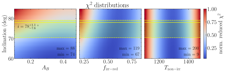
Figure 25: Distribution of normalized chi-squared values from the atmospheric model grid search conducted in Section 11.2. Minimum and maximum values used to normalize each distribution are labeled in the bottom right of each panel. Panels show relationships between inclination and the other three parameters: Bond albedo ($A_{B}$), fraction of irradiation redistributed from day-to-night ($f_{\rm{irr-red}}$), and non-irradiated BD temperature ($T_{\rm{non-irr}}$). Lower values of chi-squared indicate better fits to the observations. Best-fit inclination for NLTT5306B is shown as a solid yellow line, with 1-sigma uncertainty shown as dashed yellow lines. In the middle and right panels, there is little to no correlation between these parameters and inclination. However, the left-most panel shows that Bond albedo, $A_{B}$, is mildly sensitive to the inclination.

References

- Ackerman & Marley (2001) Ackerman, A. S., & Marley, M. S. 2001, ApJ, 556, 872, doi: 10.1086/321540
- Allard et al. (2001) Allard, F., Hauschildt, P. H., Alexander, D. R., Tamanai, A., & Schweitzer, A. 2001, ApJ, 556, 357, doi: 10.1086/321547
- Apai et al. (2013) Apai, D., Radigan, J., Buenzli, E., et al. 2013, ApJ, 768, 121, doi: 10.1088/0004-637X/768/2/121
- Arcangeli et al. (2021) Arcangeli, J., Désert, J. M., Parmentier, V., Tsai, S. M., & Stevenson, K. B. 2021, A&A, 646, A94, doi: 10.1051/0004-6361/202038865
- Arcangeli et al. (2018) Arcangeli, J., Désert, J.-M., Line, M. R., et al. 2018, ApJ, 855, L30, doi: 10.3847/2041-8213/aab272
- Arcangeli et al. (2019) Arcangeli, J., Désert, J.-M., Parmentier, V., et al. 2019, A&A, 625, A136, doi: 10.1051/0004-6361/201834891
- Astropy Collaboration et al. (2013) Astropy Collaboration, Robitaille, T. P., Tollerud, E. J., et al. 2013, A&A, 558, A33, doi: 10.1051/0004-6361/201322068
- Astropy Collaboration et al. (2018) Astropy Collaboration, Price-Whelan, A. M., Sipőcz, B. M., et al. 2018, AJ, 156, 123, doi: 10.3847/1538-3881/aabc4f
- Barber et al. (2006) Barber, R. J., Tennyson, J., Harris, G. J., & Tolchenov, R. N. 2006, MNRAS, 368, 1087, doi: 10.1111/j.1365-2966.2006.10184.x
- Batalha et al. (2019) Batalha, N. E., Marley, M. S., Lewis, N. K., & Fortney, J. J. 2019, ApJ, 878, 70, doi: 10.3847/1538-4357/ab1b51
- Batygin & Stevenson (2010) Batygin, K., & Stevenson, D. J. 2010, ApJ, 714, L238, doi: 10.1088/2041-8205/714/2/L238
- Beatty et al. (2019) Beatty, T. G., Marley, M. S., Gaudi, B. S., et al. 2019, AJ, 158, 166, doi: 10.3847/1538-3881/ab33fc
- Bertin & Arnouts (1996) Bertin, E., & Arnouts, S. 1996, A&AS, 117, 393, doi: 10.1051/aas:1996164
- Beuermann et al. (2013) Beuermann, K., Dreizler, S., Hessman, F. V., et al. 2013, A&A, 558, A96, doi: 10.1051/0004-6361/201322241
- Brock et al. (2021) Brock, L., Barman, T., Konopacky, Q. M., & Stone, J. M. 2021, ApJ, 914, 124, doi: 10.3847/1538-4357/abfc46
- Buenzli et al. (2014) Buenzli, E., Apai, D., Radigan, J., Reid, I. N., & Flateau, D. 2014, ApJ, 782, 77, doi: 10.1088/0004-637X/782/2/77
- Buenzli et al. (2012) Buenzli, E., Apai, D., Morley, C. V., et al. 2012, ApJ, 760, L31, doi: 10.1088/2041-8205/760/2/L31
- Burrows et al. (2001) Burrows, A., Hubbard, W. B., Lunine, J. I., & Liebert, J. 2001, Reviews of Modern Physics, 73, 719, doi: 10.1103/RevModPhys.73.719
- Burrows et al. (2007) Burrows, A., Hubeny, I., Budaj, J., & Hubbard, W. B. 2007, ApJ, 661, 502, doi: 10.1086/514326
- Burrows et al. (1997) Burrows, A., Marley, M., Hubbard, W. B., et al. 1997, ApJ, 491, 856, doi: 10.1086/305002
- Buzard et al. (2022) Buzard, C., Casewell, S., Lothringer, J., & Blake, G. 2022, arXiv e-prints, arXiv:2204.05330. https://arxiv.org/abs/2204.05330
- Carnall (2017) Carnall, A. C. 2017, arXiv e-prints, arXiv:1705.05165. https://arxiv.org/abs/1705.05165
- Casewell et al. (2020a) Casewell, S. L., Debes, J., Braker, I. P., et al. 2020a, MNRAS, 499, 5318, doi: 10.1093/mnras/staa3184
- Casewell et al. (2012) Casewell, S. L., Burleigh, M. R., Wynn, G. A., et al. 2012, ApJ, 759, L34, doi: 10.1088/2041-8205/759/2/L34
- Casewell et al. (2018) Casewell, S. L., Braker, I. P., Parsons, S. G., et al. 2018, MNRAS, 476, 1405, doi: 10.1093/mnras/sty245
- Casewell et al. (2020b) Casewell, S. L., Belardi, C., Parsons, S. G., et al. 2020b, MNRAS, 497, 3571, doi: 10.1093/mnras/staa1608
- Catalán et al. (2008) Catalán, S., Isern, J., García-Berro, E., & Ribas, I. 2008, MNRAS, 387, 1693, doi: 10.1111/j.1365-2966.2008.13356.x
- Chabrier & Baraffe (2007) Chabrier, G., & Baraffe, I. 2007, ApJ, 661, L81, doi: 10.1086/518473
- Chabrier et al. (2007) Chabrier, G., Gallardo, J., & Baraffe, I. 2007, A&A, 472, L17, doi: 10.1051/0004-6361:20077702
- Chakrabarty & Sengupta (2019) Chakrabarty, A., & Sengupta, S. 2019, AJ, 158, 39, doi: 10.3847/1538-3881/ab24dd
- Cowan et al. (2012) Cowan, N. B., Machalek, P., Croll, B., et al. 2012, ApJ, 747, 82, doi: 10.1088/0004-637X/747/1/82
- Cranmer (2021) Cranmer, S. R. 2021, Research Notes of the American Astronomical Society, 5, 201, doi: 10.3847/2515-5172/ac225c
- Crossfield et al. (2012) Crossfield, I. J. M., Knutson, H., Fortney, J., et al. 2012, ApJ, 752, 81, doi: 10.1088/0004-637X/752/2/81
- Cummings et al. (2018) Cummings, J. D., Kalirai, J. S., Tremblay, P. E., Ramirez-Ruiz, E., & Choi, J. 2018, ApJ, 866, 21, doi: 10.3847/1538-4357/aadfd6
- Cushing et al. (2006) Cushing, M. C., Roellig, T. L., Marley, M. S., et al. 2006, ApJ, 648, 614, doi: 10.1086/505637
- Dupuy & Liu (2012) Dupuy, T. J., & Liu, M. C. 2012, ApJS, 201, 19, doi: 10.1088/0067-0049/201/2/19
- Eastman et al. (2010) Eastman, J., Siverd, R., & Gaudi, B. S. 2010, PASP, 122, 935, doi: 10.1086/655938
- Esposito et al. (2017) Esposito, M., Covino, E., Desidera, S., et al. 2017, A&A, 601, A53, doi: 10.1051/0004-6361/201629720
- Foreman-Mackey et al. (2013) Foreman-Mackey, D., Hogg, D. W., Lang, D., & Goodman, J. 2013, PASP, 125, 306, doi: 10.1086/670067
- Fortney et al. (2021) Fortney, J. J., Dawson, R. I., & Komacek, T. D. 2021, Journal of Geophysical Research (Planets), 126, e06629, doi: 10.1029/2020JE006629
- Gaia Collaboration et al. (2016) Gaia Collaboration, Prusti, T., de Bruijne, J. H. J., et al. 2016, A&A, 595, A1, doi: 10.1051/0004-6361/201629272
- Gao & Powell (2021) Gao, P., & Powell, D. 2021, ApJ, 918, L7, doi: 10.3847/2041-8213/ac139f
- Girven et al. (2011) Girven, J., Gänsicke, B. T., Steeghs, D., & Koester, D. 2011, MNRAS, 417, 1210, doi: 10.1111/j.1365-2966.2011.19337.x
- Guillot & Showman (2002) Guillot, T., & Showman, A. P. 2002, A&A, 385, 156, doi: 10.1051/0004-6361:20011624
- Harre & Heller (2021) Harre, J.-V., & Heller, R. 2021, Astronomische Nachrichten, 342, 578, doi: 10.1002/asna.202113868
- Harris et al. (2020) Harris, C. R., Millman, K. J., van der Walt, S. J., et al. 2020, Nature, 585, 357, doi: 10.1038/s41586-020-2649-2
- Heng & Demory (2013) Heng, K., & Demory, B.-O. 2013, ApJ, 777, 100, doi: 10.1088/0004-637X/777/2/100
- Heng & Showman (2015) Heng, K., & Showman, A. P. 2015, Annual Review of Earth and Planetary Sciences, 43, 509, doi: 10.1146/annurev-earth-060614-105146
- Hunter (2007) Hunter, J. D. 2007, Computing in Science & Engineering, 9, 90, doi: 10.1109/MCSE.2007.55
- Johnson & Soderblom (1987) Johnson, D. R. H., & Soderblom, D. R. 1987, AJ, 93, 864, doi: 10.1086/114370
- Kitzmann et al. (2018) Kitzmann, D., Heng, K., Rimmer, P. B., et al. 2018, ApJ, 863, 183, doi: 10.3847/1538-4357/aace5a
- Knutson et al. (2007) Knutson, H. A., Charbonneau, D., Allen, L. E., et al. 2007, Nature, 447, 183, doi: 10.1038/nature05782
- Knutson et al. (2009) Knutson, H. A., Charbonneau, D., Cowan, N. B., et al. 2009, ApJ, 690, 822, doi: 10.1088/0004-637X/690/1/822
- Knutson et al. (2012) Knutson, H. A., Lewis, N., Fortney, J. J., et al. 2012, ApJ, 754, 22, doi: 10.1088/0004-637X/754/1/22
- Koester (2010) Koester, D. 2010, Mem. Soc. Astron. Italiana, 81, 921
- Komacek & Showman (2016) Komacek, T. D., & Showman, A. P. 2016, ApJ, 821, 16, doi: 10.3847/0004-637X/821/1/16
- Komacek et al. (2022) Komacek, T. D., Tan, X., Gao, P., & Lee, E. K. H. 2022, ApJ, 934, 79, doi: 10.3847/1538-4357/ac7723
- Kreidberg et al. (2018) Kreidberg, L., Line, M. R., Parmentier, V., et al. 2018, AJ, 156, 17, doi: 10.3847/1538-3881/aac3df
- Kümmel et al. (2009) Kümmel, M., Walsh, J. R., Pirzkal, N., Kuntschner, H., & Pasquali, A. 2009, PASP, 121, 59, doi: 10.1086/596715
- Kurucz & Bell (1995) Kurucz, R., & Bell, B. 1995, Atomic Line Data (R.L. Kurucz and B. Bell) Kurucz CD-ROM No. 23. Cambridge, 23
- Lee et al. (2016) Lee, E., Dobbs-Dixon, I., Helling, C., Bognar, K., & Woitke, P. 2016, A&A, 594, A48, doi: 10.1051/0004-6361/201628606
- Lee et al. (2020) Lee, E. K. H., Casewell, S. L., Chubb, K. L., et al. 2020, MNRAS, 496, 4674, doi: 10.1093/mnras/staa1882
- Lee et al. (2022) Lee, E. K. H., Lothringer, J. D., Casewell, S. L., et al. 2022, arXiv e-prints, arXiv:2203.09854. https://arxiv.org/abs/2203.09854
- Lew et al. (2020) Lew, B. W. P., Apai, D., Marley, M., et al. 2020, ApJ, 903, 15, doi: 10.3847/1538-4357/abb81d
- Lew et al. (2022) Lew, B. W. P., Apai, D., Zhou, Y., et al. 2022, AJ, 163, 8, doi: 10.3847/1538-3881/ac3001
- Lian et al. (2022) Lian, Y., Showman, A. P., Tan, X., & Hu, Y. 2022, ApJ, 928, 166, doi: 10.3847/1538-4357/ac5598
- Longstaff et al. (2019) Longstaff, E. S., Casewell, S. L., Wynn, G. A., et al. 2019, MNRAS, 484, 2566, doi: 10.1093/mnras/stz127
- Lothringer et al. (2018) Lothringer, J. D., Barman, T., & Koskinen, T. 2018, ApJ, 866, 27, doi: 10.3847/1538-4357/aadd9e
- Lothringer & Casewell (2020) Lothringer, J. D., & Casewell, S. L. 2020, ApJ, 905, 163, doi: 10.3847/1538-4357/abc5bc
- Manjavacas et al. (2019) Manjavacas, E., Apai, D., Zhou, Y., et al. 2019, AJ, 157, 101, doi: 10.3847/1538-3881/aaf88f
- Marley et al. (2018) Marley, M., Saumon, D., Morley, C., & Fortney, J. 2018, Sonora 2018: Cloud-free, solar composition, solar C/O substellar atmosphere models and spectra, nc_m+0.0_co1.0_v1.0, Zenodo, doi: 10.5281/zenodo.1309035
- Marley et al. (2013) Marley, M. S., Ackerman, A. S., Cuzzi, J. N., & Kitzmann, D. 2013, in Comparative Climatology of Terrestrial Planets, ed. S. J. Mackwell, A. A. Simon-Miller, J. W. Harder, & M. A. Bullock, 367–392, doi: 10.2458/azu_uapress_9780816530595-ch015
- Marley et al. (1999) Marley, M. S., Gelino, C., Stephens, D., Lunine, J. I., & Freedman, R. 1999, ApJ, 513, 879, doi: 10.1086/306881
- Marley & Robinson (2015a) Marley, M. S., & Robinson, T. D. 2015a, ARA&A, 53, 279, doi: 10.1146/annurev-astro-082214-122522
- Marley & Robinson (2015b) —. 2015b, ARA&A, 53, 279, doi: 10.1146/annurev-astro-082214-122522
- Marley et al. (2021) Marley, M. S., Saumon, D., Visscher, C., et al. 2021, ApJ, 920, 85, doi: 10.3847/1538-4357/ac141d
- Martin et al. (2018) Martin, E. C., Fitzgerald, M. P., McLean, I. S., et al. 2018, in Society of Photo-Optical Instrumentation Engineers (SPIE) Conference Series, Vol. 10702, Ground-based and Airborne Instrumentation for Astronomy VII, ed. C. J. Evans, L. Simard, & H. Takami, 107020A, doi: 10.1117/12.2312266
- Maxted et al. (2006) Maxted, P. F. L., Napiwotzki, R., Dobbie, P. D., & Burleigh, M. R. 2006, Nature, 442, 543, doi: 10.1038/nature04987
- Maxted et al. (2013) Maxted, P. F. L., Anderson, D. R., Doyle, A. P., et al. 2013, MNRAS, 428, 2645, doi: 10.1093/mnras/sts231
- Mayorga et al. (2019) Mayorga, L. C., Batalha, N. E., Lewis, N. K., & Marley, M. S. 2019, AJ, 158, 66, doi: 10.3847/1538-3881/ab29fa
- McKay et al. (1989) McKay, C. P., Pollack, J. B., & Courtin, R. 1989, Icarus, 80, 23, doi: 10.1016/0019-1035(89)90160-7
- McLean et al. (1998) McLean, I. S., Becklin, E. E., Bendiksen, O., et al. 1998, in Society of Photo-Optical Instrumentation Engineers (SPIE) Conference Series, Vol. 3354, Infrared Astronomical Instrumentation, ed. A. M. Fowler, 566–578, doi: 10.1117/12.317283
- Metchev et al. (2015) Metchev, S. A., Heinze, A., Apai, D., et al. 2015, ApJ, 799, 154, doi: 10.1088/0004-637X/799/2/154
- Mikal-Evans et al. (2023) Mikal-Evans, T., Sing, D. K., Dong, J., et al. 2023, arXiv e-prints, arXiv:2301.03209. https://arxiv.org/abs/2301.03209
- Morley et al. (2012) Morley, C. V., Fortney, J. J., Marley, M. S., et al. 2012, ApJ, 756, 172, doi: 10.1088/0004-637X/756/2/172
- Parmentier et al. (2021) Parmentier, V., Showman, A. P., & Fortney, J. J. 2021, MNRAS, 501, 78, doi: 10.1093/mnras/staa3418
- Parmentier et al. (2018) Parmentier, V., Line, M. R., Bean, J. L., et al. 2018, A&A, 617, A110, doi: 10.1051/0004-6361/201833059
- Parsons et al. (2017) Parsons, S. G., Hermes, J. J., Marsh, T. R., et al. 2017, MNRAS, 471, 976, doi: 10.1093/mnras/stx1610
- Pauli et al. (2006) Pauli, E. M., Napiwotzki, R., Heber, U., Altmann, M., & Odenkirchen, M. 2006, A&A, 447, 173, doi: 10.1051/0004-6361:20052730
- Politano (2004) Politano, M. 2004, ApJ, 604, 817, doi: 10.1086/381958
- Raddi et al. (2022) Raddi, R., Torres, S., Rebassa-Mansergas, A., et al. 2022, A&A, 658, A22, doi: 10.1051/0004-6361/202141837
- Robbins-Blanch et al. (2022) Robbins-Blanch, N., Kataria, T., Batalha, N. E., & Adams, D. J. 2022, ApJ, 930, 93, doi: 10.3847/1538-4357/ac658c
- Roman & Rauscher (2019) Roman, M., & Rauscher, E. 2019, ApJ, 872, 1, doi: 10.3847/1538-4357/aafdb5
- Rothman et al. (2009) Rothman, L. S., Gordon, I. E., Barbe, A., et al. 2009, J. Quant. Spec. Radiat. Transf., 110, 533, doi: 10.1016/j.jqsrt.2009.02.013
- Sainsbury-Martinez et al. (2021) Sainsbury-Martinez, F., Casewell, S. L., Lothringer, J. D., Phillips, M. W., & Tremblin, P. 2021, A&A, 656, A128, doi: 10.1051/0004-6361/202141637
- Salz et al. (2015) Salz, M., Schneider, P. C., Czesla, S., & Schmitt, J. H. M. M. 2015, A&A, 576, A42, doi: 10.1051/0004-6361/201425243
- Showman (2016) Showman, A. P. 2016, Nature, 533, 330, doi: 10.1038/533330a
- Showman et al. (2009) Showman, A. P., Fortney, J. J., Lian, Y., et al. 2009, ApJ, 699, 564, doi: 10.1088/0004-637X/699/1/564
- Showman & Guillot (2002) Showman, A. P., & Guillot, T. 2002, A&A, 385, 166, doi: 10.1051/0004-6361:20020101
- Showman & Polvani (2011) Showman, A. P., & Polvani, L. M. 2011, ApJ, 738, 71, doi: 10.1088/0004-637X/738/1/71
- Showman et al. (2020) Showman, A. P., Tan, X., & Parmentier, V. 2020, Space Sci. Rev., 216, 139, doi: 10.1007/s11214-020-00758-8
- Showman et al. (2019) Showman, A. P., Tan, X., & Zhang, X. 2019, ApJ, 883, 4, doi: 10.3847/1538-4357/ab384a
- Skrutskie et al. (2006) Skrutskie, M. F., Cutri, R. M., Stiening, R., et al. 2006, AJ, 131, 1163, doi: 10.1086/498708
- Steele et al. (2011) Steele, P. R., Burleigh, M. R., Dobbie, P. D., et al. 2011, MNRAS, 416, 2768, doi: 10.1111/j.1365-2966.2011.19225.x
- Steele et al. (2013) Steele, P. R., Saglia, R. P., Burleigh, M. R., et al. 2013, MNRAS, 429, 3492, doi: 10.1093/mnras/sts620
- Stephens et al. (2009) Stephens, D. C., Leggett, S. K., Cushing, M. C., et al. 2009, ApJ, 702, 154, doi: 10.1088/0004-637X/702/1/154
- Stevenson et al. (2014) Stevenson, K. B., Désert, J.-M., Line, M. R., et al. 2014, Science, 346, 838, doi: 10.1126/science.1256758
- Stevenson et al. (2017) Stevenson, K. B., Line, M. R., Bean, J. L., et al. 2017, AJ, 153, 68, doi: 10.3847/1538-3881/153/2/68
- Tan (2022) Tan, X. 2022, MNRAS, 511, 4861, doi: 10.1093/mnras/stac344
- Tan & Showman (2020) Tan, X., & Showman, A. P. 2020, ApJ, 902, 27, doi: 10.3847/1538-4357/abb3d4
- Tan & Showman (2021) —. 2021, MNRAS, 502, 2198, doi: 10.1093/mnras/stab097
- Virtanen et al. (2020) Virtanen, P., Gommers, R., Oliphant, T. E., et al. 2020, Nature Methods, 17, 261, doi: 10.1038/s41592-019-0686-2
- Wong et al. (2015) Wong, I., Knutson, H. A., Lewis, N. K., et al. 2015, ApJ, 811, 122, doi: 10.1088/0004-637X/811/2/122
- Wong et al. (2016) Wong, I., Knutson, H. A., Kataria, T., et al. 2016, ApJ, 823, 122, doi: 10.3847/0004-637X/823/2/122
- Yang et al. (2016) Yang, H., Apai, D., Marley, M. S., et al. 2016, ApJ, 826, 8, doi: 10.3847/0004-637X/826/1/8
- Zellem et al. (2014) Zellem, R. T., Lewis, N. K., Knutson, H. A., et al. 2014, ApJ, 790, 53, doi: 10.1088/0004-637X/790/1/53
- Zhang et al. (2018) Zhang, M., Knutson, H. A., Kataria, T., et al. 2018, AJ, 155, 83, doi: 10.3847/1538-3881/aaa458
- Zhou et al. (2017) Zhou, Y., Apai, D., Lew, B. W. P., & Schneider, G. 2017, AJ, 153, 243, doi: 10.3847/1538-3881/aa6481
- Zhou et al. (2022) Zhou, Y., Apai, D., Tan, X., et al. 2022, AJ, 163, 17, doi: 10.3847/1538-3881/ac3095