Assessing the performance of spatial cross-validation approaches for models of spatially structured data

Abstract

Evaluating models fit to data with internal spatial structure requires specific cross-validation (CV) approaches, because randomly selecting assessment data may produce assessment sets that are not truly independent of data used to train the model. Many spatial CV methodologies have been proposed to address this by forcing models to extrapolate spatially when predicting the assessment set. However, to date there exists little guidance on which methods yield the most accurate estimates of model performance.

We conducted simulations to compare model performance estimates produced by five common CV methods fit to spatially structured data. We found spatial CV approaches generally improved upon resubstitution and V-fold CV estimates, particularly when approaches which combined assessment sets of spatially conjunct observations with spatial exclusion buffers. To facilitate use of these techniques, we introduce the spatialsample package which provides tooling for performing spatial CV as part of the broader tidymodels modeling framework.

Keywords cross-validation • spatial data • machine learning • random forests • simulation

1 Introduction

Evaluating predictive models fit using data with internal spatial dependence structures, as is common for Earth science and environmental data (Legendre and Fortin 1989), is a difficult task. Low-bias models, such as the machine learning techniques gaining traction across the literature, may overfit on the data used to train them. As a result, model performance metrics may be nearly perfect when models are used to predict the data used to train the model (the “resubstitution performance” of the model) (Kuhn and Johnson 2013), but deteriorate when presented with new data.

In order to detect a model’s failure to generalize to new data, standard cross-validation (CV) evaluation approaches assign each observation to one or more “assessment” sets, then average performance metrics calculated against each assessment set using predictions from models fit using “analysis” sets containing all non-assessment observations. We refer to the assessment set, which is “held out” from the model fitting process, as $D_{\operatorname{out}}$, while we refer to the analysis set as $D_{\operatorname{in}}$. Splitting data between $D_{\operatorname{out}}$ and $D_{\operatorname{in}}$ is typically done randomly, which is sufficient to determine model performance on new, unrelated observations when working with data whose variables are independent and identically distributed. However, when models are fit using variables with internal spatial dependence (often referred to as spatial autocorrelation), random assignment will likely assign neighboring observations to both $D_{\operatorname{out}}$ and $D_{\operatorname{in}}$. Given that neighboring observations are often more closely related (Legendre and Fortin 1989), this random assignment yields similar results as the resubstitution performance, providing over-optimistic validation results that over state the ability of the model to generalize to new observations or to regions not well-represented in the training data (Roberts et al. 2017; Bahn and McGill 2012).

One potential solution for this problem is to not assign data to $D_{\operatorname{out}}$ purely at random, but to instead section the data into “blocks” based upon its dependence structure and assign entire blocks to $D_{\operatorname{out}}$ as a unit (Roberts et al. 2017). For data with spatial structure, this means assigning observations to $D_{\operatorname{out}}$ and $D_{\operatorname{in}}$ based upon their spatial location, in order to increase the average distance between observations in $D_{\operatorname{out}}$ and those used to train the model. The amount of distance required to ensure accurate estimates of model performance is a matter of some debate, with suggestions to use variously the variogram ranges for model predictors, model outcomes, or model residuals (Le Rest et al. 2014; Roberts et al. 2017; Telford and Birks 2009; Valavi et al. 2018; Karasiak et al. 2021). However, it is broadly agreed that increasing the average distance between observations in $D_{\operatorname{out}}$ and those used to train the model may produce more accurate estimates of model performance.

This objective – evaluating the performance of a predictive model – is subtly but importantly distinct from evaluating the accuracy of a map of predictions. Map accuracy assessments assume a representative probability sample in order to produce unbiased accuracy estimates (Stehman and Foody 2019), while assessments of models fit using spatial data typically assume a need to estimate model performance without representative and independent assessment data. Such situations emerge frequently across model-based studies (Gruijter and Braak 1990; Brus 2020), such as during hyperparameter tuning (Schratz et al. 2019); when extrapolating spatially to predict into “unknown space” without representative assessment data (Meyer and Pebesma 2021, 2022); or when working with data collected via non-representative convenience samples (any non-probability sample where observations are collected on the easiest to access members of a population) as commonly occurs in ecology and environmental science (Martin, Blossey, and Ellis 2012; Yates et al. 2018). In these situations, understanding the predictive accuracy of the model on independent data is essential. Although recent research has argued against spatial CV for map accuracy assessments (Wadoux et al. 2021), spatial CV remains an essential tool for evaluating the performance of predictive models.

For many situations spatial CV has been shown to provide empirically better estimates of model performance than non-spatial methods (Bahn and McGill 2012; Schratz et al. 2019; Meyer et al. 2018; Le Rest et al. 2014; Ploton et al. 2020), and as such is popularly used to evaluate applied modeling projects across domains (Townsend, Papeş, and Eaton 2007; Meyer et al. 2019; Adams et al. 2020). As such, a variety of methods for spatially assigning data to $D_{\operatorname{out}}$ have been proposed, many of which have been shown to improve performance estimates over randomized CV approaches. However, the lack of direct comparisons between alternative spatial CV approaches makes it difficult to know which methods may be most effective for estimating model performance. Understanding the different properties of various CV methods is particularly important given that many spatial modeling projects rely on CV for their primary accuracy assessments (Bastin et al. 2019; Fick and Hijmans 2017; Hoogen et al. 2019; Hengl et al. 2017).

Here, we evaluated the leading spatial CV approaches found in the literature, using random forest models fit on spatially structured data following the simulation approach of Roberts et al. (2017). To facilitate comparison among methods, we offer a useful taxonomy and definition of these CV approaches, attempting to unify disparate terminology used throughout the literature. We then provide comprehensive overview of the performance of these spatial CV methods across a wide array of parameterizations, providing the first comparative performance evaluation for many of these techniques. We found that spatial CV methods yielded overall better estimates of model performance than random assignment. Approaches that incorporated both $D_{\operatorname{out}}$ of spatially conjunct observations and buffers yielded the best results. Lastly, to facilitate further evaluation and use of spatial CV methods, we introduce the spatialsample R package that implements each of the approaches evaluated here, and avoids many of the pitfalls encountered by prior implementations.

2 spatialsample and the tidymodels Framework

The tidymodels framework is a set of open-source packages for the R programming language that provide a consistent interface for common modeling tasks across a variety of model families and objectives following the same fundamental design principles as the tidyverse (R Core Team 2022; Kuhn and Silge 2022; Wickham et al. 2019). These packages help users follow best practices while fitting and evaluating models, with functions and outputs that integrate well with the other packages in the tidymodels and tidyverse ecosystems as well as with the rest of the R modeling ecosystem. Historically, data splitting and CV in the tidymodels framework has been handled by the rsample package (Frick et al. 2022), with additional components of the tidymodels ecosystem providing functionality for hyperparameter tuning and model evaluation (Kuhn 2022; Kuhn and Frick 2022). However, rsample primarily focuses on randomized CV approaches, and as such it has historically been difficult to implement spatial CV approaches within the tidymodels framework.

A new tidymodels package, spatialsample, addresses this gap by providing a suite of functions to implement the most popular spatial CV approaches. The resamples created by spatialsample rely on the same infrastructure as those created by rsample, and as such can make use of the same tidymodels packages for hyperparameter tuning and model evaluation. As an implementation of spatial CV methods, spatialsample improves on alternate implementations in R by relying on the sf and s2 packages for calculating distance in geographic coordinate reference systems, improving the accuracy of distance calculations and CV fold assignments when working with geographic coordinates (Pebesma 2018; Dunnington, Pebesma, and Rubak 2021). The spatialsample package is also able to appropriately handle data with coordinate reference systems that use linear units other than meters and to process user-provided parameters using any units understood by the units package (Pebesma, Mailund, and Hiebert 2016). The spatialsample package also allows users to perform spatial CV procedures while modeling data with polygon geometries, such as those provided by the US Census Bureau. Distances between polygons are calculated between polygon edges, rather than centroids or other internal points, to ensure that adjacent polygons are handled appropriately by CV functions. Finally, spatialsample provides a standard interface to apply inclusion radii and exclusion buffers to all CV methodologies (Section 3), providing a high degree of flexibility for specifying spatial CV patterns.

3 Resampling Methods

This paper evaluates a number of the most popular spatial CV approaches, based upon their prevalence across the literature and software implementations. We focus on CV methods which automatically split data either randomly or spatially but did not address any assessment methods that divide data based upon pre-specified, user-defined boundaries or predictor space. As such, we use “distance” and related terms to refer to spatial distances between observations, unless we specifically refer to “distance in predictor space”.

3.1 Resubstitution

Evaluating a model’s performance when predicting the same data used to fit the model yields what is commonly known as the “apparent performance” or “resubstitution performance” of the model (Kuhn and Johnson 2013). This procedure typically produces an overly-optimistic estimate of model performance, and as such is a poor method for estimating how well a model will generalize to new data (Efron 1986; Gong 1986; Efron and Gong 1983). We include an assessment of resubstitution error in this study for comparison, but do not recommend it as an evaluation procedure in practice.

3.2 Randomized V-fold CV

Perhaps the most common approach to CV is V-fold CV, also known as k-fold CV. In this method, each observation is randomly assigned to one of $v$ folds. Models are then fit to each unique combination of $v-1$ folds and evaluated against the remaining fold, with performance metrics estimated by averaging across the $v$ iterations (Stone 1974). V-fold CV is generally believed to be the least biased of the dominant randomized CV approaches (Kuhn and Johnson 2019), though research has suggested it overestimates model performance (Varma and Simon 2006; Bates, Hastie, and Tibshirani 2021). This optimistic bias is even more notable when training models using data with internal dependency structures, such as spatial structure (Roberts et al. 2017).

For this study, V-fold CV was performed using the vfold_cv() function in rsample.

3.3 Blocked CV

One of the most straightforward forms of spatial CV is to divide the study area into a set of polygons using a regular grid, with all observations inside a given polygon assigned to $D_{\operatorname{out}}$ as a group (Valavi et al. 2018; Brenning 2012; Wenger and Olden 2012). This technique is known as “spatial blocking” (Roberts et al. 2017) or “spatial tiling” (Brenning 2012). Frequently, each block is used as an independent $D_{\operatorname{out}}$ (leave-one-block-out CV, Wenger and Olden 2012), though many implementations allow users to use fewer $D_{\operatorname{out}}$, combining multiple blocks into sets either at random or via a systematic assignment approach (Valavi et al. 2018). Spatial blocking attempts to address the limitations of randomized V-fold CV by introducing distance between $D_{\operatorname{in}}$ and $D_{\operatorname{out}}$, though the distance from observations on the perimeter of a block to $D_{\operatorname{in}}$ will be much less than that from observations near the center of the block (O’Sullivan and Unwin 2010). This disparity can be addressed through the use of an exclusion buffer around $D_{\operatorname{out}}$, wherein points within a certain distance of $D_{\operatorname{out}}$ (depending on the implementation, calculated alternatively as distance from the polygon defining each block, the convex hull of points in $D_{\operatorname{out}}$, or from each point in $D_{\operatorname{out}}$ independently) are excluded from both $D_{\operatorname{out}}$ and $D_{\operatorname{in}}$ (Valavi et al. 2018).

A challenge with spatial blocking is that dividing the study area using a standard grid often results in observations in unrelated areas being grouped together in a single fold, as regular gridlines likely will not align with relevant environmental features (for instance, blocks may span significant altitudinal gradients, or reach across a river to combine disjunct populations). Although this can be mitigated through careful parameterization of the grid, it is difficult to create meaningful $D_{\operatorname{out}}$ while still enforcing the required spatial separation between $D_{\operatorname{in}}$ and $D_{\operatorname{out}}$.

For this study, spatial blocking was performed using the spatial_block_cv() function in spatialsample. Each block was treated as a unique fold (leave-one-block-out CV).

3.4 Clustered CV

Another form of spatial CV involves grouping observations into a pre-specified number of clusters based on their spatial arrangement, and then treating each cluster as a $D_{\operatorname{out}}$ in V-fold CV (Brenning 2012; Walvoort, Brus, and Gruijter 2010). This approach allows for a great degree of flexibility, as alternative distance calculations and clustering algorithms may produce substantially different clusters. Similarly to spatially-blocked CV this approach may produce unbalanced $D_{\operatorname{out}}$ and folds that combine unrelated areas, though in practice most clustering algorithms typically produce more sensible fold boundaries than spatial blocking. Clustering is also similar to spatial blocking in that observations closer to the center of a cluster will be much further spatially separated from $D_{\operatorname{in}}$ than those near the perimeter, although clustering algorithms typically produce more circular tiles than blocking methods, and as such generally have fewer points along their perimeter overall. As with spatial blocking, exclusion buffers can be used to ensure a minimum distance between $D_{\operatorname{in}}$ and $D_{\operatorname{out}}$.

A notable difference between spatial clustering and spatial blocking is that, depending upon the algorithm used to assign data to clusters, cluster boundaries may be non-deterministic. This stochasticity means that repeated CV may be more meaningful with clustered CV than with spatial blocking, but also makes it difficult to ensure that cluster boundaries align with meaningful boundaries.

For this study, spatial clustering was performed using the spatial_clustering_cv() function in spatialsample. Each cluster was treated as a unique fold (leave-one-cluster-out CV).

3.5 Buffered Leave-One-Observation-Out CV (BLO3 CV)

An alternative approach to spatial CV involves performing leave-one-out CV, a form of V-fold cross validation where $v$ is set to the number of observations such that each observation forms a separate $D_{\operatorname{out}}$, with all points within a buffer distance of $D_{\operatorname{out}}$ omitted from $D_{\operatorname{in}}$ (Telford and Birks 2009; Pohjankukka et al. 2017). As the other methods investigated here are all examples of leave-one-group-out CV, with groups defined by spatial positions, we refer to this procedure as buffered leave-one-observation-out CV (BLO3 CV). This approach may be more robust to different parameterizations than spatial clustering or blocking, as the contents of a given $D_{\operatorname{out}}$ are not as dependent upon the precise locations of blocking polygons or cluster boundaries. Many studies have recommended buffered leave-one-out cross validation for models fit using spatial data, with the size of the exclusion buffer variously determined by variogram ranges for model predictors, model outcomes, or model residuals (Le Rest et al. 2014; Roberts et al. 2017; Telford and Birks 2009; Valavi et al. 2018; Karasiak et al. 2021).

For this study, BLO3 CV was performed using the spatial_buffer_vfold_cv() function in spatialsample.

3.6 Leave-One-Disc-Out CV (LODO CV)

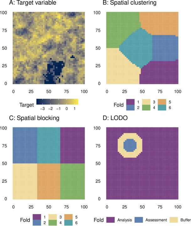
The final spatial CV method investigated here is leave-one-disc-out CV, following Brenning (2012). This method extends BLO3 by adding all points within a certain radius of each observation to $D_{\operatorname{out}}$, increasing the size of the final $D_{\operatorname{out}}$. Data points falling within the exclusion buffer of any observation in $D_{\operatorname{out}}$, including those added by the inclusion radius, is then removed from $D_{\operatorname{out}}$ (Figure 1). Similarly to blocked and clustered CV, LODO CV evaluates models against multiple $D_{\operatorname{out}}$ of spatially conjunct observations. Similar to BLO3 CV, LODO CV approach may be more robust to different parameter values than methods assigning $D_{\operatorname{out}}$ based upon blocking polygons or cluster boundaries. Unlike any of the other approaches investigated, observations may appear in multiple $D_{\operatorname{out}}$, with observations in more intensively sampled regions being selected more often.

In this study, spatial leave-one-disc-out CV was performed using the spatial_buffer_vfold_cv() function in spatialsample. An important feature of this implementation of leave-disc-out CV is that the exclusion buffer is calculated separately for each point in $D_{\operatorname{out}}$. Where other implementations remove all observations within the buffer distance of the inclusion radius to create a uniform “doughnut” shaped buffer, spatialsample only removes observations that are within the buffer distance of data in $D_{\operatorname{out}}$, potentially retaining more data in $D_{\operatorname{in}}$ by creating an irregular buffer polygon.

4 Methods

4.1 Landscape Simulation

To compare the validation techniques described above, we extended the simulation approach used by Roberts et al. (2017, Box 1). We simulated 100 landscapes, representing independent realizations of the same data-generating process, generating a set of 13 variables calculated using the same stochastic formulations across a regularly spaced 50 x 50 cell grid, for a total of 2,500 cells per landscape (Table 1). Simulated predictors included eight random Gaussian fields, generated using the RandomFields R package (Schlather et al. 2015), which uses stationary isotropic covariance models to generate spatially structured variables. Five additional variables were calculated as combinations of the randomly generated variables to imitate interactions between environmental variables. This simulation approach was originally designed to resemble the environmental data that might be used to model species abundance and distribution; further interpretation of what each predictor represents is provided in Appendix 2 of Roberts et al. (2017).

Table 1: Simulated predictors generated for each independent landscape, created following Roberts et al. 2017. Predictors are indicated as being used for y if they were included either in Equation 1 or used to calculate variables included in Equation 1. Predictors are indicated as being used in models if they were used as predictors in random forest models.

Name	Variable Definition	Used for $y$?	Used in model?
X1	Random Gaussian field with exponential covariance (variance = 0.1, scale = 0.1)	Yes	No
X2	Random Gaussian field with exponential covariance (variance = 0.3, scale = 0.1)	No	Yes
X3	Random Gaussian field with Gaussian covariance (variance = 0.1, scale = 0.3)	No	Yes
X4	If the ratio (X2 / X3) is above the 95th percentile of all values, 0; else 1.	Yes (excluding)	No
X5	X1 + X2 + X3 + (X2 $\cdot$ X3)	Yes	No
X6	Random Gaussian field with exponential covariance (variance = 0.1, scale = 0.1)	Yes	Yes
X7	Random Gaussian field with exponential covariance (variance = 0.1, scale = 0.1)	No	Yes
X8	Random Gaussian field with exponential covariance (variance = 0.1, scale = 0.1)	No	Yes
X9	Random Gaussian field with Gaussian covariance (variance = 0.1, scale = 0.3)	No	Yes
X10	Random Gaussian field with Gaussian covariance (variance = 0.1, scale = 0.3)	No	Yes
X11	X2/X3	Yes (limiting)	No
X12	$1/(\operatorname{sqrt}(2\cdot\pi))\cdot\exp-(\operatorname{X3}^{2}/4)$	Yes	No
X13	$1/(\operatorname{sqrt}(2\cdot\pi))\cdot\exp-(\operatorname{X2}^{2}/4)$	Yes	No

These predictors were then used to generate a target variable $y$ using Equation 1.

$$\hypertarget{eq-y}{}{y=\left\{\begin{array}[]{lr}\min(y),&\text{if }\operatorname{X4}\neq 0\\ \operatorname{X11},&\text{if }y\geq\operatorname{X11}\\ \operatorname{X1}+\operatorname{X5}+\operatorname{X6}+\operatorname{X12}+\operatorname{X13},&\text{otherwise }\end{array}\right\}}$$ (1)

One instance of the spatially clustered $y$ values produced by this process is visualized in Figure 1.

Figure 1: One simulation of the dependent variable $y$ and several of the CV approaches used. A: Simulated data showing environmental clustering of a variable of interest, named “Target”, in one simulated landscape. B: Spatial clustering CV fold assignments, as produced by spatial_clustering_cv(), based upon using k-means clustering to group observations spatially. C: Spatially blocked CV fold assignments, produced using spatial_block_cv() to group observations spatially. D: A single fold of LODO CV, showing $D_{\operatorname{in}}$ and $D_{\operatorname{out}}$ as well as the exclusion buffer, performed using spatial_buffer_vfold_cv() with a radius and buffer covering 10% of the mapped area. Points within the inclusion radius of the randomly selected observation are included in $D_{\operatorname{out}}$, while points within the exclusion buffer of $D_{\operatorname{out}}$ are not included in either set. For BLO3 and LODO CV, this procedure is repeated for each grid cell.

Models were then fit using variables X2, X3, and X6 - X10. Of these seven variables, three were involved in calculating the target variable $y$ (X2 and X3, as components of X4 and X5; and X6, used directly) and therefore provide useful information for models, while the remaining four (X7 - X10) were included to allow overfitting.

4.2 Resampling Methodology

We divided each simulated landscape into folds using each of the data splitting approaches (Section 3) across a wide range of parameter sets (Table 2; Table 3) in order to evaluate the usefulness of spatial CV approaches. Spatial blocking, spatial clustering, and leave-one-disc-out used a “leave-one-group-out” approach, where each $D_{\operatorname{out}}$ was made up of a single block or cluster of observations, with all other data (excluding any within the exclusion buffer) used as $D_{\operatorname{in}}$. BLO3 used a leave-one-observation-out approach. We additionally evaluated spatial blocking with fewer $D_{\operatorname{out}}$ than blocks, resulting in multiple blocks being used in each $D_{\operatorname{out}}$. Each simulated landscape was resampled independently, meaning that stochastic methods (such as V-fold CV and spatial clustering) produced different CV folds across each simulation. All resampling used functions implemented in the rsample and spatialsample packages (Frick et al. 2022; Mahoney and Silge 2022). Examples of spatial clustering CV, spatially blocked CV, and leave-one-disc-out CV are visualized in Figure 1.

Table 2: Parameters applied to each CV method assessed, and the number of iterations performed. 100 iterations were performed per unique combination of parameters.

CV Method Resampling function Parameters # of iterations Resubstitution 100 V-fold vfold_cv() V 400 Blocked spatial_block_cv() Block size, Buffer 8800 Clustered spatial_clustering_cv() V, Buffer, Cluster function 8800 BLO3 spatial_buffer_vfold_cv() Buffer 1700 LODO spatial_buffer_vfold_cv() Buffer, Radius 11100

Table 3: Definitions of parameters applied to CV methods.

Parameter	Values	Definition
V	2, 5, 10, 20; 2, 4, 9, 16, 25, 36, 64, 100	The number of folds to assign data into. Each fold was used as $D_{\operatorname{out}}$ precisely once. The first set of values were used for spatial clustering, while the second was used for spatial blocking. For spatial clustering, this controls the number of clusters.
Cluster function	K-means, Hierarchical	The algorithm used to cluster observations into folds.
Block size	1/100, 1/64, 1/36, 1/25, 1/16, 1/9, 1/4, 1/2	The proportion of the grid each block should occupy (such that 1/2 creates two blocks, each occupying half the grid).
Blocking method	Random, Systematic (continuous), Systematic (snake)	For spatial blocking, the method for assigning blocks to folds: randomly (’random’), in a ’scanline’ moving left to right across each row of the grid (’systematic (continuous)’), or moving back and forth across the rows of the grid (’systematic (snake)’).
Buffer	0.00, 0.03, 0.06, 0.09, 0.12, 0.15, 0.18, 0.21, 0.24, 0.27, 0.30, 0.33, 0.36, 0.39, 0.42, 0.45, 0.48	The size of the exclusion buffer to apply around $D_{\operatorname{out}}$, expressed as a proportion of the side length of the grid. Observations within this distance of any point in $D_{\operatorname{out}}$ are included in neither $D_{\operatorname{in}}$ nor $D_{\operatorname{out}}$. Buffer distances above 0.3 were only used for BLO3 CV, as increased buffer distances around larger $D_{\operatorname{out}}$ may produce empty $D_{\operatorname{in}}$.
Radius	0.00, 0.03, 0.06, 0.09, 0.12, 0.15, 0.18, 0.21, 0.24, 0.27, 0.30	The size of the inclusion radius to apply around $D_{\operatorname{out}}$, expressed as a proportion of the side length of the grid. Observations within this distance of any point in $D_{\operatorname{out}}$ are moved from $D_{\operatorname{in}}$ into $D_{\operatorname{out}}$.

4.3 Model Fitting and Evaluation

For each iteration, we modeled the target variable $y$ using random forests as implemented in the ranger R package (Breiman 2001; Wright and Ziegler 2017), fit using variables X2, X3, and X6 - X10. Random forests generally provide high predictive accuracy even without hyperparameter tuning (Probst, Bischl, and Boulesteix 2018), and as such all random forests were fit using the default hyperparameter settings of the ranger package, namely 500 decision trees, a minimum of 5 observations per leaf node, and two variables to split on per node.

Model accuracy was measured using root-mean-squared error (RMSE, Equation 2). To find the “ideal” error rate that we would expect CV approaches to estimate, we fit 100 separate random forest models, each trained using all values within one of the 100 simulated landscapes. We then calculated the RMSE for each of these models when used to predict each of the 99 other landscapes. As each landscape is an independent realization of the same data-generation process, the relationships between predictors and $y$ is identical across landscapes, although the spatial relationships between $y$ and variables not used to generate $y$ are likely different across iterations. As such, RMSE values from a model trained on one landscape and used to predict the others represent the ability of the model to predict $y$ based upon the predictors and without relying upon spatial structure. These RMSE estimates therefore represent the “true” range of RMSE values when using these models for spatial extrapolation to areas with the same relationship between predictors and the target feature, but without any spatial correlation to the training data itself. We defined the success of model evaluation methods as the proportion of iterations which returned RMSE estimates between the 5th and 9th percentile RMSEs of this “ideal” estimation procedure.

To find the error rate of the resubstitution approach, we fit 100 random forests, one to each landscape, and then calculated the RMSE for each model when used to predict its own training data. To find the error of each CV approach, we first used each CV approach to separate each landscape into $n$ folds (Section 4.2). We then fit models to each combination of $n-1$ of these folds, and calculated RMSE when using the model to predict the remaining $D_{\operatorname{out}}$ (Equation 2).

$$\hypertarget{eq-rmse}{}{\operatorname{RMSE}=\sqrt{(\frac{1}{n})\sum_{i=1}^{n}(y_{i}-\hat{y_{i}})^{2}}}$$ (2)

We then calculated the variance of the RMSE estimates of each method across the 100 simulated landscapes, as well as the proportion of runs for each method which fell between the 5th and 95th percentiles of the “true” RMSE range.

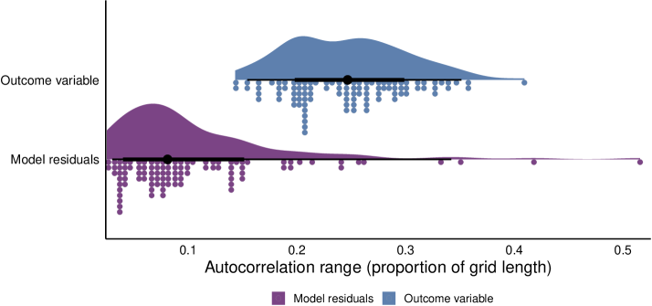
Based upon prior research, we expected the optimal spacing between $D_{\operatorname{in}}$ and $D_{\operatorname{out}}$ to be related to the range of spatial dependence either in the outcome variable or in model residuals (Le Rest et al. 2014; Roberts et al. 2017; Telford and Birks 2009). As such, we quantified the range of spatial autocorrelation in both the target variable $y$ and in resubstitution residuals from random forest models using the automated variogram fitting approach implemented in the automap R package (Hiemstra et al. 2008).

5 Results and Discussion

5.1 Spatial CV Improves Model Performance Estimates

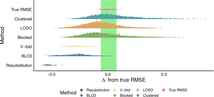
Spatial cross-validation methods consistently produced more accurate estimates of model performance than non-spatial methods, which were optimistically biased (producing too-low estimates of RMSE) (Table 4; Figure 2). CV produced the best estimates when $D_{\operatorname{out}}$ of spatially conjunct observations were combined with exclusion buffers (Table 5). Spatially clustered CV and LODO, both of which enforce $D_{\operatorname{out}}$ of spatially conjunct observations, were among the most consistently effective CV methods (Figure 2). Removing too much data from $D_{\operatorname{in}}$, such as by clustering with only two folds or blocking with only two blocks resulted in pessimistic over-estimates of RMSE (Figure 3).

Table 4: Mean RMSE estimates across all evaluated parameterizations of cross-validation strategies. Numbers in parentheses represent standard deviations. “% within target RMSE range” refers to the percentage of iterations which had RMSE estimates between the 5th and 95th percentile estimates from the true RMSE estimation procedure.

Method	RMSE	% within target RMSE range
Ideal RMSE	0.715 (0.042)	90.00%
Clustered	0.743 (0.161)	36.97%
LODO	0.641 (0.135)	31.70%
Blocked	0.664 (0.159)	27.90%
V-fold	0.440 (0.076)	2.00%
BLO3CV	0.429 (0.098)	1.29%
Resubstitution	0.189 (0.032)	0.00%

Figure 2: RMSE distributions of each spatial CV method evaluated. The x axis represents the distance of an RMSE from the mean “true” RMSE values, such that negative values underpredict the true RMSE and positive values overpredict it. Distributions are scaled relative to the number of iterations run, such that a unit area represents the same number of iterations across each method, but not necessarily the same proportion of all iterations evaluated. The green rectangle represents the 90% interval of true RMSE values used as the “target” RMSE range.

Table 5: Mean RMSE estimates across 100 iterations of various cross-validation strategies (bold headers) for the parameterizations producing the most accurate model performance estimates. Numbers in parentheses represent standard deviations. “% within target RMSE range” refers to the percentage of iterations which had RMSE estimates between the 5th and 95th percentile estimates from the true RMSE estimation procedure.

V	Cell size	Cluster function	Exclusion buffer	Inclusion radius	RMSE	% within target RMSE range
Ideal RMSE
					0.715 (0.042)	90.00%
Clustered
10		kmeans	0.15		0.694 (0.087)	60.00%
5		kmeans	0.09		0.723 (0.099)	59.00%
10		kmeans	0.18		0.712 (0.094)	59.00%
LODO
			0.18	0.21	0.718 (0.095)	60.00%
			0.12	0.24	0.703 (0.093)	59.00%
			0.12	0.27	0.725 (0.098)	59.00%
Blocked
	1/9		0.24		0.738 (0.099)	61.00%
	1/9		0.21		0.732 (0.100)	60.00%
	1/25		0.27		0.688 (0.084)	58.00%
V-fold
2					0.475 (0.079)	2.00%
5					0.438 (0.073)	2.00%
10					0.428 (0.071)	2.00%
BLO3
			0.48		0.524 (0.070)	7.00%
			0.45		0.516 (0.069)	4.00%
			0.42		0.508 (0.067)	3.00%
Resubstitution
					0.189 (0.032)	0.00%

Figure 3: Spatial CV RMSE estimates under various parameterizations. Colors represent the distance of an RMSE from the mean “true” RMSE values, such that negative values underpredict the true RMSE and positive values overpredict it. A: Spatial clustering RMSE estimates using different numbers of clusters (“V”) and different sizes of exclusion buffers (“Buffer”). B: Spatial blocking RMSE estimates using different sizes of blocks (“Cell Size”; a cell size of “1/2” implies two blocks, each containing half the study area) and different sizes of exclusion buffers (“Buffer”). C: LODO RMSE estimates using different sizes of inclusion radii (“Radius”) and different sizes of exclusion buffers (“Buffer”). D: BLO3 RMSE estimates using different sizes of exclusion buffers (“Buffer”).

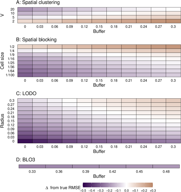
The best parameter sets for CV methods consistently separated the center of $D_{\operatorname{out}}$ from $D_{\operatorname{in}}$ by 25%-41% of the grid length (Clustering 25%-29%; LODO 36%-39%; Blocked 32%-41%; BLO3 24%-30%). Given that the target variable had a mean autocorrelation range of 24.61% of the grid length (Figure 4), this suggests that spatial cross-validation approaches produce the best estimates of model performance when $D_{\operatorname{out}}$ is sufficiently separated from $D_{\operatorname{in}}$ such that there is no spatial dependency in the outcome variable between the two sets.

Figure 4: Autocorrelation range distributions for the outcome variable and resubstitution model residuals, used throughout the literature to identify target distances to separate $D_{\operatorname{out}}$ and $D_{\operatorname{in}}$. Units are as a proportion of the side length of the grid. Ranges were determined via empirical variogram. Each point represents one iteration of the simulation process, while “clouds” represent the matching probability density function. Black points represent the median autocorrelation range, while the black bar represents the interquartile range and 95% interval.

Clustering appeared to be the spatial CV method most robust to different parameterizations (Figure 2; Figure 3), with the highest proportion of all iterations within the target RMSE range (Clustered 36.97% of all iterations; LODO 31.70%; Blocked 27.90%; BLO3 ) (Figure 5). This may, however, simply reflect the relatively narrow range of parameters evaluated with clustering, as both blocking and LODO had a wide range of parameters which returned estimates within the target range at least half the time (Figure 5). While BLO3 exhibited increasing RMSE with increasing buffer radii (Figure 3), as frequently reported in the literature, we found it only rarely produced RMSE estimates within the target range (Figure 5).

Figure 5: Percentage of RMSE estimates within the target range (the 90% interval of true RMSE values) from spatial CV methods under various parameterizations. A: Spatial clustering using different numbers of clusters (“V”) and different sizes of exclusion buffers (“Buffer”). B: Spatial blocking using different sizes of blocks (“Cell Size”; a cell size of “1/2” implies two blocks, each containing half the study area) and different sizes of exclusion buffers (“Buffer”). C: LODO using different sizes of inclusion radii (“Radius”) and different sizes of exclusion buffers (“Buffer”). D: BLO3 using different sizes of exclusion buffers (“Buffer”).

RMSE estimates from spatial blocking were inversely related to the number of $D_{\operatorname{out}}$ used, likely due to the distance between $D_{\operatorname{out}}$ and $D_{\operatorname{in}}$ increasing if adjacent blocks were assigned to the same $D_{\operatorname{out}}$ (Figure 6). RMSE estimates generally increased gradually as the number of $D_{\operatorname{out}}$ decreased, though notable increases were observed when blocks were assigned via the continuous systematic method and the number of cells in each grid row were evenly divisible by the number of $D_{\operatorname{out}}$ (e.g., when 1/16th cell sizes produced by a 4-by-4 grid were divided into 4 folds). In these situations, each column of the grid will be entirely assigned to the same $D_{\operatorname{out}}$, somewhat resembling the CV method of Wenger and Olden (2012), producing $D_{\operatorname{out}}$ which have no neighboring $D_{\operatorname{in}}$ observations in the y direction and therefore a greater average distance between $D_{\operatorname{out}}$ and $D_{\operatorname{in}}$. Overall, these results suggest that using fewer $D_{\operatorname{out}}$ than blocks may be appropriate when the range of autocorrelation in the outcome variable is relatively small and there is concern about large blocks restricting predictor space (Roberts et al. 2017); however, with longer autocorrelation ranges it is likely best to use a leave-one-block-out approach with fewer, larger blocks.

Figure 6: RMSE estimates from spatially blocked CV with various block sizes assigned to various numbers of $D_{\operatorname{out}}$. A: Spatial CV RMSE estimates under various parameterizations. Colors represent the distance of an RMSE from the mean “true” RMSE values, such that negative values underpredict the true RMSE and positive values overpredict it. B: Percentage of RMSE estimates within the target range (the 90% interval of true RMSE values). Labels above each panel refer to the method for assigning blocks to folds: either random assignment, systematically with each row assigned from left to right (“continuous”), or systematically with each row assigned in a “snaking” pattern (first row left to right, next row right to left, then repeating).

As such, the recommendations from this study are clear: CV-based performance assessments of models fit using spatial data benefit from spatial CV approaches. Those spatial CV approaches are most likely to return good estimates of true model accuracy if they combine $D_{\operatorname{out}}$ of spatially conjunct observations with exclusion buffers, such that the average observation is separated from $D_{\operatorname{in}}$ by enough distance that there is no spatial dependency in the outcome variable between $D_{\operatorname{in}}$ and $D_{\operatorname{out}}$.

5.2 Limitations

This simulation study assumed that spatial CV could take advantage of regularly distributed observations, such that all locations had a similar density of measurement points. This assumption is often violated, as it is often impractical to obtain a uniform sample across large areas, and as such observations are often clustered in more convenient locations and relatively sparse in less accessible areas (Meyer and Pebesma 2022; Martin, Blossey, and Ellis 2012). Alternative approaches not investigated in this study may be more effective in these situations; for instance, when the expected distance between training data and model predictions is known, Milà et al. (2022) proposes an alternative nearest neighbor distance matching CV approach which may equal or improve upon buffered leave-one-out CV. An alternative approach put forward by Meyer et al. (2018) uses meaningful, human-defined locations as groups for CV, which may produce better results than the automated partitioning methods investigated in this study. While we believe our results clearly demonstrate the benefits of spatial CV for sampling designs resembling our simulation, we do not pretend to present the one CV approach to rule them all.

We additionally do not expect these results, focused upon using CV to evaluate the accuracy of predictive models, will necessarily transfer to map accuracy assessments. Stehman and Foody (2019) explained that design-based sampling approaches provide unbiased assessments of map accuracy, while Wadoux et al. (2021) demonstrated that spatial CV methods may be overly pessimistic when assessing map accuracy, and Bruin et al. (2022) suggested sampling-intensity weighted CV approaches for map accuracy assessments in situations where the study area has been unevenly sampled. However, we expect these results will be informative in the many situations requiring estimates of model accuracy, particularly given that traditional held-out test sets are somewhat rare in the spatial modeling literature.

Lastly, we did not investigate any CV approaches which aim to preserve outcome or predictor distributions across $D_{\operatorname{out}}$. When working with imbalanced outcomes, random sampling may produce $D_{\operatorname{out}}$ with notably different outcome distributions than the overall training data, which may bias performance estimates. Assigning stratified samples of observations to $D_{\operatorname{out}}$ can address this, but it is not obvious how to use stratified sampling when assigning groups of observations (such as a spatial cluster or block), with one outcome value per observation, to $D_{\operatorname{out}}$ as a unit. The rsample package allows stratified CV when all observations within a given group have identical outcome values (that is, when groups are strictly nested within the stratification variable), but this condition is rare and difficult to enforce when using unsupervised group assignment based on spatial location, as with all the spatial CV methods we investigated.

Creating $D_{\operatorname{out}}$ based on predictor space, rather than outcome distributions, has also been proposed as a solution to spatial CV procedures restricting the predictor ranges present in $D_{\operatorname{in}}$. This is a particular challenge if the predictors themselves are spatially structured, and may unintentionally force models to extrapolate further in predictor space than would be expected when predicting new data (Roberts et al. 2017). As increasing distance in predictor space often correlates with increasing error (e.g. Thuiller et al. 2004; Sheridan et al. 2004; Meyer and Pebesma 2021), Roberts et al. (2017) suggest blocking approaches to minimize distance in predictor space between folds, although to the best of our knowledge these approaches are not yet in widespread use. A related field of research suggests methods for calculating the applicability domain of a model (Netzeva et al. 2005; Meyer and Pebesma 2021), which can help to identify when predicting new observations will require extrapolation in predictor space, and will likely produce predictions with higher than expected errors. Such methods are particularly well-equipped to supplement spatial CV procedures, as it adjusts the permissible distance in predictor space based upon the distance between $D_{\operatorname{in}}$ and $D_{\operatorname{out}}$.

6 Conclusion

These results reinforce that spatial CV is essential for evaluating the performance of predictive models fit to data with internal spatial structure, particularly in situations where design-based map accuracy assessments are not practical or germane. Techniques that apply exclusion buffers around assessment sets of spatially conjunct observations, such as spatial clustering and LODO, are likely to produce the best estimates of model performance. The most accurate estimates of model performance are produced when the assessment and analysis data are sufficiently separated so that there is no spatial dependence in the outcome variable between the two sets.

7 Acknowledgements

We would like to thank Posit, PBC, for support in the development of the rsample and spatialsample packages.

8 Software, data, and code availability

The spatialsample package is available online at https://github.com/tidymodels/spatialsample . All data and code used in this paper are available online at https://github.com/cafri-labs/assessing-spatial-cv .

References

reAdams, Matthew D., Felix Massey, Karl Chastko, and Calvin Cupini. 2020. “Spatial Modelling of Particulate Matter Air Pollution Sensor Measurements Collected by Community Scientists While Cycling, Land Use Regression with Spatial Cross-Validation, and Applications of Machine Learning for Data Correction.” Atmospheric Environment 230 (June): 117479. https://doi.org/10.1016/j.atmosenv.2020.117479.

preBahn, Volker, and Brian J. McGill. 2012. “Testing the Predictive Performance of Distribution Models.” Oikos 122 (3): 321–31. https://doi.org/10.1111/j.1600-0706.2012.00299.x.

preBastin, Jean-Francois, Yelena Finegold, Claude Garcia, Danilo Mollicone, Marcelo Rezende, Devin Routh, Constantin M. Zohner, and Thomas W. Crowther. 2019. “The Global Tree Restoration Potential.” Science 365 (6448): 76–79. https://doi.org/10.1126/science.aax0848.

preBates, Stephen, Trevor Hastie, and Robert Tibshirani. 2021. “Cross-Validation: What Does It Estimate and How Well Does It Do It? arXiv:2104.00673v2 [Stat.ME].” https://doi.org/10.48550/arXiv.2104.00673.

preBreiman, Leo. 2001. “Random Forests.” Machine Learning 45: 5–32. https://doi.org/10.1023/A:1010933404324.

preBrenning, Alexander. 2012. “Spatial Cross-Validation and Bootstrap for the Assessment of Prediction Rules in Remote Sensing: The R Package sperrorest.” 2012 IEEE International Geoscience and Remote Sensing Symposium, July. https://doi.org/10.1109/igarss.2012.6352393.

preBruin, Sytze de, Dick J. Brus, Gerard B. M. Heuvelink, Tom van Ebbenhorst Tengbergen, and Alexandre M.J-C. Wadoux. 2022. “Dealing with Clustered Samples for Assessing Map Accuracy by Cross-Validation.” Ecological Informatics 69 (July): 101665. https://doi.org/10.1016/j.ecoinf.2022.101665.

preBrus, Dick J. 2020. “Statistical Approaches for Spatial Sample Survey: Persistent Misconceptions and New Developments.” European Journal of Soil Science 72 (2): 686–703. https://doi.org/10.1111/ejss.12988.

preDunnington, Dewey, Edzer Pebesma, and Ege Rubak. 2021. s2: Spherical Geometry Operators Using the S2 Geometry Library. https://CRAN.R-project.org/package=s2.

preEfron, Bradley. 1986. “How Biased Is the Apparent Error Rate of a Prediction Rule?” Journal of the American Statistical Association 81 (394): 461–70. https://doi.org/10.1080/01621459.1986.10478291.

preEfron, Bradley, and Gail Gong. 1983. “A Leisurely Look at the Bootstrap, the Jackknife, and Cross-Validation.” The American Statistician 37 (1): 36–48. https://doi.org/10.1080/00031305.1983.10483087.

preFick, Stephen E., and Robert J. Hijmans. 2017. “WorldClim 2: New 1-Km Spatial Resolution Climate Surfaces for Global Land Areas.” International Journal of Climatology 37 (12): 4302–15. https://doi.org/10.1002/joc.5086.

preFrick, Hannah, Fanny Chow, Max Kuhn, Michael Mahoney, Julia Silge, and Hadley Wickham. 2022. rsample: General Resampling Infrastructure. https://CRAN.R-project.org/package=rsample.

preGong, Gail. 1986. “Cross-Validation, the Jackknife, and the Bootstrap: Excess Error Estimation in Forward Logistic Regression.” Journal of the American Statistical Association 81 (393): 108–13. https://doi.org/10.1080/01621459.1986.10478245.

preGruijter, J. J. de, and C. J. F. ter Braak. 1990. “Model-Free Estimation from Spatial Samples: A Reappraisal of Classical Sampling Theory.” Mathematical Geology 22 (4): 407–15. https://doi.org/10.1007/bf00890327.

preHengl, Tomislav, Jorge Mendes de Jesus, Gerard B. M. Heuvelink, Maria Ruiperez Gonzalez, Milan Kilibarda, Aleksandar Blagotić, Wei Shangguan, et al. 2017. “SoilGrids250m: Global Gridded Soil Information Based on Machine Learning.” Edited by Ben Bond-Lamberty. PLOS ONE 12 (2): e0169748. https://doi.org/10.1371/journal.pone.0169748.

preHiemstra, P. H., E. J. Pebesma, C. J. W. Twenhöfel, and G. B. M. Heuvelink. 2008. “Real-Time Automatic Interpolation of Ambient Gamma Dose Rates from the Dutch Radioactivity Monitoring Network.” Computers & Geosciences. https://doi.org/10.1016/j.cageo.2008.10.011.

preHoogen, Johan van den, Stefan Geisen, Devin Routh, Howard Ferris, Walter Traunspurger, David A. Wardle, Ron G. M. de Goede, et al. 2019. “Soil Nematode Abundance and Functional Group Composition at a Global Scale.” Nature 572 (7768): 194–98. https://doi.org/10.1038/s41586-019-1418-6.

preKarasiak, N., J.-F. Dejoux, C. Monteil, and D. Sheeren. 2021. “Spatial Dependence Between Training and Test Sets: Another Pitfall of Classification Accuracy Assessment in Remote Sensing.” Machine Learning 111 (7): 2715–40. https://doi.org/10.1007/s10994-021-05972-1.

preKuhn, Max. 2022. tune: Tidy Tuning Tools. https://CRAN.R-project.org/package=tune.

preKuhn, Max, and Hannah Frick. 2022. dials: Tools for Creating Tuning Parameter Values. https://CRAN.R-project.org/package=dials.

preKuhn, Max, and Kjell Johnson. 2013. Applied Predictive Modeling. Vol. 26. Springer. https://doi.org/10.1007/978-1-4614-6849-3.

pre———. 2019. Feature Engineering and Selection. Chapman; Hall/CRC. https://doi.org/10.1201/9781315108230.

preKuhn, Max, and Julia Silge. 2022. Tidy Modeling with R. O’Reilly.

preLe Rest, Kévin, David Pinaud, Pascal Monestiez, Joël Chadoeuf, and Vincent Bretagnolle. 2014. “Spatial Leave-One-Out Cross-Validation for Variable Selection in the Presence of Spatial Autocorrelation.” Global Ecology and Biogeography 23 (7): 811–20. https://doi.org/10.1111/geb.12161.

preLegendre, Pierre, and Marie Josée Fortin. 1989. “Spatial Pattern and Ecological Analysis.” Vegetatio 80 (2): 107–38. https://doi.org/10.1007/bf00048036.

preMahoney, Michael, and Julia Silge. 2022. spatialsample: Spatial Resampling Infrastructure. https://CRAN.R-project.org/package=spatialsample.

preMartin, Laura J, Bernd Blossey, and Erle Ellis. 2012. “Mapping Where Ecologists Work: Biases in the Global Distribution of Terrestrial Ecological Observations.” Frontiers in Ecology and the Environment 10 (4): 195–201. https://doi.org/10.1890/110154.

preMeyer, Hanna, and Edzer Pebesma. 2021. “Predicting into Unknown Space? Estimating the Area of Applicability of Spatial Prediction Models.” Methods in Ecology and Evolution 12 (9): 1620–33. https://doi.org/10.1111/2041-210x.13650.

pre———. 2022. “Machine Learning-Based Global Maps of Ecological Variables and the Challenge of Assessing Them.” Nature Communications 13 (1). https://doi.org/10.1038/s41467-022-29838-9.

preMeyer, Hanna, Christoph Reudenbach, Tomislav Hengl, Marwan Katurji, and Thomas Nauss. 2018. “Improving Performance of Spatio-Temporal Machine Learning Models Using Forward Feature Selection and Target-Oriented Validation.” Environmental Modelling & Software 101 (March): 1–9. https://doi.org/10.1016/j.envsoft.2017.12.001.

preMeyer, Hanna, Christoph Reudenbach, Stephan Wöllauer, and Thomas Nauss. 2019. “Importance of Spatial Predictor Variable Selection in Machine Learning Applications – Moving from Data Reproduction to Spatial Prediction.” Ecological Modelling 411 (November): 108815. https://doi.org/10.1016/j.ecolmodel.2019.108815.

preMilà, Carles, Jorge Mateu, Edzer Pebesma, and Hanna Meyer. 2022. “Nearest Neighbour Distance Matching Leave-One-Out Cross-Validation for Map Validation.” Methods in Ecology and Evolution 13 (6): 1304–16. https://doi.org/10.1111/2041-210x.13851.

preNetzeva, Tatiana I., Andrew P. Worth, Tom Aldenberg, Romualdo Benigni, Mark T. D. Cronin, Paola Gramatica, Joanna S. Jaworska, et al. 2005. “Current Status of Methods for Defining the Applicability Domain of (Quantitative) Structure-Activity Relationships.” Alternatives to Laboratory Animals 33 (2): 155–73. https://doi.org/10.1177/026119290503300209.

preO’Sullivan, David, and David J. Unwin. 2010. Geographic Information Analysis. John Wiley & Sons, Inc. https://doi.org/10.1002/9780470549094.

prePebesma, Edzer. 2018. “Simple Features for R: Standardized Support for Spatial Vector Data.” The R Journal 10 (1): 439–46. https://doi.org/10.32614/RJ-2018-009.

prePebesma, Edzer, Thomas Mailund, and James Hiebert. 2016. “Measurement Units in R.” R Journal 8 (2): 486–94. https://doi.org/10.32614/RJ-2016-061.

prePloton, Pierre, Frédéric Mortier, Maxime Réjou-Méchain, Nicolas Barbier, Nicolas Picard, Vivien Rossi, Carsten Dormann, et al. 2020. “Spatial Validation Reveals Poor Predictive Performance of Large-Scale Ecological Mapping Models.” Nature Communications 11 (1). https://doi.org/10.1038/s41467-020-18321-y.

prePohjankukka, Jonne, Tapio Pahikkala, Paavo Nevalainen, and Jukka Heikkonen. 2017. “Estimating the Prediction Performance of Spatial Models via Spatial k-Fold Cross Validation.” International Journal of Geographical Information Science 31 (10): 2001–19. https://doi.org/10.1080/13658816.2017.1346255.

preProbst, Philipp, Bernd Bischl, and Anne-Laure Boulesteix. 2018. “Tunability: Importance of Hyperparameters of Machine Learning Algorithms.” arXiv. https://doi.org/10.48550/ARXIV.1802.09596.

preR Core Team. 2022. R: A Language and Environment for Statistical Computing. Vienna, Austria: R Foundation for Statistical Computing. https://www.R-project.org/.

preRoberts, David R., Volker Bahn, Simone Ciuti, Mark S. Boyce, Jane Elith, Gurutzeta Guillera-Arroita, Severin Hauenstein, et al. 2017. “Cross-Validation Strategies for Data with Temporal, Spatial, Hierarchical, or Phylogenetic Structure.” Ecography 40 (8): 913–29. https://doi.org/https://doi.org/10.1111/ecog.02881.

preSchlather, Martin, Alexander Malinowski, Peter J. Menck, Marco Oesting, and Kirstin Strokorb. 2015. “Analysis, Simulation and Prediction of Multivariate Random Fields with Package RandomFields.” Journal of Statistical Software 63 (8): 1–25. https://doi.org/10.18637/jss.v063.i08.

preSchratz, Patrick, Jannes Muenchow, Eugenia Iturritxa, Jakob Richter, and Alexander Brenning. 2019. “Hyperparameter Tuning and Performance Assessment of Statistical and Machine-Learning Algorithms Using Spatial Data.” Ecological Modelling 406 (August): 109–20. https://doi.org/10.1016/j.ecolmodel.2019.06.002.

preSheridan, Robert P., Bradley P. Feuston, Vladimir N. Maiorov, and Simon K. Kearsley. 2004. “Similarity to Molecules in the Training Set Is a Good Discriminator for Prediction Accuracy in QSAR.” Journal of Chemical Information and Computer Sciences 44 (6): 1912–28. https://doi.org/10.1021/ci049782w.

preStehman, Stephen V., and Giles M. Foody. 2019. “Key Issues in Rigorous Accuracy Assessment of Land Cover Products.” Remote Sensing of Environment 231 (September): 111199. https://doi.org/10.1016/j.rse.2019.05.018.

preStone, M. 1974. “Cross-Validatory Choice and Assessment of Statistical Predictions.” Journal of the Royal Statistical Society. Series B (Methodological) 36 (2): 111–47. http://www.jstor.org/stable/2984809.

preTelford, R. J., and H. J. B. Birks. 2009. “Evaluation of Transfer Functions in Spatially Structured Environments.” Quaternary Science Reviews 28 (13-14): 1309–16. https://doi.org/10.1016/j.quascirev.2008.12.020.

preThuiller, Wilfried, Lluis Brotons, Miguel B. Araújo, and Sandra Lavorel. 2004. “Effects of Restricting Environmental Range of Data to Project Current and Future Species Distributions.” Ecography 27 (2): 165–72. https://doi.org/10.1111/j.0906-7590.2004.03673.x.

preTownsend, Peterson A., Monica Papeş, and Muir Eaton. 2007. “Transferability and Model Evaluation in Ecological Niche Modeling: A Comparison of GARP and Maxent.” Ecography 30 (4): 550–60. https://doi.org/10.1111/j.0906-7590.2007.05102.x.

preValavi, Roozbeh, Jane Elith, José J. Lahoz-Monfort, and Gurutzeta Guillera-Arroita. 2018. “blockCV: An R Package for Generating Spatially or Environmentally Separated Folds for k-Fold Cross-Validation of Species Distribution Models.” Edited by David Warton. Methods in Ecology and Evolution 10 (2): 225–32. https://doi.org/10.1111/2041-210x.13107.

preVarma, Sudhir, and Richard Simon. 2006. “Bias in Error Estimation When Using Cross-Validation for Model Selection.” BMC Bioinformatics 7 (1). https://doi.org/10.1186/1471-2105-7-91.

preWadoux, Alexandre M. J.-C., Gerard B. M. Heuvelink, Sytze de Bruin, and Dick J. Brus. 2021. “Spatial Cross-Validation Is Not the Right Way to Evaluate Map Accuracy.” Ecological Modelling 457 (October): 109692. https://doi.org/10.1016/j.ecolmodel.2021.109692.

preWalvoort, D. J. J., D. J. Brus, and J. J. de Gruijter. 2010. “An R Package for Spatial Coverage Sampling and Random Sampling from Compact Geographical Strata by k-Means.” Computers & Geosciences 36 (10): 1261–67. https://doi.org/10.1016/j.cageo.2010.04.005.

preWenger, Seth J., and Julian D. Olden. 2012. “Assessing Transferability of Ecological Models: An Underappreciated Aspect of Statistical Validation.” Methods in Ecology and Evolution 3 (2): 260–67. https://doi.org/10.1111/j.2041-210x.2011.00170.x.

preWickham, Hadley, Mara Averick, Jennifer Bryan, Winston Chang, Lucy McGowan, Romain François, Garrett Grolemund, et al. 2019. “Welcome to the Tidyverse.” Journal of Open Source Software 4 (43): 1686. https://doi.org/10.21105/joss.01686.

preWright, Marvin N., and Andreas Ziegler. 2017. “ranger: A Fast Implementation of Random Forests for High Dimensional Data in C++ and R.” Journal of Statistical Software 77 (1): 1–17. https://doi.org/10.18637/jss.v077.i01.

preYates, Katherine L., Phil J. Bouchet, M. Julian Caley, Kerrie Mengersen, Christophe F. Randin, Stephen Parnell, Alan H. Fielding, et al. 2018. “Outstanding Challenges in the Transferability of Ecological Models.” Trends in Ecology & Evolution 33 (10): 790–802. https://doi.org/10.1016/j.tree.2018.08.001.

p