Validation of uncertainty quantification metrics: a primer based on the consistency and adaptivity concepts

Abstract

The practice of uncertainty quantification (UQ) validation, notably in machine learning for the physico-chemical sciences, rests on several graphical methods (scattering plots, calibration curves, reliability diagrams and confidence curves) which explore complementary aspects of calibration, without covering all the desirable ones. For instance, none of these methods deals with the reliability of UQ metrics across the range of input features (adaptivity). Based on the complementary concepts of consistency and adaptivity, the toolbox of common validation methods for variance- and intervals- based UQ metrics is revisited with the aim to provide a better grasp on their capabilities. This study is conceived as an introduction to UQ validation, and all methods are derived from a few basic rules. The methods are illustrated and tested on synthetic datasets and representative examples extracted from the recent physico-chemical machine learning UQ literature.

I Introduction

The quest for confidence in the predictions of data-based algorithms(Vishwakarma2021, ; Gruich2023, ) has led to a profusion of uncertainty quantification (UQ) methods in machine learning (ML).(Pearce2018, ; Musil2019, ; Hirschfeld2020, ; Tran2020, ; Abdar2021, ; Gawlikowski2021, ; Tynes2021, ; Zelikman2021, ; Hu2022, ; Varivoda2022, ; He2023, ) Not all of these UQ methods provide uncertainties that can be relied on,(Liu2021, ; Pernot2022b, ) notably if one expects uncertainty to inform us on a range of plausible values for a predicted property.(GUM, ; Irikura2004, ) In pre-ML computational chemistry, UQ metrics consisted essentially in standard uncertainty, i.e. the standard deviation of the distribution of plausible values (a variance-based metric), or expanded uncertainty, i.e. the half-range of a prediction interval, typically at the 95 % level (an interval-based metric).(Ruscic2004, ; Irikura2004, ) The advent of ML methods provided UQ metrics beyond this standard setup, for instance distances in feature or latent space(Janet2019, ; Hullermeier2021, ; Hu2022, ) or the recent $\Delta$-metric,(Korolev2022, ) which have no direct statistical or probabilistic meaning. These metrics might however be converted to variance- or interval-based metrics by calibration methods, such as conformal inference.(Angelopoulos2021, ; Vovk2012, ) Still, all UQ metrics need to be validated to ensure that they are adapted to their intended use.

The validation of UQ metrics is designed around the concept of calibration. The use of uncertainty as a proxy to identify unreliable predictions, as done in active learning, does not require the same level of calibration as its use for the prediction of properties at the molecule-specific level.(Reiher2022, ) A handful of validation methods exist that explore more or less complementary aspects of calibration. A trio of methods seems to have recently taken the center-stage: the reliability diagram (or RMSE vs RMV plot), the calibration curve and the confidence curve. They implement three different approaches to calibration which are not necessarily independent, but they do not cover the full spectrum of calibration requirements. In particular, none of these methods addresses the essential reliability of predicted uncertainties with respect to the input features. As will be shown below, a UQ metric validated by this trio of methods might still be unreliable for individual predictions. Moreover, it appears that some methods are not always used in an appropriate context, such as the oracle confidence curve for variance-based UQ metrics.(Pernot2022c, )

The aim of this article is to design a principled validation framework based on complementary calibration concepts and review the relevant methods within this framework. The choice of methods is based on two main criteria: (1) the nature of the UQ metric to be validated (distribution, interval, variance, other…) and (2) the calibration target (average calibration, consistency or adaptivity, to be defined below).

I.1 Related studies

Most of the validation methods presented in this study derive from the seminal work of Gneiting et al.(Gneiting2007a, ; Gneiting2014, ) on the calibration of probabilistic forecasters. Probabilistic forecasters are models that provide for each prediction a distribution of plausible values. A major lesson from Gneiting’s work is that calibration metrics estimated over a validation dataset (average calibration) do not necessarily lead to useful UQ statements and that additional properties are necessary to design reliable UQ methods. An example is sharpness which quantifies the concentration of the prediction uncertainties: among a set of average-calibrated methods, one should prefer the sharpest one. Pernot(Pernot2022a, ) noted that, in the absence of a target value, sharpness might not be useful for the validation of individual UQ metrics, so that alternative statistics are required for UQ validation.

The definition of calibration provided by Gneiting et al. was extended by Kuleshov(Kuleshov2018, ). The formulation of Kuleshov, based on coverage probabilities, led to use calibration curves as a validation tool. But Levi et al.(Levi2020, ) demonstrated that calibration curves are not reliable and proposed instead to use individual calibration(Chung2020, ), based on the conditional variance of the errors with respect to the prediction uncertainty. Implementation of this conditional calibration equation led to reliability diagrams or RMSE vs RMV plots, also called calibration diagrams by Laves et al.(Laves2020, ). In practice, individual calibration is generally unreachable, and an alternative is to consider local calibration(Luo2021, ), which is reflected in the implementation of conditional statistics through binning schemes, as done for instance in reliability diagrams.

Pernot(Pernot2022b, ) proposed the concept of tightness to differentiate local calibration from average calibration, and implemented it in a Local Z-Variance (LZV) analysis in which calibration is estimated in subsets of the validation dataset. These subsets can be designed according to any relevant property (predicted value, uncertainty or input feature). He also established the link between LZV analysis in uncertainty space and reliability diagrams. Both reliability diagrams and LZV analysis derive from the concept of conditional calibration, but, for reliability diagrams, the conditioning variable is prediction uncertainty, while the LZV analysis opens a larger palette of conditioning variables. Conditional coverage with respect to input features was proposed by Vovk(Vovk2012, ) to asses the adaptivity(Angelopoulos2021, ) of conformal predictors. The adaptivity concept can therefore be linked to conditional calibration in input feature space, a form of tightness.

Confidence curves derive from another validation approach, known as sparsification error curves mainly used in computer vision.(Ilg2018, ; Scalia2020, ) They were not intended to validate calibration, but to estimate the correlation between absolute errors and UQ metrics.(Tynes2021, ) Pernot(Pernot2022c, ) showed that the standard reference curve (the so-called oracle) used for the evaluation of confidence curves is irrelevant for variance-based UQ metrics, and he introduced a new probabilistic reference that enables to test conditional calibration in uncertainty space.

Tran et al.(Tran2020, ) and Scalia et al.(Scalia2020, ) published motivating overviews of some of the methods presented here (reliability diagrams, calibration and confidence curves) applied to ML-UQ in materials sciences.

I.2 Contributions

Building on the the works of Levi et al.(Levi2020, ), Pernot(Pernot2022b, ) and Angelopoulos et al.(Angelopoulos2021, ) about conditional calibration, I propose to distinguish two calibration targets besides average calibration, namely

• consistency as the conditional calibration with respect to prediction uncertainty, and

• adaptivity as the conditional calibration with respect to input features.

Consistency derives from the metrological consistency of measurements,(Kacker2010, ) while adaptivity is borrowed from the conformal inference literature(Angelopoulos2021, ). Tightness, as introduced by Pernot(Pernot2022b, ), should then be understood as covering both consistency and adaptivity. Unless there is a monotonous transformation between input features and prediction uncertainty, consistency and adaptivity are distinct calibration targets.

The distinction between consistency and adaptivity is important to better define the objective(s) of each validation method. In fact, adaptivity has not been considered in recent overviews of ML-UQ validation metrics(Tran2020, ; Scalia2020, ), but was practically implemented – albeit unnamed – through the LZV and Local Coverage Probability (LCP) analyses (see for instance Fig. 4 in Pernot(Pernot2022a, )). Still, most ML-UQ validation studies focus on calibration and consistency, and I will show that this is not sufficient to ensure the reliability of an UQ method across the input features space. Adaptivity is essential to achieve reliable UQ at the molecule-specific level advocated by Reiher(Reiher2022, ).

I.3 Structure of the article

The theoretical bases of the calibration-consistency-adaptivity framework are presented in the next section (Sect. II) for variance- and interval-based UQ metrics. A comprehensive set of validation methods is reviewed next (Sect. III) according to their application range and calibration target, in order to appreciate their merits and limitations. Examples from the recent materials and chemistry ML-UQ literature are treated as case studies in Sect. IV. Recommendations are presented as conclusions (Sect. V).

II Validation concepts and models

A major distinction will be made below between variance-based UQ metrics and interval-based UQ metrics. These occur in ML as statistical summaries of empirical distributions or ensembles, or as parameters of theoretical distributions (typically normal). Other UQ metrics, such as distances in feature space or latent space,(Janet2019, ; Hu2022, ) or the $\Delta$-metric,(Korolev2022, ) which have not the correct dimension to be comparable to errors, need first to be converted to one of those two metrics to be usable for validation.(Vovk2012, ; Angelopoulos2021, ; Cauchois2021, ; Feldman2021, )

II.1 Validation model for variance-based UQ metrics

II.1.1 Validation datasets

In order to validate variance-based UQ results, one needs a set of predicted values $V=\{V_{i}\}_{i=1}^{M}$, the corresponding uncertainties $u_{V}=\{u{}_{V}\}_{i=1}^{M}$, reference data to compare with $R=\{R_{i}\}_{i=1}^{M}$, and possibly their uncertainties $u_{R}=\{u_{R_{i}}\}_{i=1}^{M}$. Most of the validation methods considered below require to transform these to $E=R-V$ and $u_{E}=(u_{R}^{2}+u_{V}^{2})^{1/2}$.

The minimal validation dataset, $C=\left\{E,u_{E}\right\}$, enables to test calibration and consistency but not adaptivity. It is therefore better to include a relevant input feature $X$ in the dataset $C=\left\{E,u_{E},X\right\}$, extending the validation targets to adaptivity in $X$ space. Alternatively, if validation is done a posteriori and no relevant input feature is available, adaptivity can be tested on $C=\left\{E,u_{E},V\right\}$, with some caveats presented in Sect. III.4.5.

II.1.2 Generative model

For variance-based UQ metrics, validation methods are based on a probabilistic model linking errors to uncertainties

$$E_{i}\sim D(0,u_{E_{i}})$$ (1)

where $D(\mu,\sigma)$ is an unspecified probability density function with mean $\mu$ and standard deviation $\sigma$. This model states that errors should be unbiased ($\mu=0$) and that uncertainty describes their dispersion as a standard deviation, following the metrological standard.(GUM, )

It is essential to note that the relation between $E$ and $u_{E}$ is asymmetric: small uncertainties should be associated with small errors, but small errors might be associated with small or large uncertainties, while large errors should be associated with large uncertainties. This considerably diminishes the interest of validation tests based on the ranking of $|E|$ vs $u_{E}$ (e.g. correlation coefficients).

II.1.3 Validation model

Average calibration.

According to the generative model, the validation of $u_{E}$ should be based on testing that it correctly describes the dispersion of $E$.(Pernot2022a, ; Pernot2022b, ) One can for instance check that

$$\mathrm{Var}(E)\simeq<u_{E}^{2}>$$ (2)

where the average is taken over the validation dataset, and which is valid only if $<E>\simeq 0$.(Pernot2022b, ) However, this formula ignores the pairing between errors and uncertainties, and a more stringent test is based on z-scores ($Z=E/u_{E}$)(Pernot2022b, ), i.e.

$$\mathrm{Var}(Z)\simeq 1$$ (3)

Note that if the elements of $E$ and $u_{E}$ are obtained as the means and standard deviations of small ensembles (say less than 30 elements) these formulas have to be transformed in order to account for the uncertainty on the statistics.(Pernot2022b, ) Unfortunately, hypotheses need then to be made on the distribution of these small ensembles. For a normal generative distribution of errors, the distribution of the mean of $n$ values (ensemble size) is a Student’s-t distribution with $\nu=n-1$ degrees of freedom, one should have $\mathrm{Var}(Z)\simeq(n-1)/(n-3)$.(Pernot2022b, )

The satisfaction of one or both of these tests (Eqns. 2-3) validates average calibration, which is a minimal requirement, but does not guarantee the usefulness of individual uncertainties, as average calibration can be satisfied by a compensation of under- and over-estimated values of $u_{E}$.

Conditional calibration: consistency and adaptivity.

Based on Eq. 3, one can evaluate the reliability of individual uncertainties by conditional calibration(Vovk2012, ; Angelopoulos2021, ), i.e.,

$$\mathrm{Var}(Z|A=a)\simeq 1,\,\forall a\in\mathcal{A}$$ (4)

where $A$ is a variable with values $a$ in $\mathcal{A}$. As detailed below, $A$ can be any relevant quantity, such as the uncertainty $u_{E}$ or a feature $X$. The choice of the conditioning variable depends on the question to be answered. Choosing the uncertainty $u_{E}$ will assess the calibration across the range of uncertainty values, i.e. the consistency between $E$ and $u_{E}$, while choosing $X$ will assess adaptivity.

Using this terminology, one can see that the individual calibration proposed by Levi et al.(Levi2020, )

$$\mathrm{Var}(E|u_{E}=\sigma)\simeq\sigma^{2},\,\forall\sigma>0$$ (5)

deriving from Eq. 2 validates consistency. Although it is a step forward from average calibration, it does not test the adaptivity of the UQ metric under scrutiny. Nor does the local Z-Variance (LZV) analysis(Pernot2022a, ; Pernot2022b, ) in $u_{E}$ space, which can be derived from Eq. 3

$$\mathrm{Var}(Z|u_{E}=\sigma)\simeq 1,\,\forall\sigma>0$$ (6)

Practical implementation of conditional calibration tests to variance- and interval- based UQ metrics requires to split the validation set into subsets, generally based on the binning of the conditioning variable. In these conditions, one is more testing local than individual calibration(Luo2021, ), and Eq. 5 leads to reliability diagrams(Levi2020, ), while Eq. 6 leads to the local Z-Variance (LZV) analysis in $u_{E}$ space. Note that the bin size in these methods should be small enough to get as close as possible to individual calibration, but also large enough to ensure a reasonable power for statistical testing. The LZV analysis is easily applicable to any conditioning variable (see examples in Pernot(Pernot2022a, )), which is not the case of the reliability diagram which would need to superimpose reliability curves for each subset and be difficult to analyze.

An ideal variance-based UQ metric, i.e., one which provides reliable individual uncertainties, should satisfy calibration, consistency and adaptivity. Consistency and adaptivity are therefore two complementary aspects of tightness, a term introduced in a previous study(Pernot2022b, ) to characterize local calibration.

Calibration is a necessary condition to reach consistency or adaptivity. In fact, consistency/adaptivity expressed as conditional calibration should imply average calibration, but the splitting of the data into subsets makes that the power of individual consistency/adaptivity tests is smaller than for the full validation set. It is therefore better to test average calibration separately, notably for small validation datasets. Note that for homoscedastic datasets ($u_{E}=c^{te}$) consistency is implied by calibration, but not adaptivity. As already mentioned, as $X$, $V$ and $u_{E}$ are not necessarily related by monotonous transformations, one should not expect these complementary conditional calibration tests to provide identical results.

II.2 Validation model for interval-based UQ metrics

Prediction intervals can be extracted from predictive distributions,(Gneiting2014, ) generated by quantile regression or conformal predictors,(Pearce2018, ; Hu2022, ) or estimated from a variance-based UQ metric and an hypothetical generative distribution(Pernot2022a, ).

II.2.1 Validation datasets

In order to validate interval-based UQ results, one needs a set of reference data $R=\{R_{i}\}_{i=1}^{M}$, and possibly their uncertainties $u_{R}=\{u_{R_{i}}\}_{i=1}^{M}$, and a series of prediction intervals with prescribed coverage $P$, $I_{V}=\{I_{V,P}=\{I_{V_{i},P}\}_{i=1}^{M}\}_{P\in\mathcal{P}}$, where $I_{V_{i},P}=[I_{V_{i},P}^{-},I_{V_{i},P}^{+}]$ and $\mathcal{P}$ is a set of coverage values, typically expressed as percentages in $]0,\thinspace 100[$.

For convenience and consistency with the variance-based approach, one might transform these data as errors and error intervals $C=\{V,I_{E}\}=\{V_{i},\{I_{E_{i},P}\}_{P\in\mathcal{P}}\}_{i=1}^{M}$ where $I_{E_{i},P}=[R_{i}-I_{V_{i},P}^{-},\thinspace R_{i}-I_{V_{i},P}^{+}]$ is the $P$ % interval for the prediction error at point $i$. As for variance-based UQ metrics, the uncertainty on the reference values, if any, should be accounted for, and the inclusion in the dataset of pertinent input features $X=\{X_{i}\}_{i=1}^{M}$ is necessary to test adaptivity.

II.2.2 Validation model

Average coverage.

Within this setup, a method is considered to be calibrated if prediction intervals have the correct empirical coverage. One defines the prediction interval coverage probability (PICP) as

$$\nu_{p}=\mathbb{P}\left(0\in I_{E,P}\right)$$ (7)

where $\mathbb{P}$ is the probability function, and $I_{E,P}$ is a $P=100p$ % prediction error interval. Using PICPs, a method is calibrated in average, or marginally, if

$$\nu_{p}=p,\,\forall 100p\in\mathcal{P}$$ (8)

which is equivalent to Kuleshov’s definition(Kuleshov2018, ) when all probability levels can be estimated (for instance if one has access to the full predictive distribution). For a limited set of probabilities, one gets a milder calibration constraint.

Application of Eq. 8 for a series of percentages provides a calibration curve, where the values of $\nu_{p}$ are plotted against the target probabilities $p$.(Kuleshov2018, )

Conditional coverage.

Average calibration based on PICPs can be met by validation sets with unsuitable properties(Levi2020, ), and, as for variance-based UQ metrics, it is possible to build more stringent calibration tests based on conditional coverage,(Angelopoulos2021, ) i.e.,

$$\nu_{p}=\mathbb{P}\left(0\in I_{E,P}|A=a\right),\thinspace\forall a\in\mathcal{A}$$ (9)

where $A$ is a property with values $a$ in $\mathcal{A}$. To get the analog of consistency, one might consider to use $U_{P}$, the half-range of $I_{E_{i},P}$, as a conditioning variable in order to check that errors are consistent at all uncertainty scales. For instance, Pernot used the expanded uncertainty $U_{95}$ to this aim.(Pernot2022a, ) For adaptivity testing, the conditioning variable can be any relevant feature $X$.(Pernot2022a, )

In practice, the PICPs are estimated as frequencies over the validation set

$$\nu_{p,M}=\frac{1}{M}\sum_{i=1}^{M}\boldsymbol{1}\left(0\in I_{E_{i},P}\right)$$ (10)

where $\boldsymbol{1}(x)$ is the indicator function for proposition $x$, taking values 1 when $x$ is true and 0 when $x$ is false. Estimating a PICP amounts to count the number of times prediction error intervals contain zero.

Implementation of the conditional coverage tests requites binning according to the conditioning variable, with PICP testing within each bin, leading to the Local Coverage Probability (LCP) analysis.(Pernot2022a, )

Note that, as for reliability diagrams it is also possible to consider conditional calibration curves, with the same problem of readability and interpretability of overlapping curves.

III Validation methods

The principles exposed in the previous section are now developed into practical methods grouped by validation target (average calibration, consistency and adaptivity). All methods are illustrated on synthetic datasets designed to reveal their potential limitations.

III.1 Synthetic datasets

To illustrate the methods presented in this study, six datasets of size $M=5000$ were designed to illustrate common validation problems. They are summarized in Table 1.

Case	Calibration	Consistency	Adaptivity
A	yes	yes	yes
B	yes	no	no
C	yes/no	no	no
D	no	no	no
E	yes	yes	yes
F	yes	-	no

Table 1: Summary of the validation properties expected from the synthetic datasets.

Case A features a quadratic model with additive heteroscedastic noise

$$R_{i} =a+X_{i}^{2}$$ (11)

$$u_{E_{i}} =b\times|R_{i}|$$ (12)

$$V_{i} =R_{i}+u_{E_{i}}\times N(0,1)$$ (13)

where $N(0,1)$ is the standard normal distribution. The errors are thus in agreement with the generative model (Eq. 1), and, by construction, the set $C=\{X,E,u_{E}\}$ is calibrated, consistent and adaptive. It should pass all the corresponding tests.

To generate a calibrated, non-consistent and non-adaptive dataset (Case B), one preserves all the data of Case A, except the uncertainties which are derived as perturbations of the mean uncertainty of Case A

$$u_{E_{i}}=\sqrt{<u_{E}>_{A}}\times N(1,0.1)$$ (14)

This transformation preserves the calibration, but the errors are now inconsistent with $u_{E}$ and adaptivity is also lost.

Case C is issued from Case A with a random ordering of $u_{E}$. This preserves average calibration by Eq. 2, but breaks calibration by Eq. 3. Consistency and adaptivity are also broken.

Case D is derived from Case A by a uniform scaling of $u_{E}$ by a factor two. This set should fail all the tests for calibration, consistency and adaptivity. Note that there is not much sense to test consistency and adaptivity when average calibration is not satisfied. This will be considered as illustrative of the expected diagnostics.

Case E is similar to Case A, but the errors have now a Student’s-$t_{\nu=4}$ distribution with four degrees of freedom

$$V_{i}=R_{i}+u_{E_{i}}\times t_{4}(0,1)$$ (15)

where $t_{4}(0,1)$ is the $t$ distribution scaled to have a unit variance. This dataset is calibrated, consistent and adaptive. However, tests involving a normality hypothesis for the generative distribution should fail.

Finally, Case F is an homoscedastic dataset deriving from Case A, where the uncertainties are replaced by a constant value (the root mean square of Case A uncertainties). It is calibrated, and not adaptive. For a homoscedastic dataset, consistency is identical to calibration.

III.2 Testing average calibration

The simplest way to assess average calibration for variance-based UQ metrics is to test the equality in Eq. 2 or in Eq. 3. Various statistical procedures have been proposed, and it is best to avoid any assumption of normality for the distribution of errors or z-scores. See Pernot(Pernot2022a, ) for details.

Application to the synthetic datasets is presented in Table 2. For Cases A, B, E and F, both tests are satisfied. Case D is obviously non calibrated. However, datasets with consistency problems (Case C) might still check one of both metrics.

	$\frac{\mathrm{Var}(E)}{<u_{E}^{2}>}$		$\mathrm{Var}(Z)$
Case A	0.	98	1.	02
Case B	0.	97	1.	02
Case C	0.	98	53.	8*
Case D	0.	25*	0.	26*
Case E	1.	09	0.	96
Case F	1.	00	1.	00

Table 2: Validation of average calibration for cases A-F. An asterisk (*) means that a statistic exceeds its admissible range.

For interval-based UQ metrics, validation is done by testing Eq. 8 for the probability levels that are available. The statistical procedure comes with the same caveats as for variance-based UQ metrics and has been detailed by Pernot(Pernot2022a, ). When a large set of probability levels is available, one can build a calibration curve, as shown next.

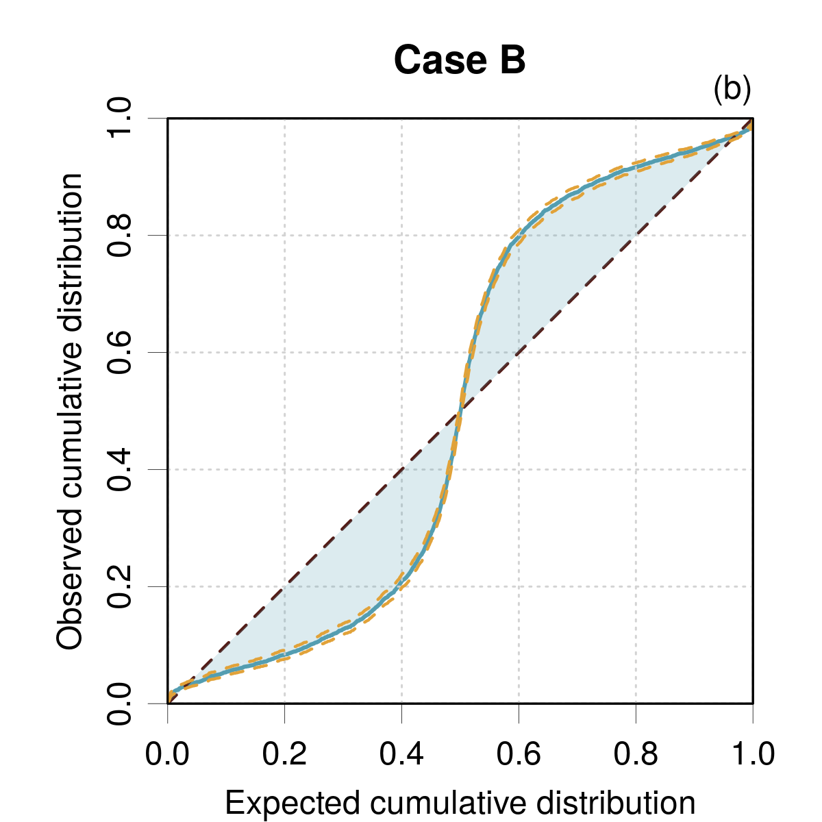
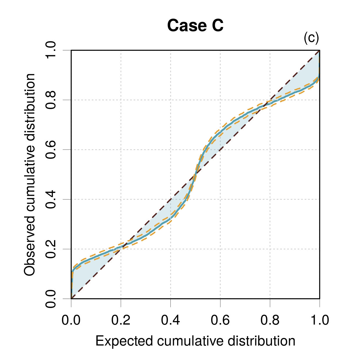
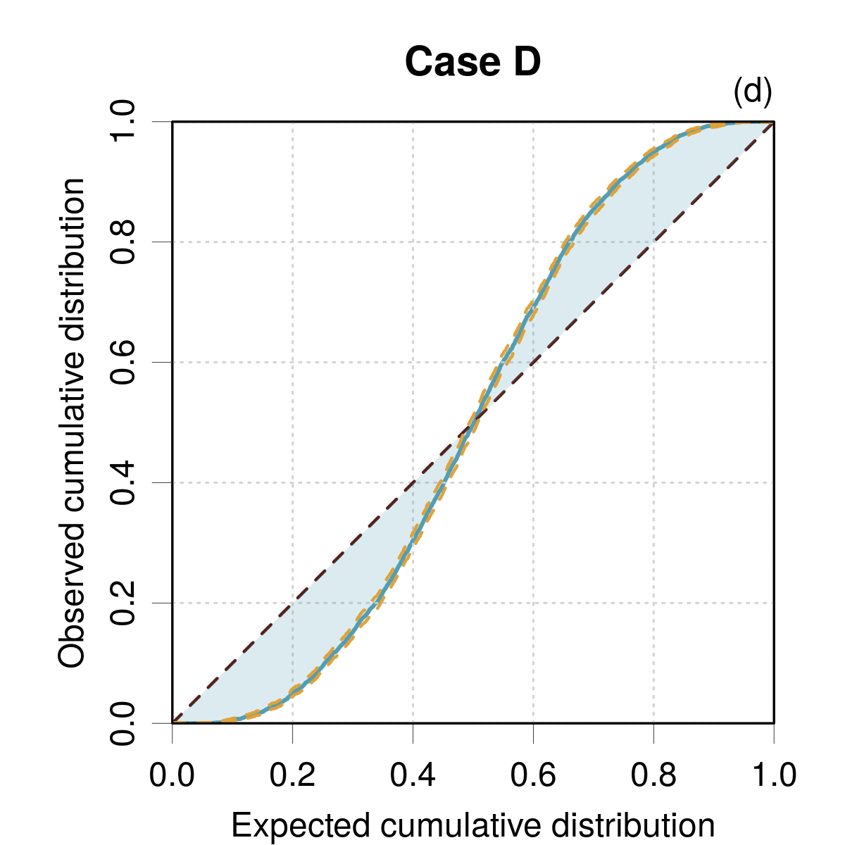
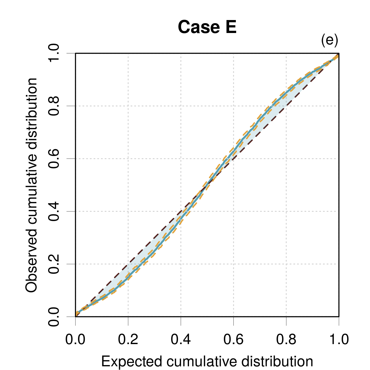
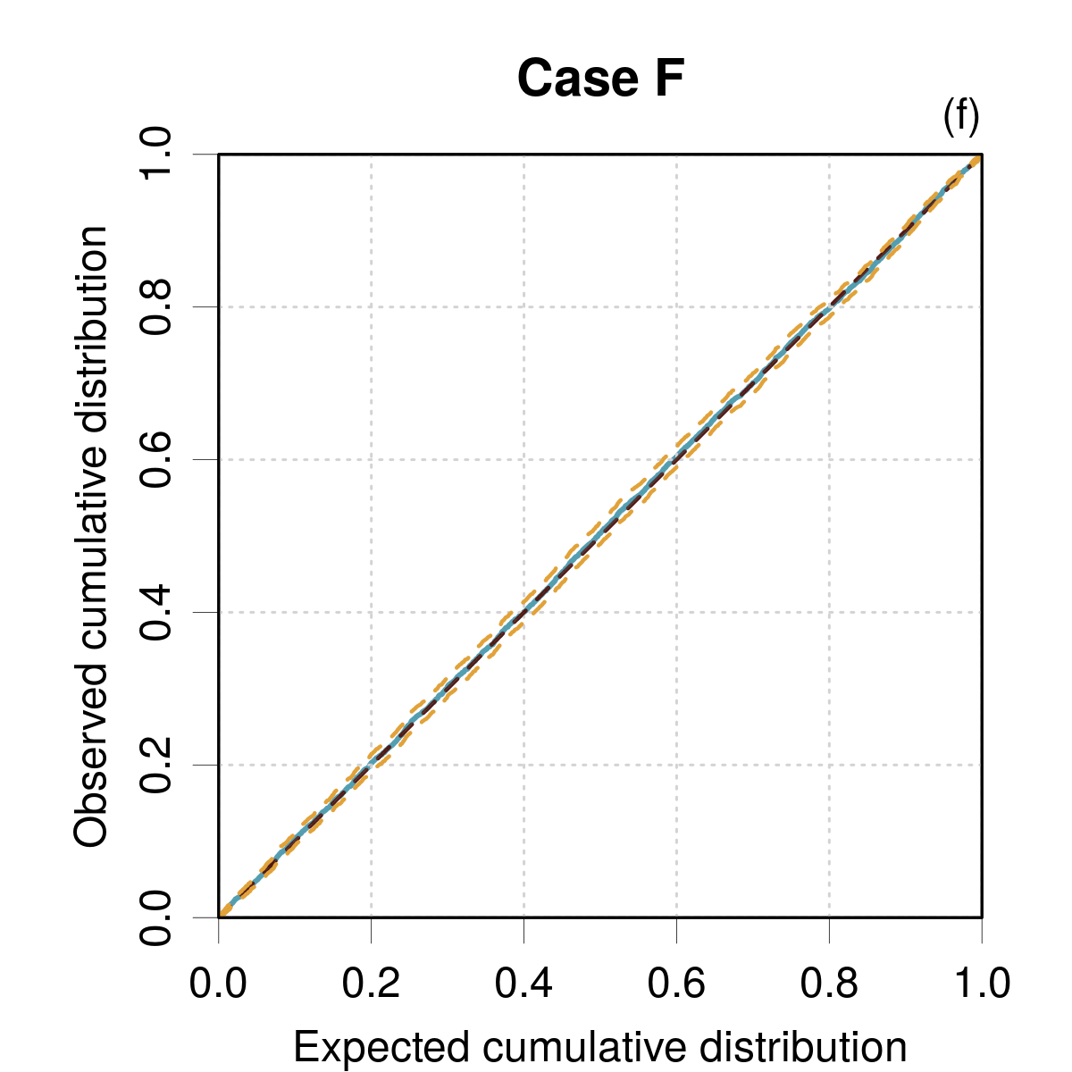
Figure 1: Calibration curves for cases A-F. The calibration curve is a solid blue line. The reference line and its 95 % confidence interval are shown as dashed lines. The shaded area represents the calibration error (miscalibration area).

III.2.1 Calibration curve

In a calibration curve(Kuleshov2018, ), one estimates the probability of errors $E$ to fall within a series of intervals with coverage probability varying in $[0,1]$, and one plots the resulting probability against the target one (Eq. 7). Calibration curves are applicable to homoscedastic datasets.

The method is also referred to as confidence- or intervals-based calibration(Scalia2020, ; Pernot2022a, ; Pernot2022b, ) and formalized as a variant of Eqns. 8-10

$$\lim_{M\rightarrow\infty}\eta_{p,M}=p,\,\forall p\in[0,1]$$ (16)

where

$$\eta_{p,M}=\frac{1}{M}\sum_{i=1}^{M}\boldsymbol{1}\left(E_{i}<q_{p,i}\right)$$ (17)

and $q_{p,i}$ is the quantile for probability $p$ at point $i$.

The ideal calibration curve is the identity line (Fig. 1, Cases A and F). For validation, a 95 % confidence interval is plotted(Pernot2022a, ), either around the empirical curve or the identity line (the latter is preferred when multiple curves are drawn for the conditional case presented later).

As the synthetic datasets provide only a variance-based UQ metric ($u_{E})$, the quantiles in Eq. 17 are calculated by assuming a normal generative distribution, as usually done in the literature. In such cases, deviations from the identity line are not straightforward to interpret, as they might have their origin in the non-consistency of uncertainties (Cases B and C), their non-calibration (Case D) or a bad choice of reference distribution (Case E).

It is interesting to contrast these results with the statistics for average calibration obtained above (Table 2). Case E has satisfying calibration statistics, but presents a slightly problematic calibration curve. This is due to the inadequate choice of a normal generative distribution for this dataset based on a Student’s distribution.

Also, Cases B and C present notably deviant calibration curves despite the fact that they have at least one correct calibration metric. The calibration curve obviously contains more information than the average calibration metrics, but it does not provide direct information on consistency or adaptivity. For instance, without additional information, it is difficult to differentiate the diagnostics for Cases B and D. For variance-based metrics, its use requires also an hypothesis on the generative distribution to estimate the theoretical quantiles, which complicates the interpretation of deviant curves.

III.3 Testing consistency

The validation literature for variance- or interval-based UQ metrics has mostly focused on consistency tests, and several methods are available, which are not fully equivalent. The aim of this section is to highlight the main features of these methods.

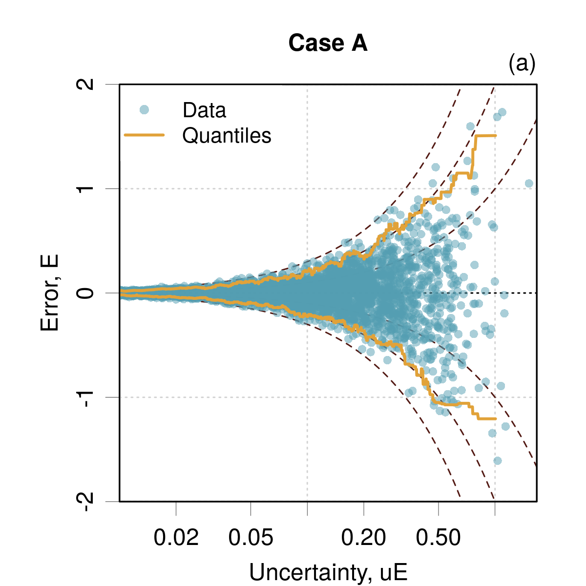
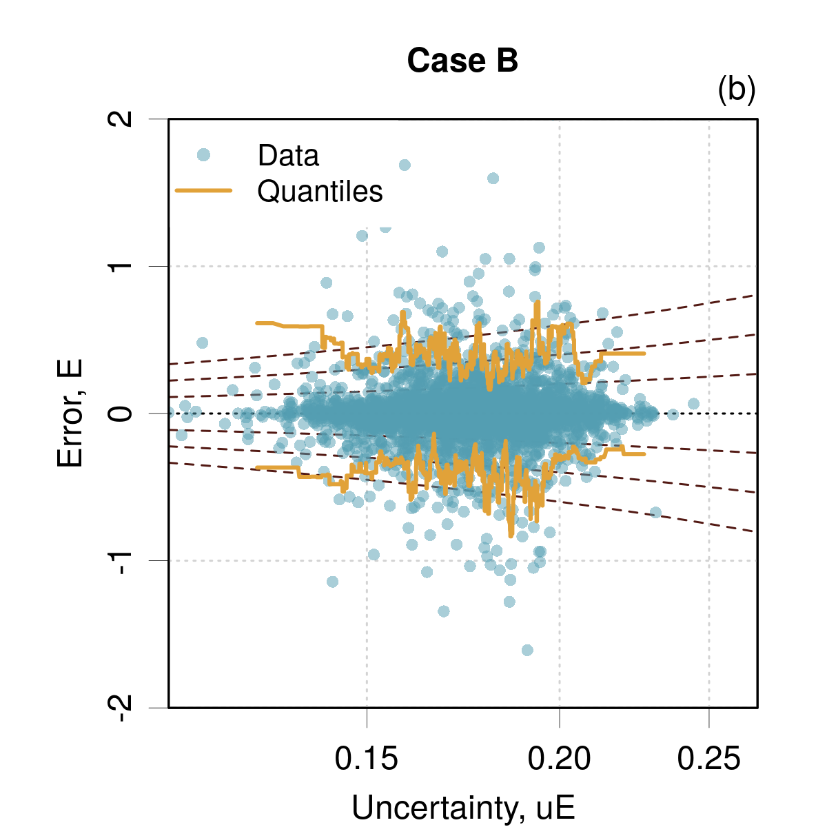
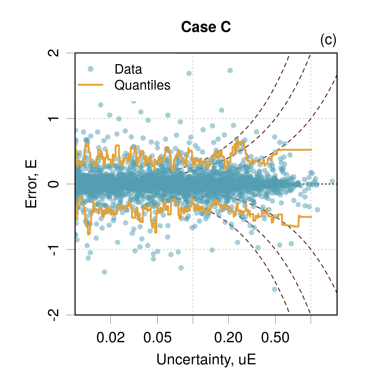
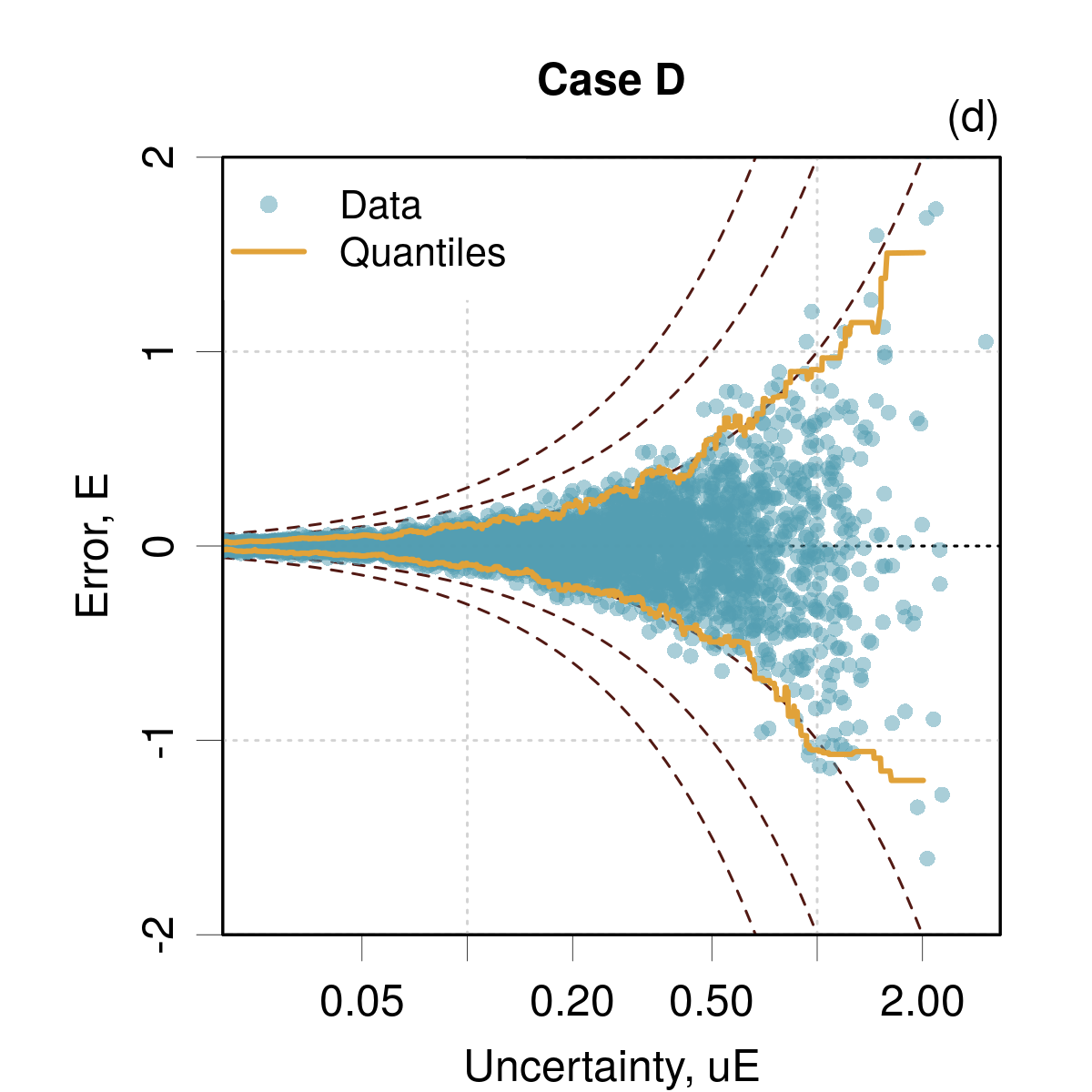
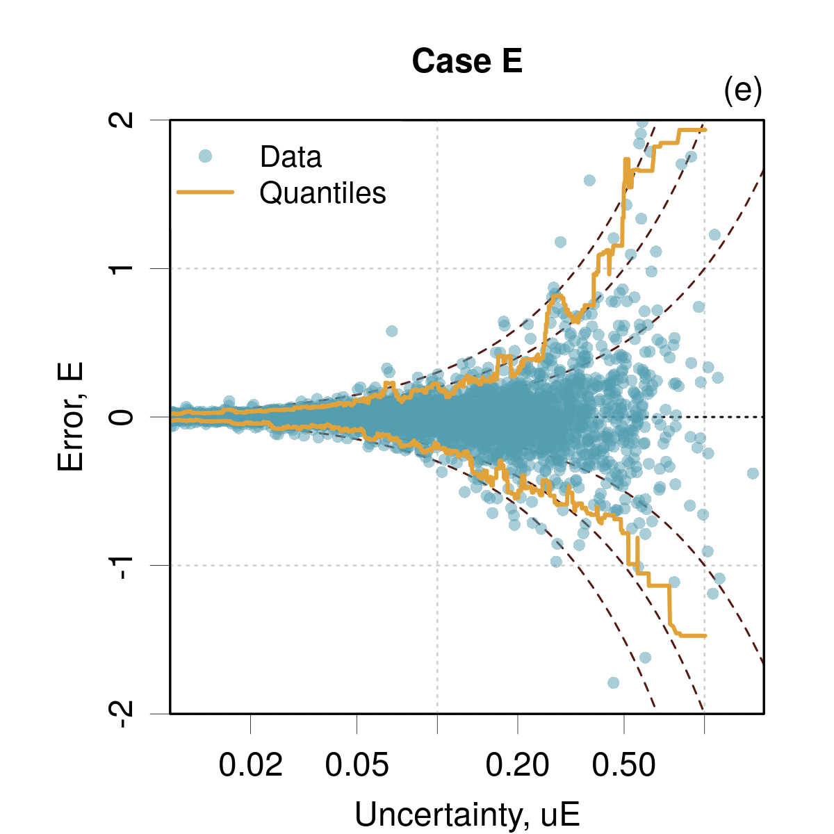
Figure 2: ”$E$ vs $u_{E}$” validation plots for cases A-E. The dashed lines correspond to the $y=\pm kx$ guidelines with $k=1,2,3$. The orange lines represent moving quantiles for a symmetric 95 % interval of the data. They are expected to be parallel and close to the $y=\pm 2x$ lines.

III.3.1 “Error vs. uncertainty” plots

Plotting the errors vs. the uncertainties can be very informative, notably for datasets missing consistency (Janet2019, ; Pernot2022b, ; Hu2022, ). Additional plotting of guiding lines and running quantiles is a welcomed complement to facilitate the diagnostic.(Pernot2022b, ) This is obviously not applicable to homoscedastic datasets.

Examples for the synthetic datasets are shown in Fig. 2. The expected “correct behavior” is to have the running quantile lines for a 95% confidence interval to lie in the vicinity of and parallel to the $E=\pm 2\times u_{E}$ lines. Although the generative distribution is not necessarily normal, one does not expect very large deviations from $k=2$, as seen for instance for the Student’s distribution of Case E. Moreover, the cloud of points should be symmetrical around $E=0$ (absence of bias).

The plots enable to sort out Cases B, C and D without ambiguity. For Cases B and C, the running quantiles are more or less horizontal, indicating an absence of link between the dispersion of $E$ and $u_{E}$. For Case D, the running quantiles follow closely the $k=1$ lines, pointing to a probable overestimation of uncertainties.

For cases where consistency cannot be frankly rejected on the basis of the shape or scale of the data cloud, it is imperative to perform more quantitative tests as presented below. One should not conclude on good consistency simply based on this kind of plot.

III.3.2 Conditional calibration curves in uncertainty space

It is formally possible to construct conditional calibration curves, but, to my knowledge, they have not been proposed in the ML-UQ literature.

Examples are given in Fig. 3 using $u_{E}$ as the conditioning variable with 15 equal-counts bins. In the ideal case (Case A), all the conditional curves lie within the confidence interval estimated for a sample size corresponding to a single bin. Case B shows that the anomaly observed on the average calibration curve is identical at all uncertainty levels, pointing to a consistency problem or a wrong choice of generative distribution. Case C is interesting, as it shows that the small oscillations of the average calibration curve around the identity line are attenuated compared to the much larger deviations observed for conditional curves. This points to the fact that a seemingly good calibration curve might hide a non-consistent case. The large dispersion of conditional curves is less likely to be due to a poor choice of generative distribution (unless the generative distribution varies strongly with $u_{E}$) and points to a lack of consistency. Cases D and E offer the same diagnostic as for case B, with an ambiguity between non-consistency and generative distribution problem. Using a Student’s-$t_{\nu=4}$ generative distribution for Case E solves the problem [Fig. 3(f)].

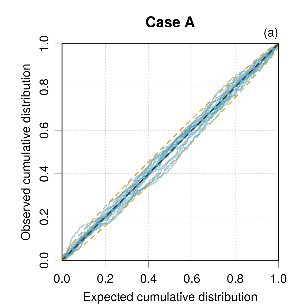
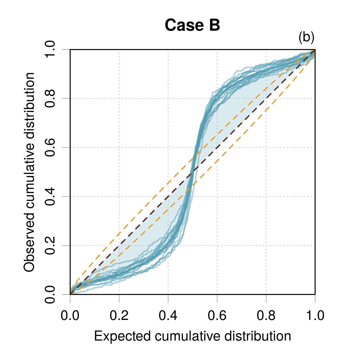
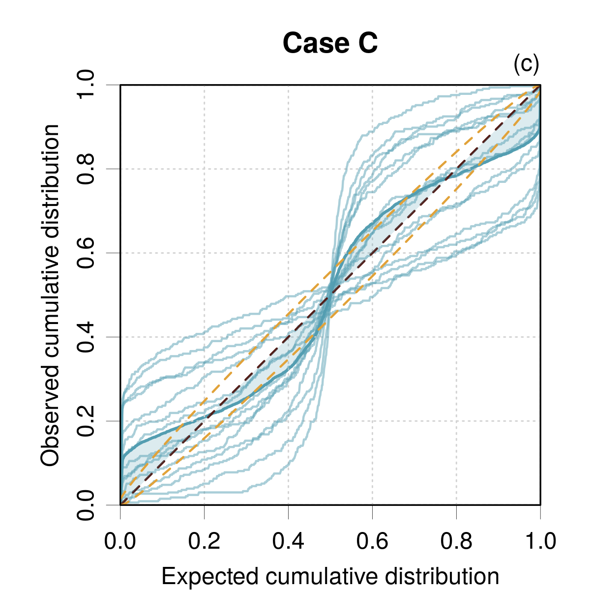
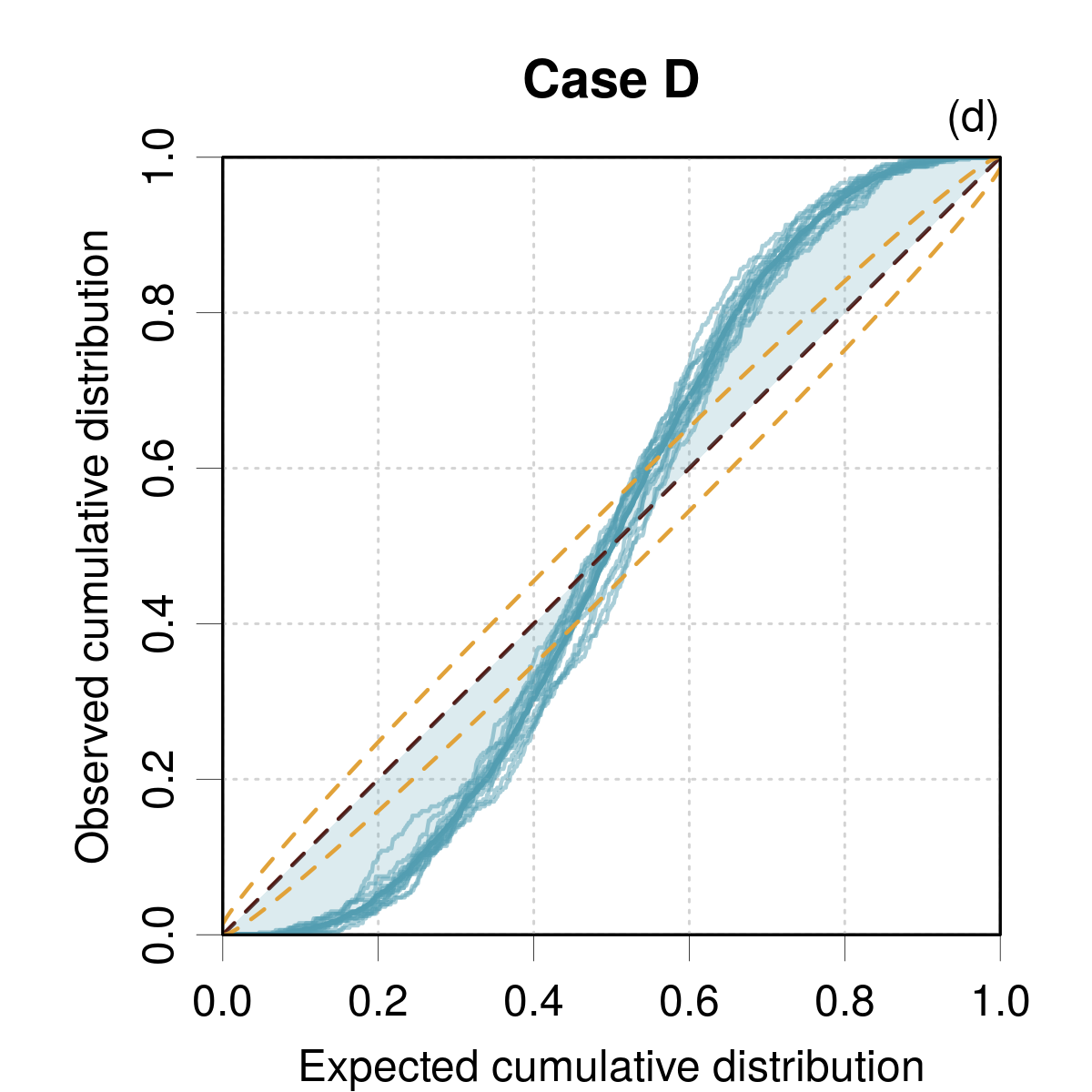
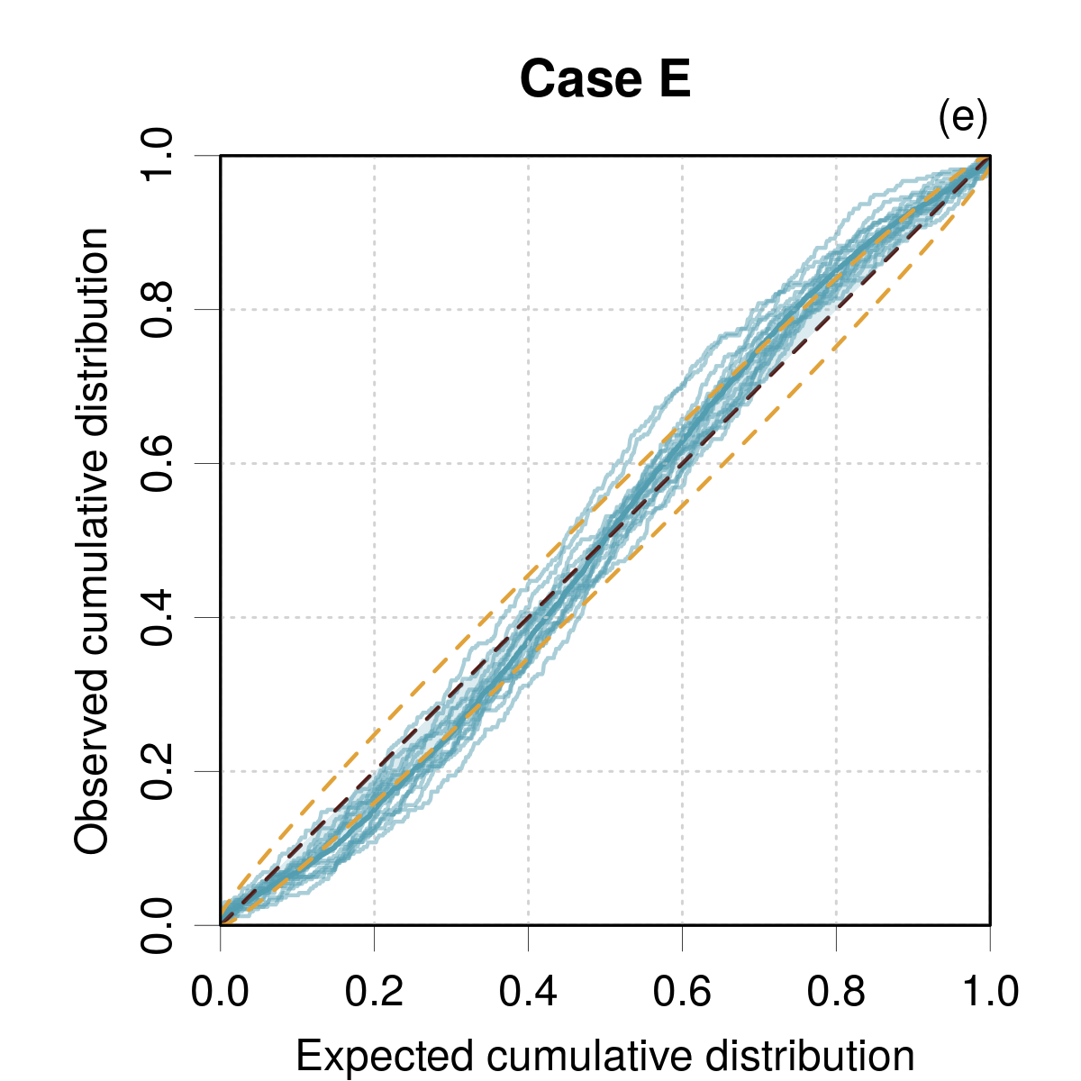
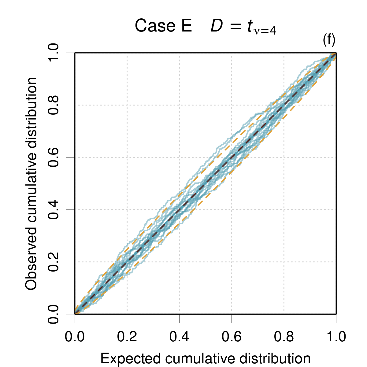
Figure 3: Conditional calibration curves vs $u_{E}$ for cases A-E. The average calibration curve is a thick blue line, the conditional curves are thin blue lines. The reference line and its 95 % confidence interval are dashed orange lines. The dataset has been split according to the binning of $u_{E}$ into 15 equal-counts sets.

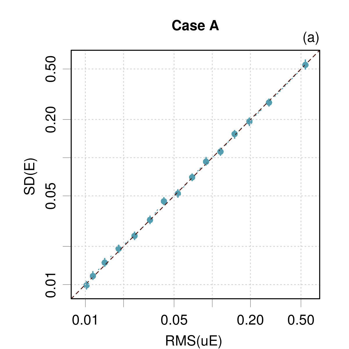
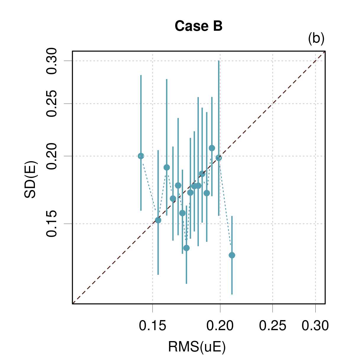
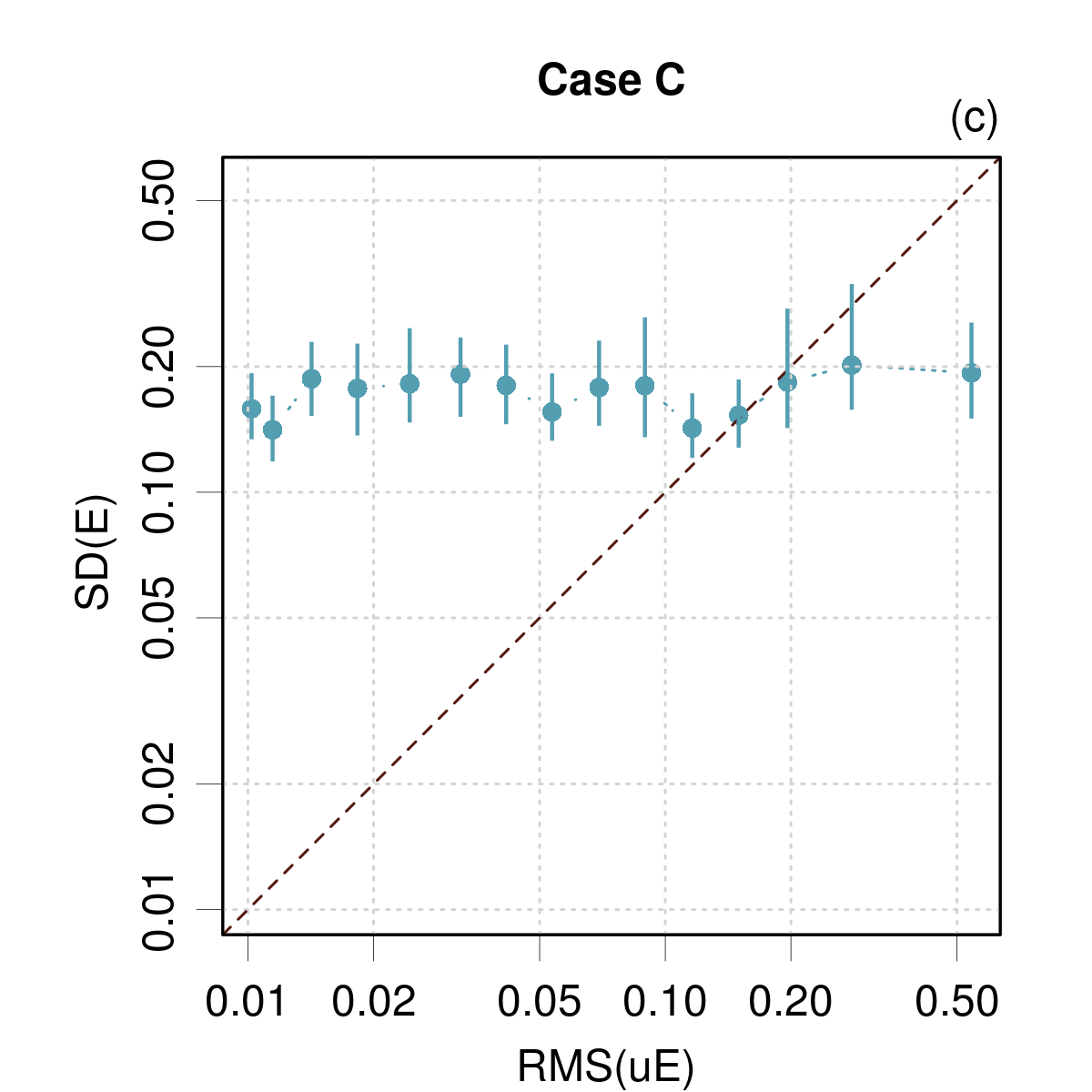
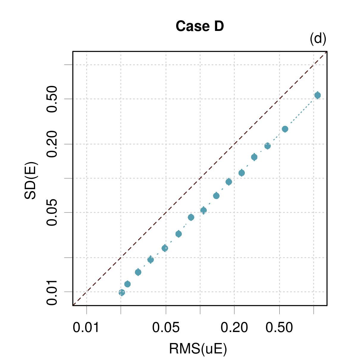
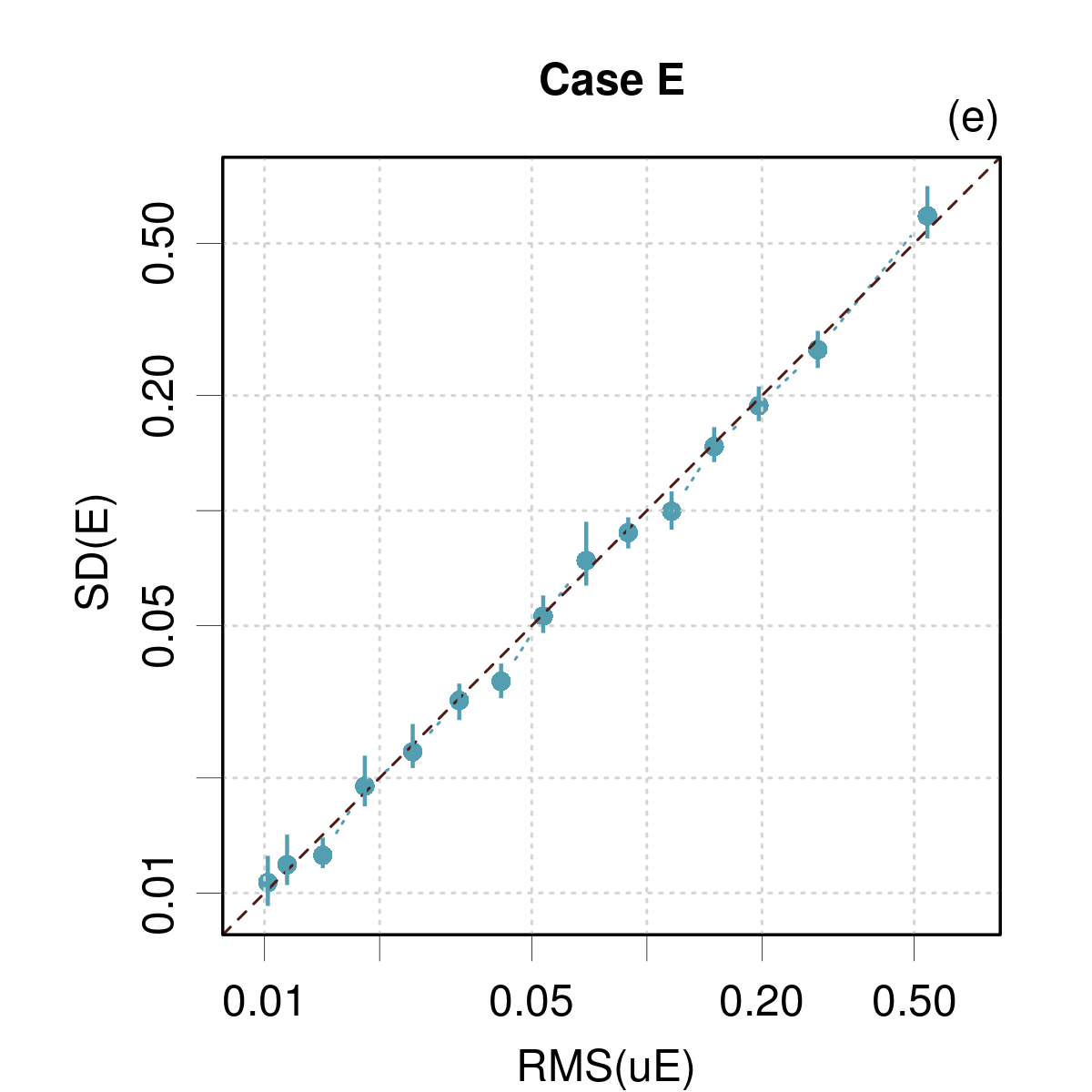
Figure 4: Reliability diagrams for cases A-E. Not applicable to case F (homoscedastic).

III.3.3 Reliability diagram

So-called reliability diagrams(Guo2017, ; Levi2020, ) test consistency through Eq. 5 over data subsets, where the data are ordered by increasing $u_{E}$ values and split into bins. This method is therefore not usable for homoscedastic datasets. Reliability diagrams can also be found in the literature as error-based calibration plots(Scalia2020, ) (not to be confounded with calibration curves, Sect. III.2.1), RvE plots(Palmer2022, ), or RMSE vs. RMV curves(Vazquez-Salazar2022, ).

For convenience, the square roots of the terms of Eq. 5 are used, linking the mean uncertainty in each bin (as the root mean squared (RMS) of $u_{E}$, also called root mean variance (RMV)) with the RMSE or RMSD of $E$ (both are equivalent for unbiased errors).

For consistent datasets, the reliability curve should lie close to the identity line, up to statistical fluctuations due to finite bin counts. For a conclusive analysis of deviations from the identity line, the amplitude of these finite size effects should be estimated, for instance by bootstrapping.(Pernot2022b, )

The binning strategy is important(Nixon2019, ): some authors advocate for bins with identical counts,(Levi2020, ; Scalia2020, ) other for bins with identical widths(Palmer2022, ). Both choices are defensible according to the distribution of uncertainties, notably the absence or presence of heavy tails. It should also be noted that the insensitivity of Eq. 2 to the pairing between $E$ and $u_{E}$ might still be a hindrance for large bins, but its effect should decrease when the bins get smaller. However, small bins are affected by large statistical fluctuations. The binning strategy should thus be designed to offer a good compromise. An adaptive binning scheme mixing both strategies is proposed in Appendix B.

For the synthetic datasets, I use a default choice of 15 equal-counts bins, leading to about 333 points per bin (Fig. 4). The non-consistent cases (B, C, D) are correctly identified, although for case B the deviation from the identity line is not noticeable except for the two extreme bins.

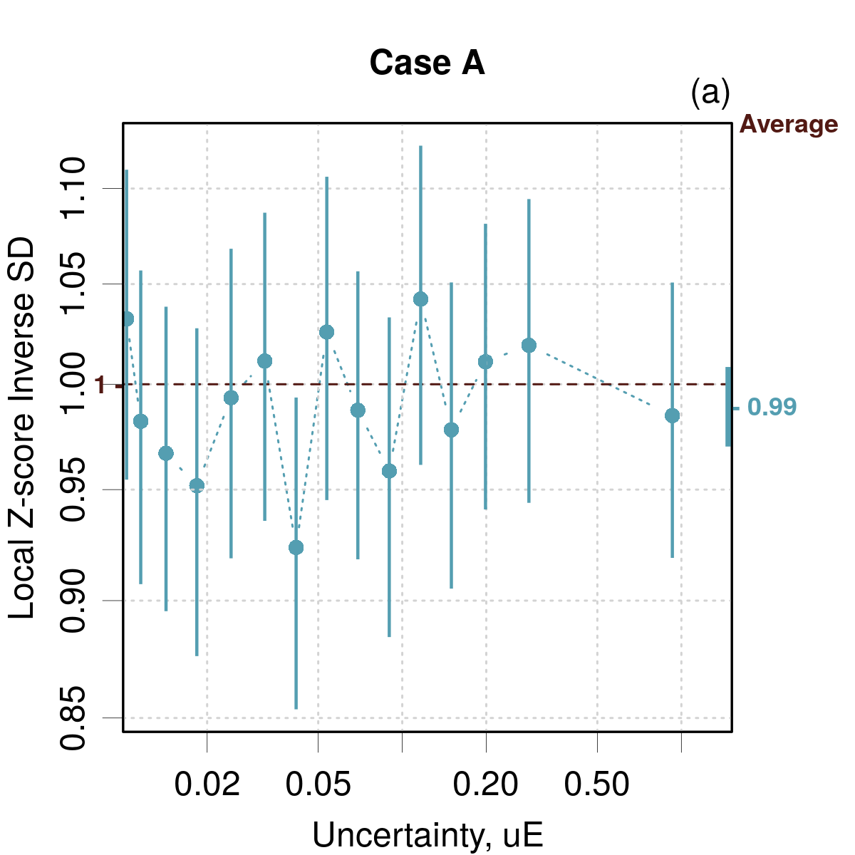
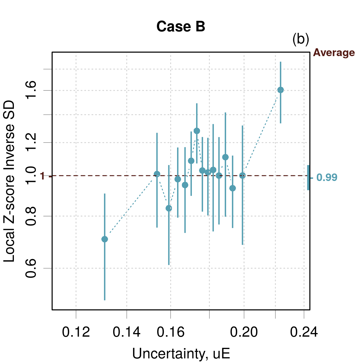
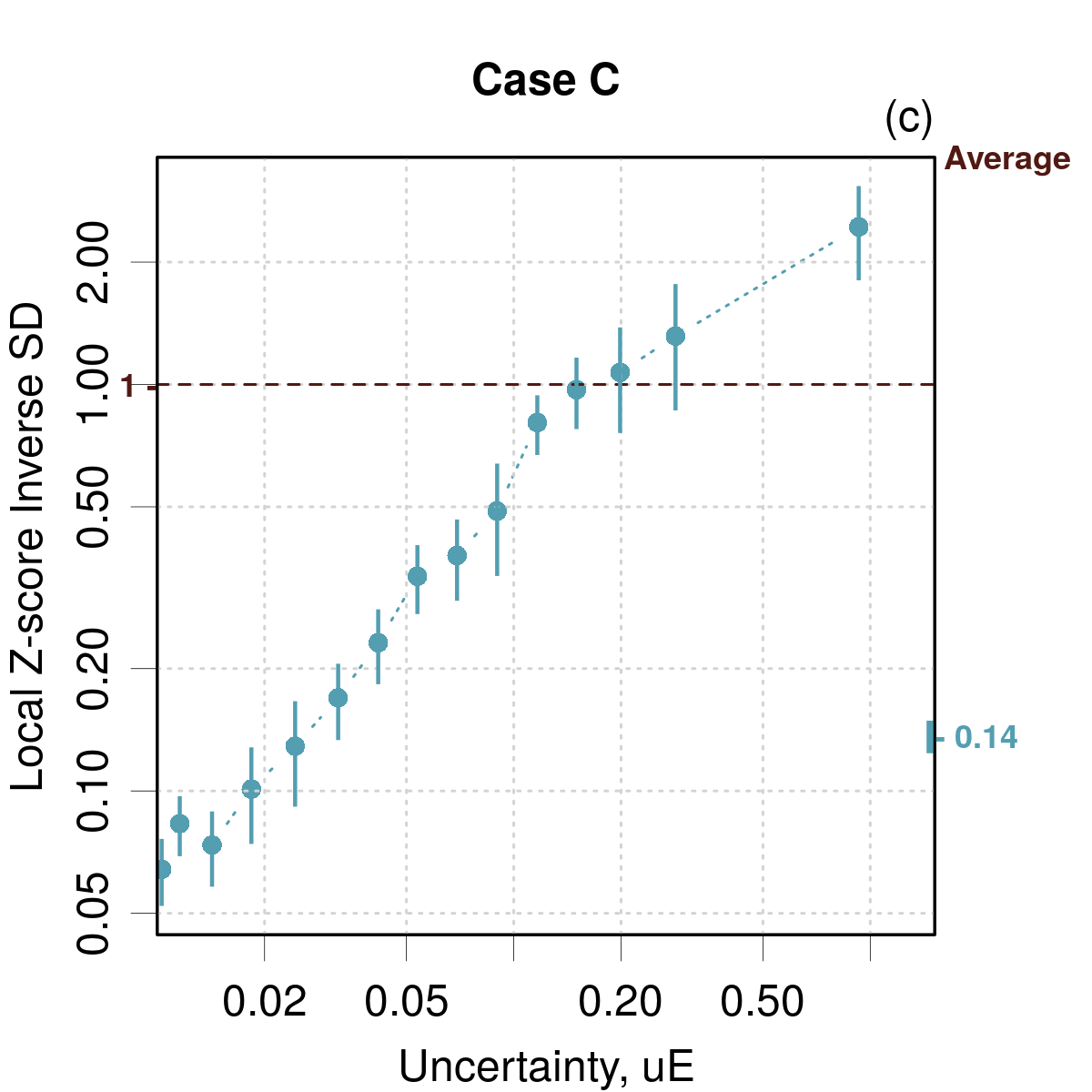
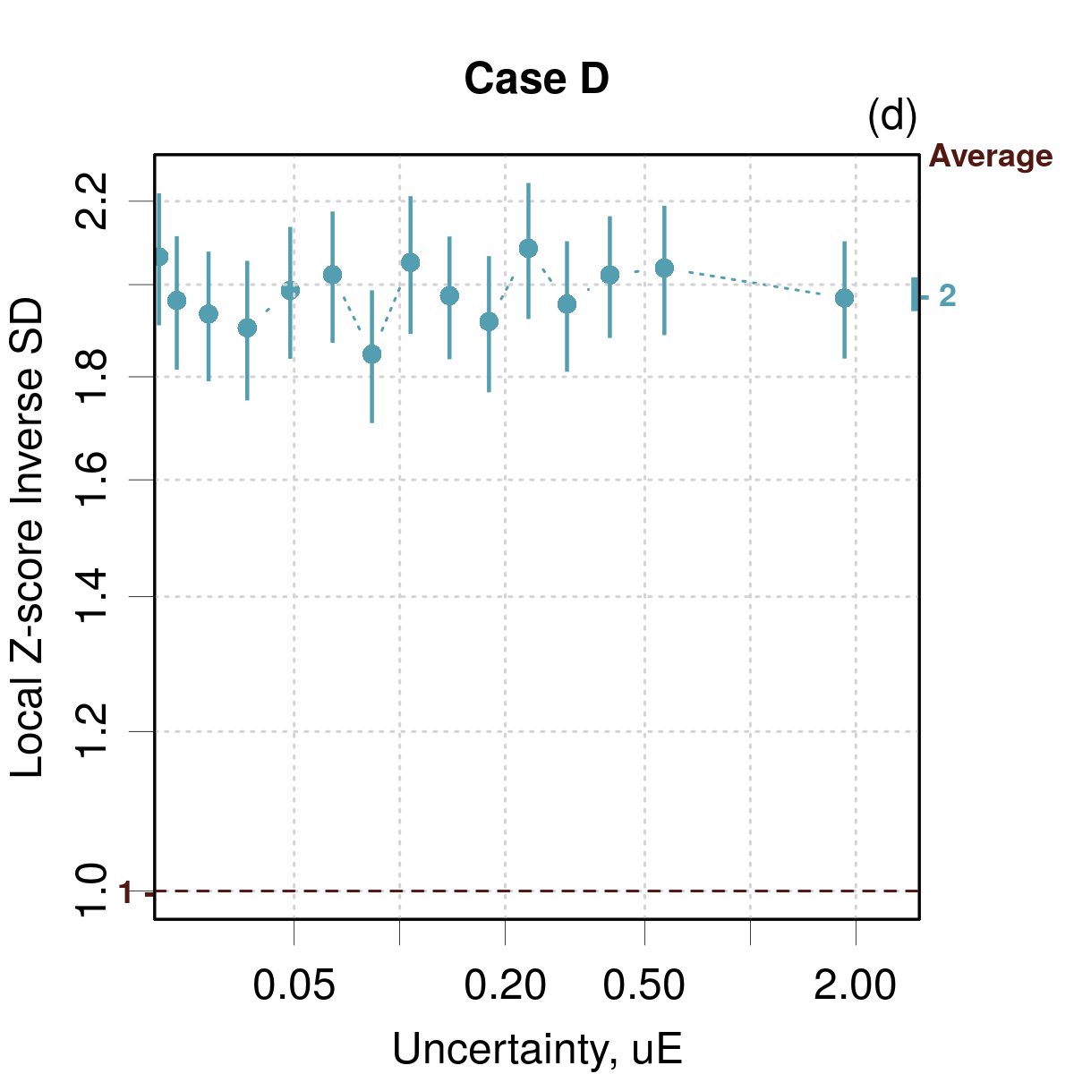
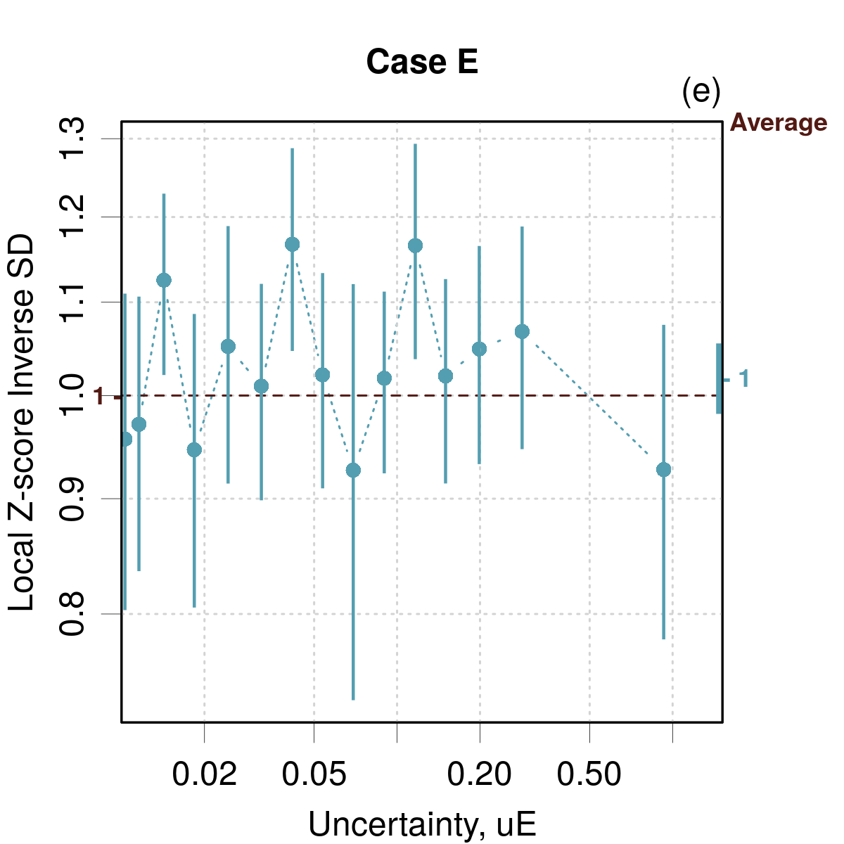
Figure 5: LZISD analysis for cases A-E. Not applicable to case F (homoscedastic). The points are reported at the center of the bins. The error bars correspond to 95 % confidence intervals on the statistic. The value and error bar reported on the right axis corresponds to the statistic for the full dataset (Average).

III.3.4 Local Z-Variance analysis in uncertainty space

LZV analysis was introduced by Pernot(Pernot2022a, ) as a method to test local calibration based on Eq. 6. As for reliability diagrams, it is based on a binning of the data according to increasing uncertainties. For each bin, one estimates $\mathrm{Var}(Z)$ and compares it to 1. Here again, error bars on the statistic should be provided to account for finite bin counts.(Pernot2022a, )

Assuming a nearly constant uncertainty value within a bin, values of $\mathrm{Var}(Z)$ smaller/larger than 1 indicate over-/under-estimated uncertainties (by a factor $\sqrt{\mathrm{Var}(Z)}$). This suggests an alternative plot of the inverse of the standard deviation of $Z$, $\mathrm{Var}(Z)^{-1/2}$, instead of $\mathrm{Var}(Z)$, which provides a more direct reading and quantification of the local uncertainty deviation. This Local Z-scores Inverse Standard Deviation (LZISD) analysis is used throughout this study.

Application of the LZISD analysis to the synthetic datasets confirms the diagnostics of non-tightness for cases B, C and D (Fig. 5). For Case B, the deviation from the reference is more legible than on the corresponding reliability diagram [Fig. 4(b)], and the largest local deviations can be directly quantified to about 30 % in default and 60 % in excess (these extreme values are probably underestimated, as they result from a bin averaging).

III.3.5 Local Coverage Probability analysis in uncertainty space

Conditional coverage with respect to an uncertainty metric is available through the Local Coverage Probability analysis.(Pernot2022a, ) It can be directly built from prediction intervals if available, or estimated from prediction uncertainties and an hypothetical generative distribution. In both cases, the empirical coverages are drawn for a series of data subsets based on the binning of the conditioning variable and for the available target probabilities. The LCP analysis of consistency is not applicable to homoscedastic datasets.

For the synthetic datasets (Fig. 6), one makes the hypothesis of a normal generative distribution to build prediction intervals from the uncertainties for $\mathcal{P}=\{25,50,75,95\}$. Case A presents perfect conditional coverages over the full uncertainty range and probability levels. For Case B, the empirical coverages are too large, except at the $P=95$ % level. The dependency along $u_{E}$ is weak, except for the two extreme intervals, as was observed on the LZISD analysis. A contrario, Case C presents a strong coverage variation across $u_{E}$, with inadequate mean PICP values. For Case D, the overestimated uncertainties produce intervals with excessive coverage, uniformly across the uncertainty range. Finally, Case E suffers again from the misidentification of the generative distribution, which is solved by using the correct distribution to generate the intervals [Fig. 6(f)].

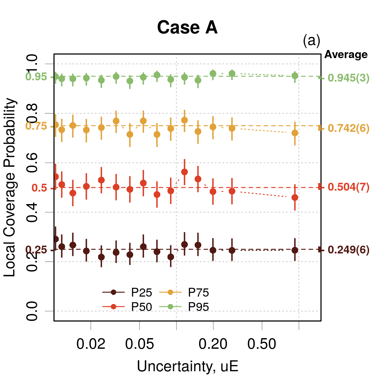
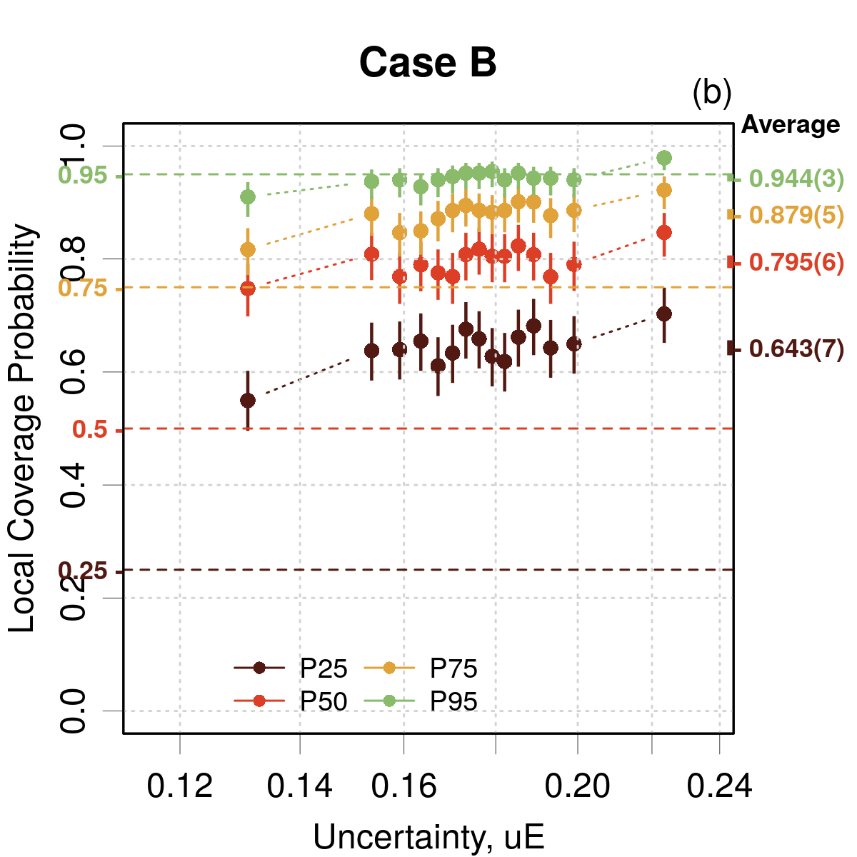
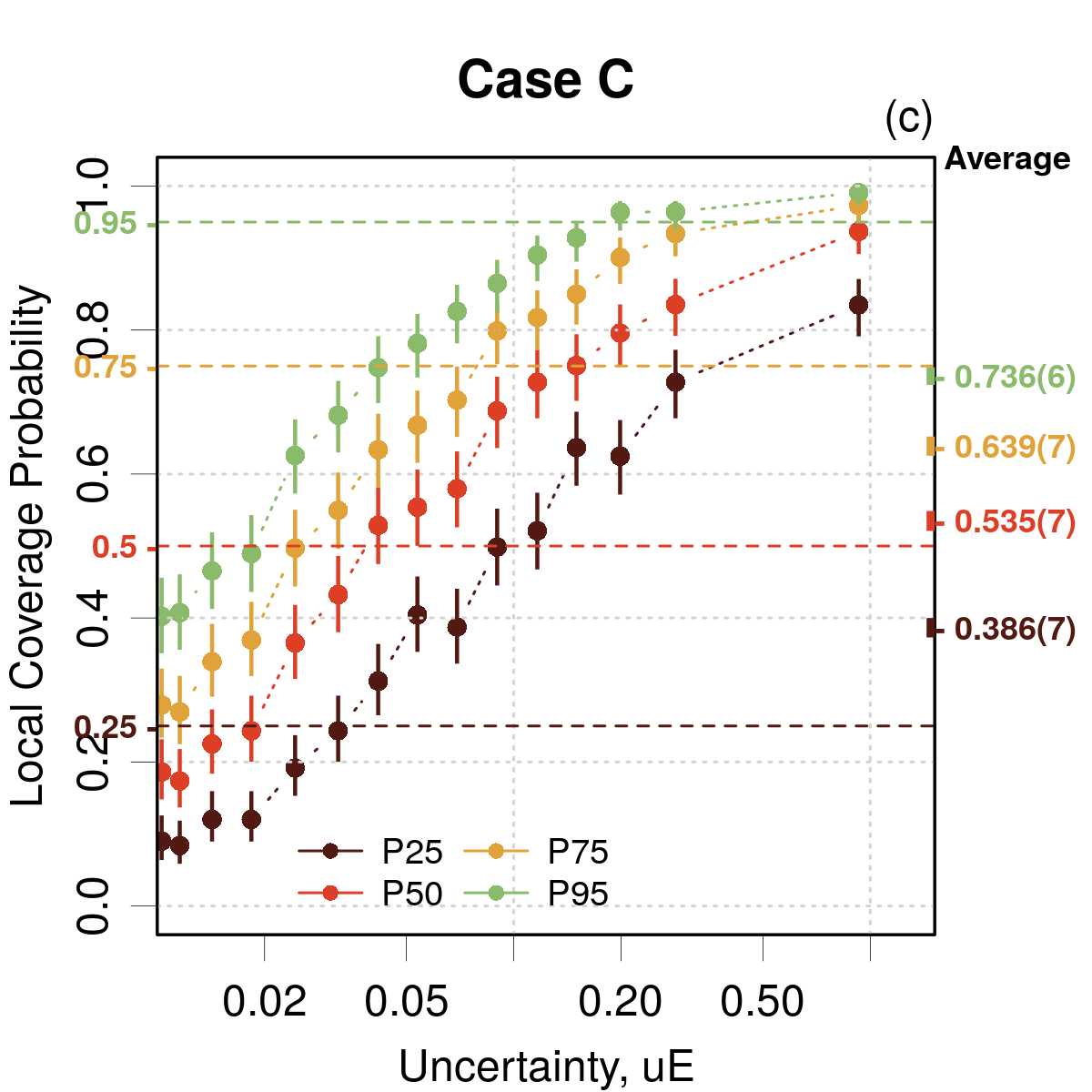
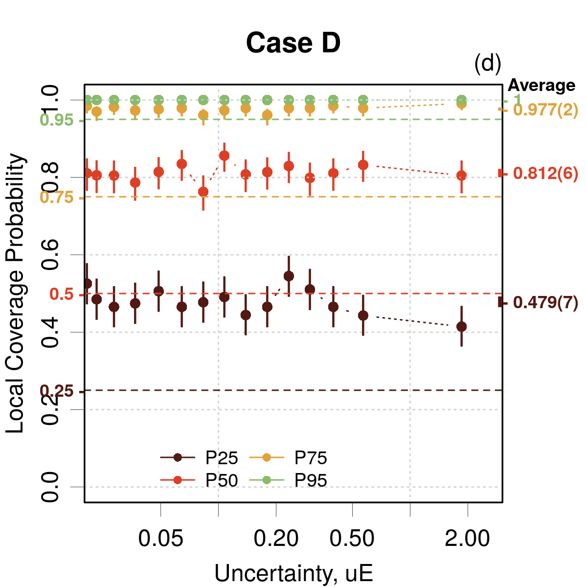
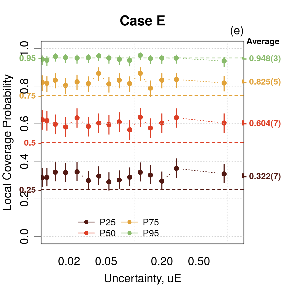
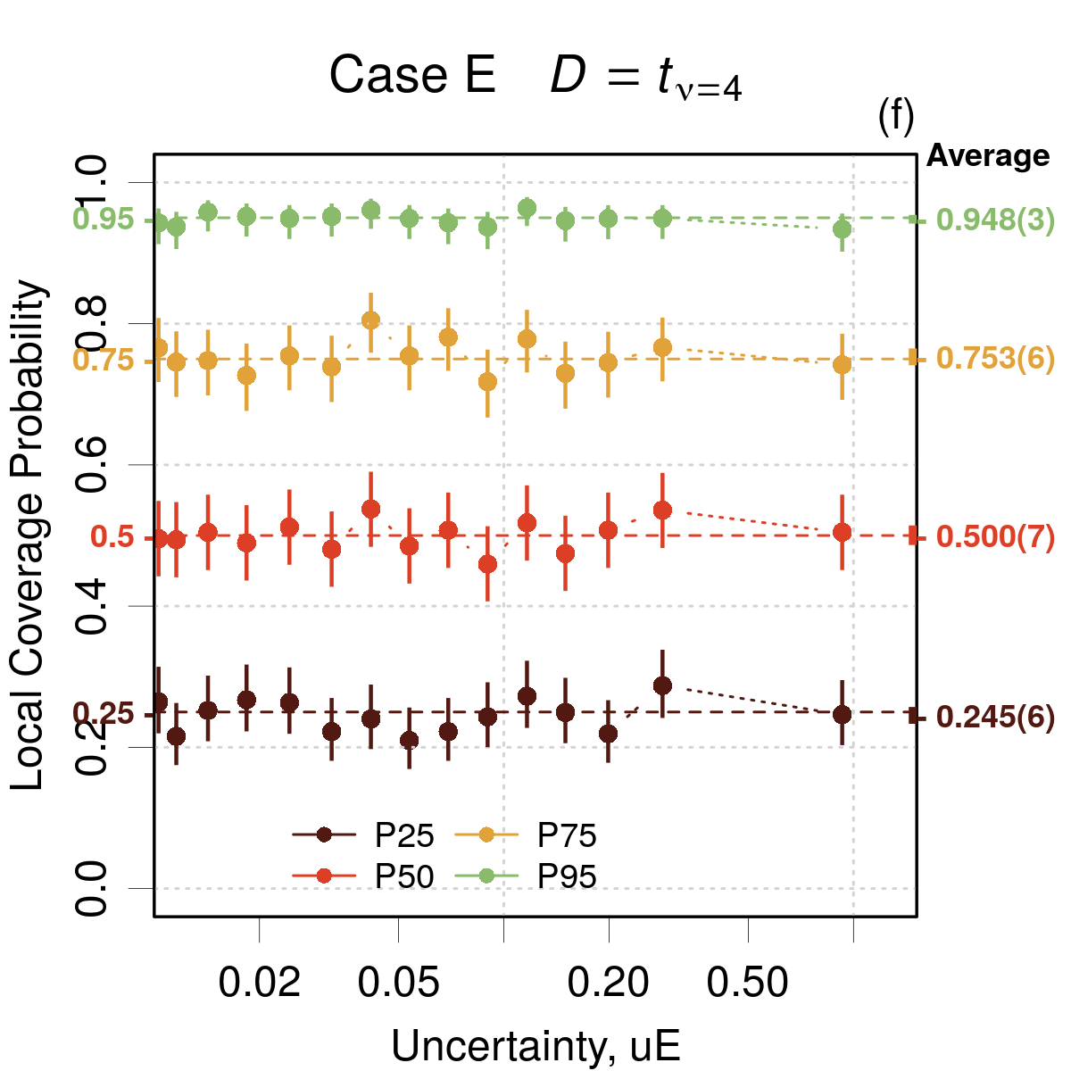
Figure 6: LCP analysis conditional to $u_{E}$ for cases A-E. Not applicable to case F (homoscedastic). The points are reported at the center of the bins. The error bars correspond to 95 % confidence intervals on the statistic. The value and error bar reported on the right axis corresponds to the statistic for the full dataset (average coverage).

When a PICP value reaches 1.0, one gets no information about the mismatch amplitude with the target probability. The Local Ranges Ratio analysis (LRR) has been proposed by Pernot(Pernot2022b, ) to solve this problem. It estimates the ratio between the width of the empirical interval and the width of the theoretical interval. This tool is not exploited in the present study, but its availability should be kept in mind,

III.3.6 Confidence curve

A confidence curve is established by estimating an error statistic $S$ on subsets of $C$ iteratively pruned from the points with the largest uncertainties.(Scalia2020, ) Technically, it is a ranking-based method, as (1) it is insensitive to the scale of the uncertainties, and (2) the relative ranking of the errors and uncertainties plays a determinant role. It is not applicable to homoscedastic datasets.

If one defines $u_{k}$ as the largest uncertainty left after removing the $k$ % largest uncertainties from $u_{E}$ ($k\in\{0,1,\ldots,99\}$), a confidence statistic is defined by

$$c_{S}(k;E,u_{E})=S\left(E\,|\,u_{E}<u_{k}\right)$$ (18)

where $S$ is an error statistic – typically the Mean Absolute Error (MAE) or Root Mean Squared Error (RMSE) – and $S\left(E\,|\,u_{E}<u_{k}\right)$ denotes that only those errors $E_{i}$ paired with uncertainties $u_{E_{i}}$ smaller than $u_{k}$ are selected to compute $S$. A confidence curve is obtained by plotting $c_{S}$ against $k$. Both normalized and non-normalized confidence curves are used in the literature, but the RMSE-based non-normalized version should be preferred for the validation of variance-based UQ metrics.(Pernot2022c, )

A monotonously decreasing confidence curve reveals a desirable association between the largest errors and the largest uncertainties, an essential feature for active learning. It might also enable to detect unreliable predictions. But, in order to test consistency, one needs to compare $c_{S}$ to a reference.

Reference curves.

As already mentioned, only the order of $u_{E}$ values is used to build a confidence curve, and any change of scale of $u_{E}$ leaves $c_{S}$ unchanged. Without a proper reference, $c_{S}$ cannot inform us on calibration or consistency.

An oracle curve can be generated by reordering $u_{E}$ to match the order of absolute errors. This can be expressed as

$$O(k;E)=c_{s}(k;E,|E|)$$ (19)

It is evident from the above equation that the oracle is independent of $u_{E}$ and therefore useless for calibration testing. Recast in the probabilistic framework introduced above, the oracle would correspond to a very implausible error distribution $D$, such that $E_{i}=\pm u_{E_{i}}$. Although it is offered as the default reference curve in some validation libraries, I strongly recommend against its use for variance- or interval-based UQ metrics.

Using Eq. 1, a probabilistic reference curve $P$ can be generated by sampling pseudo-errors $\widetilde{E}_{i}$ for each uncertainty $u_{E_{i}}$ and calculating a confidence curve for $\left\{\tilde{E},u_{E}\right\}$, i.e.,

$$P(k;u_{E})=\left\langle c_{S}(k;\tilde{E},u_{E})\right\rangle_{\tilde{E}}$$ (20)

where a Monte Carlo average is taken over samples of

$$\widetilde{E}_{i}\sim D(0,u_{E_{i}})$$ (21)

The sampling is repeated to have converged mean and confidence band at the 95 % level, typically 500 times.

In contrast to the oracle, which depends exclusively on the errors, the probabilistic reference depends on $u_{E}$ and a choice of distribution $D$, but it does not depend on the actual errors $E$. Comparison of the data confidence curve to $P$ enables to test if $E$ and $u_{E}$ are correctly linked by the probabilistic model, Eq. 1, i.e. to test consistency. For RMSE-based confidence curves, $P$ does not depend on the choice of generative distribution (only the width of the confidence band does). This is not the case for MAE-based confidence curves, which makes them less suitable.(Pernot2022c, ) Given the choice of a generative distribution $D$, interval-based metrics can be transformed to variance-based metrics and used to build a confidence curve and probabilistic reference.

One can check in Fig. 7 that consistency problems are well identified by the comparison of a confidence curve to the associated probabilistic reference (Cases B-D). When small deviations are observed, it is however difficult to discriminate between a genuine consistency problem and a bad choice of generative distribution for $P$ (Case E). The choice of the appropriate distribution for Case E leaves the confidence and reference curve unchanged, but widens the confidence band of the probabilistic reference, ensuring validation of consistency.

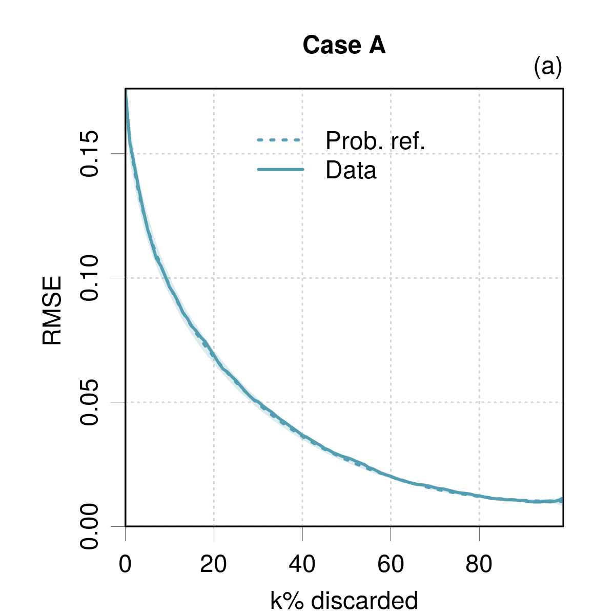
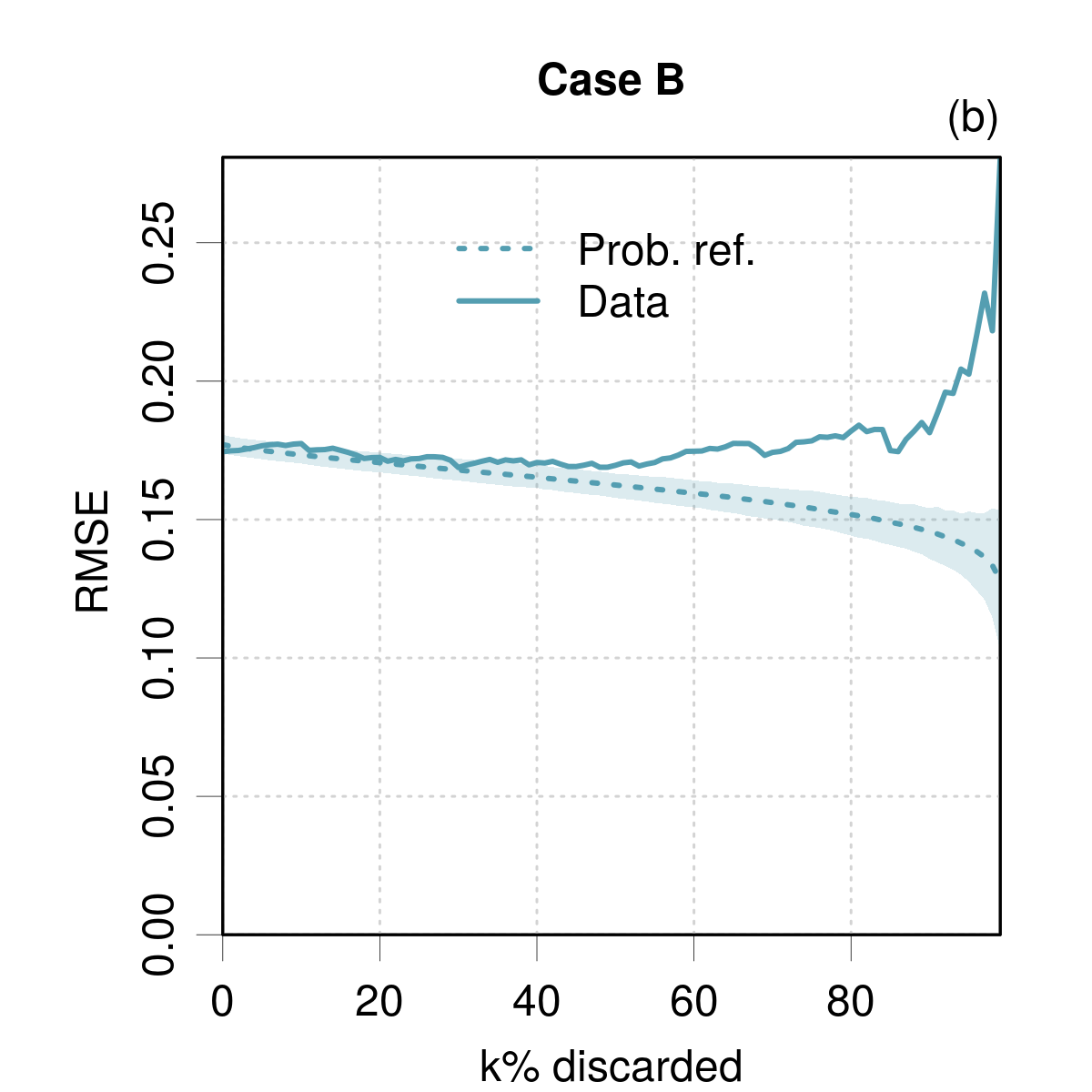
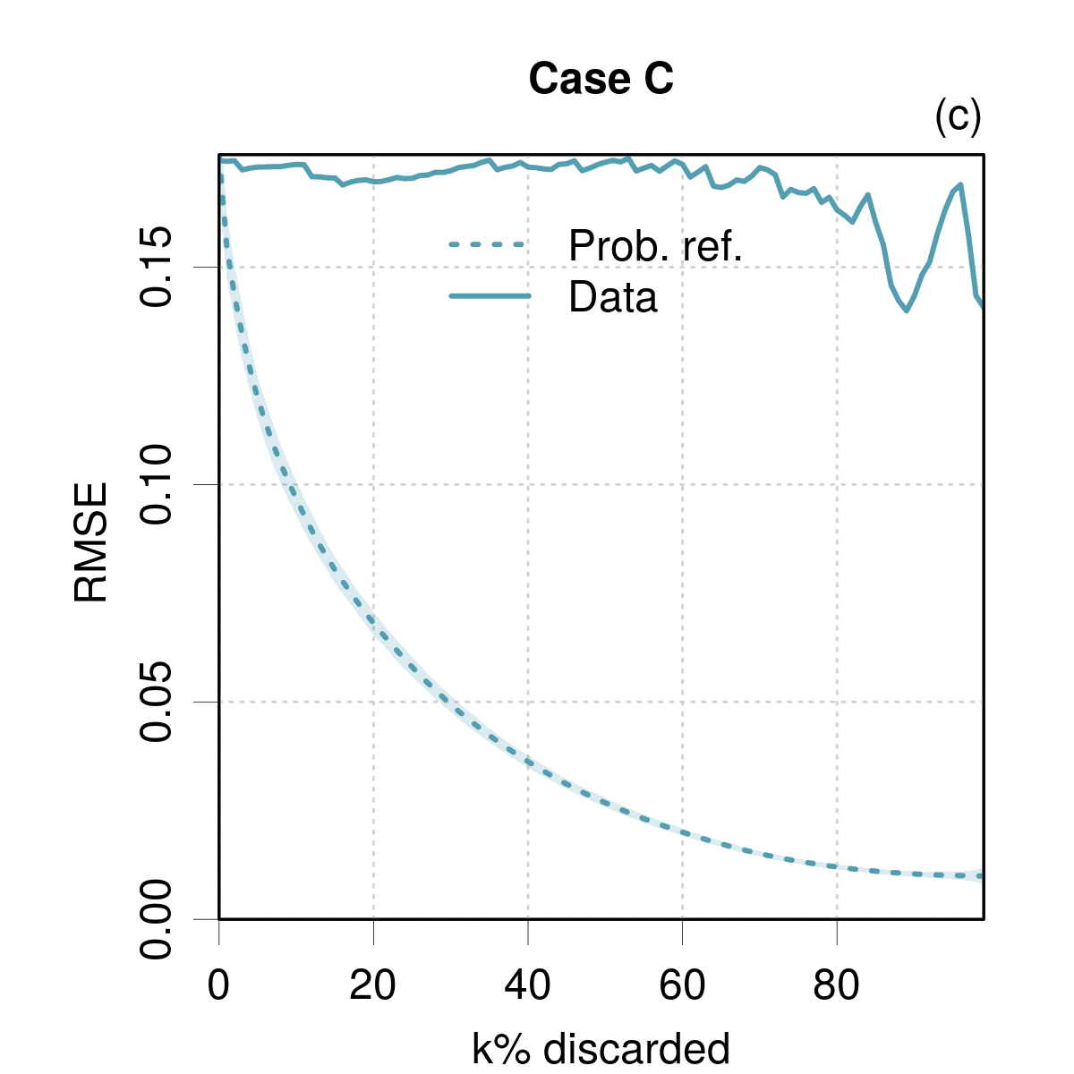
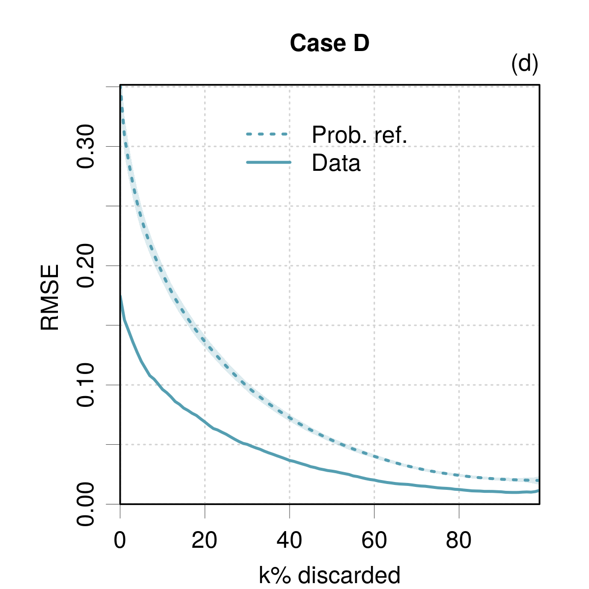
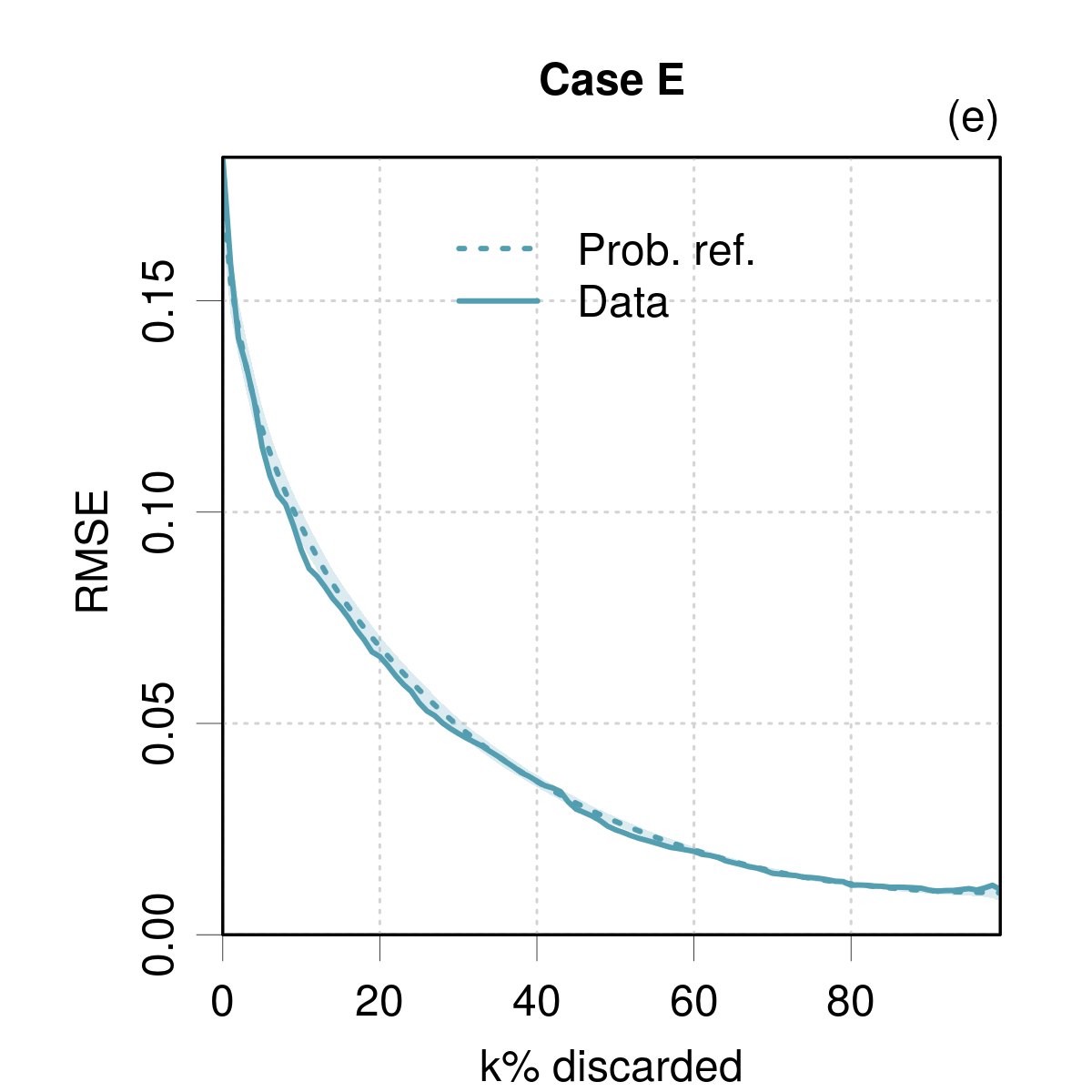
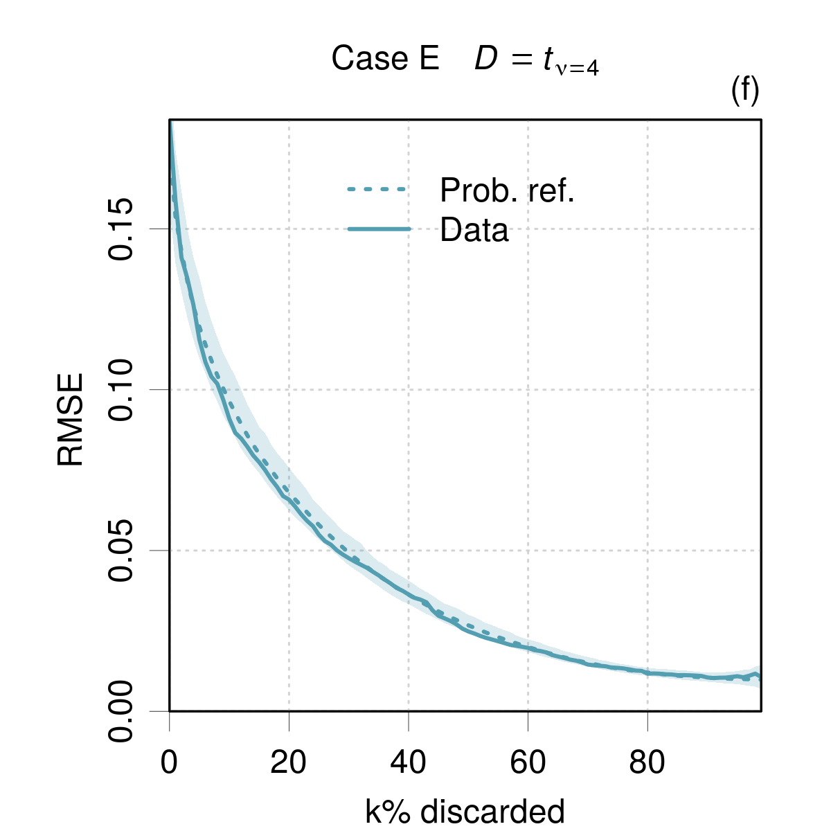
Figure 7: Confidence curves for cases A-E. Not applicable to case F (homoscedastic). The solid blue line is the data confidence curve, the dashed blue line is the probabilistic reference line and the light blue area defines its 95 % confidence interval.

III.4 Testing adaptivity

Adaptivity is not commonly tested in the ML-UQ literature, except maybe through a binary approach discerning in-distribution and out-of-distribution predictions.(Scalia2020, ; Hu2022, )

III.4.1 $Z$ vs Input feature plot

The analog of the “$E$ vs $u_{E}$” plot for consistency is to plot the z-scores $Z$ as a function of a relevant input feature $X$ to check adaptivity. The distribution of $Z$ should be homogeneous along $X$ and symmetric around $Z=0$. Here again, one can use guide lines $Z=\pm 2$ and compare with running quantiles for a 95% confidence interval of $Z$ values.

Conditioning on $X$ is shown in Fig.8 for the synthetic datasets. Considering the shape of the data clouds, adaptivity can be clearly rejected in cases B and C, while the dispersion of the z-scores is insufficient in Case D. Validation of adaptivity in the other cases require a more quantitative approach.

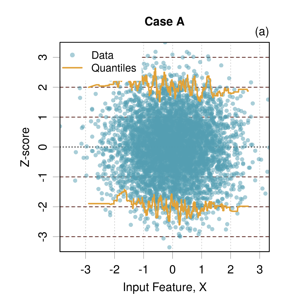
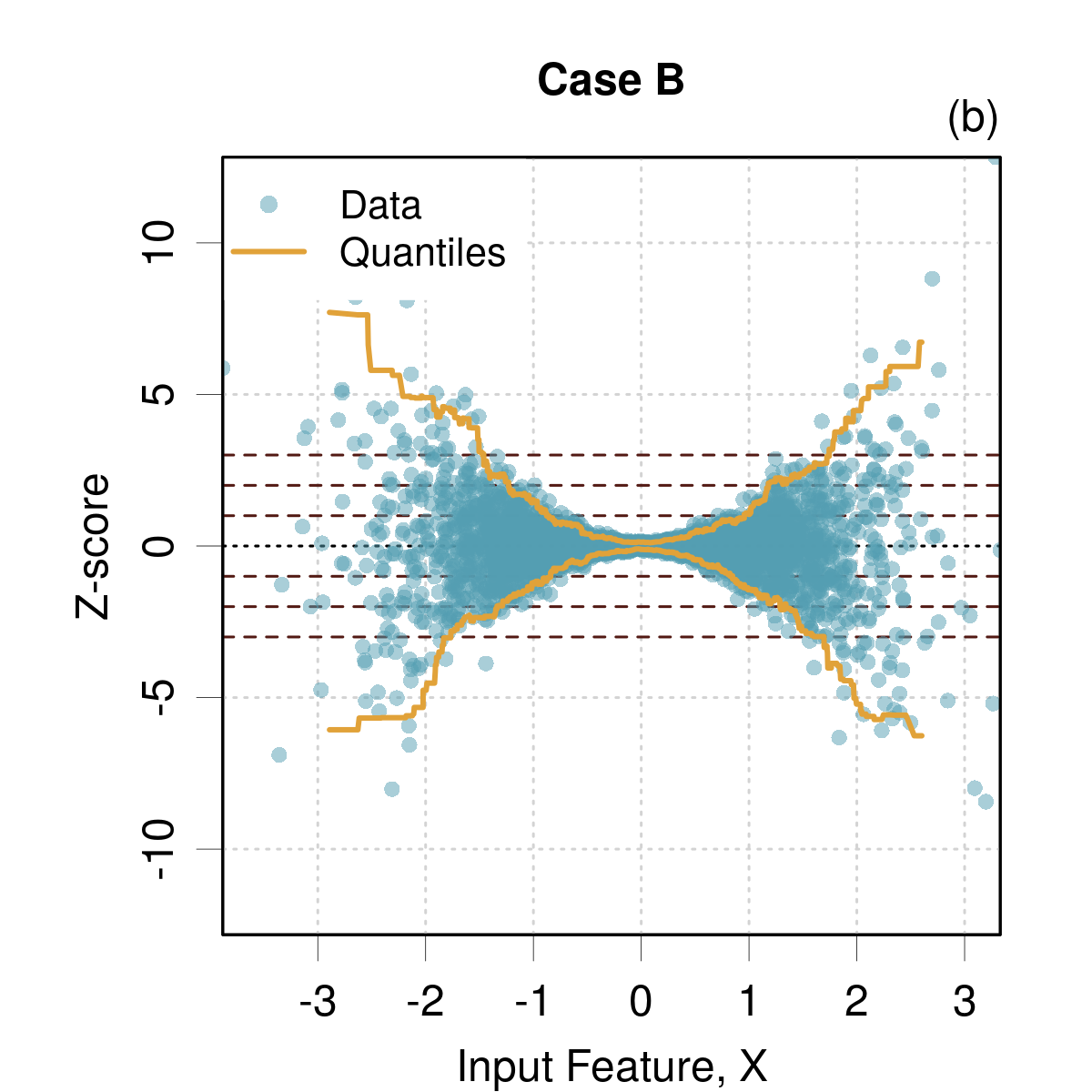
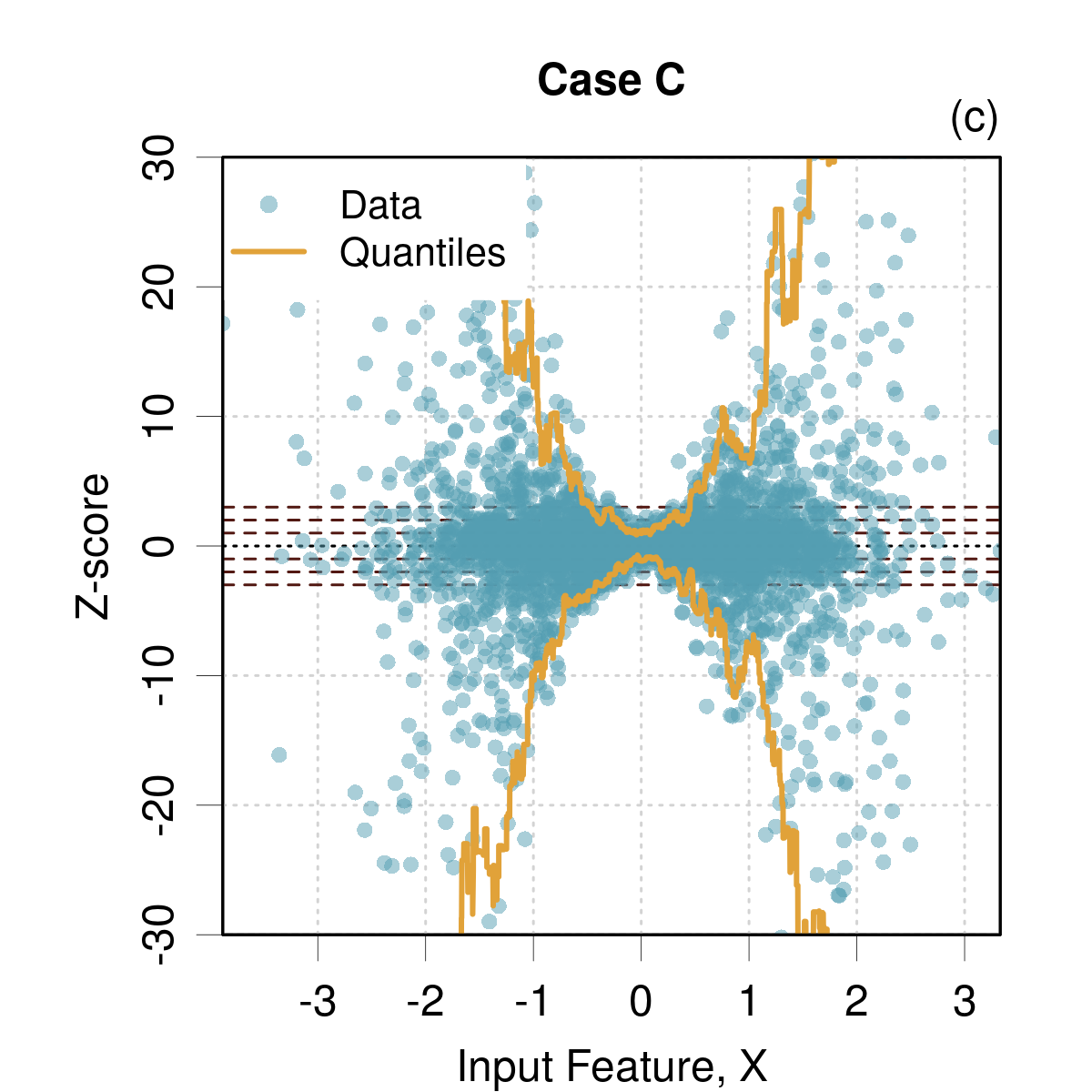
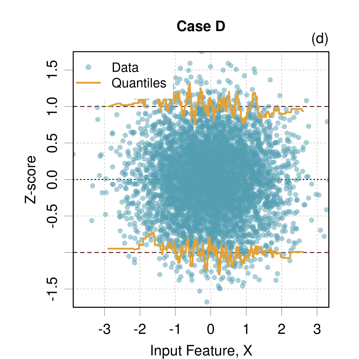
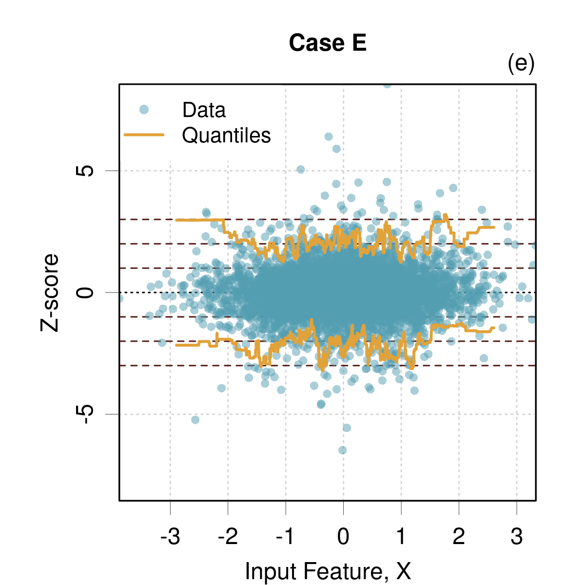
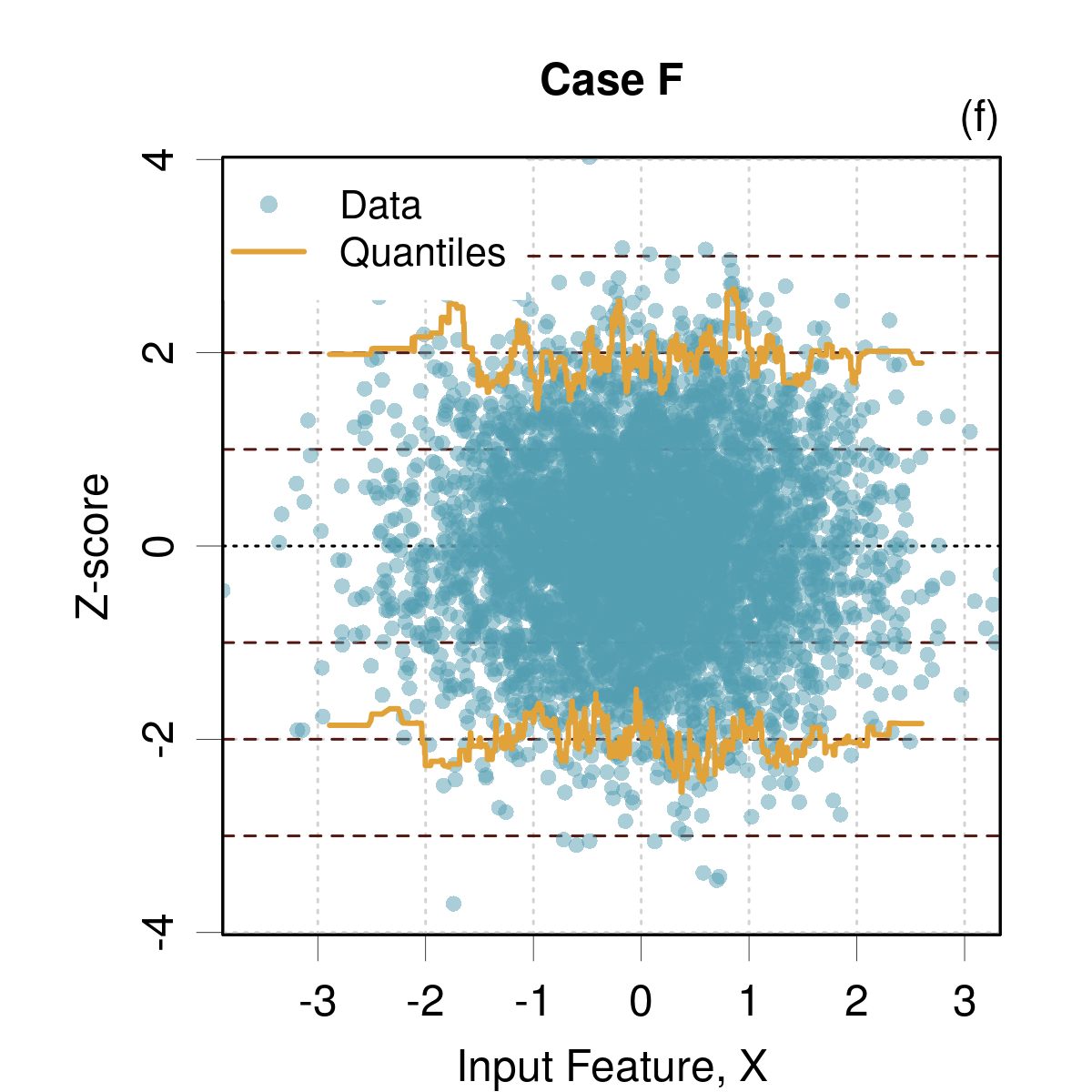
Figure 8: ”$Z$ vs $X$” validation plots for cases A-F.

III.4.2 Conditional calibration curves in input feature space

The same principle as used for consistency testing (Sect. III.3.2) can be applied to adaptivity by grouping the data according to the binning of a relevant input feature $X$. The method can now be applied to homoscedastic datasets.

Application to the synthetic datasets is presented in Fig. 9. For Cases A and F, one would conclude to a good adaptivity along $X$ . For the other cases, the deviations from the identity line are similar to those observed when testing consistency, except for Case B, where the conditional calibration curves are much more dispersed.

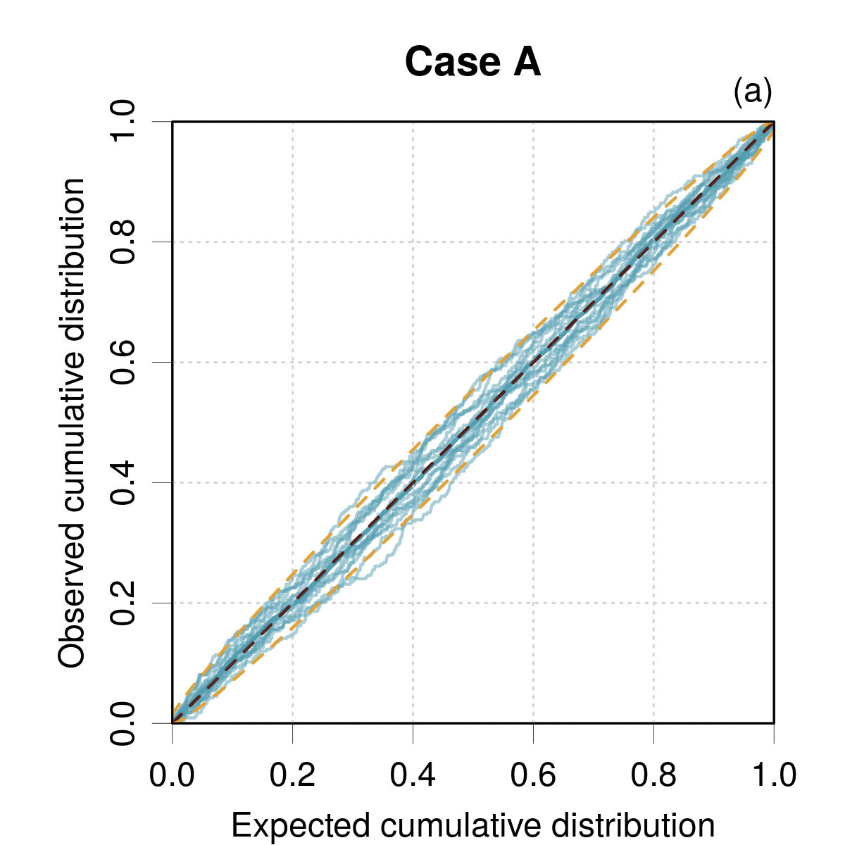
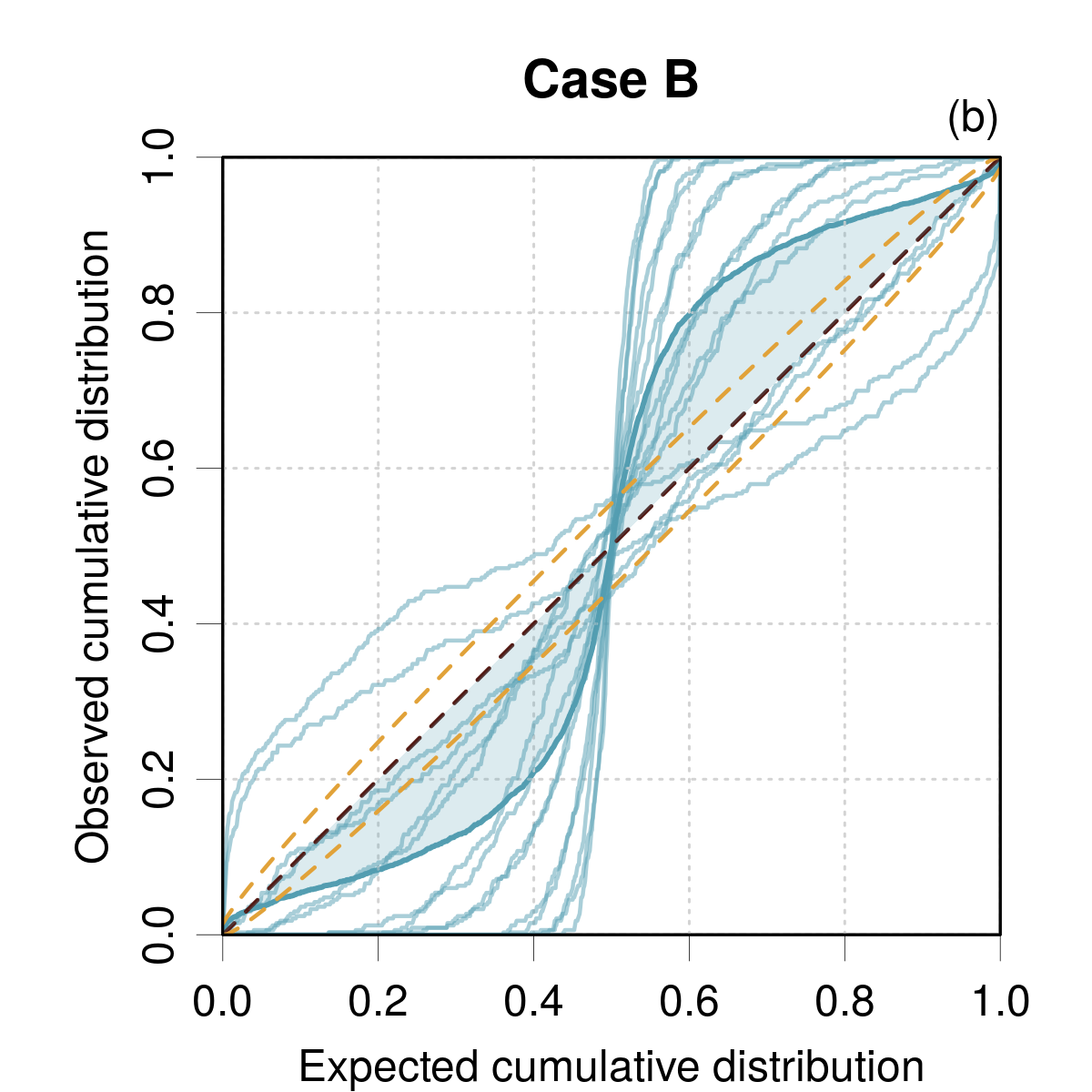
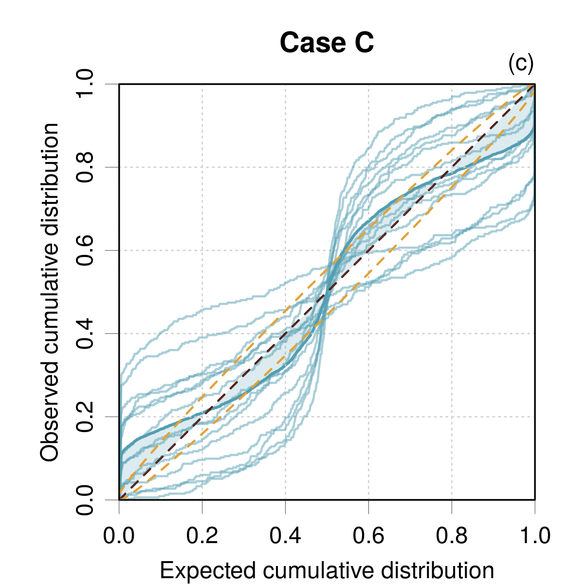
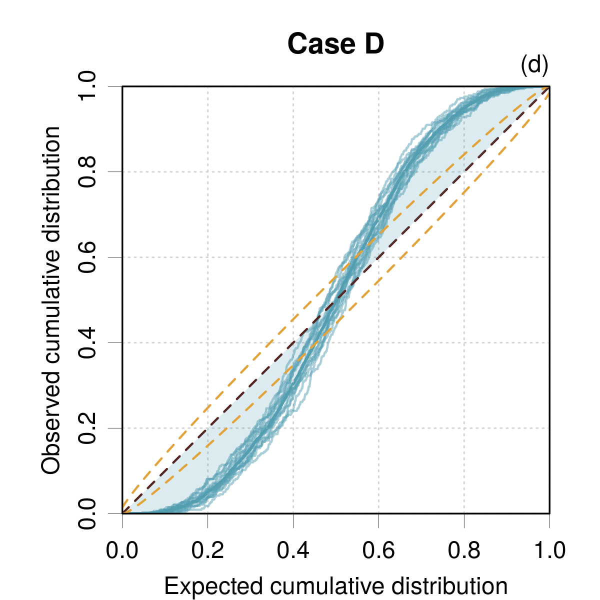
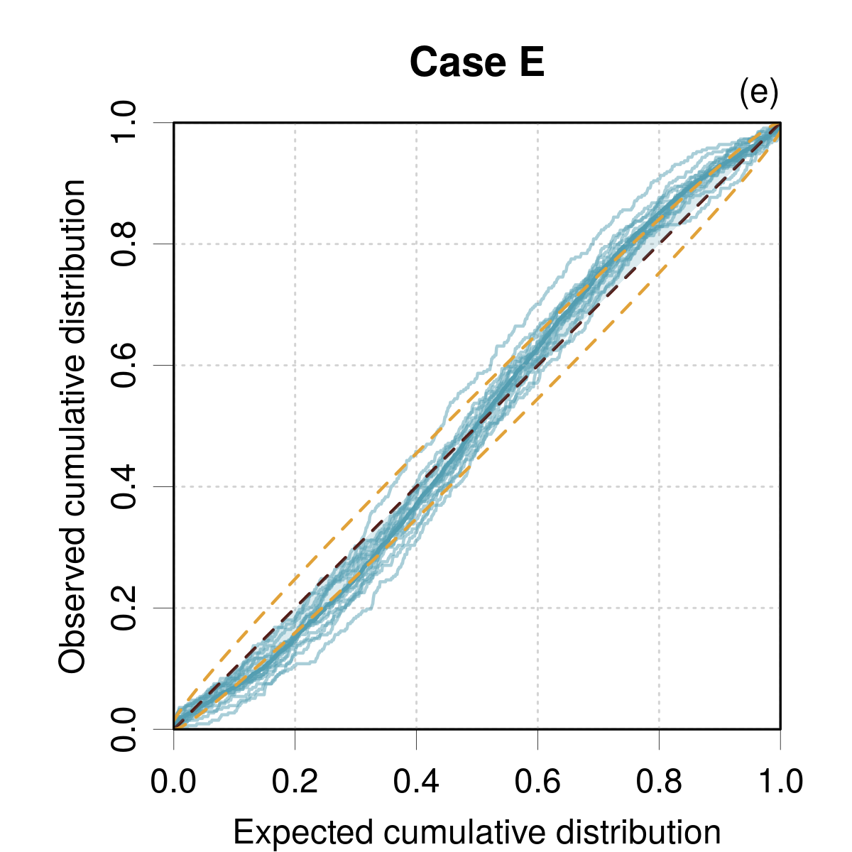
Figure 9: Conditional calibration curves in $X$ space for cases A-F. The average calibration curve is a thick blue line, the conditional curves are thin blue lines. The reference line and its 95 % confidence interval are dashed red lines. The dataset has been split according to the binning of $X$ into 15 equal-counts sets.

III.4.3 Local Z-Variance analysis in input feature space

As the LZV/LZISD analysis in $u_{E}$ space was used to validate consistency, one can perform a LZV of LZISD analysis in $X$ space to validate adaptivity. Here again, the LZISD analysis offers a more direct quantification of deviations. Both methods can be used for homoscedastic uncertainties.

The diagnostics provided by the LZISD analysis on the synthetic datasets are non-ambiguous (Fig. 10): Cases B, C and D stand out as having strong deviations from the reference line, while Cases A, E and F present a good adaptivity, as observed on the “$Z$ vs $X$” plots.

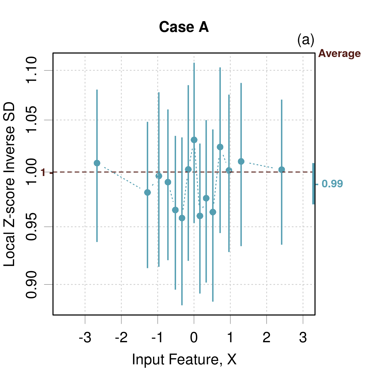
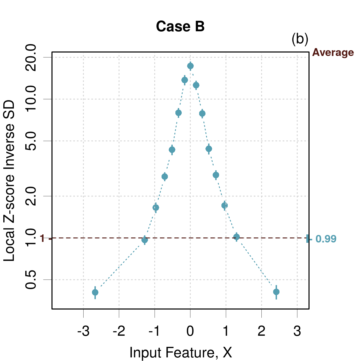
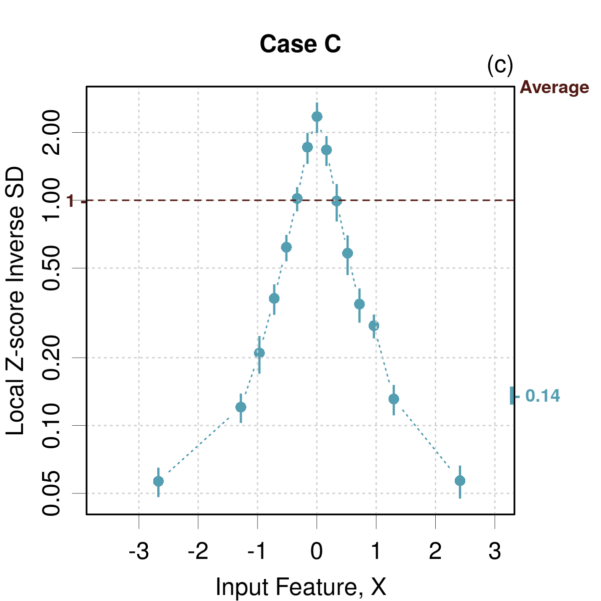
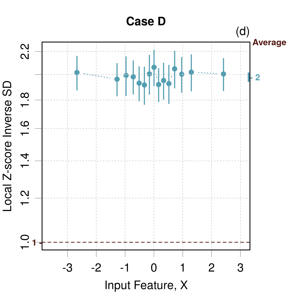
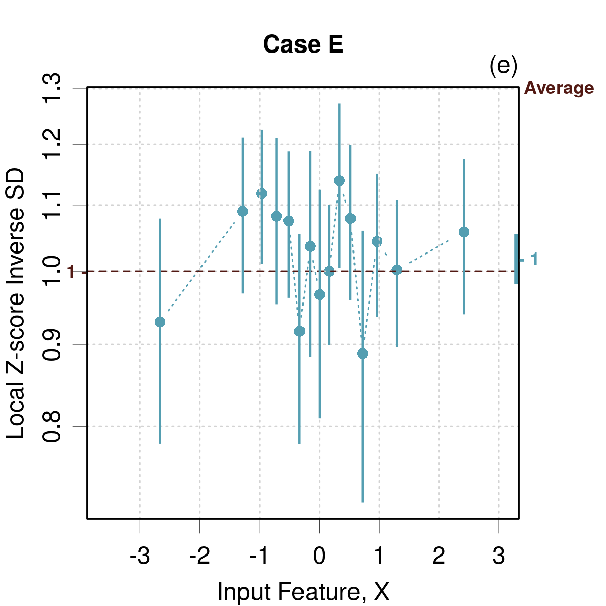
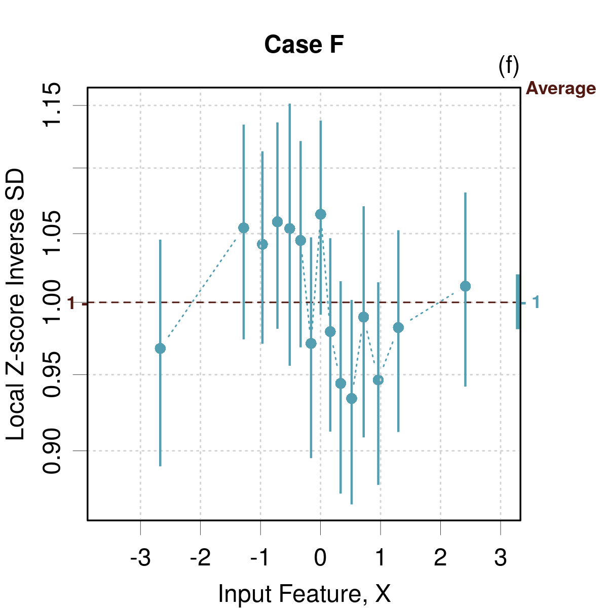
Figure 10: LZISD analysis against $X$ for cases A-F. The points are reported at the center of the bins. The error bars correspond to 95 % confidence intervals on the statistic. The value and error bar reported on the right axis corresponds to the statistic for the full dataset (Average).

III.4.4 Local Coverage Probability analysis in input feature space

Using the same binning for $X$ as used in the other methods, the LCP analysis (Fig. 11) provides results conform with those of the conditional calibration curves (Fig. 9). Here also, the hypothesis of a normal generative distribution used to build the probability intervals penalizes Case E, which can be solved by an appropriate choice of distribution (not shown).

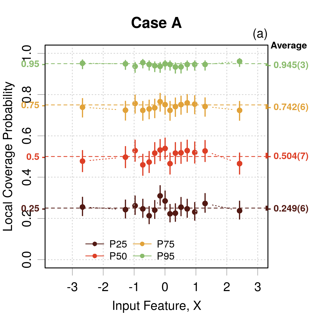
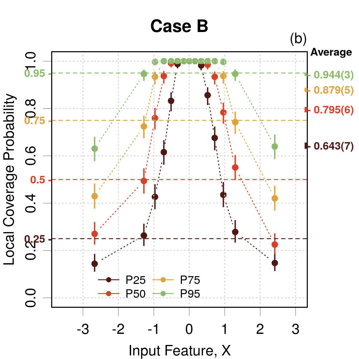
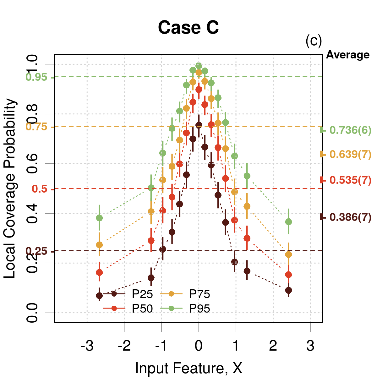
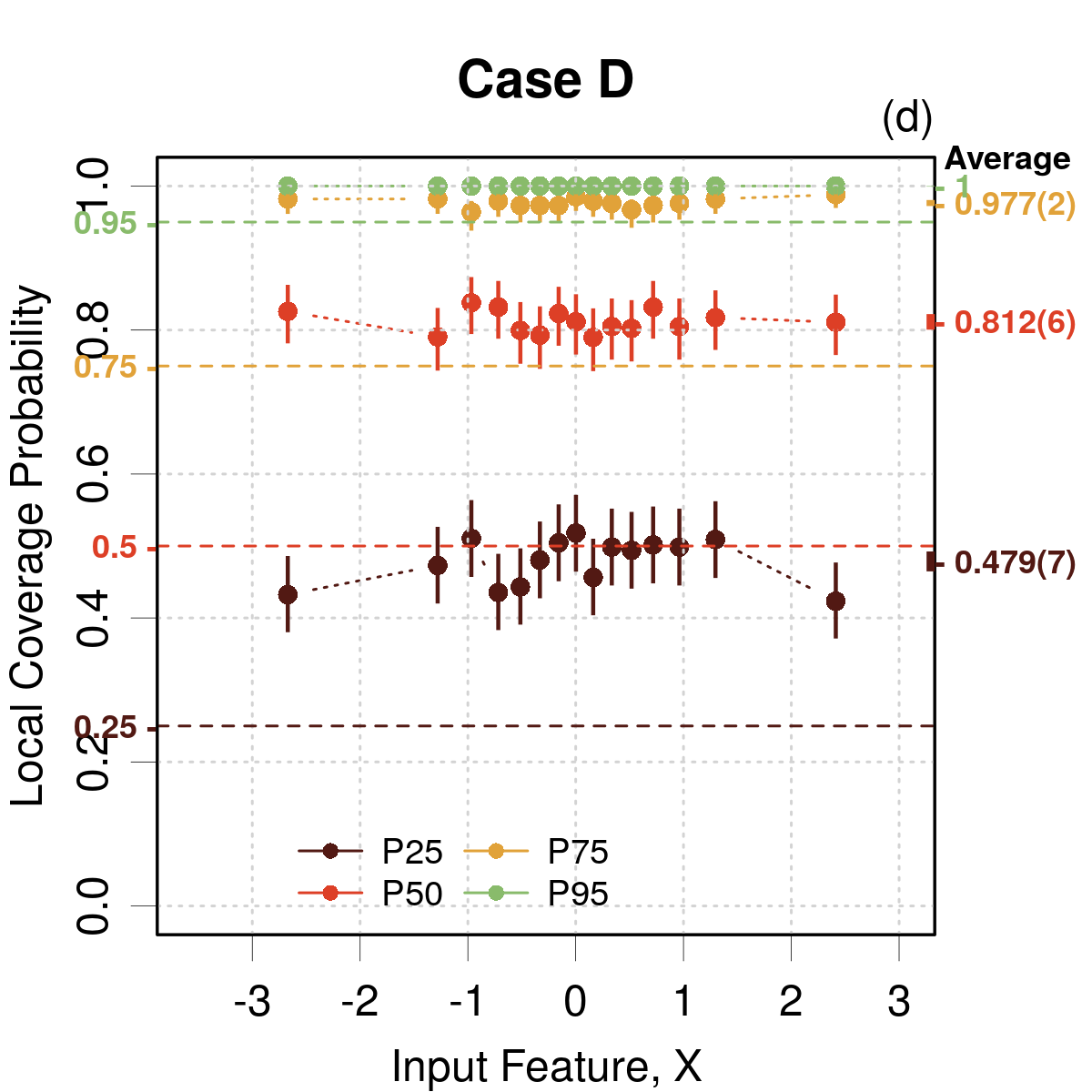
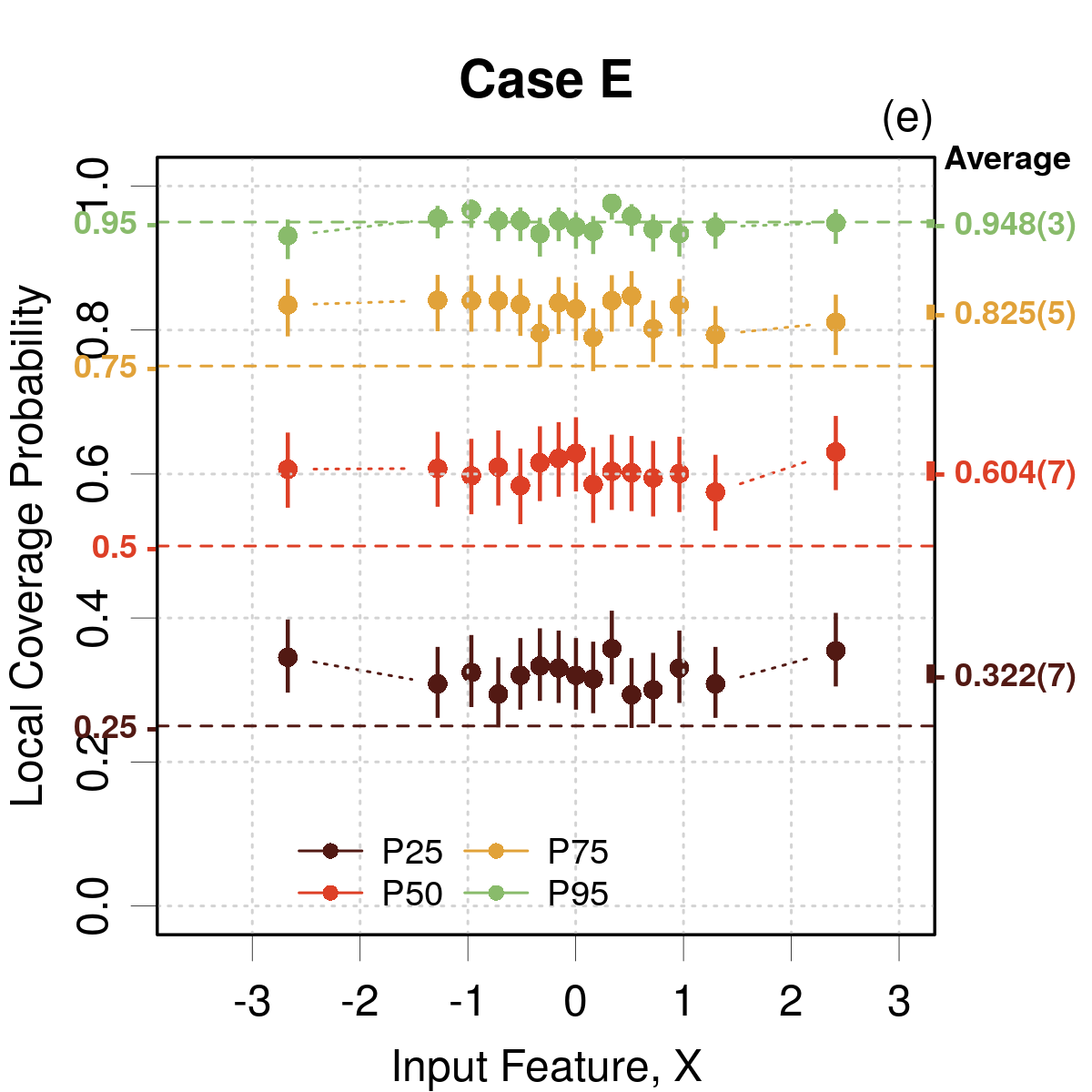
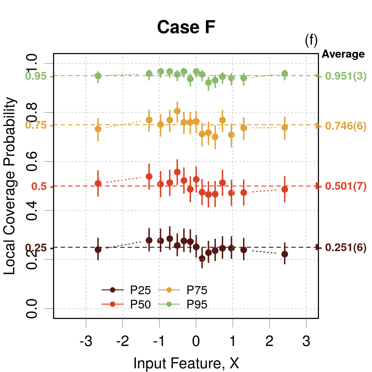
Figure 11: LCP analysis conditional to $X$ for cases A-F. The points are reported at the center of the bins. The error bars correspond to 95 % confidence intervals on the statistic. The value and error bar reported on the right axis corresponds to the statistic for the full dataset (Average).

III.4.5 Using latent distances or $V$ as conditioning variables

Although using one or several input features $X$ as conditioning variable is the most direct way to test adaptivity, it might not always be practical, for instance when input features are strings, graphs or images. In such cases, one might use instead a latent variable or the predicted property value $V$.

$X$ and $V$ are interchangeable only if the latter is a monotonous transformation of the former, but they might provide different adaptivity diagnostics if this is not the case. Using $V$ answers to the question: Are uncertainties reliable over the full range of predictions ?

The adaptivity analysis of the synthetic datasets using $V$ as a conditioning variable is presented in Appendix A. It shows that the non-monotonous shape of the $V=f(X)$ model might induce artifacts in the adaptivity analysis that can be difficult to interpret if the functional form of the model is unknown or complex.

III.5 Validation metrics

The present study focuses on graphical validation tools, but validation metrics(Maupin2018, ; Vishwakarma2021, ) are widely used in the ML-UQ literature. For instance, metrics have been designed for calibration curves(Kuleshov2018, ; Tran2020, ), reliability diagrams(Levi2020, ), and confidence curves(Scalia2020, ). These metrics are generally used to rank UQ methods, but they do not provide a validation setup accounting for the statistical fluctuations due to finite-sized datasets or bins. This is essential for small validation datasets and is not without interest for the conditional analysis of large ML datasets.

Pernot(Pernot2022a, ) introduced confidence bands for calibration curves that enables to identify significant deviations from the identity line, and also error bars for reliability diagrams, LZV and LCP analyses. This provides a basis to define upper limits for calibration metrics that can be used for validation purpose. In the present state of affairs, calibration metrics such as the expected normalized calibration error (ENCE)(Levi2020, ; Scalia2020, ; Vazquez-Salazar2022, ) or the area under the confidence-oracle (AUCO)(Scalia2020, ) cannot be used to validate consistency nor adaptivity and deserve further consideration beyond the purpose of this article.

IV Applications

The validation methods introduced in the previous sections are now applied to “real life” data coming from the materials science and physico-chemical ML-UQ literature. The choice of datasets enables to explore various aspects of a posteriori validation. It is not my intent in these reanalyses to criticize the analyzes nor the UQ methods presented in the original studies, but simply to show how the augmented set of validation methods proposed above might facilitate and complete the calibration diagnostics.

IV.1 Case PAL2022

The data have been gathered from the supplementary information of a recent article by Palmer et al.(Palmer2022, ). I retained 8 sets of errors and uncertainties before and after calibration by a bootstrap method, resulting from the combination of two materials datasets (Diffusion, $M=2040$ and Perovskites, $M=3836$) and several ML methods (RF, LR, GPR….). The datasets are tagged by the combination of both elements: for instance, Diffusion_RF is the dataset resulting from the use of the Random Forest method on the Diffusion dataset. The reader is referred to the original article for more details on the methods and datasets.

As only the errors $E$ and uncertainties $u_{E}$ are available, it is not possible to test adaptivity for this dataset. My aim here is mainly to compare the performance of reliability diagrams and LZISD analysis against the binning strategy, and to compare their results to confidence curves with the probabilistic reference.

IV.1.1 Average calibration

As a first step, I estimated for each dataset the mean of z-scores and their variance to appreciate the average impact of the calibration method. Fig. 12 summarizes the results. It can be seen that calibration leaves the mean z-score unchanged or improves it (the calibrated value is closer to zero). After calibration, the mean z-scores are not always null, but small enough to consider the error sets to be unbiased. The calibration effect is more remarkable for $\mathrm{Var}(Z)$: all the 95 % confidence intervals for $\mathrm{Var}(Z)$ after calibration overlap the target value ($1.0$), except for Perovskite_LR with a very small residual gap.

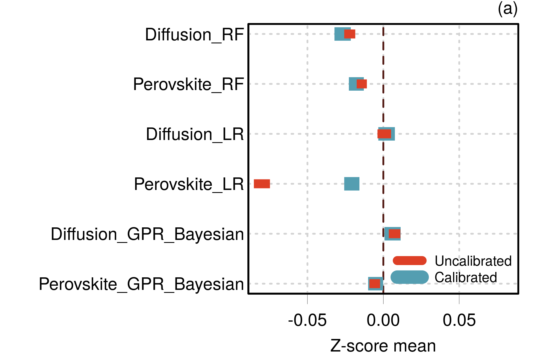
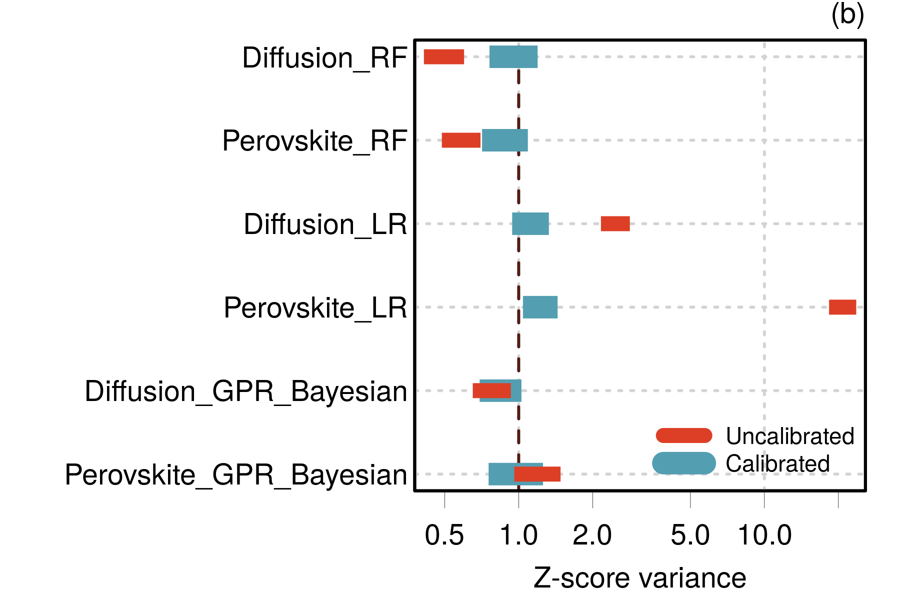
Figure 12: Case PAL2022: mean and variance of z-scores for all datasets before and after calibration. The horizontal bars represent 95 % confidence intervals.

IV.1.2 Consistency

Consistency can be checked by reliability diagrams, LZISD analysis and confidence curves with probabilistic reference. In absence of information on the generative distribution(s), it is best to avoid conditional calibration curves in this example. Before analyzing the datasets, it is important to point out the impact of the binning strategy on the conclusions drawn from reliability diagrams and LZISD analysis. In their study, Palmer et al. define 15 intervals forming a regular grid in $u_{E}$ space, with some adaptations described in Appendix B. This is different from the usual strategy consisting in designing bins with identical counts.(Scalia2020, ; Pernot2022a, ) Besides, considering the size of the datasets, 15 bins might not be enough to reveal local consistency anomalies. The impact of the binning strategy is explored in Appendix B, where an adaptive binning strategy is designed to combine both approaches. When using the log-scale for uncertainty binning, this adaptive strategy is efficient to reveal local consistency anomalies that do not always appear in the original reliability diagrams.

Calibrated Random Forest.

The LZISD analysis and reliability diagrams are shown in Fig. 13 for both datasets. The effect of calibration is well visible on those graphs when comparing the red dots (uncalibrated) to the blue ones (calibrated). For both datasets, consistency after calibration is rather good, except for the small uncertainty values (below 0.25 eV for Diffusion and 0.15 eV for Perovskite). The legibility is better on the LZISD analysis, which provides directly an overestimation value of 50 % of the uncertainties around 0.2 eV for Diffusion and up to 100 % around 0.08 eV for Perovskite.

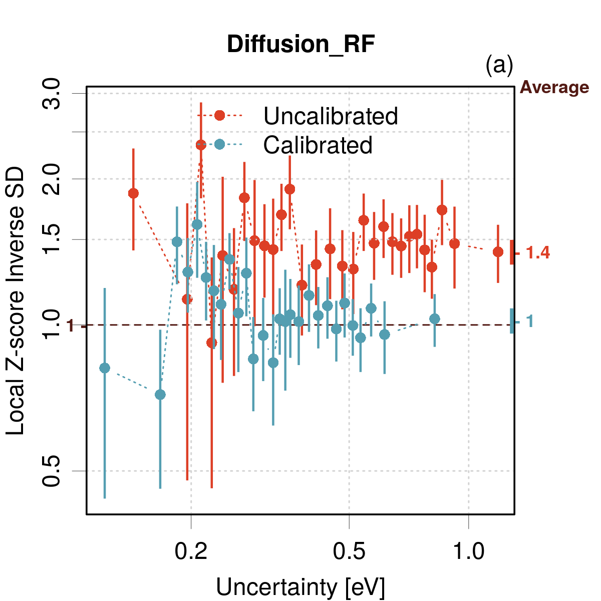
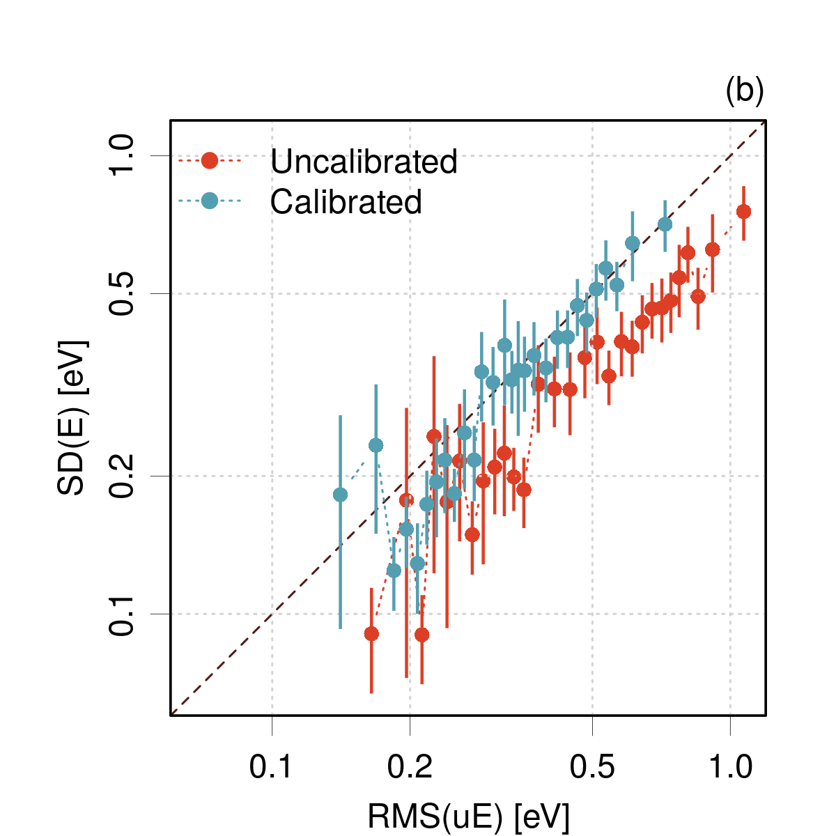
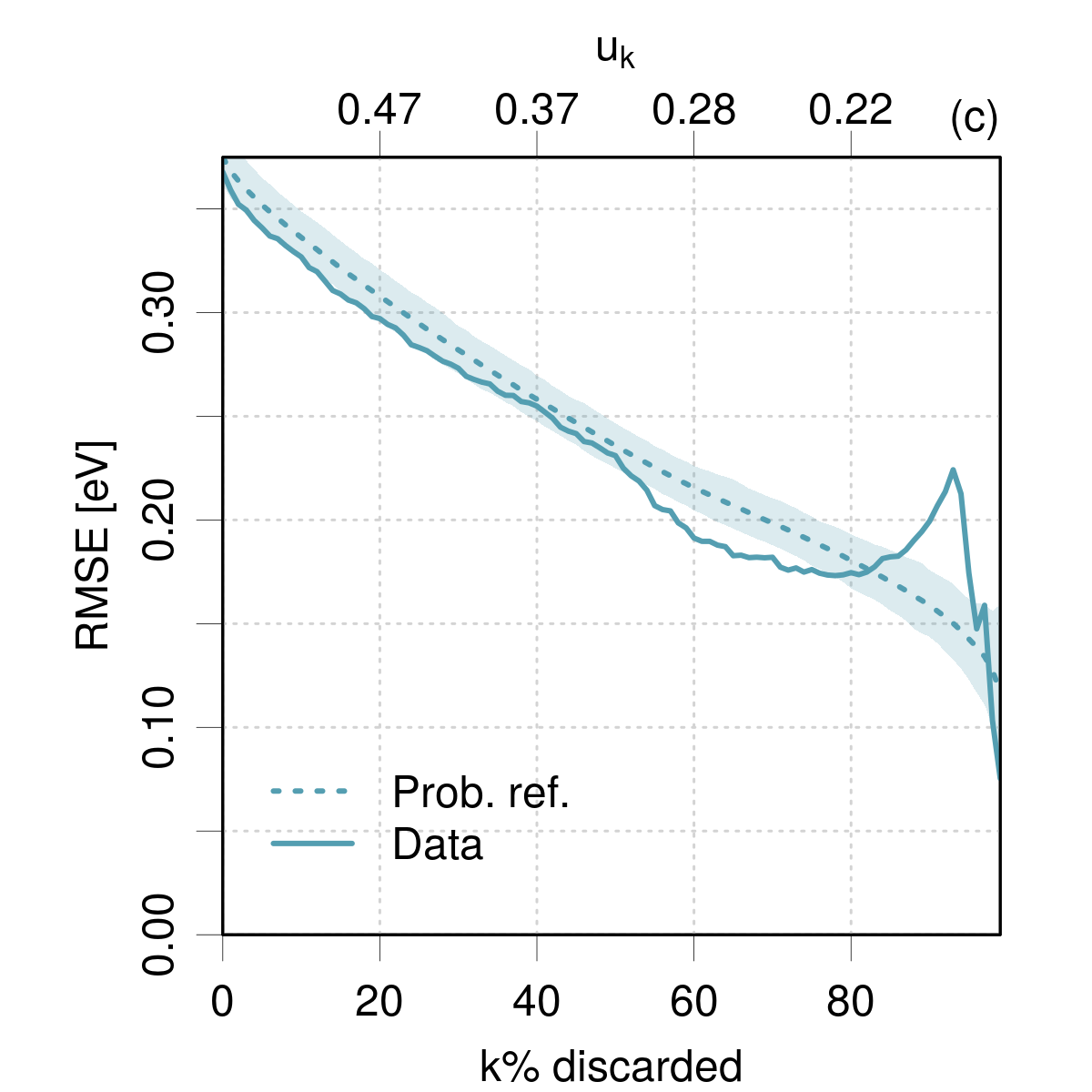
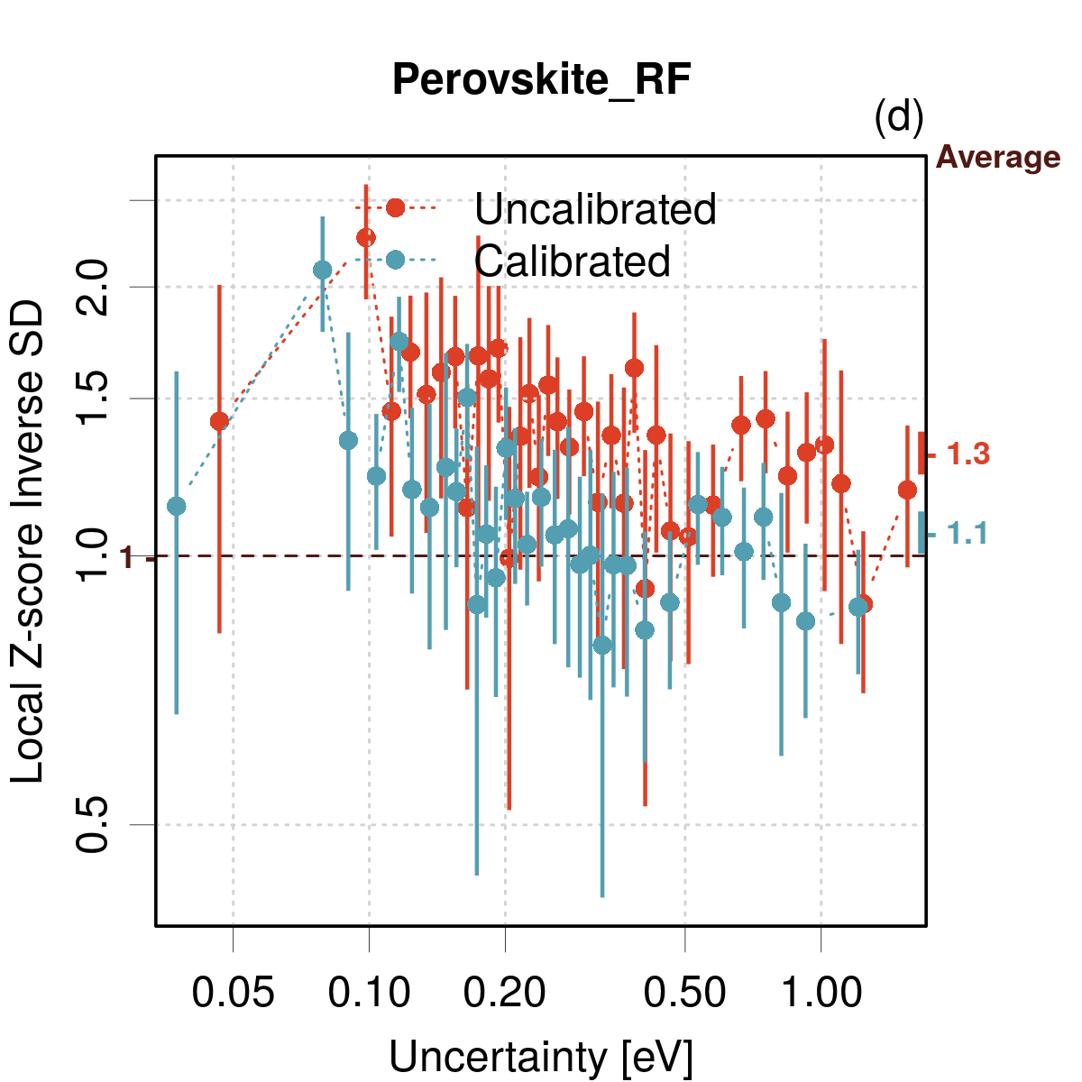
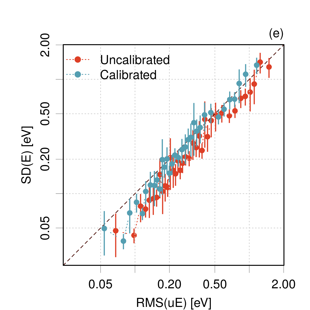
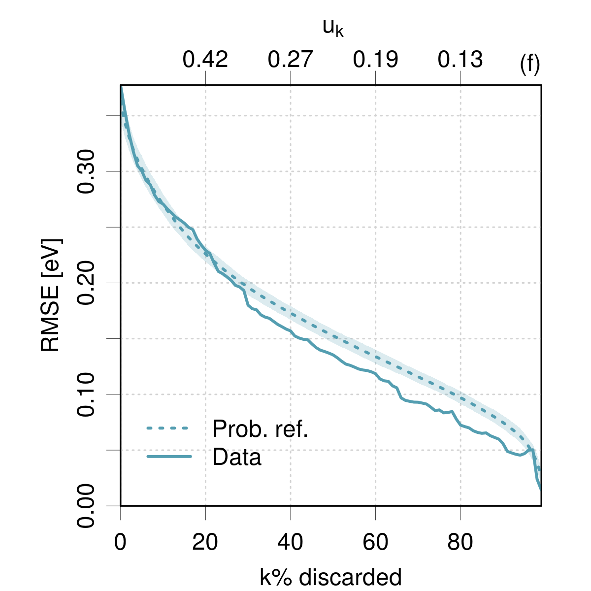
Figure 13: Case PAL2022: UQ validation for random forests examples.

The confidence curves in Fig. 13 confirm this diagnostic, as they lie close to the reference for large uncertainties and start to deviate from it at smaller uncertainties. The non-linear scale of threshold values $u_{k}$ at the top of the plot helps to locate the anomalies in uncertainty space.

Calibrated Linear Ridge regression.

Calibration and consistency of linear ridge regression results are assessed in Fig. 14. The effect of calibration is noticeable over the whole uncertainty range, except at large uncertainties for the Diffusion dataset, where the situation is worsened by calibration. In this area, the uncertainties are overestimated by a factor about 2. At smaller uncertainties, the consistency is far from perfect, with areas of underestimated uncertainties around 0.3 eV and 0.5 eV, compensating for the overestimated values at large uncertainty. The confidence curve displays the problem at large uncertainty values, but is less legible at smaller uncertainties.

For the Perovskite dataset, consistency is not reached either, with a compensation between overestimated and underestimated uncertainty areas. The confidence curve is notably deviating from the reference curve.

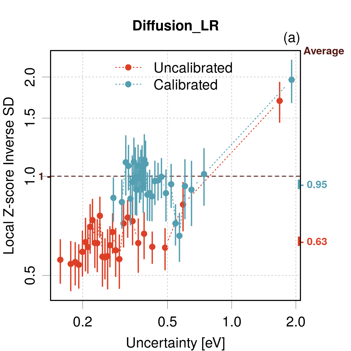
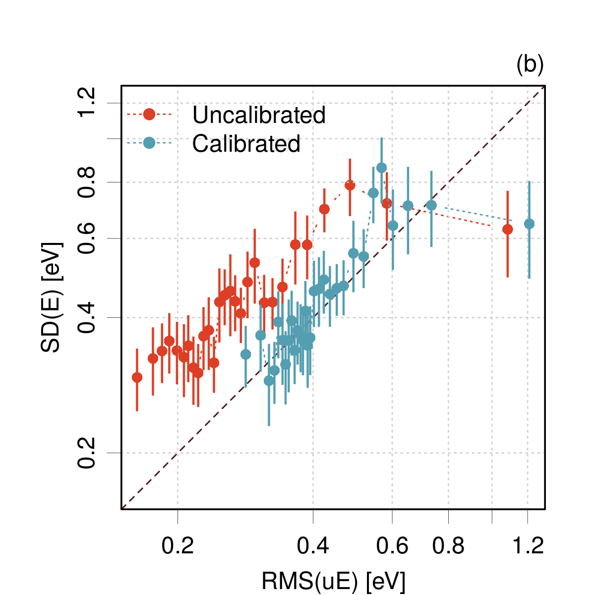
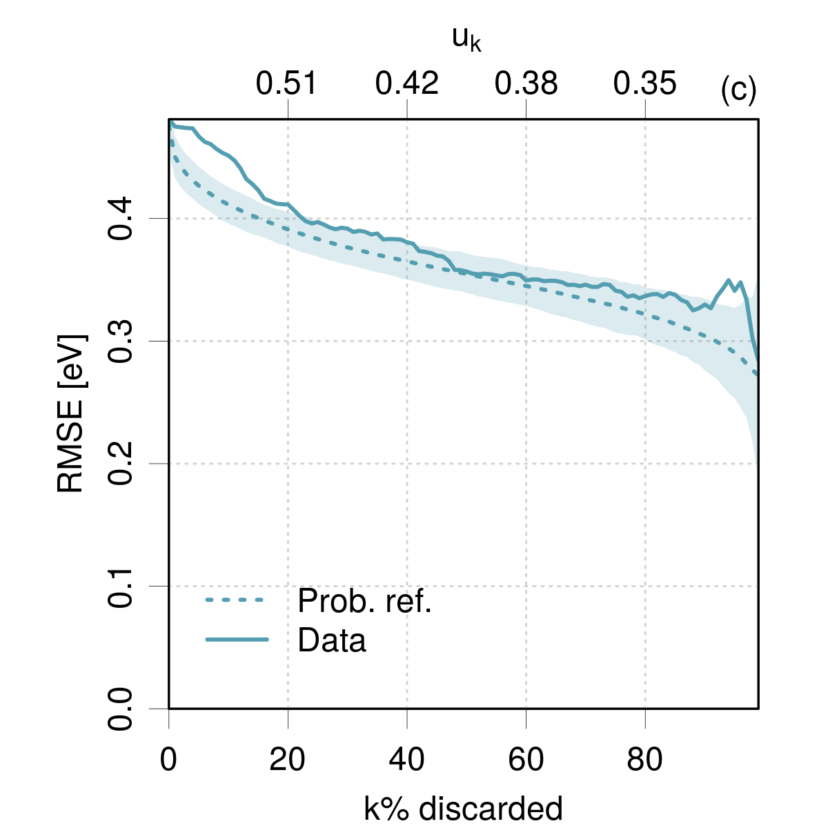
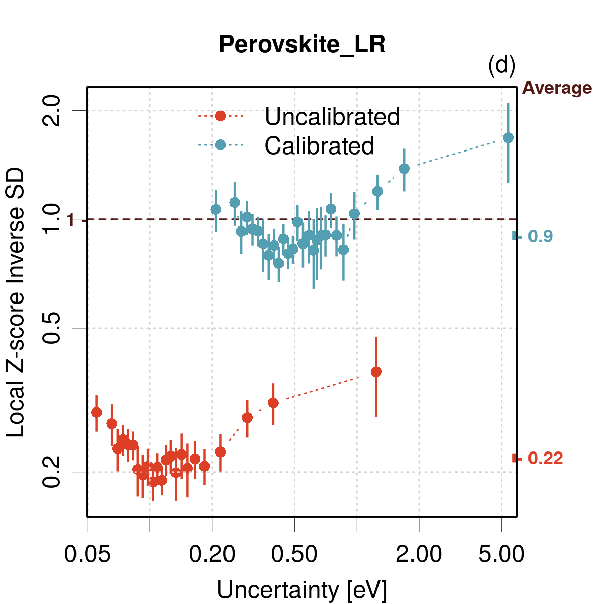
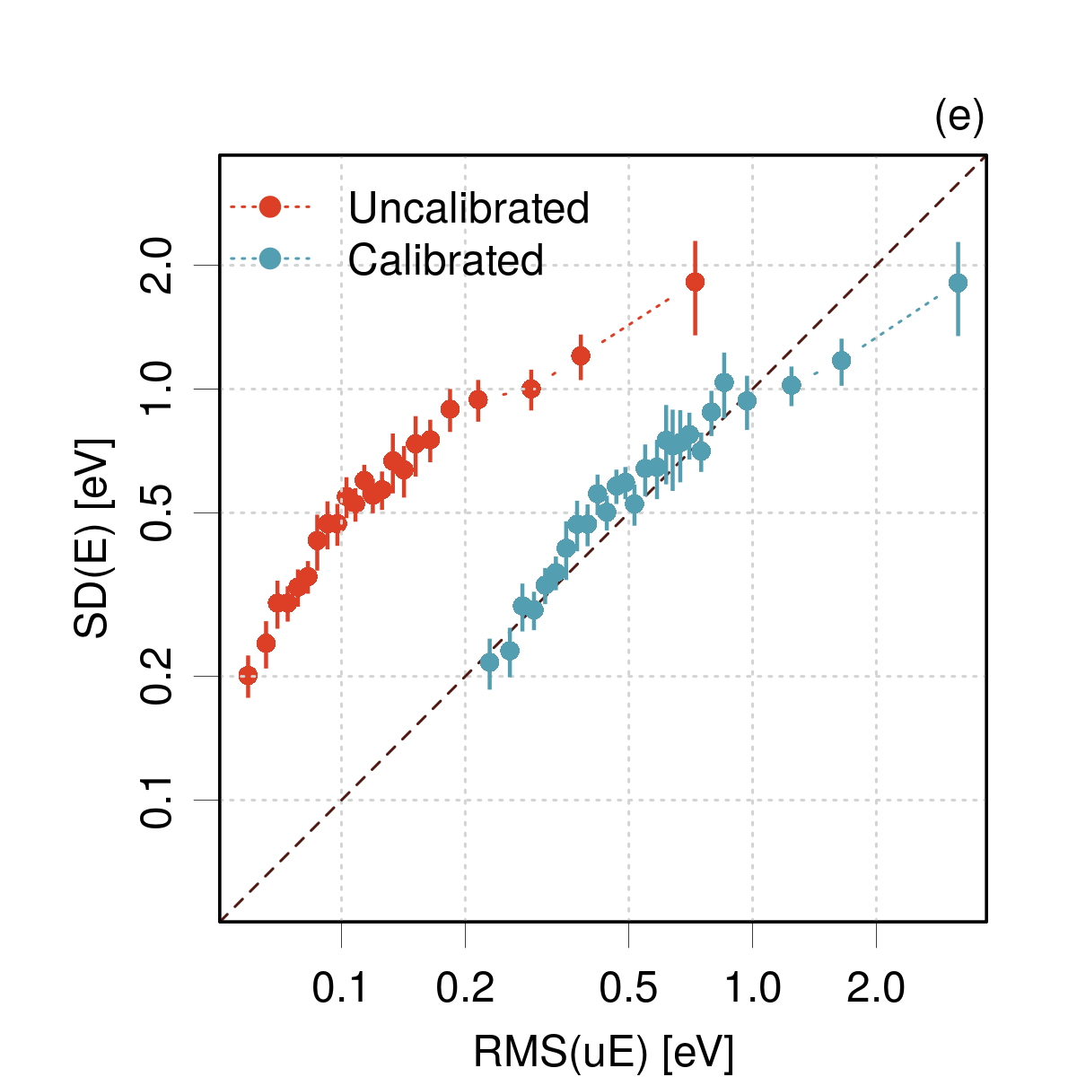
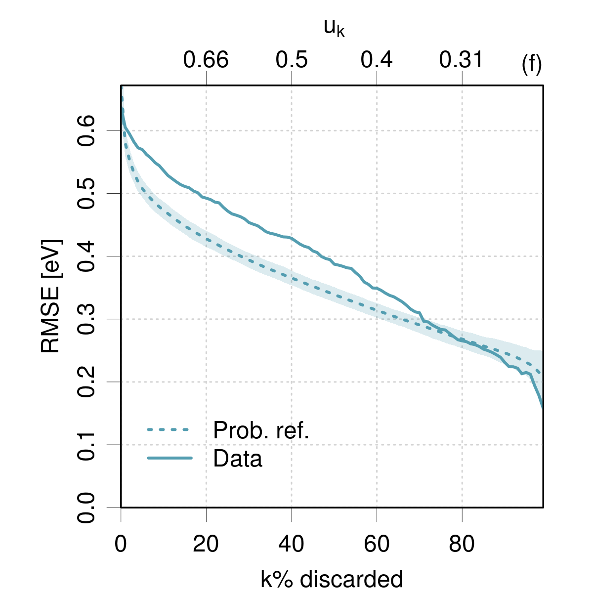
Figure 14: Case Pal2022: UQ validation for linear ridge regression examples.

Calibrated Gaussian Process Regression.

One considers here the calibration results of a Gaussian Process regression with its Bayesian UQ estimate. It is possible to go quickly to the conclusion that consistency is not achieved.

For the Diffusion dataset, all three graphs (Fig. 15) concur to reject consistency. The confidence curve even suggests that it would not be reasonable to base an active learning strategy on these uncertainties.

In the case of Perovskite one observes a nugget of data with tiny errors and largely overestimated uncertainties, that was identified by the adaptive binning strategy (Appendix B). A zoom over the remaining data (not shown) reveals an heterogeneous situations with small areas of underestimation (below 0.2 eV) and overestimation (around 0.3 eV and 0.6 eV). The confidence curve deviates considerably from the reference and falls unexpectedly to zero at small uncertainties, a consequence of the aforementioned data nugget.

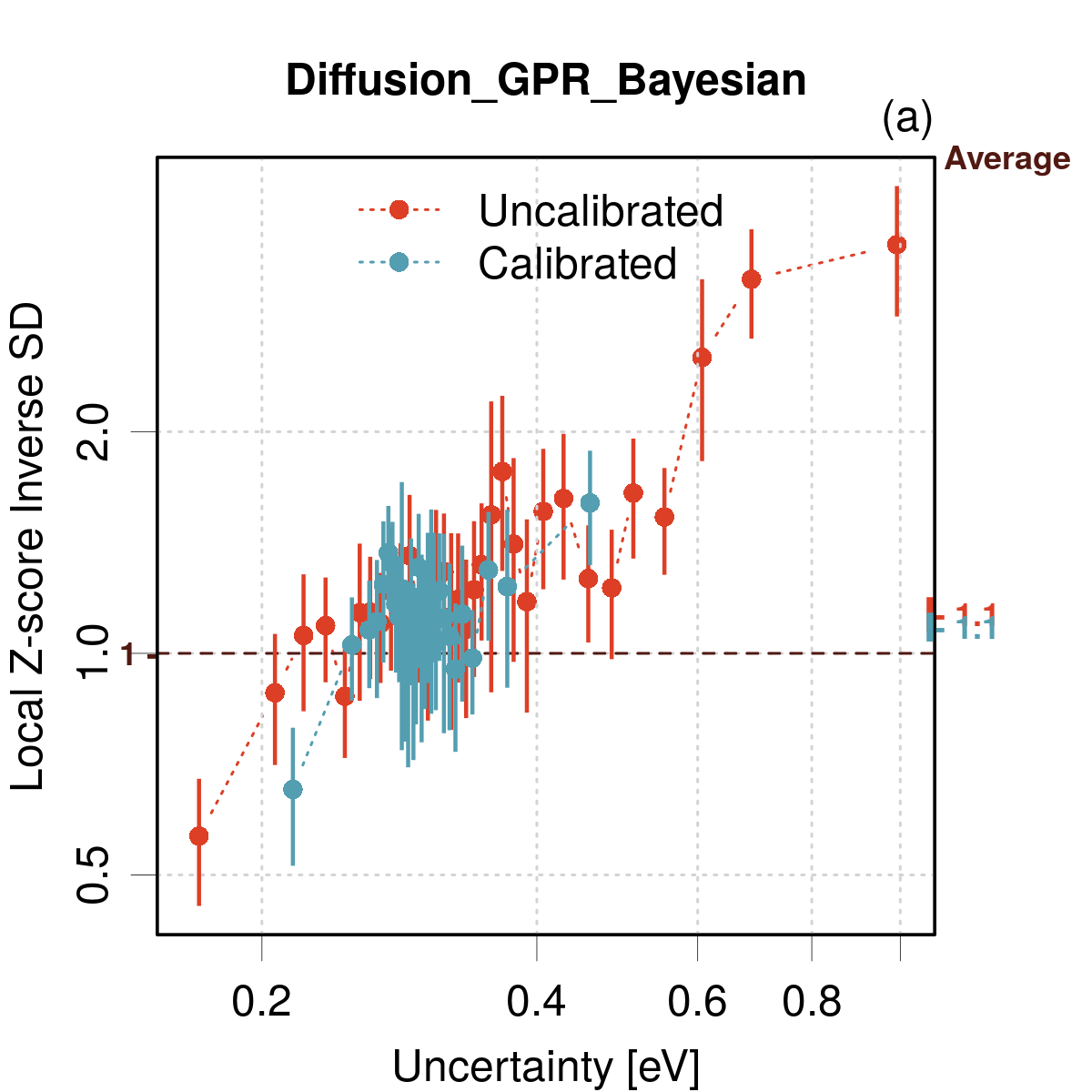
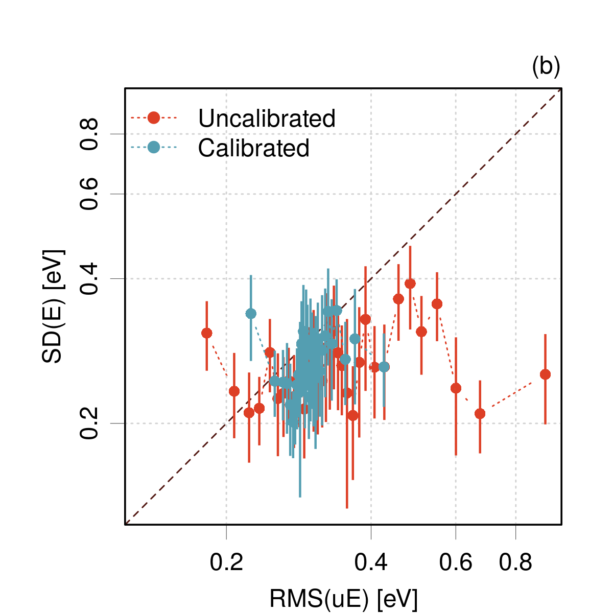
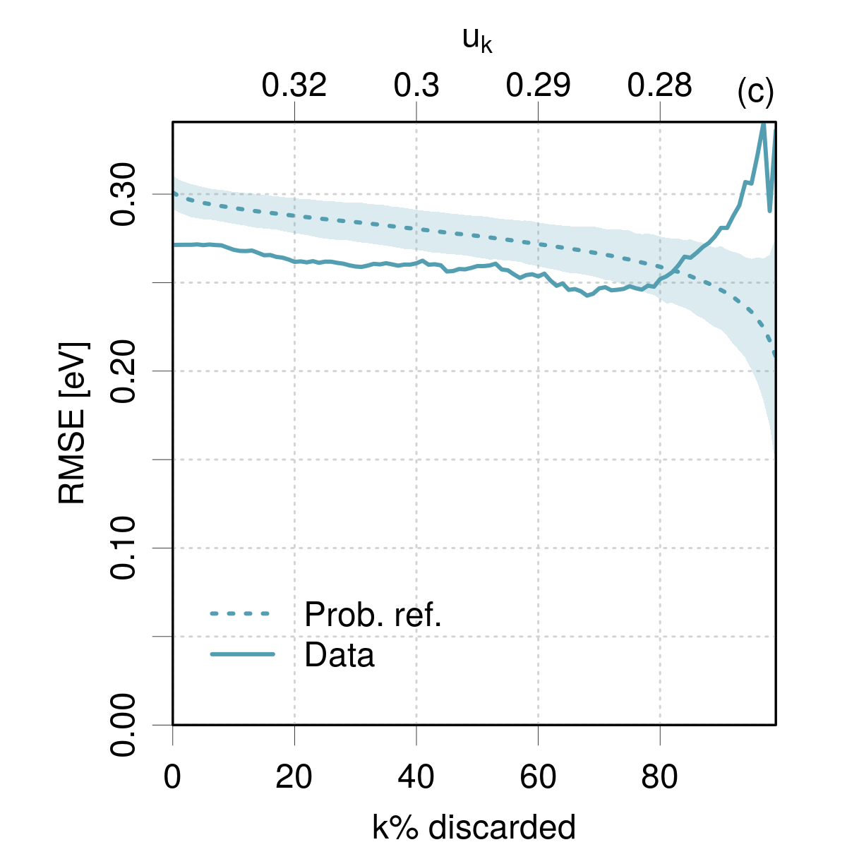
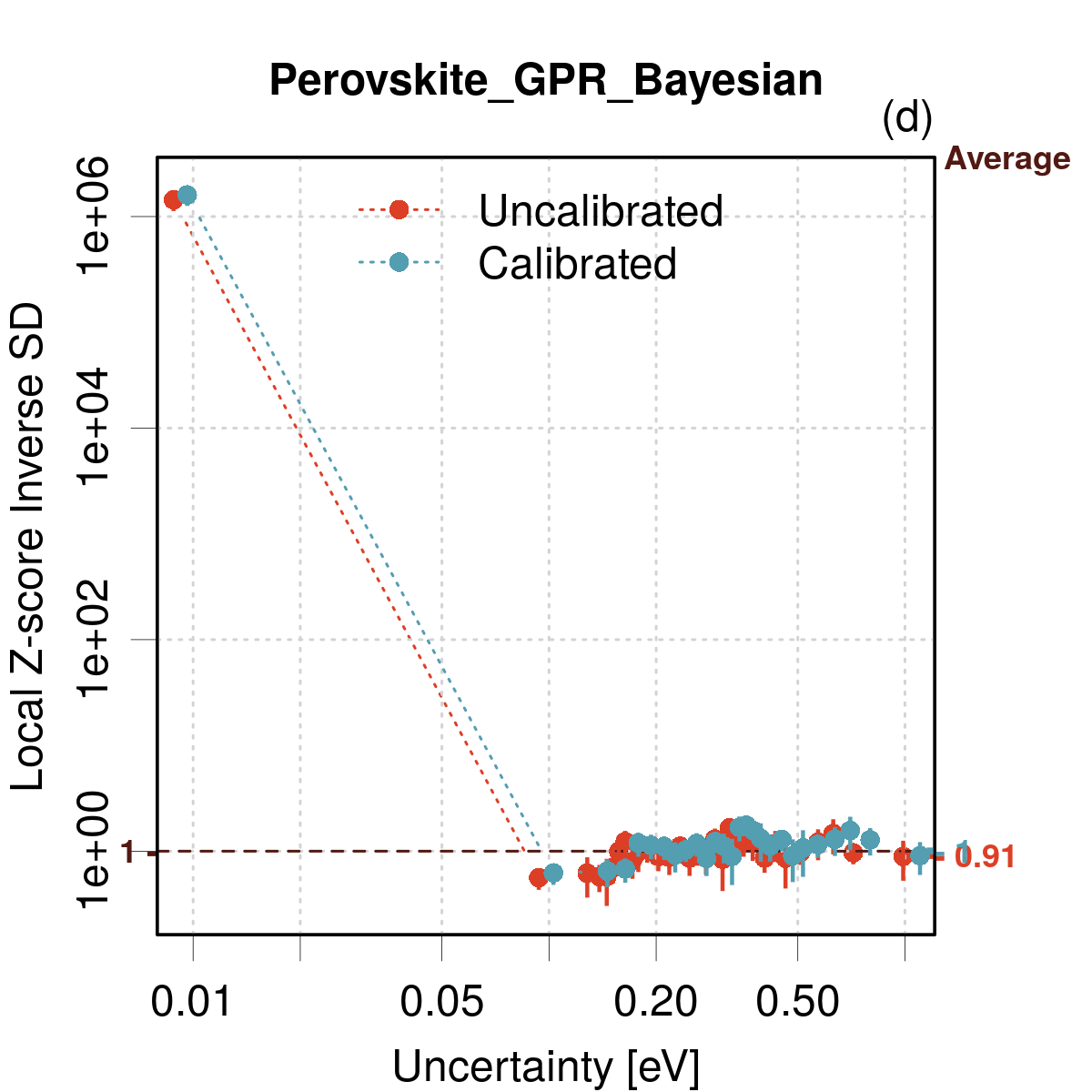
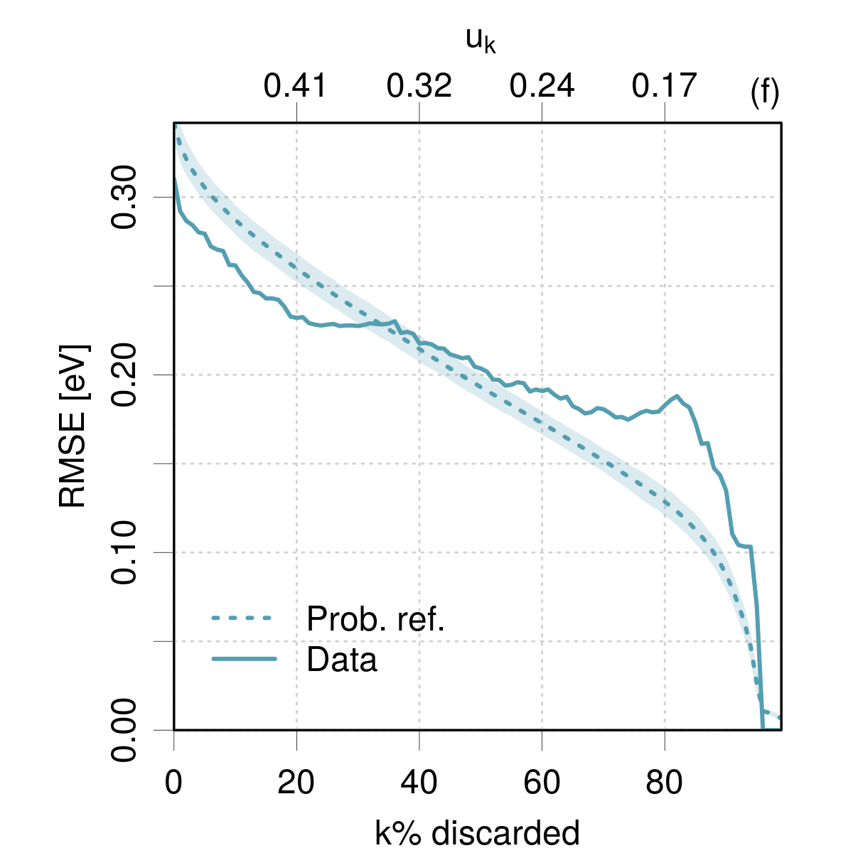
Figure 15: Case PAL2022: UQ validation for gaussian process regression examples.

Conclusion.

The reanalysis of these data shows that the reliability diagrams presented in the original article with a small number of bins and no error bars are often overoptimistic. Using an adaptive binning strategy in log-uncertainty, conditional calibration appears heterogeneous for all datasets, meaning that consistency is not achieved despite a rather good average calibration.

The uncertainties are at worst within a factor two of their ideal value, a level that has to be contrasted with their intended application. The confidence curves show that not all ML methods provide reliable uncertainties for active learning.

IV.2 Case BUS2022

The data presented in Busk et al.(Busk2022, ) have been kindly collated by Jonas Busk for the present study. In their article, Busk et al. extend a message passing neural network in order to predict properties of molecules and materials with a calibrated probabilistic predictive distribution. An a posteriori isotonic regression on data unseen during the training is used to ensure calibration. For UQ validation, these authors used the more or less standard trio of reliability diagrams, calibration curves (named quantile-calibration plot) and MAE-based confidence curves with the oracle reference. Note that they duly express a reserve about using the oracle: “However, we do not expect a perfect ranking…”(Busk2022, ).

Considering the validation results published for the QM9 dataset in Fig. 2 of the original article, a few questions arise: (1) what is causing the imperfect calibration curve ?; (2) if this is a wrong distribution hypothesis, how does it affect the MAE-based confidence curve ?; (3) how is the confidence curve analysis modified if one uses the RMSE statistic and the probabilistic reference ?; and, (4) what is the diagnostic for adaptivity? The present reanalysis aims to answers these questions.

IV.2.1 Reanalysis of the QM9 dataset

The QM9 dataset consists of 13 885 predicted ($V,u_{V}$), reference ($R$) atomization energies, and molecular formulas. These data are transformed to $C=\left\{X,E,u_{E}\right\}$ according to Sect. II.1.1, where $X$ is the molecular mass generated from the formulas. One should thus be able to test calibration, consistency and adaptivity. Average calibration is readily assessed ($Var(Z)=0.96(2)$).

It is always instructive to inspect the raw data through “$E$ vs $u_{E}$” and “$Z$ vs $X$” plots to get a global appreciation of the link between these quantities (Fig. 16). One sees in Fig. 16(a) that the data points are neatly distributed between the $E=\pm 3u_{E}$ guiding lines, and the 0.025 and 0.975 running quantile lines seem to follow closely the $E=\pm 2u_{E}$ lines up to $uE\simeq 0.05$. Above this value, the uncertainties seem overestimated and the errors are somehow biased toward the positive values. However, this concerns a very small population (about 95 points) and filtering them out does not affect significantly the calibration statistics presented below. The problem might be simply due to the sparsity of the data in this uncertainty range.

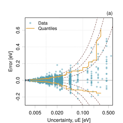
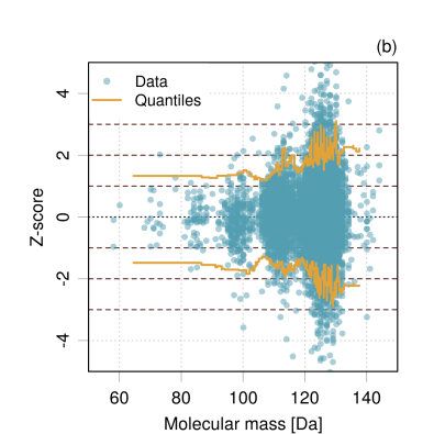
Figure 16: Case BUS2022: (a) errors vs. uncertainty; (b) z-scores vs. prediction.

The “$Z$ vs $X$” plot in Fig. 16(b) using molecular masses enables to check if calibration is homogeneous in mass space. The shape of the running quantile lines indicate that uncertainties are probably overestimated for masses smaller than the main cluster around 125-130 Da, evolving to a slight underestimation above this peak. Depending on its amplitude, this systematic effect might be problematic, and it hints at a lack of adaptivity. A quantitative analysis of this feature is presented below.

In a first step, calibration analyses are done to reproduce the Fig. 2 of the original article: reliability diagram with 10 equal-counts bins [Fig. 17(a)], calibration curve with the normal hypothesis [Fig. 17(b)] and MAE-based confidence curve (replacing the unsuitable oracle by the probabilistic reference) [Fig. 17(c)]. Then, further analyses are performed to complement the information provided by the first set: LZISD analysis in uncertainty and $V$ space [Fig. 17(d,e)], and RMSE-based confidence curve [Fig. 17(f)].

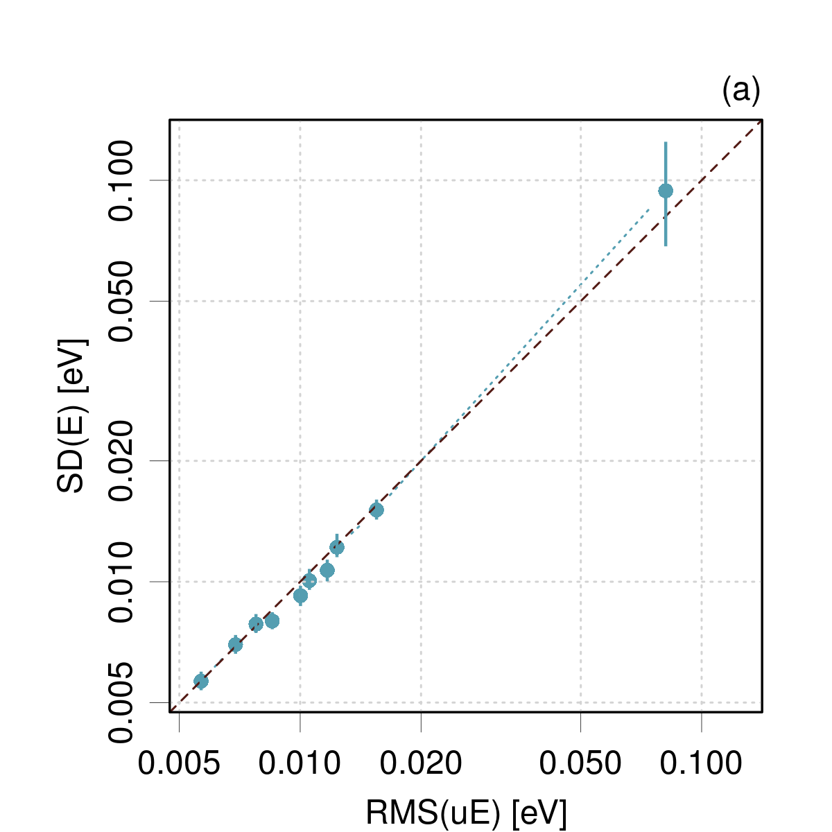
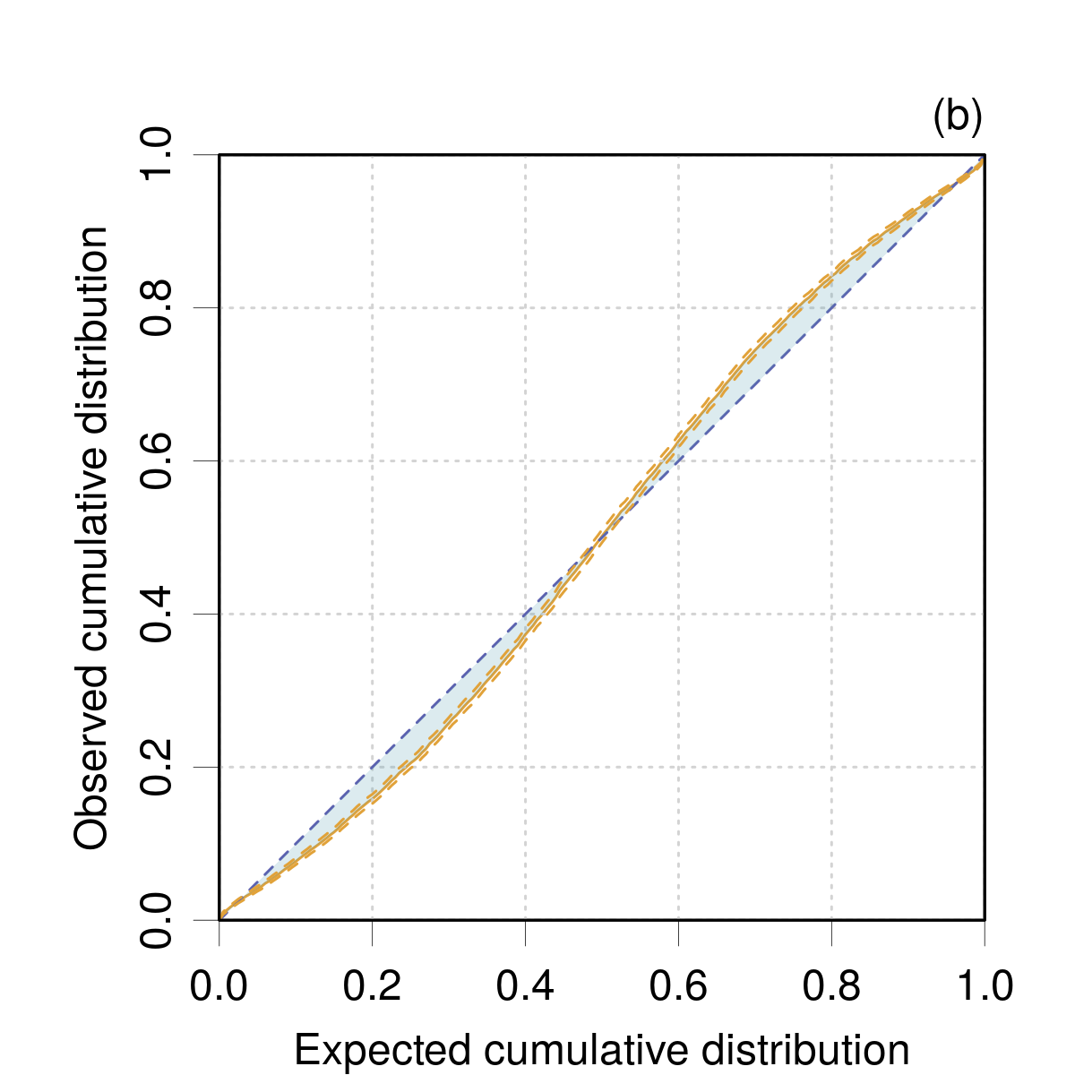
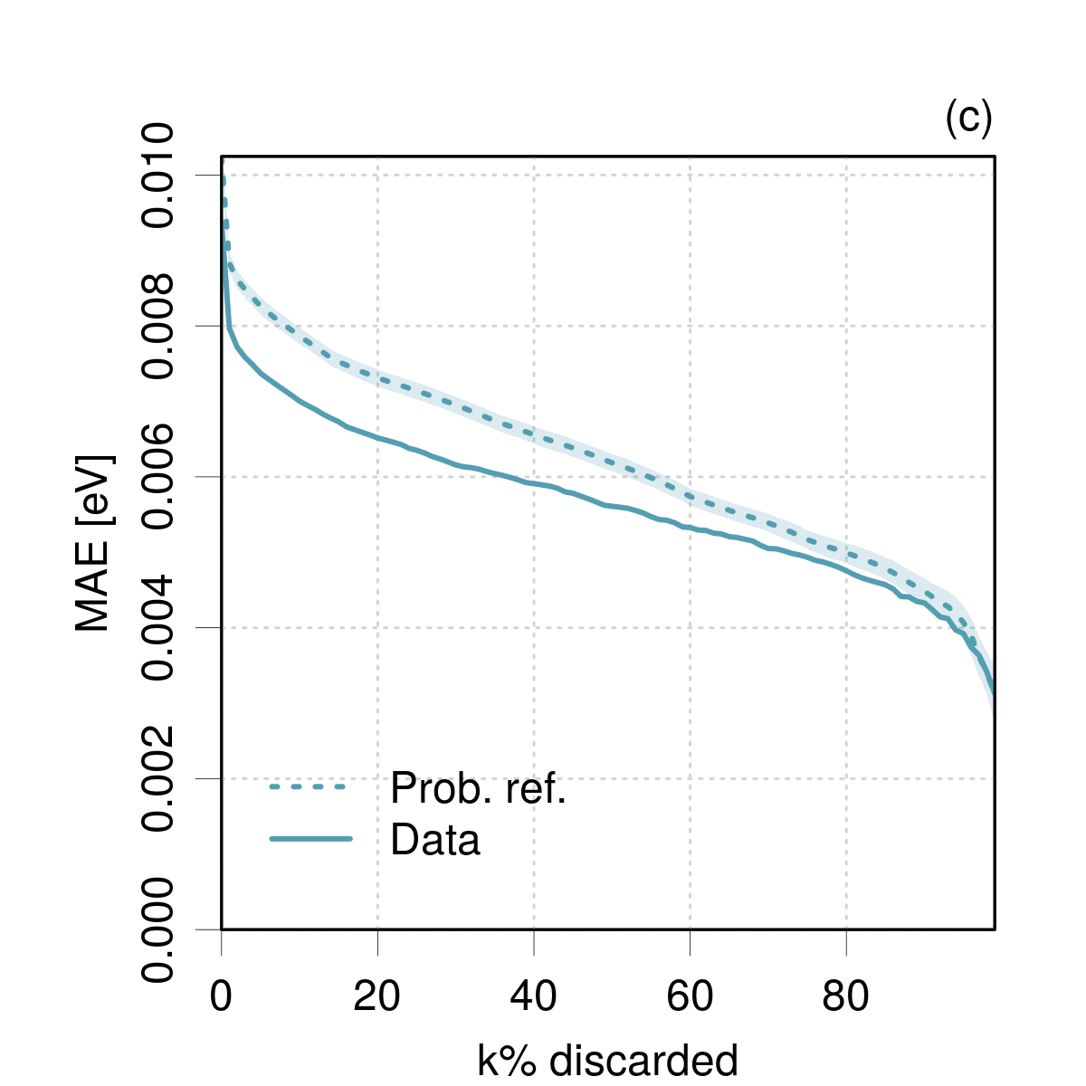
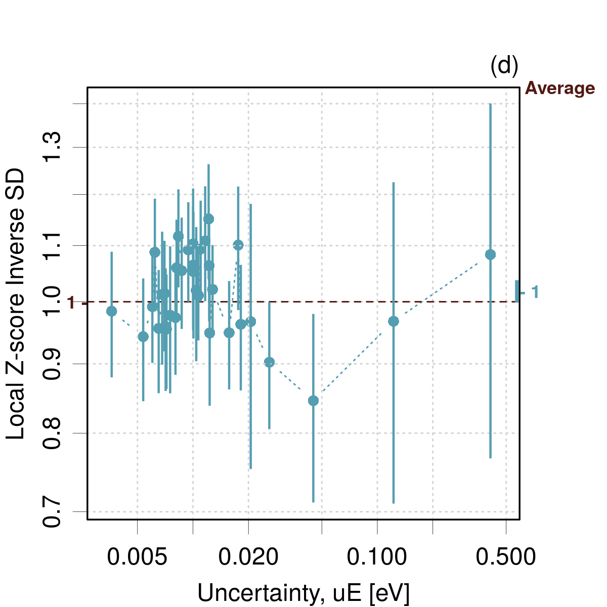
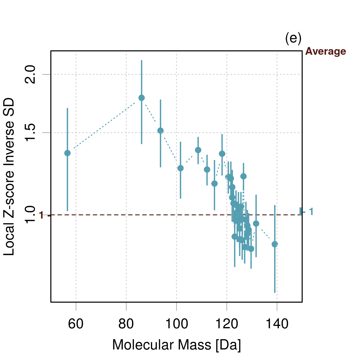
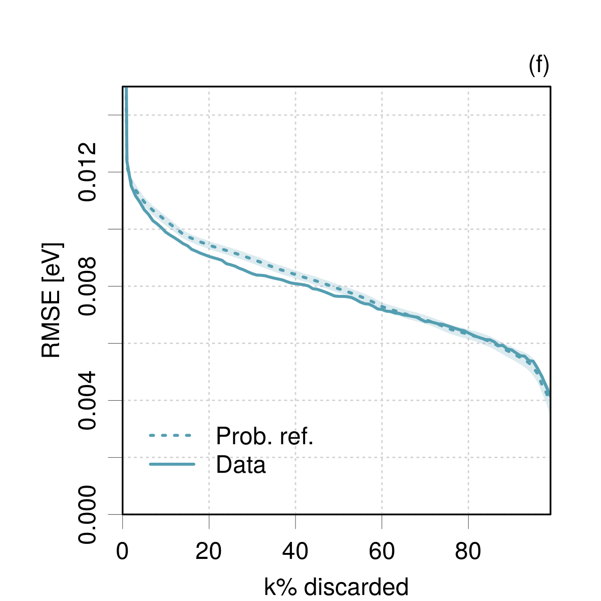
Figure 17: Case BUS2022: validation plots. (a) reliability diagram with 10 equal-counts bins; (b) calibration curve; (c) MAE-based confidence curve; (d) LZISD analysis vs. $u_{E}$, with adaptive binning strategy; (e) LZISD analysis vs. $V$, with adaptive binning strategy; (f) RMSE-based confidence curve (the data curve has been truncated at 0.015 eV, but it decreases sharply from 0.031 eV).

The reliability diagram [Fig. 17(a)] does not enable to see any major problem and would lead us to conclude that the data are consistent. However, the calibration curve [Fig. 17(b)] is not perfect. Considering the good consistency provided by the reliability diagram, one should conclude that there is probably a distribution problem, i.e., the generative distribution of errors that is used to build the probabilistic reference curve should not be normal. Moreover, the confidence curve [Fig. 17(c)] is not very close to the probabilistic reference, which, assuming a good consistency, points also to a problem of distribution, as the MAE-based probabilistic reference is sensitive to the choice of distribution. This distribution problem is analyzed more specifically below (Sect. IV.2.2).

A LZISD analysis with an adaptive binning strategy is performed to compare with the original reliability diagram [Fig. 17(d)]. Indeed, one observes some discrepancies: overestimation and underestimation of $u_{E}$ go locally up to 15 %. There is notably an overestimation trend around 0.01 eV. This feature is also present in the reliability diagram, but it is more difficult to visualize small deviations on a parity plot.

The LZISD analysis against the molecular mass [Fig. 17(e)] confirms and quantifies what has been observed in [Fig. 16(b)]: an overestimation between 40 and 80 % at masses below 120 Da, and a slight underestimation by about 20 % above 130 Da (although there are too few data in this range to conclude decisively). Uncertainties are therefore mostly reliable for the main mass peak between 120 and 130 Da, but not outside of this range. This heterogeneity of calibration and lack of adaptivity is not observable in the other validation plots.

Finally, a RMSE-based confidence curve is reported in Fig. 17(f). It has been truncated at 0.015 eV, but drops sharply from 0.031 eV because of the small set of large positive errors corresponding to the largest uncertainties [Fig. 16(a)]. This confidence curve shows a much better agreement with the probabilistic reference than the MAE-based one, albeit there is still a mismatch due to the consistency defects observed in the LZISD analysis and/or to the distribution problem mentioned above.

IV.2.2 Non-normality of the generative probabilistic model

The deviations of the calibration curve observed in Fig. 17(b) correspond neatly to observations made for one of the synthetic datasets (Case E) when drawing error from a Student’s-t distribution with four degrees of freedom and comparing the percentiles with a normal reference [Fig. 1(e)]. Indeed, if one substitutes the normal reference in the calibration plot by a $t_{\nu=4}$ reference, one obtains a perfect calibration curve [Fig. 18(a)].

One can consider two major sources of non-normality in this example: the Bayesian model using an inverse-gamma prior on the uncertainty variable(Soleimany2021, ; Busk2022, ), and/or the small size of the ensemble of neural networks ($n=5$).(Busk2022, ) The latter would explain perfectly the observed four degrees of freedom (see Sect. II.1.3). Note that averaging over small ensembles is expected to affect also $\mathrm{Var}(Z)$, but, in the present case, this is corrected by the a posteriori calibration stage, leaving only a distribution effect.

Assuming a $t_{\nu=4}$ generative distribution for the probabilistic reference of confidence curves improves also considerably the agreement with the data curve [Fig. 18(b,c)], both for the MAE- and RMSE-based approaches. Note the widening of the confidence area of the probabilistic reference in both cases. However, there remains small deviations indicating that consistency is not perfect.

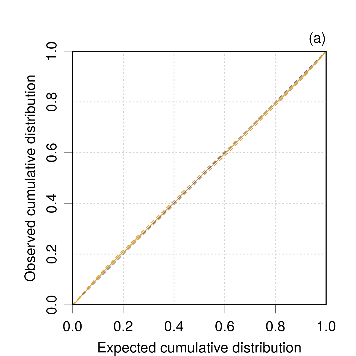
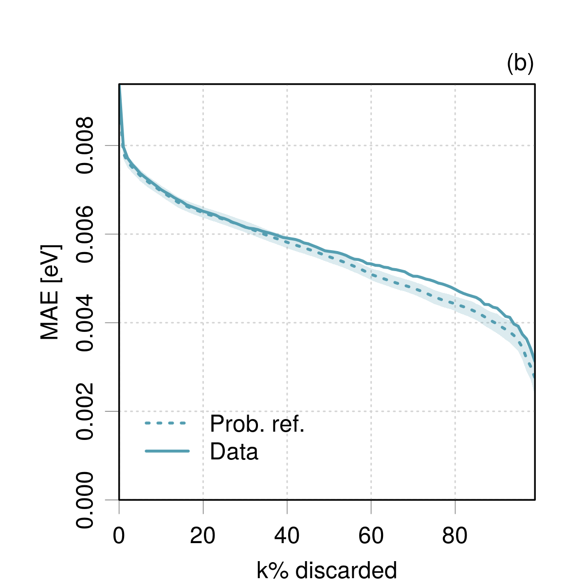
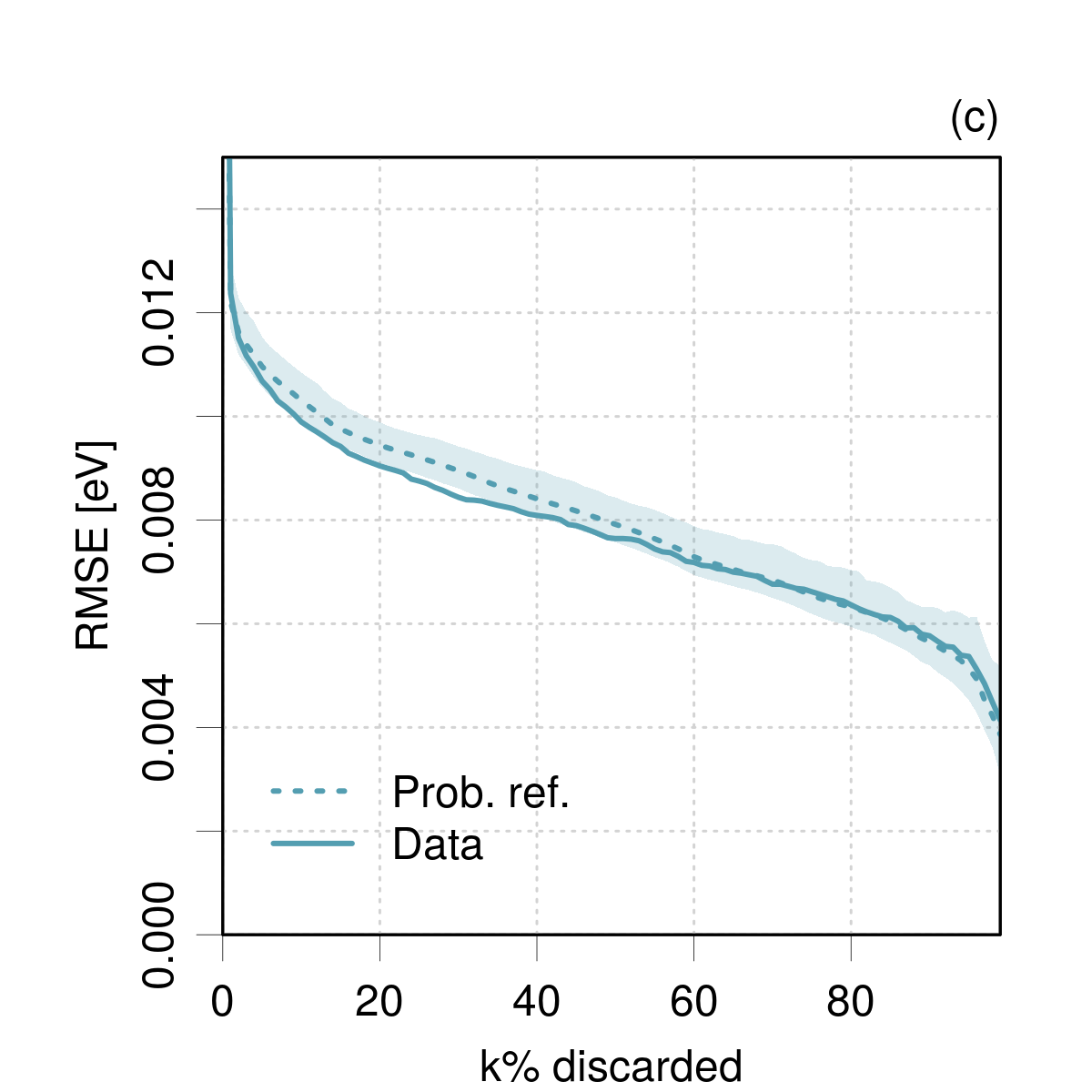
Figure 18: Case BUS2022: validation plots with a Student’s-$t_{\nu=4}$ generative distribution. (a) calibration curve; (b) MAE-based confidence curve; (c) RMSE-based confidence curve (the data curve has been truncated at 0.015 eV, but it decreases sharply from 0.031 eV).

IV.2.3 Conclusions

All diagnostics based on $E$ and $u_{E}$ conclude to a good calibration and consistency, notably if one accounts for a non-normal generative model ($t_{\nu=4}$). The main feature revealed by this reanalysis is the lack of adaptivity seen in the LZISD analysis in molecular mass space. It leads to a significant underestimation of the quality of predictions for the smaller molecules in the QM9 dataset. By contrast, the confidence curves indicate that the uncertainties can be used for active learning without a second thought.

IV.3 Case HU2022

These data were kindly collated and provided by Y. Hu to facilitate this reanalysis of the results presented in Figs. 3e and 3f of the paper by Hu et al.(Hu2022, ). These figures present plots of the errors on interatomic potentials for the QM9 dataset vs two distances: a distance in feature space, $X_{F}$ and a distance in latent space(Janet2019, ), $X_{L}$. Both distances have been calibrated to interval-based UQ metrics: the half-ranges of prediction intervals, $U_{F,P}$ and $U_{L,P}$ have been obtained for $P\in\{68,95\}$, by multiplication of the corresponding distances by probability-specific scaling factors optimized by conformal calibration to ensure average coverage. The percentage of points within the resulting intervals are reported in the original figures and show a successful average calibration in both cases. However, the distribution of points in these figures hints at different conditional calibration statistics for both metrics, which I propose to quantify in this reanalysis. The reader is referred to the original article for details on the dataset and ML-UQ methods.

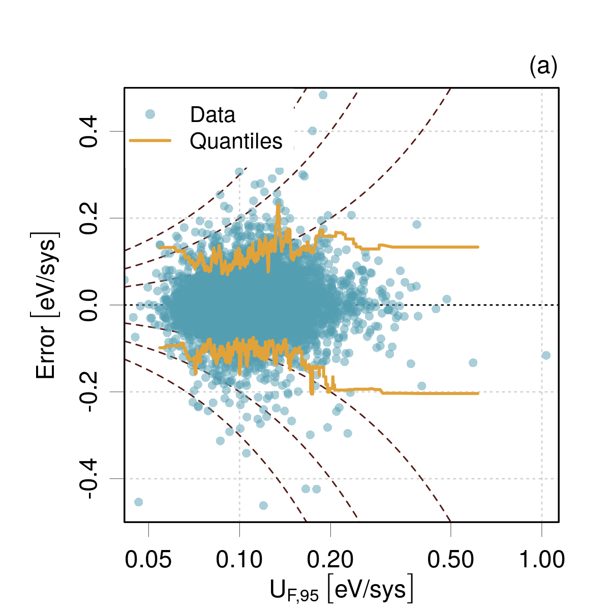
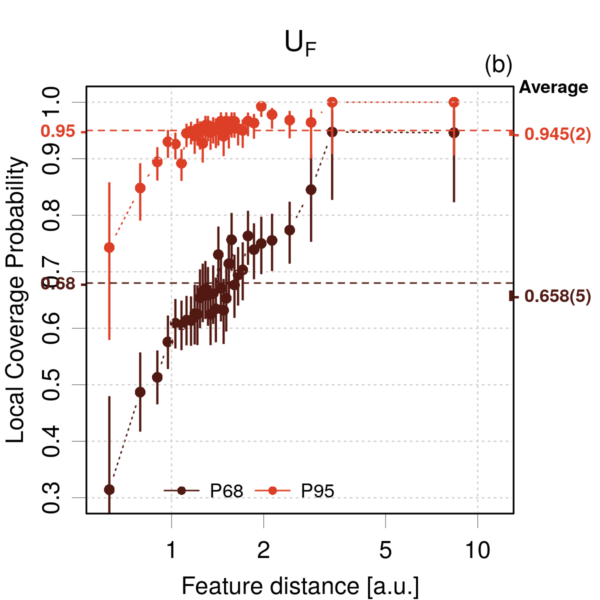
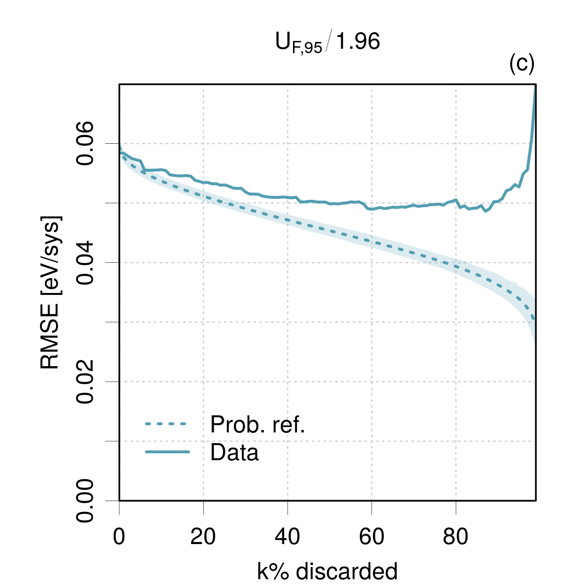
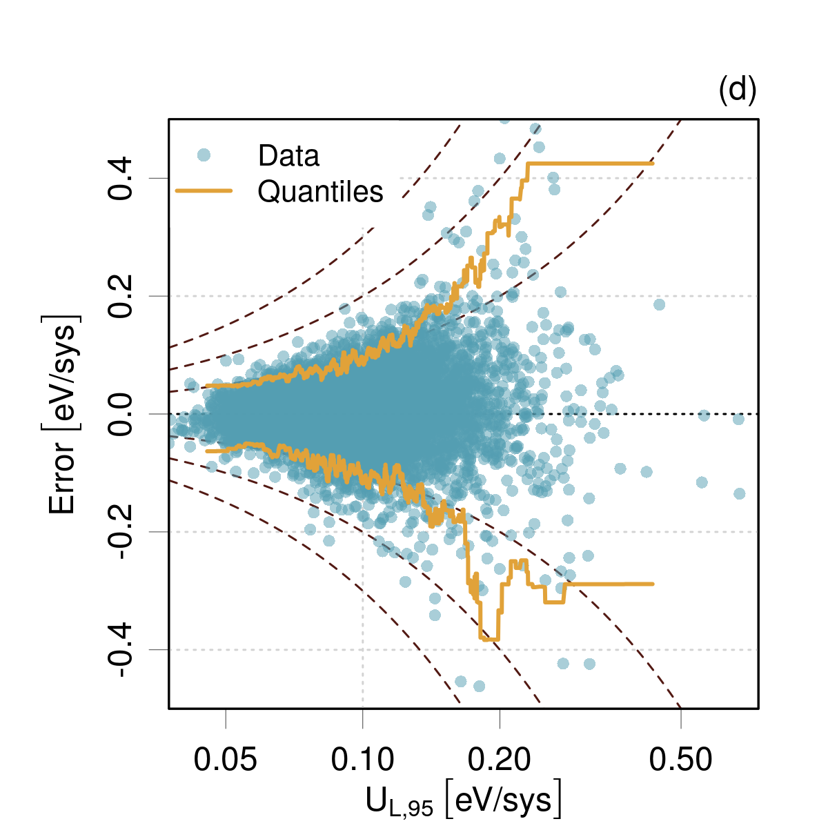
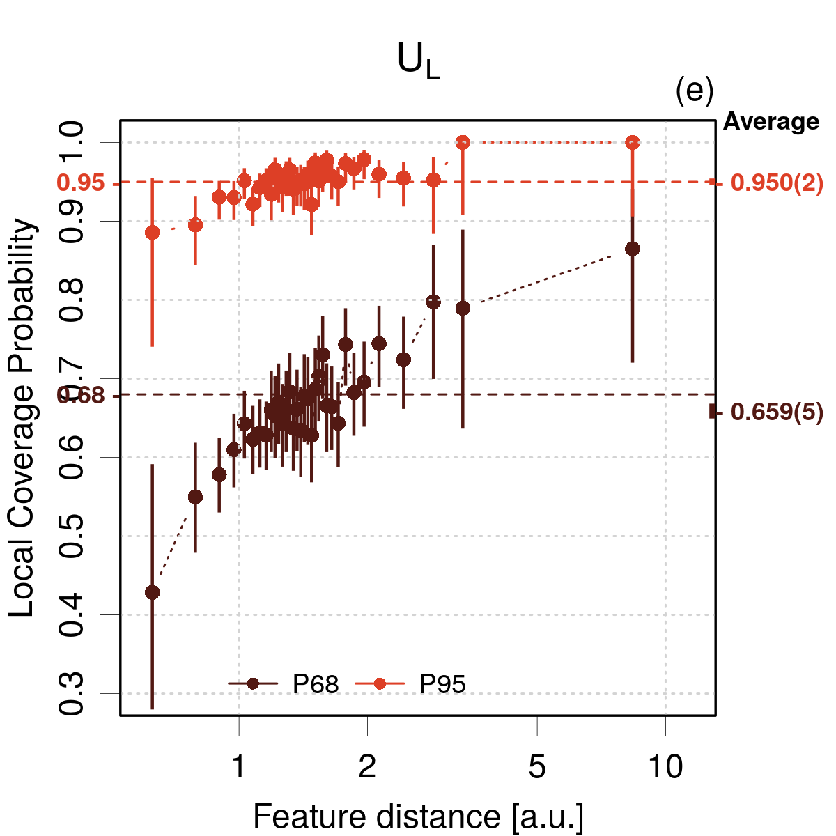
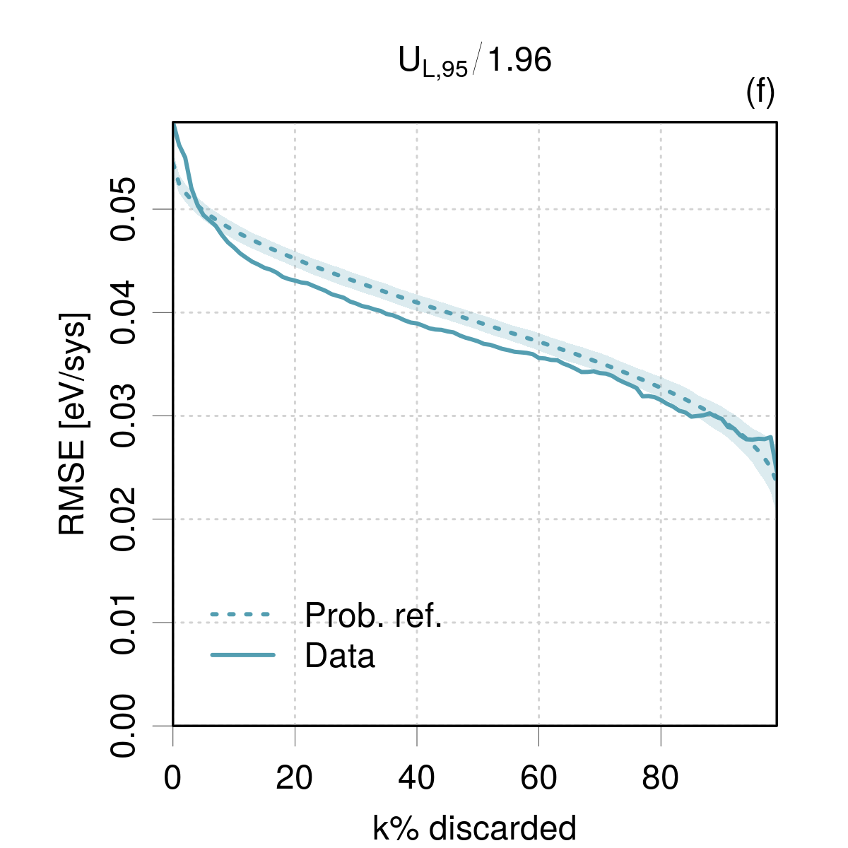
Figure 19: Case HU2022: (a) Error vs $U_{F,95}$; (b) LCP analysis for $U_{F,68}$ and $U_{F,95}$; (c) confidence curve for $U_{F,95}$; (d-f) idem with $U_{L,P}$. The LCP analysis uses an adaptive binning with a stating point of 20 bins).

A plot of the errors vs the expanded uncertainties at the 95 % level [Fig. 19(a,d)] confirms the features observed in the original figures: in this plot, the running quantiles should follow the $y=\pm x$ guide lines, which is not the case for $U_{F,95}$, while this seems to be much better for $U_{L,95}$, at least below 0.2 eV/sys.

To quantify this difference, the data are then analyzed with the LCP analysis in feature distance space [Fig. 19(b,e)]. As the data are conditioned over the feature distance, one is testing the adaptivity of the conformal calibration for individual predictions. Note that for $U_{F,95}$ the distances and uncertainties are proportional, and the adaptivity diagnostic is also a consistency diagnostic! A satisfying average coverage is reached in all cases, in agreement with the conclusions of the original article. However, the local coverage of $U_{L,P}$ is more homogeneous than for $U_{F,P}$ at both probability levels. The latter presents strong under- and over-coverage areas. The adaptivity of $U_{L,P}$ is not far from perfect at the 95 % level, except for the extreme bins, but is not good at the 68 % level.

It is also worthwhile to look at confidence curves[Fig. 19(c,f)]. The original article presents calibration curves which are very close to the identity line for both metrics. One can thus confidently transform the expanded uncertainties at the 95 % level to standard uncertainties using a normal distribution hypothesis. The resulting confidence curves display a much better behavior for $U_{L}$ than for $U_{F}$. For active learning, uncertainty built on latent distance looks therefore much more reliable than when built on feature distance. However, consistency is not perfect for $U_{L}$.

A simple scaling of the distance metrics by conformal inference results in a good average calibration, but it appears unable to ensure consistency/adaptivity. A better calibration would require to use conditional conformal calibration, which is reputed for its difficulty,(Vovk2012, ; Barber2019, ; Angelopoulos2021, ) and, as far as I know, has not yet been implemented in the ML-UQ context considered here.

V Conclusions

This article introduces a principled framework for the validation of UQ metrics. The studied examples target mostly machine learning in a materials science and chemistry context, but the applicability is more general. The concept of conditional calibration enables to define two aspects of local calibration: consistency, which assesses the reliability of UQ metrics across the range of uncertainty values, and adaptivity, which assesses the reliability of UQ metrics across the range of relevant input features.

The more or less standard UQ validation methods (calibration curves, reliability diagrams and confidence curves) were recast in the proposed framework, showing that they are not designed to test adaptivity. In consequence, adaptivity is presently a blind spot in the ML-UQ validation practice. It was shown on a few examples that consistency and adaptivity are scarcely reached by modern ML-UQ methods, and that a positive consistency diagnostic does not augur of a positive adaptivity diagnostic. Both aspects of local calibration should be tested.

Let us summarize the main points arising from this study.

Consistency testing.

Beside the exploratory “$E$ vs $u_{E}$” plots, three validation methods have some pertinence to test consistency of variance-based UQ metrics:

• Error vs Uncertainty plots offer a very informative preliminary analysis, devoid of any artifacts due to a binning strategy or the choice of a generative distribution. However, they do not enable to conclude positively on consistency, which requires more quantitative diagnostics.

• Reliability diagrams and LZV/LZISD analysis are direct implementation of the conditional calibration tests. It was shown that the LZV/LZISD analysis offers a visually more discriminant approach, along with a direct quantification of possible uncertainty misestimations. Both methods are sensitive to the choice of a binning scheme, and an adaptive binning scheme is proposed to compensate for the drawbacks of equal-counts or equal-width binning strategies.

• The RMSE-based confidence curve is not designed to check consistency, but, augmented with a probabilistic reference, it offers an interesting approach, combining two diagnostics: the eligibility of the UQ method for a reliable active learning and the consistency of the dataset. Moreover, it is less dependent on a binning strategy than the reliability diagrams or LZV/LZISD analysis. An inconvenience is the dependence of the statistical validation reference curve (more precisely its confidence band) on the choice of a generative distribution.

I have also shown that conditional calibration curves could be considered to assess consistency. As for confidence curves, their disadvantage for variance-based UQ metrics is the difficulty to discern between a lack of consistency or a bad choice of generative distribution hypothesis. For the latter point, care has to be taken in particular for UQ metrics based on small ensembles.

I would then recommend the Error vs Uncertainty plot, the LZISD analysis and the RMSE-based confidence curve with its probabilistic reference as complementary diagnostics for the consistency of variance-based UQ metrics.

For interval-based UQ metrics the LCP analysis seems to be the best choice, as it implements directly the conditional calibration test. Calibration curves have been shown to have possibly ambiguous diagnostics, which can be improved by using conditional calibration curves. In order to avoid undue hypotheses about an error generative distribution, interval-based validation methods should be reserved to interval-based UQ metrics.

Adaptivity testing.

Adaptation of the standard methods to test conditional calibration over some input feature is not ideal but feasible, and one could envision conditional reliability diagrams, conditional calibration curves, and even conditional confidence curves. This approach requires large validation datasets and leads to complex graphs that are not easily legible. In addition to the Z vs Input feature plots, I would then recommend the LZISD analysis and the LCP analysis as general tools to test adaptivity of variance- and interval-based UQ metrics, respectively.

It was also noted that using the predicted values $V$ as a conditioning variable to test adaptivity is not without risks, as it might produce spurious features that complicate the diagnostic. This should probably be generalized to any property that is susceptible to be strongly correlated with the errors. Further studies are required to clear this up.

I hope that the proposed framework, articulated around conditional calibration, will help ML-UQ researchers to approach UQ validation with a renewed interest. Up to now, ML-UQ validation studies were mainly focused on conditional calibration with respect to uncertainty, i.e. consistency. There is a strong need that adaptivity be also considered, notably for final users who expect UQ metrics to be reliable throughout input features space.

Author Declarations

Conflict of Interest

The authors have no conflicts to disclose.

Code and data availability

The code and data to reproduce the results of this article are available at https://github.com/ppernot/2023_Primer/releases/tag/v1.0 and at Zenodo (https://doi.org/10.5281/zenodo.7731669). The R,(RTeam2019, ) ErrViewLib package implements the validation functions used in the present study, under version ErrViewLib-v1.7.0 (https://github.com/ppernot/ErrViewLib/releases/tag/v1.7.0), also available at Zenodo (https://doi.org/10.5281/zenodo.7729100). The UncVal graphical interface to explore the main UQ validation methods provided by ErrViewLib is also freely available (https://github.com/ppernot/UncVal).

Appendices

Appendix A Using the predicted value to test adaptivity

A posteriori validation of adaptivity on datasets that do not contain input features $X$ might still be attempted by using the predicted values $V$ as proxy. Conditional calibration on $V$ is not necessarily identical to conditional calibration on $X$, but it might still provide useful diagnostics.

Application of “$Z$ vs $V$” plots to the synthetic datasets is presented in Fig.A1(a-f). Z-score values in Case A are globally well distributed (horizontal running quantiles around $\pm 2$, but present an anomaly at small $V$ values. This can be traced back to the correlation of $V$ with $E$ ($E=R-V$), most visible when $R$ is nearly constant at the bottom of the parabolic model used to generate the data. This warns us that conditioning on $V$ might produce some aberrant features, which are not diagnostic of poor adaptivity. The same artifact can be observed in Cases D, E and F. For Case E, the excessive dispersion of points, with $|Z|$ values above 5, points to a non-normal distribution, but this should not be a valid reason to reject adaptivity: a more quantitative analysis is mandatory. By contrast, the absence of adaptivity is readily visible for cases B, C, and D : cases B and C present heterogeneous distributions along $V$, while Case D has $Z$ values mostly contained between -1 and 1, pointing to an homogeneous overestimation of uncertainties. Case F is similar to Case A.

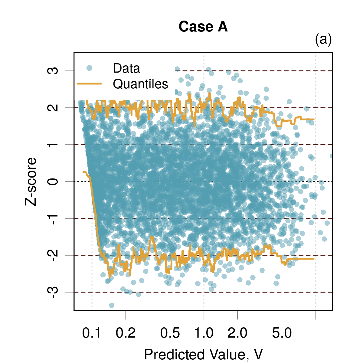
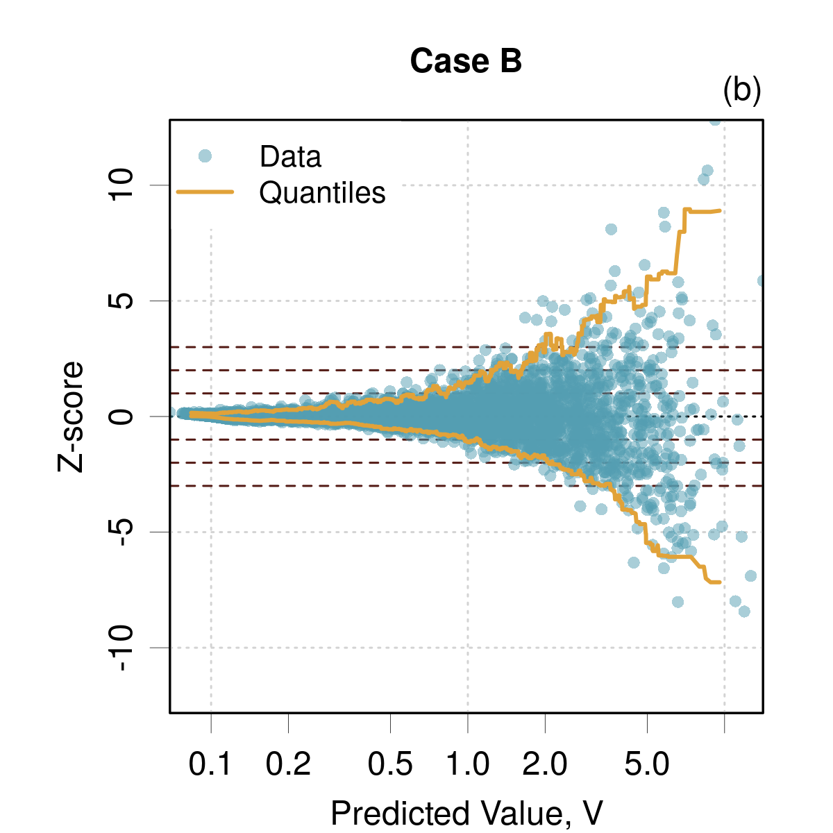
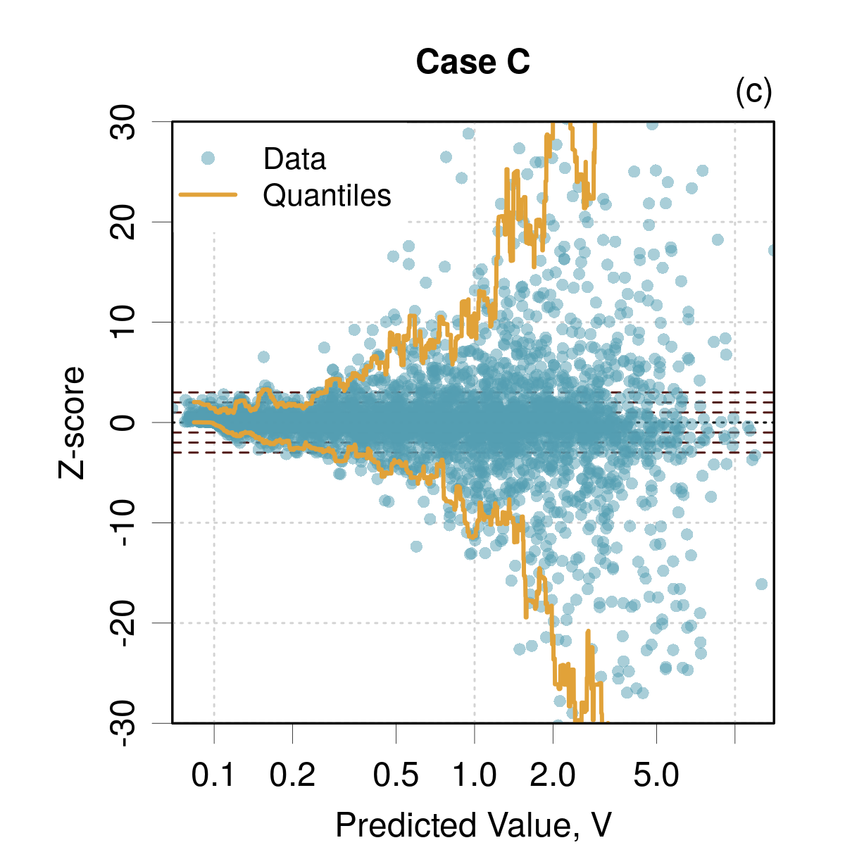
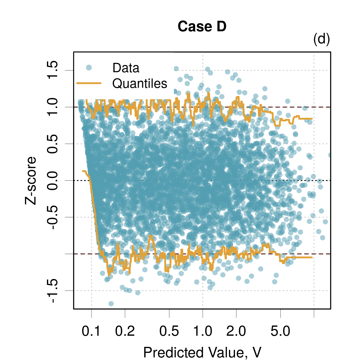
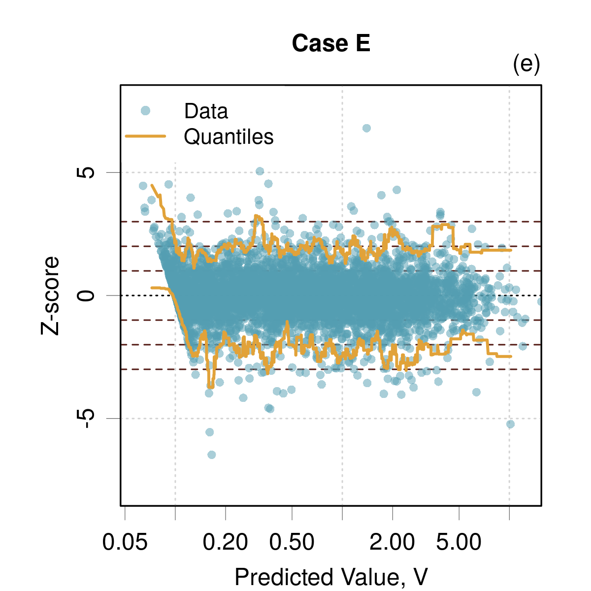
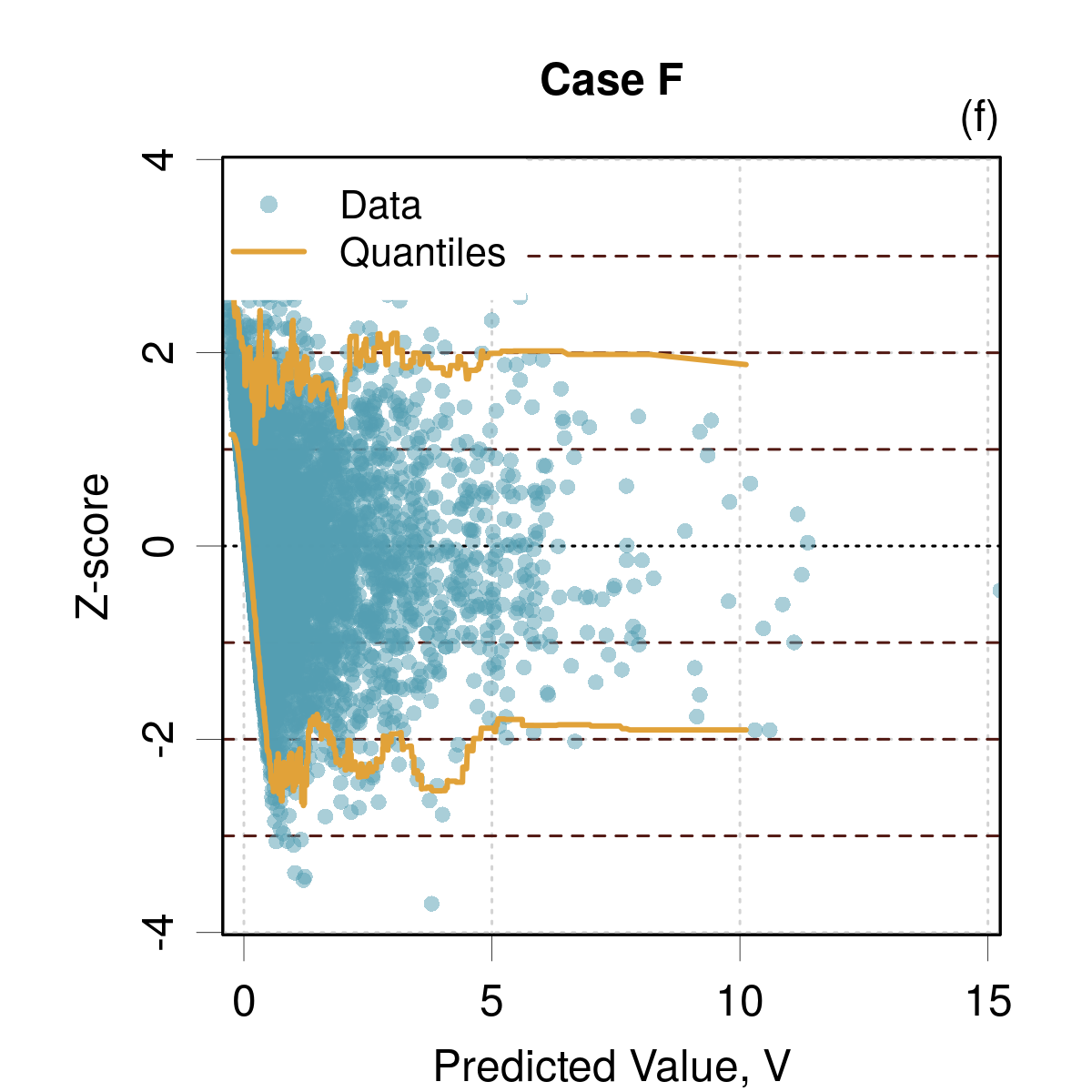
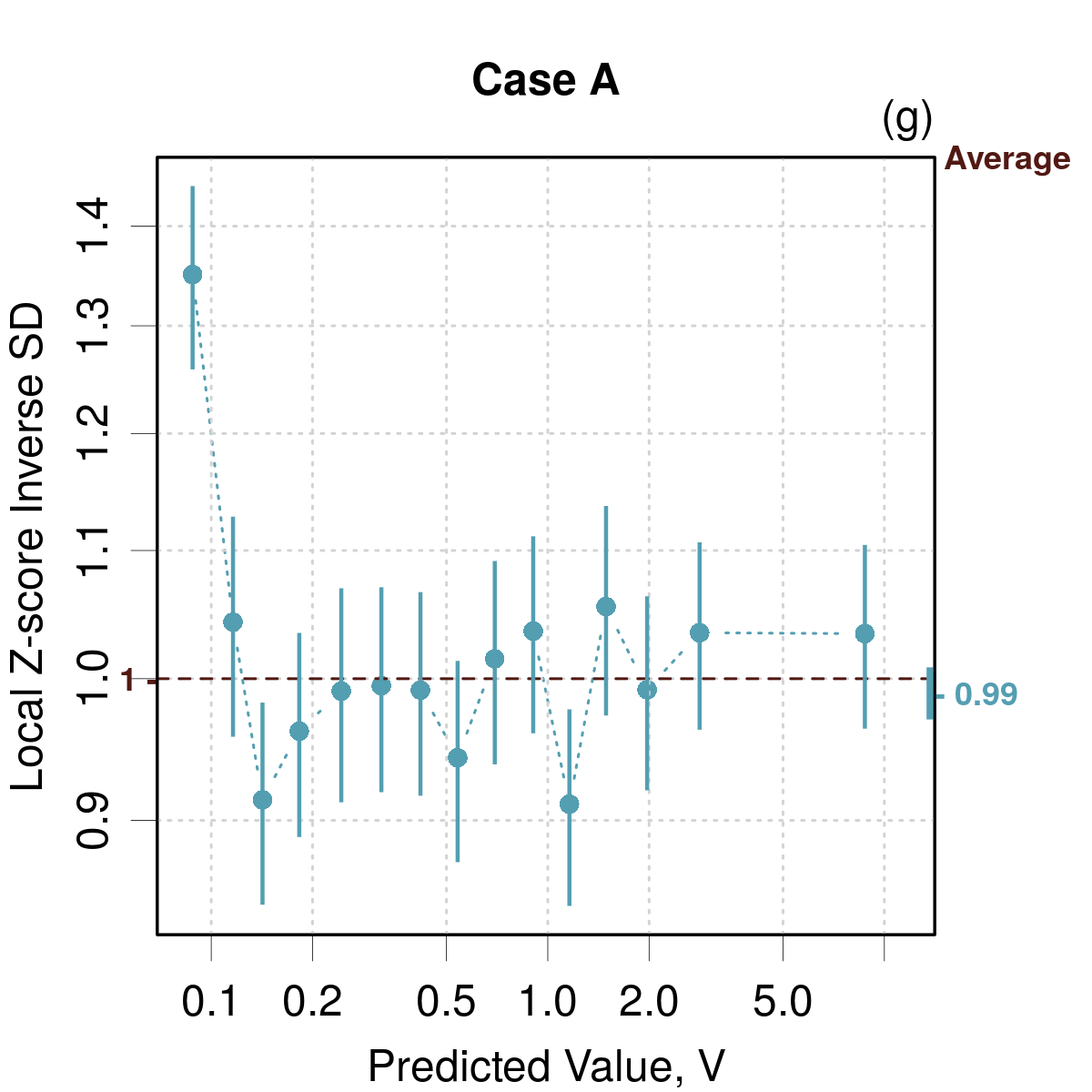
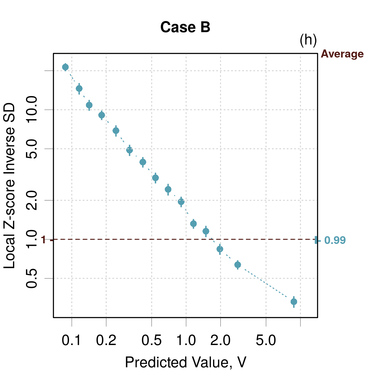
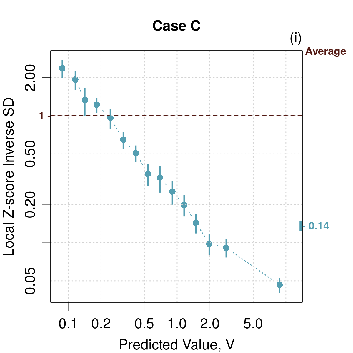
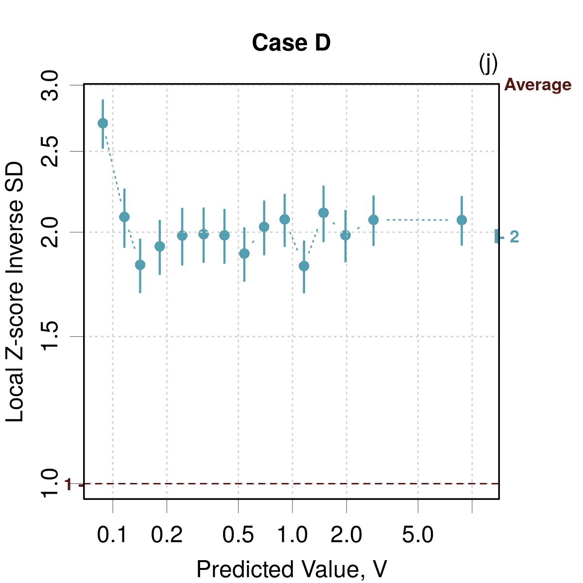
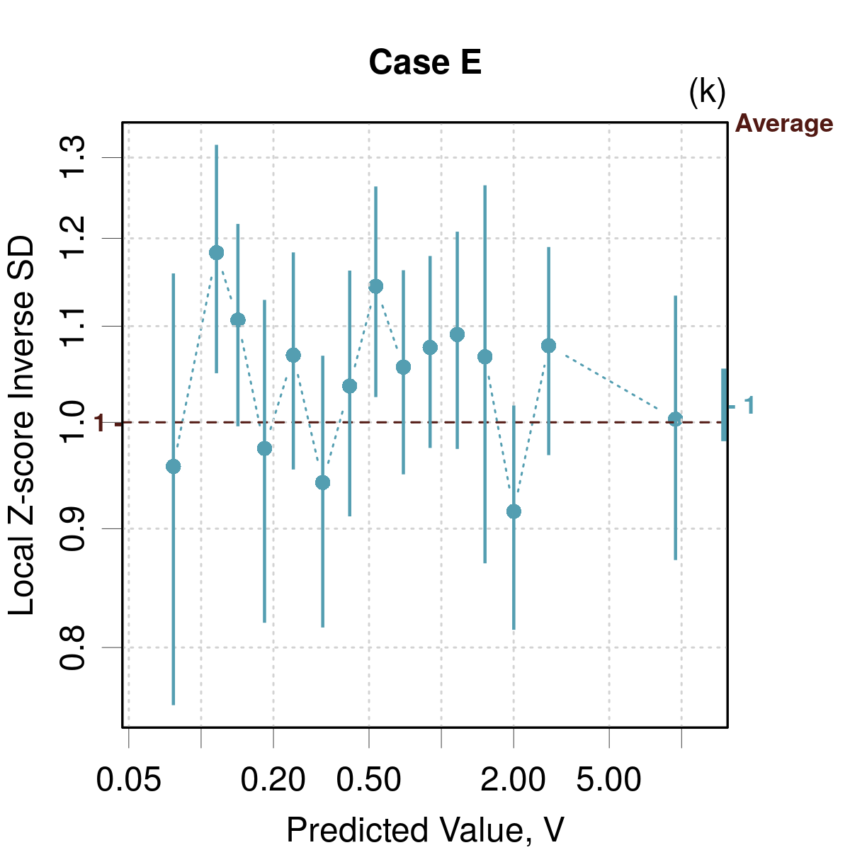
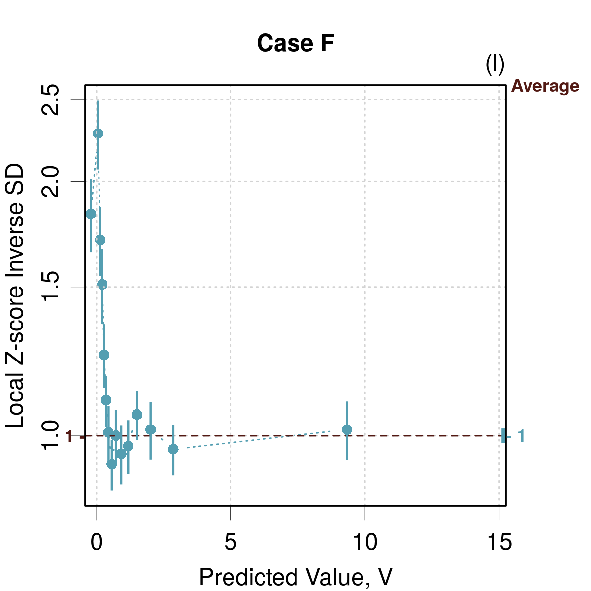
Figure A1: Validation of adaptivity vs predicted values $V$ for synthetic datasets: (a-f) ”$Z$ vs $V$” plots; (g-l) LZISD analysis.

The translation of these observations to the LZISD analysis is presented in Fig. A1(g-l). The artifact appears as local deviations of the LZISD values, while the intrinsic non-adaptivity of Cases B and C is more global. Similar observations can be made on the conditional calibration curves and LCP analyses (not shown).

This shows that using $V$ as a substitute for $X$ to test adaptivity might lead to ambiguous conclusions when local anomalies are observed. However, global anomalies are certainly diagnostic of a lack of adaptivity of the tested UQ metric.

Appendix B Impact of the binning strategy

To implement the LZV analysis, the default binning strategy is based on intervals with (nearly) equal populations.(Pernot2022a, ) This ensures equal testing power in all intervals, but might result in intervals with very different ranges. This is also often the strategy chosen for reliability diagrams.(Scalia2020, ) However, some authors prefer to use bins with similar widths,(Palmer2022, ) a strategy which faces two problems: bins with insufficient population to derive reliable confidence intervals, and bins containing a large part of the total sample for uncertainty distributions with large tails.

These problems were addressed by Palmer et al.(Palmer2022, ) by labeling the bins with less than 30 points as unreliable and by altering the width of bins in the peak area to ensure that the lowest 90% of the values were spread across at least five bins (assuming that uncertainty distributions can only have a heavy upper tail). The use of this strategy leads to very regular reliability diagrams with deviant points mostly in the upper range of uncertainty.

I present here an alternative binning strategy, considering that for a positive variable such as uncertainty, a log-transform might be an efficient way to reduce the skewness of the distribution causing the accumulation problem in a few bins. Starting from a regular grid in log space ($n$ bins), the problem of small counts is solved by merging adjacent bins with insufficient populations, while the problem of excessively large counts is solved by splitting bins having more than $M/n$ points ($M$ is the dataset size). Both operations are iterated until the bins population conforms with the chosen limits (the lower limit is set to 30).

Two examples below, taken from Palmer et al.(Palmer2022, ) (see Sect. IV.1), show that this adaptive strategy is more efficient to reveal consistency problems. The Diffusion/LR and Perovskite/GPR_Bayesian datasets were analyzed by reliability diagrams and LZISD analysis for increasing number of bins (10, 20 and 40) for the equal-counts bins and adaptive strategies. The reliability diagrams have also to be compared with those of the original article, based on 15 equal-width bins.

Let us consider first the Diffusion/LR case. For both types of analysis, the counts-based binning [Fig. A2(a-f)] needs at least 20 bins to reveal an overestimation problem for the largest uncertainties, with a stronger effect for 40 bins. The averaging effect in large bins ($n=10$) would lend us to believe that calibration is good in this area, whereas using four times smaller bins reveals uncertainty in excess by a factor two around 2 eV.

By using the new adaptive strategy [Fig. A2(g-l)], the problem is apparent for all the specified numbers of bins. In fact, for a starting point of 10 bins, the merge/split strategy converges to 20 bins, for 20 bins, one gets 30 and for 40 bins 47. The first case provides a good binning without the useless details that arise from the higher bin numbers.

For this dataset, one clearly has consistency problems with under- and over-estimation for uncertainties larger than 0.5. These defects compensate each other and are not detected when using large bins. This problem is also apparent in the original article [Figure 2(d)], albeit for a series of bins with populations below the 30 limit. Aggregating these bins enables to conclude that the effect is statistically significant.

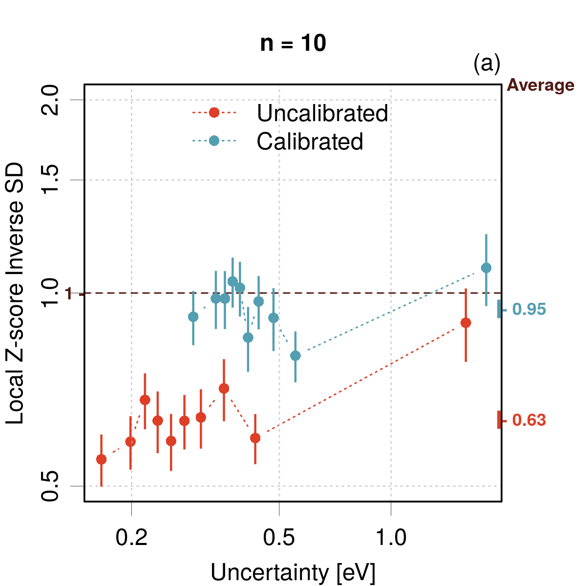
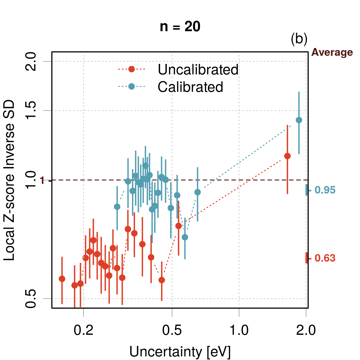
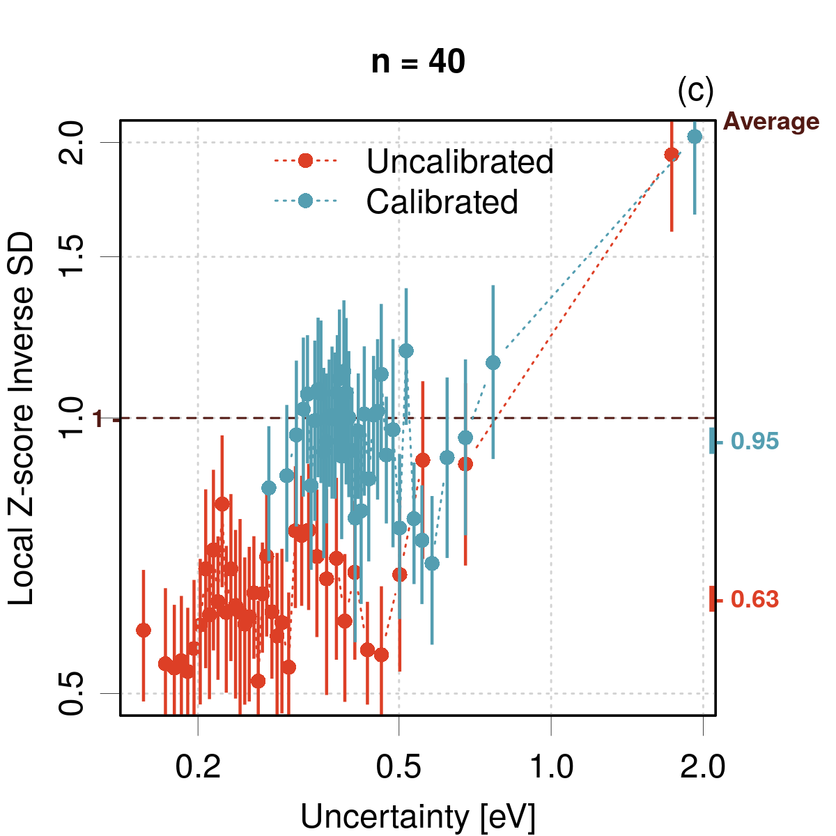
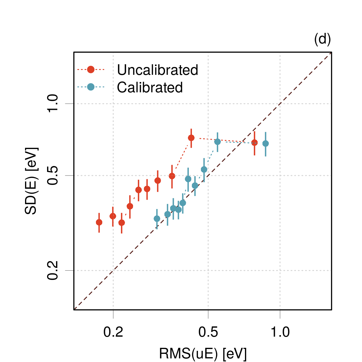
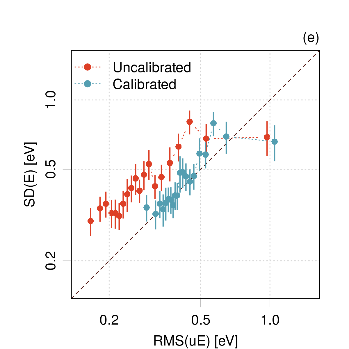
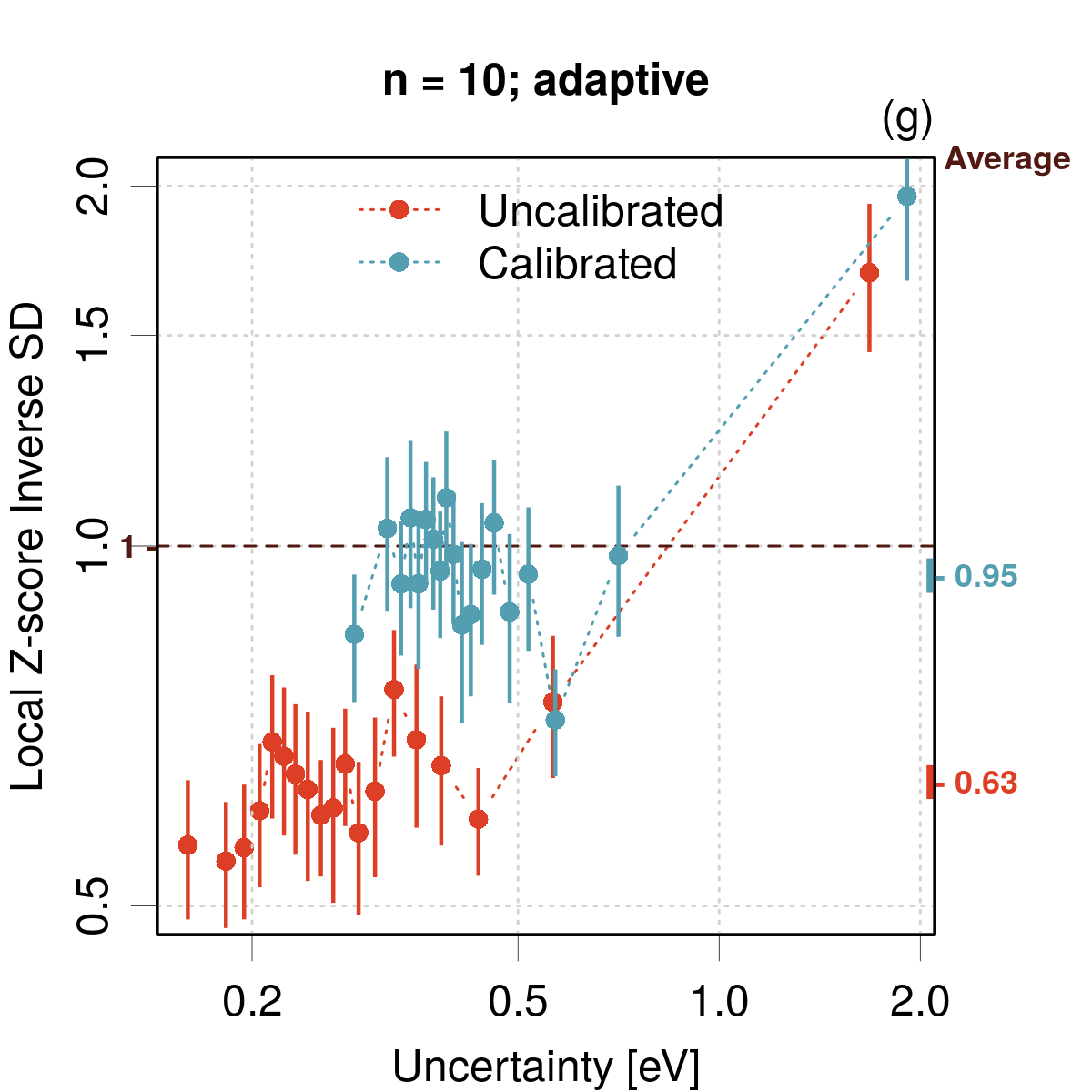
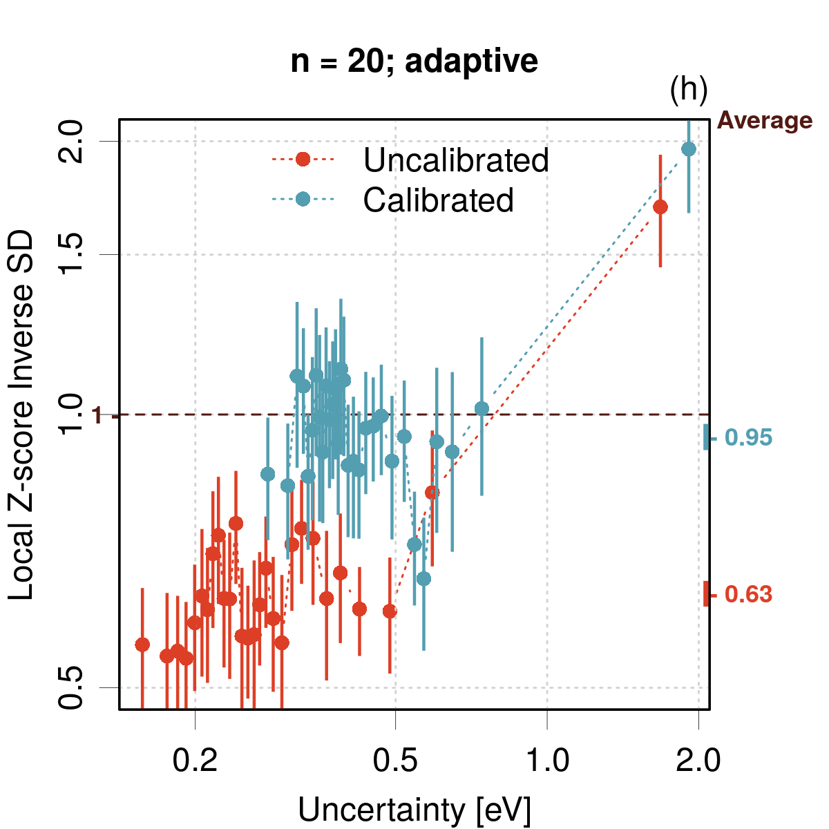
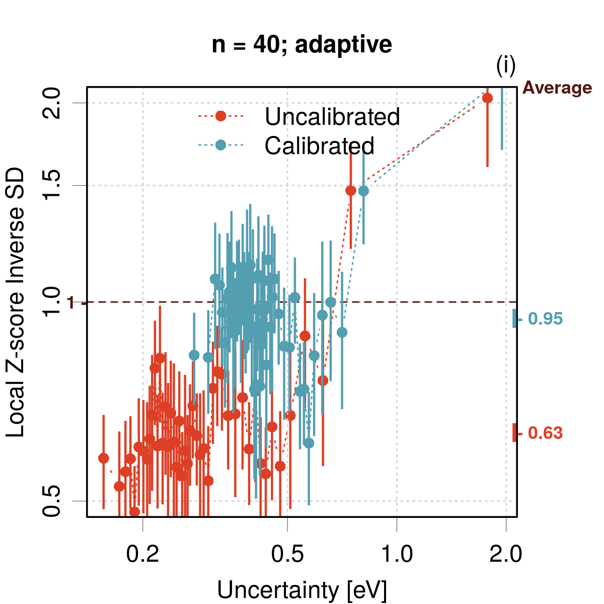
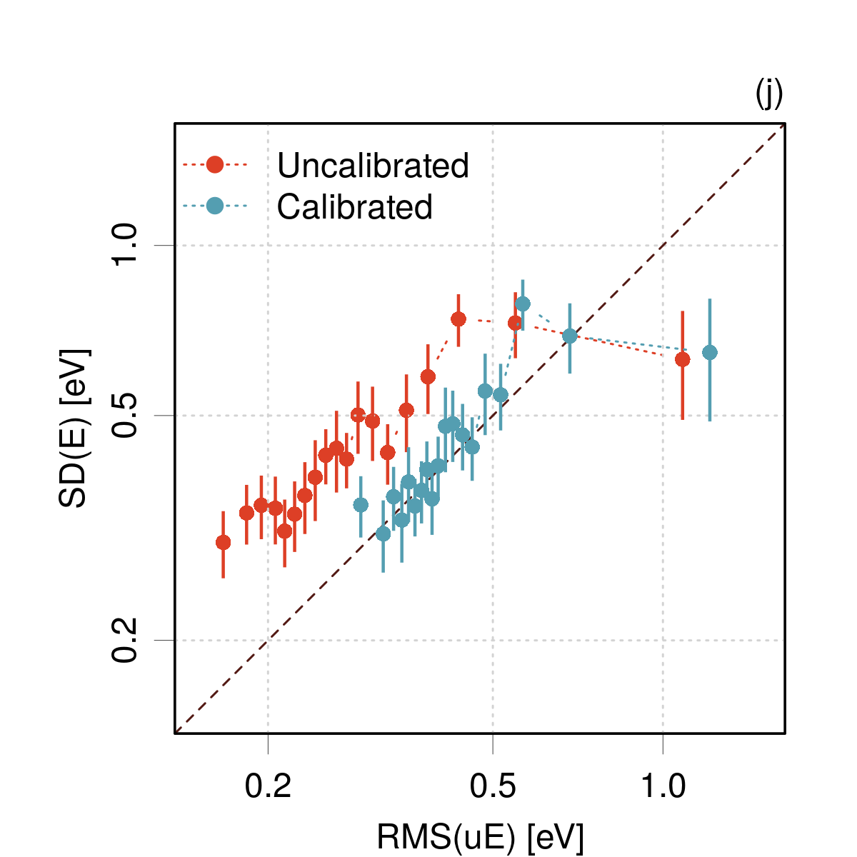
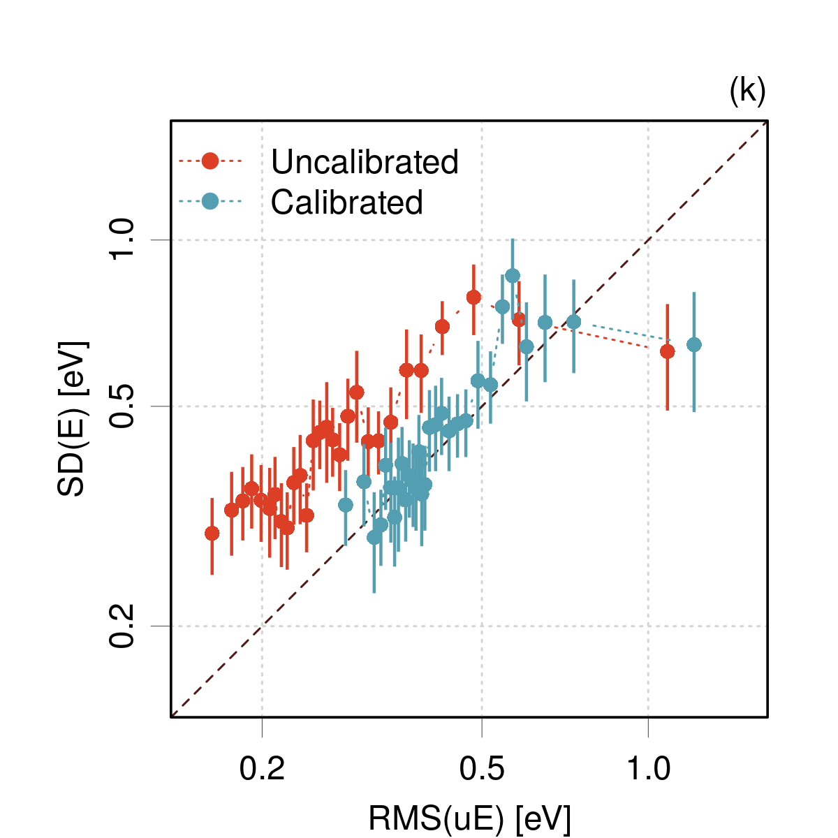
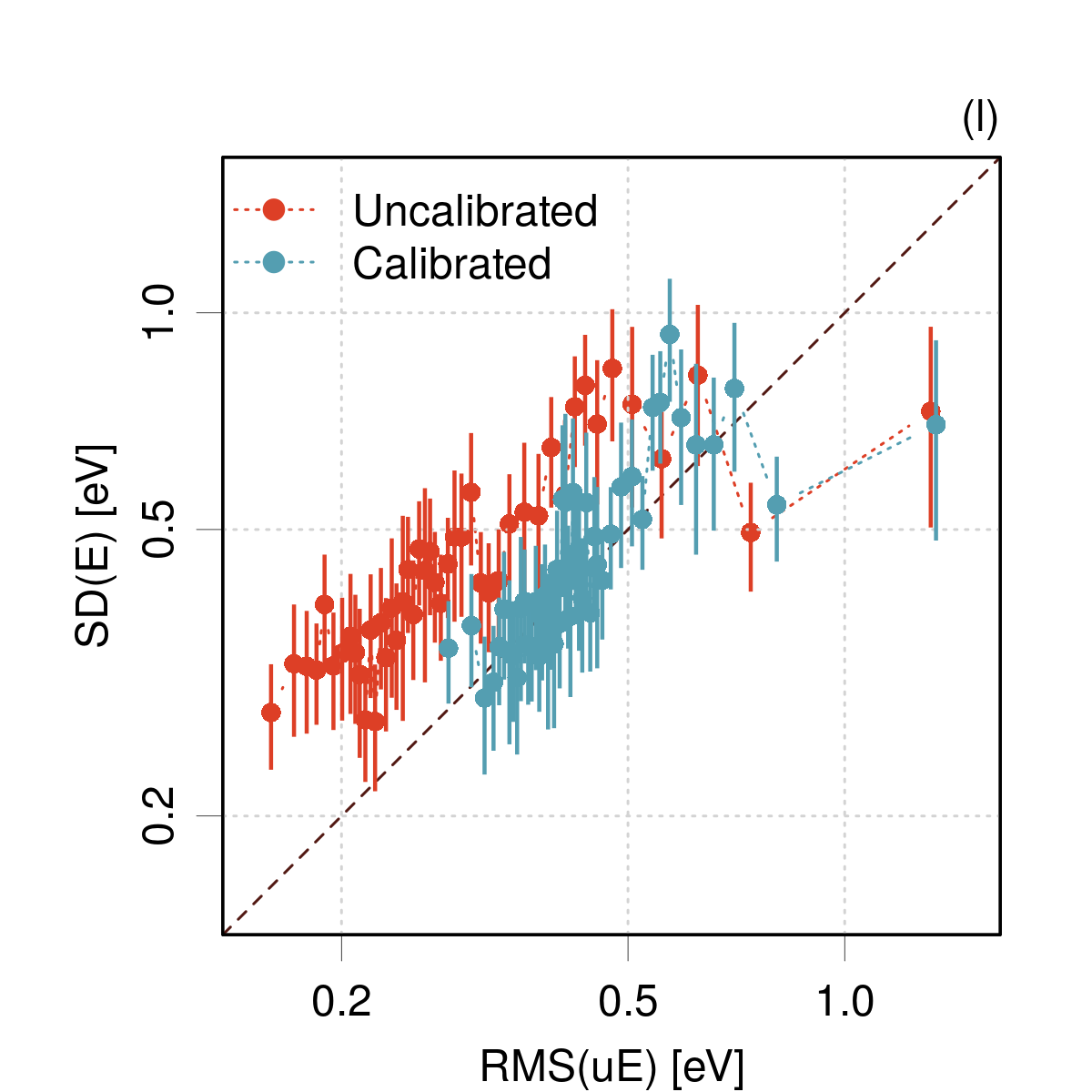
Figure A2: Case PAL2022/Diffusion_LR. Impact of the number of bins on LZISD analysis and reliability diagrams: (a-f) bins with equal populations; (g-l) adaptive strategy.

The Perovskite/GPR_Bayesian case is shown in Fig. A3. As in the previous example, the counts-based binning needs more than 20 bins to display a problem at small uncertainties, in both LZV and RD analyses [Fig. A3(a-f)]. The LZV analysis indicates a strong overestimation of the uncertainties around 0.01 eV, the reliability diagram showing that the corresponding errors have a standard deviation of about 1E-8, which would certainly deserve a closer inspection. The adaptive analysis needs 20 initial bins (30 after adaptation) to reveal the problem [Fig. A3(g-l)]. This “data nugget” is undetected by the linear equal-width binning of the original study (see Figure 38 of the Supplementary Information to Palmer et al.(Palmer2022, )).

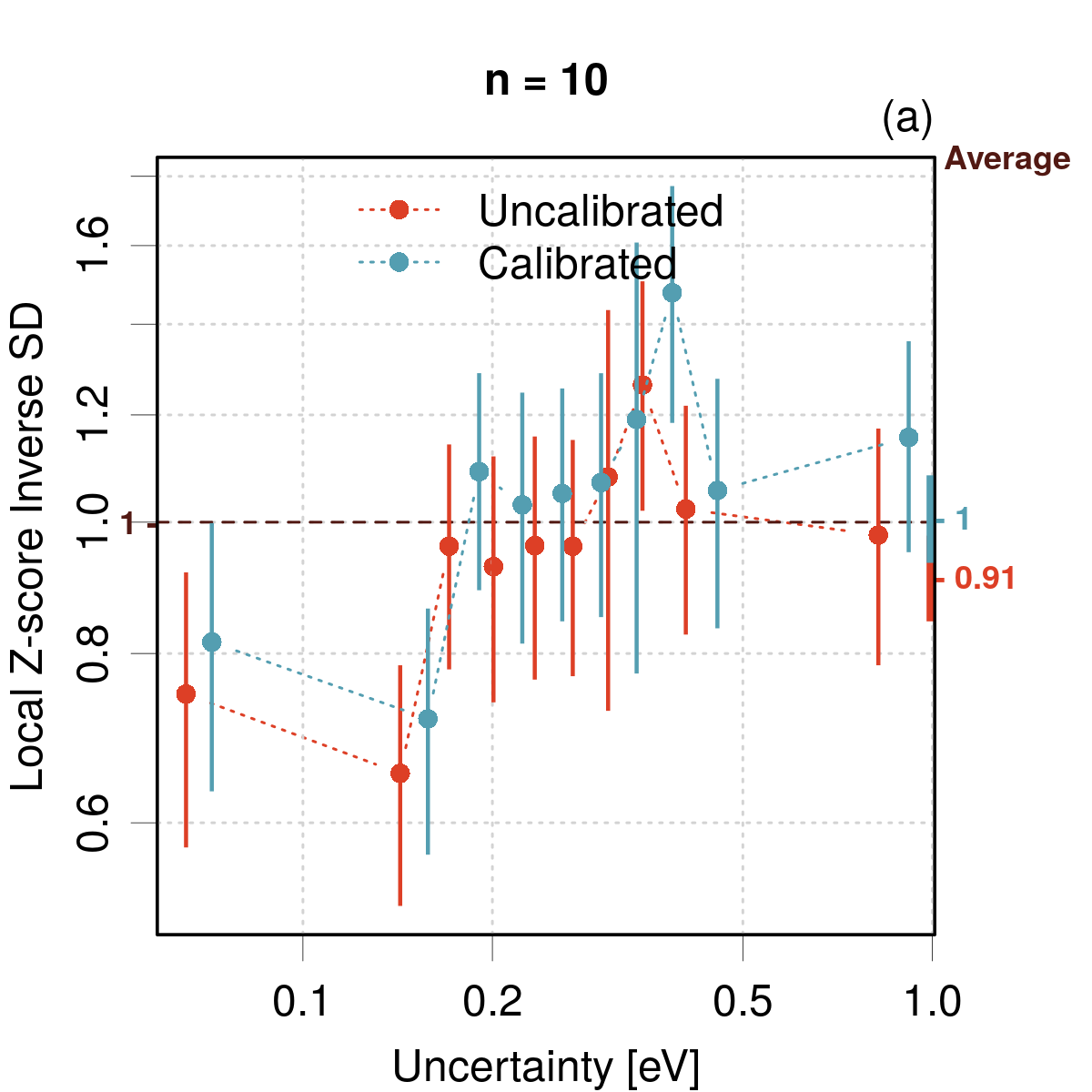
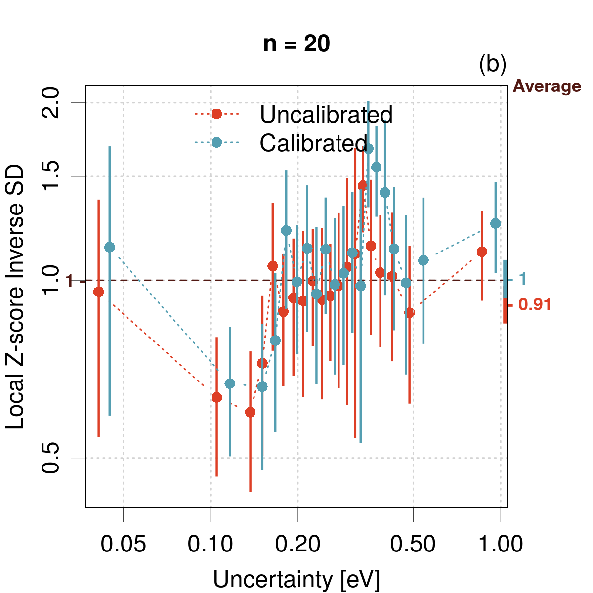
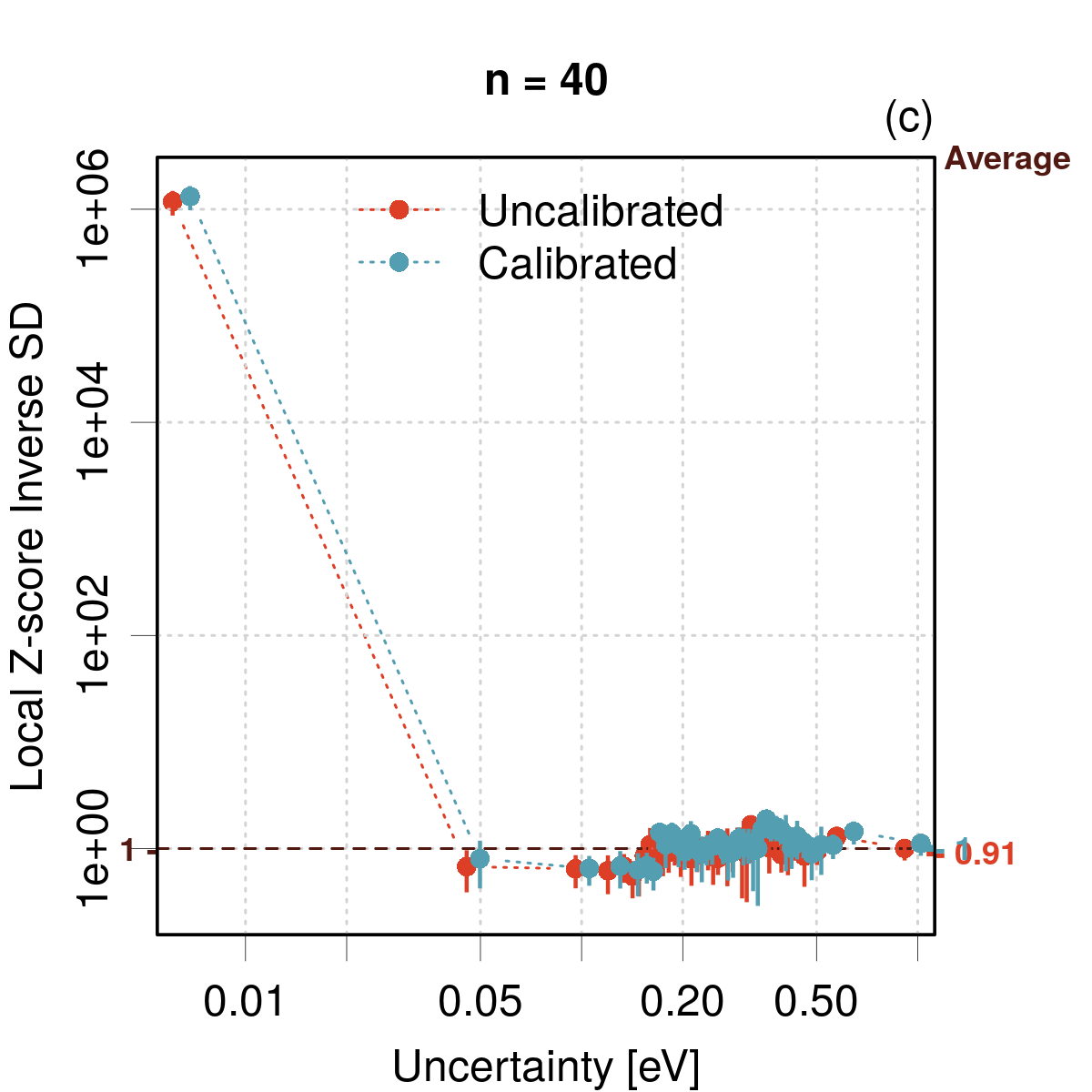
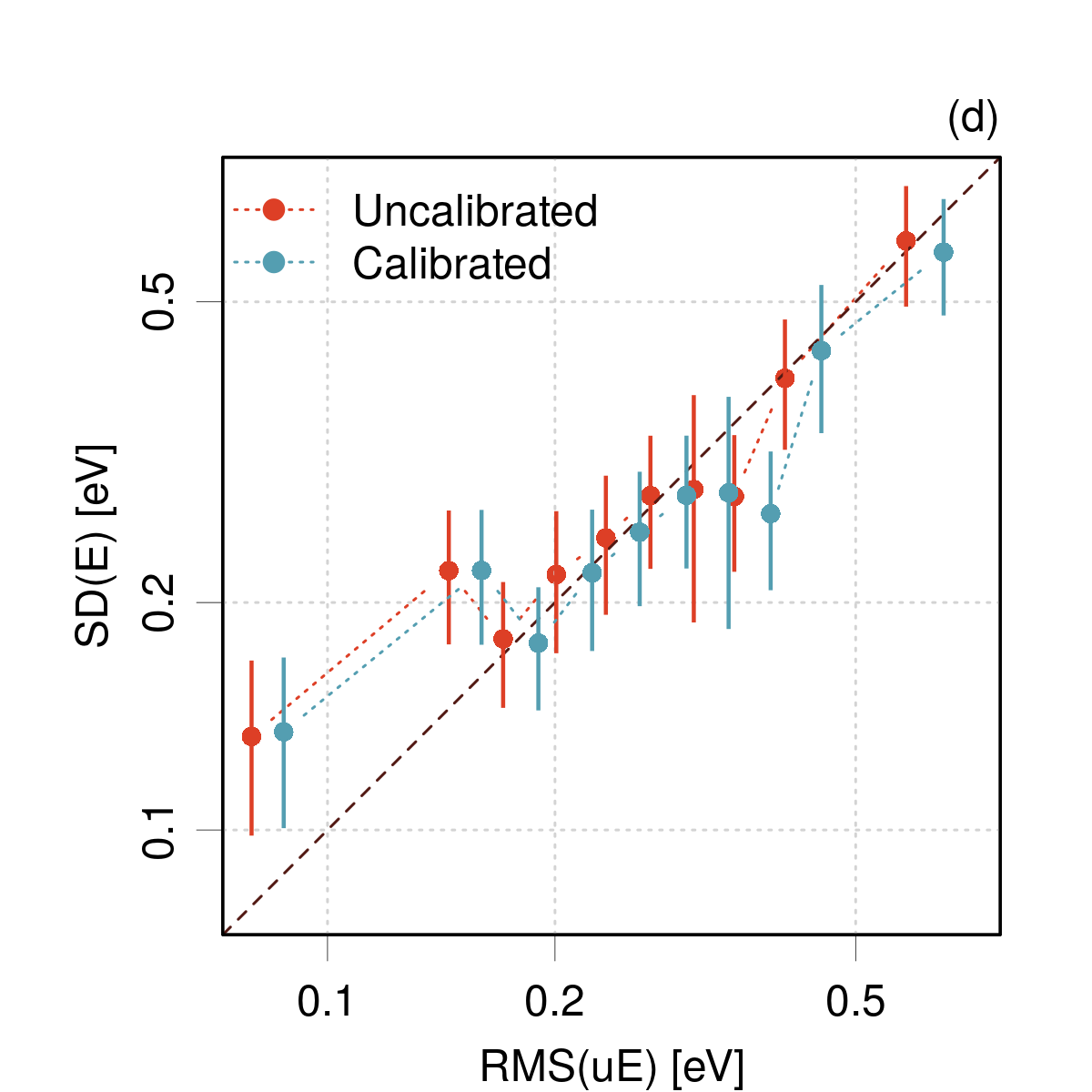
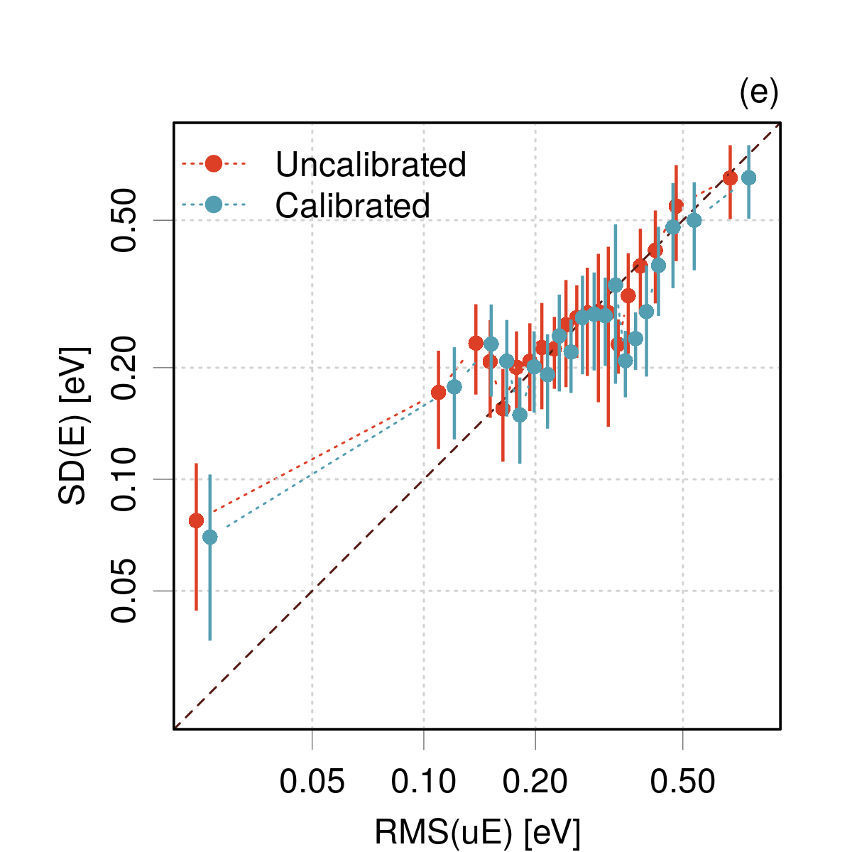
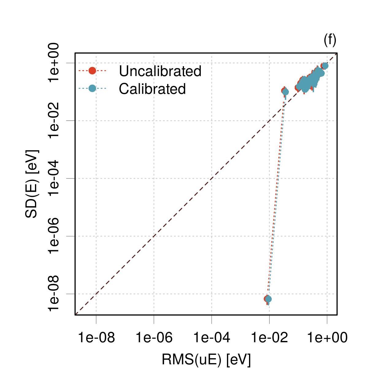
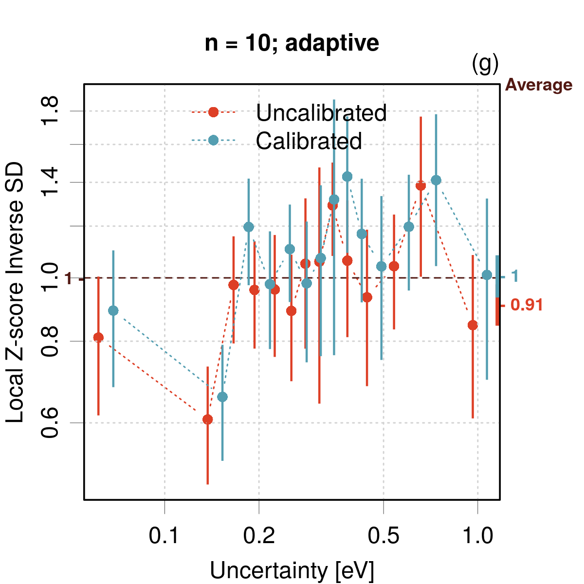
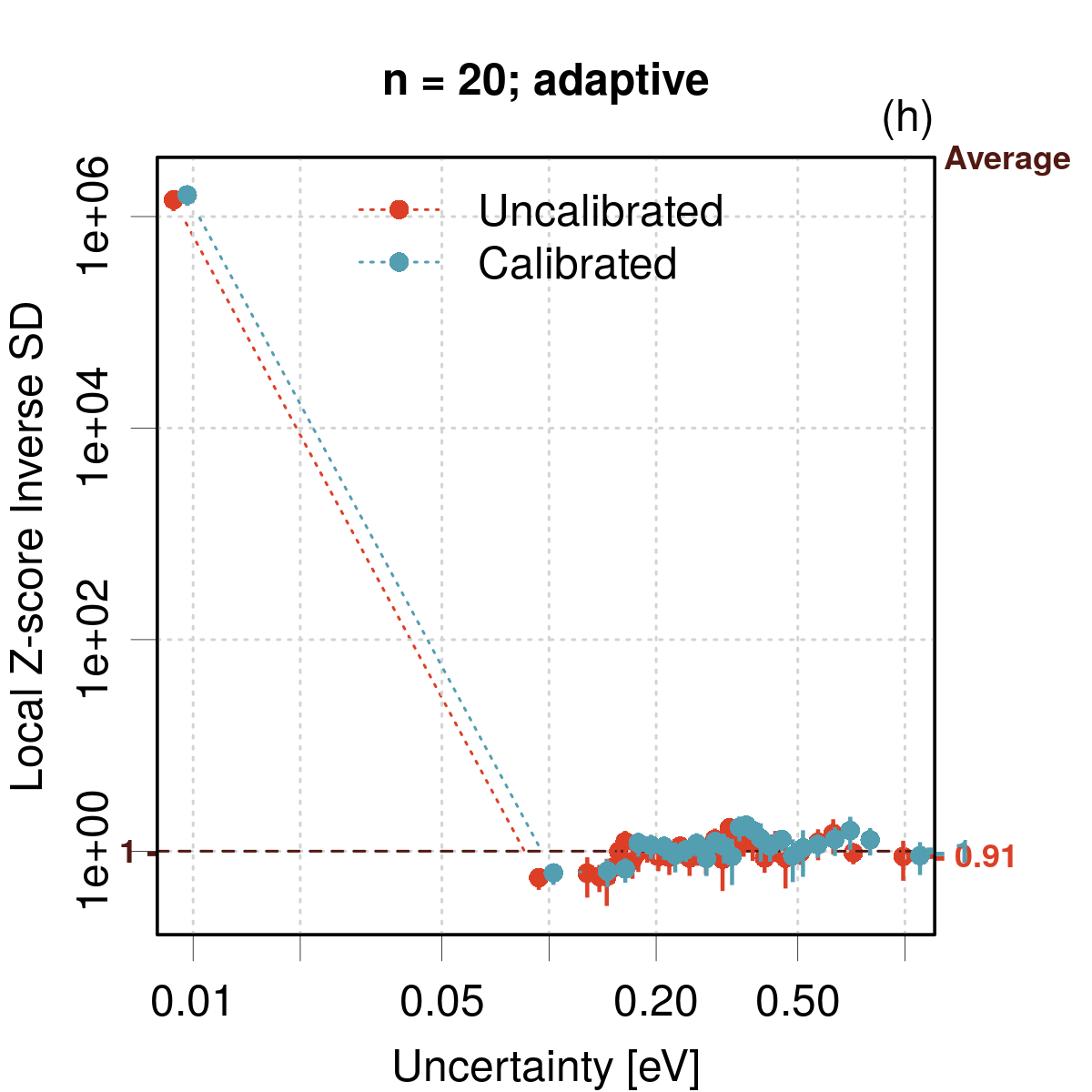
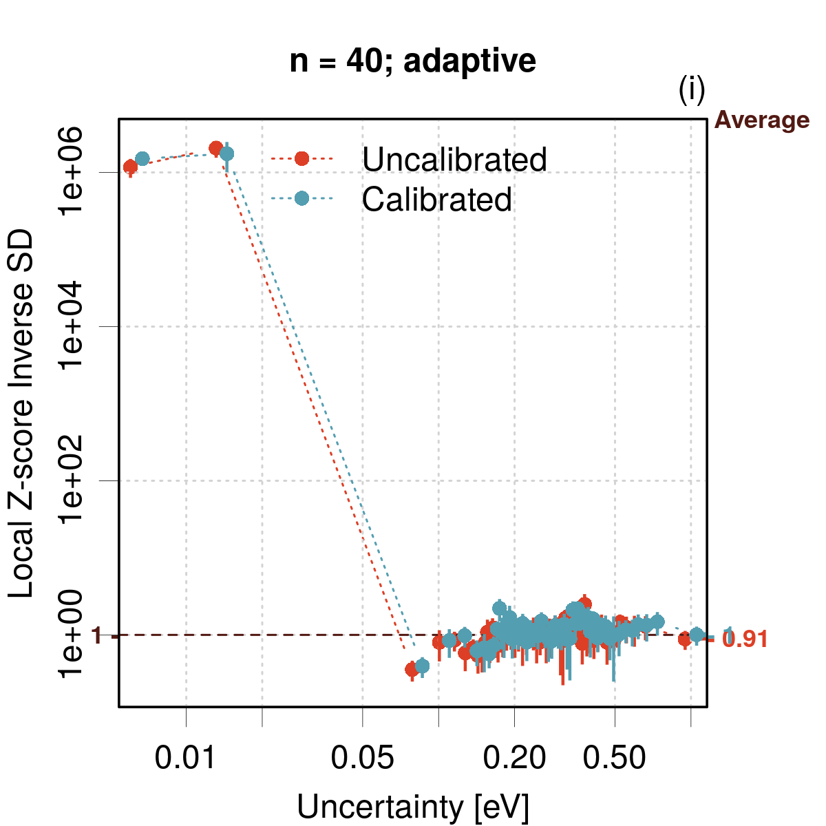
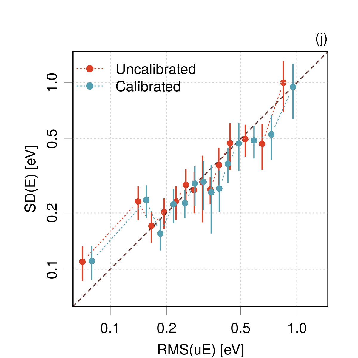
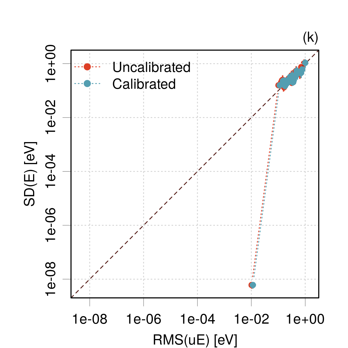
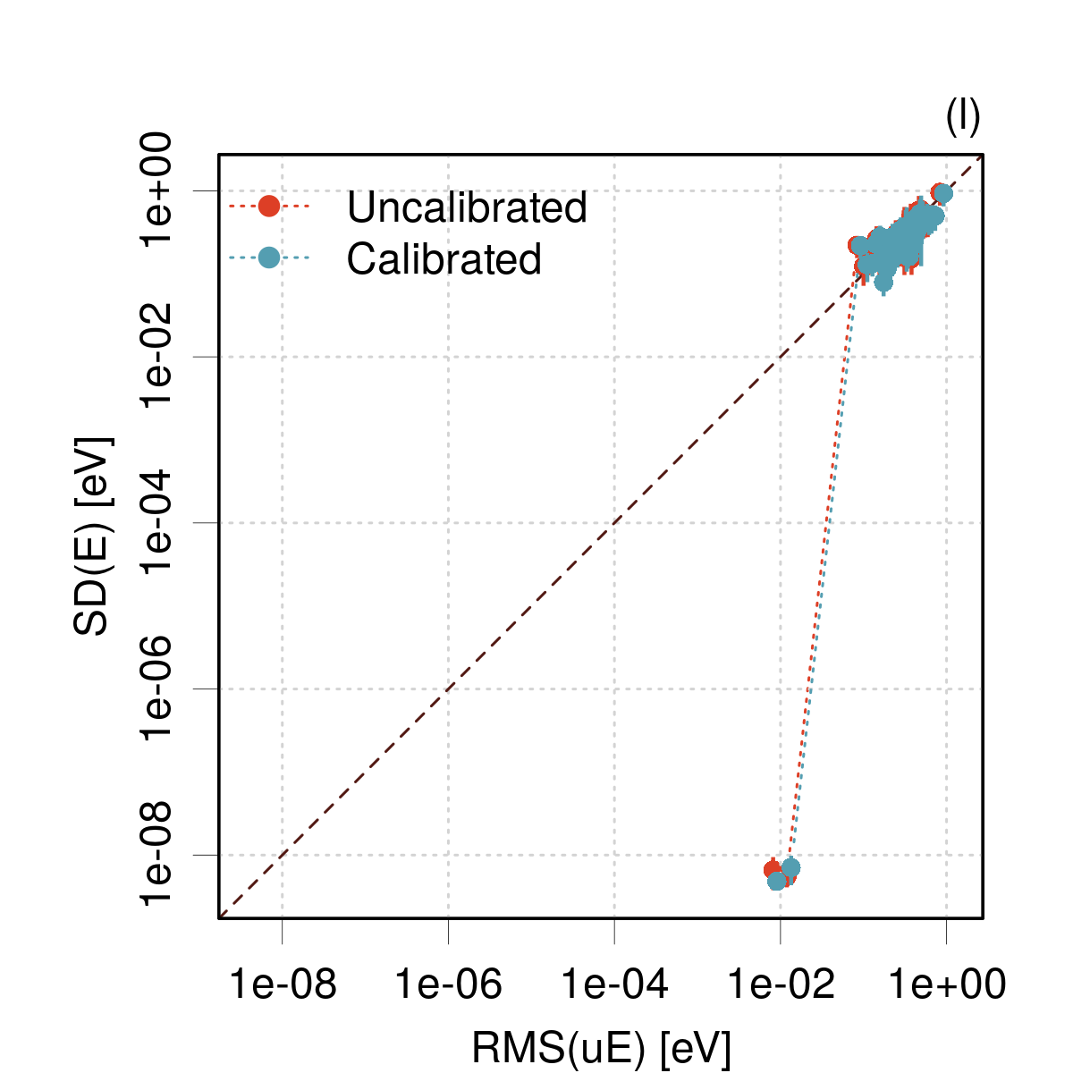
Figure A3: Case PAL2022/Perovskite_GPR_Bayesian. Impact of the number of bins on LZISD analysis and reliability diagrams: (a-f) bins with equal populations; (g-l) adaptive strategy.

The adaptive binning strategy in logarithmic uncertainty seems to be able to detect consistency problems more efficiently than binning in linear uncertainty, either with bins of same counts or same width. Of course, it does not apply to variables with negative or null values, where it can be replaced by an adaptive strategy in linear space. The adaptive binning strategy is used for the LZISD, LCP and reliability diagrams in the case studies of the present article (Sect. IV) with a starting point of $n=20$ bins.

References

- (1) G. Vishwakarma, A. Sonpal, and J. Hachmann. Metrics for Benchmarking and Uncertainty Quantification: Quality, Applicability, and Best Practices for Machine Learning in Chemistry. Trends in Chemistry, 3:146–156, 2021.
- (2) C. Gruich, V. Madhavan, Y. Wang, and B. Goldsmith. Clarifying Trust of Materials Property Predictions using Neural Networks with Distribution-Specific Uncertainty Quantification. arXiv:2302.02595, February 2023.
- (3) T. Pearce, A. Brintrup, M. Zaki, and A. Neely. High-Quality Prediction Intervals for Deep Learning: A Distribution-Free, Ensembled Approach. In International Conference on Machine Learning, pages 4075–4084. PMLR, 2018. URL: https://proceedings.mlr.press/v80/pearce18a.html.
- (4) F. Musil, M. J. Willatt, M. A. Langovoy, and M. Ceriotti. Fast and accurate uncertainty estimation in chemical machine learning. J. Chem. Theory Comput., 15:906–915, 2019.
- (5) L. Hirschfeld, K. Swanson, K. Yang, R. Barzilay, and C. W. Coley. Uncertainty Quantification Using Neural Networks for Molecular Property Prediction. J. Chem. Inf. Model., 60:3770–3780, 2020.
- (6) K. Tran, W. Neiswanger, J. Yoon, Q. Zhang, E. Xing, and Z. W. Ulissi. Methods for comparing uncertainty quantifications for material property predictions. Mach. Learn.: Sci. Technol., 1:025006, 2020.
- (7) M. Abdar, F. Pourpanah, S. Hussain, D. Rezazadegan, L. Liu, M. Ghavamzadeh, P. Fieguth, X. Cao, A. Khosravi, U. R. Acharya, V. Makarenkov, and S. Nahavandi. A review of uncertainty quantification in deep learning: Techniques, applications and challenges. Information Fusion, 76:243–297, 2021.
- (8) J. Gawlikowski, C. R. N. Tassi, M. Ali, J. Lee, M. Humt, J. Feng, A. Kruspe, R. Triebel, P. Jung, R. Roscher, M. Shahzad, W. Yang, R. Bamler, and X. X. Zhu. A Survey of Uncertainty in Deep Neural Networks. arXiv:2107.03342, 2021. arXiv: 2107.03342. URL: http://arxiv.org/abs/2107.03342.
- (9) M. Tynes, W. Gao, D. J. Burrill, E. R. Batista, D. Perez, P. Yang, and N. Lubbers. Pairwise difference regression: A machine learning meta-algorithm for improved prediction and uncertainty quantification in chemical search. J. Chem. Inf. Model., 61:3846–3857, 2021. PMID: 34347460.
- (10) E. Zelikman, C. Healy, S. Zhou, and A. Avati. CRUDE: Calibrating Regression Uncertainty Distributions Empirically. arXiv:2005.12496 [cs, stat], March 2021. arXiv: 2005.12496. URL: http://arxiv.org/abs/2005.12496.
- (11) Y. Hu, J. Musielewicz, Z. W. Ulissi, and A. J. Medford. Robust and scalable uncertainty estimation with conformal prediction for machine-learned interatomic potentials. Mach. Learn.: Sci. Technol., November 2022.
- (12) D. Varivoda, R. Dong, S. S. Omee, and J. Hu. Materials Property Prediction with Uncertainty Quantification: A Benchmark Study. arXiv:2211.02235, November 2022.
- (13) W. He and Z. Jiang. A Survey on Uncertainty Quantification Methods for Deep Neural Networks: An Uncertainty Source Perspective. arXiv:2302.13425, February 2023.
- (14) Y. Liu, M. Pagliardini, T. Chavdarova, and S. U. Stich. The Peril of Popular Deep Learning Uncertainty Estimation Methods. arXiv:2112.05000, 2021.
- (15) P. Pernot. Prediction uncertainty validation for computational chemists. J. Chem. Phys., 157:144103, 2022.
- (16) BIPM, IEC, IFCC, ILAC, ISO, IUPAC, IUPAP, and OIML. Evaluation of measurement data - Guide to the expression of uncertainty in measurement (GUM). Technical Report 100:2008, Joint Committee for Guides in Metrology, JCGM, 2008. URL: http://www.bipm.org/utils/common/documents/jcgm/JCGM_100_2008_F.pdf.
- (17) K. K. Irikura, R. D. Johnson, and R. N. Kacker. Uncertainty associated with virtual measurements from computational quantum chemistry models. Metrologia, 41:369–375, 2004.
- (18) B. Ruscic, R. E. Pinzon, M. L. Morton, G. von Laszevski, S. J. Bittner, S. G. Nijsure, K. A. Amin, M. Minkoff, and A. F. Wagner. Introduction to Active Thermochemical Tables: Several "key" enthalpies of formation revisited. J. Phys. Chem. A, 108:9979–9997, 2004.
- (19) J. P. Janet, C. Duan, T. Yang, A. Nandy, and H. J. Kulik. A quantitative uncertainty metric controls error in neural network-driven chemical discovery. Chem. Sci., 10:7913–7922, 2019.
- (20) E. Hüllermeier and W. Waegeman. Aleatoric and epistemic uncertainty in machine learning: an introduction to concepts and methods. Mach. Learn., 110:457–506, 2021.
- (21) V. Korolev, I. Nevolin, and P. Protsenko. A universal similarity based approach for predictive uncertainty quantification in materials science. Sci. Rep., 12:1–10, 2022.
- (22) A. N. Angelopoulos and S. Bates. A Gentle Introduction to Conformal Prediction and Distribution-Free Uncertainty Quantification. arXiv:2107.07511, July 2021.
- (23) V. Vovk. Conditional validity of inductive conformal predictors. In S. C. H. Hoi and W. Buntine, editors, Proceedings of the Asian Conference on Machine Learning, volume 25 of Proceedings of Machine Learning Research, pages 475–490, Singapore Management University, Singapore, 04–06 Nov 2012. PMLR.
- (24) M. Reiher. Molecule-specific uncertainty quantification in quantum chemical studies. Isr. J. Chem., 62(1-2):e202100101, 2022.
- (25) P. Pernot. Confidence curves for UQ validation: probabilistic reference vs. oracle. arXiv:2206.15272, June 2022.
- (26) T. Gneiting, F. Balabdaoui, and A. E. Raftery. Probabilistic forecasts, calibration and sharpness. J. R. Statist. Soc. B, 69:243–268, 2007.
- (27) T. Gneiting and M. Katzfuss. Probabilistic forecasting. Annu. Rev. Stat. Appl., 1:125–151, 2014.
- (28) P. Pernot. The long road to calibrated prediction uncertainty in computational chemistry. J. Chem. Phys., 156:114109, 2022.
- (29) V. Kuleshov, N. Fenner, and S. Ermon. Accurate uncertainties for deep learning using calibrated regression. In J. Dy and A. Krause, editors, Proceedings of the 35th International Conference on Machine Learning, volume 80 of Proceedings of Machine Learning Research, pages 2796–2804. PMLR, 10–15 Jul 2018. URL: https://proceedings.mlr.press/v80/kuleshov18a.html.
- (30) D. Levi, L. Gispan, N. Giladi, and E. Fetaya. Evaluating and Calibrating Uncertainty Prediction in Regression Tasks. arXiv:1905.11659, 2020. URL: http://arxiv.org/abs/1905.11659.
- (31) Y. Chung, W. Neiswanger, I. Char, and J. Schneider. Beyond pinball loss: Quantile methods for calibrated uncertainty quantification. arXiv:2011.09588, 2020.
- (32) M.-H. Laves, S. Ihler, J. F. Fast, L. A. Kahrs, and T. Ortmaier. Well-calibrated regression uncertainty in medical imaging with deep learning. In T. Arbel, I. Ben Ayed, M. de Bruijne, M. Descoteaux, H. Lombaert, and C. Pal, editors, Proceedings of the Third Conference on Medical Imaging with Deep Learning, volume 121 of Proceedings of Machine Learning Research, pages 393–412. PMLR, 06–08 Jul 2020. URL: https://proceedings.mlr.press/v121/laves20a.html.
- (33) R. Luo, A. Bhatnagar, Y. Bai, S. Zhao, H. Wang, C. Xiong, S. Savarese, S. Ermon, E. Schmerling, and M. Pavone. Local Calibration: Metrics and Recalibration. arXiv:2102.10809, February 2021.
- (34) E. Ilg, O. Çiçek, S. Galesso, A. Klein, O. Makansi, F. Hutter, and T. Brox. Uncertainty estimates and multi-hypotheses networks for optical flow. arXiv:1802.07095, 2018. URL: https://arxiv.org/abs/1802.07095.
- (35) G. Scalia, C. A. Grambow, B. Pernici, Y.-P. Li, and W. H. Green. Evaluating scalable uncertainty estimation methods for deep learning-based molecular property prediction. J. Chem. Inf. Model., 60:2697–2717, 2020.
- (36) R. N. Kacker, R. Kessel, and K.-D. Sommer. Assessing differences between results determined according to the guide to the expression of uncertainty in measurement. J. Res. Nat. Inst. Stand. Technol., 115(6):453, 2010.
- (37) M. Cauchois, S. Gupta, and J. C. Duchi. Knowing what you know: valid and validated confidence sets in multiclass and multilabel prediction. J. Mach. Learn. Res., 22:3681–3722, 2021.
- (38) S. Feldman, S. Bates, and Y. Romano. Improving Conditional Coverage via Orthogonal Quantile Regression. arXiv:2106.00394, 2021.
- (39) Note that this definition differs from the one in my previous studies, which were based on the existence of a predicted value and an expanded uncertainty, leading to zero-centered intervals that should contain the error. In the present case the intervals are error-centered, but should contain 0.
- (40) C. Guo, G. Pleiss, Y. Sun, and K. Q. Weinberger. On Calibration of Modern Neural Networks. In International Conference on Machine Learning, pages 1321–1330. 2017. URL: https://proceedings.mlr.press/v70/guo17a.html.
- (41) G. Palmer, S. Du, A. Politowicz, J. P. Emory, X. Yang, A. Gautam, G. Gupta, Z. Li, R. Jacobs, and D. Morgan. Calibration after bootstrap for accurate uncertainty quantification in regression models. npj Comput. Mater., 8:1–9, 2022.
- (42) L. I. Vazquez-Salazar, E. D. Boittier, and M. Meuwly. Uncertainty quantification for predictions of atomistic neural networks. arXiv:2207.06916, July 2022.
- (43) J. Nixon, M. Dusenberry, G. Jerfel, T. Nguyen, J. Liu, L. Zhang, and D. Tran. Measuring Calibration in Deep Learning. arXiv:1904.01685, April 2019.
- (44) K. A. Maupin, L. P. Swiler, and N. W. Porter. Validation Metrics for Deterministic and Probabilistic Data. J. Verif. Validation Uncertainty Quantif., 3:031002, 2018.
- (45) J. Busk, P. B. Jørgensen, A. Bhowmik, M. N. Schmidt, O. Winther, and T. Vegge. Calibrated uncertainty for molecular property prediction using ensembles of message passing neural networks. Mach. Learn.: Sci. Technol., 3:015012, 2022.
- (46) A. P. Soleimany, A. Amini, S. Goldman, D. Rus, S. N. Bhatia, and C. W. Coley. Evidential Deep Learning for Guided Molecular Property Prediction and Discovery. ACS Cent. Sci., 7:1356–1367, 2021.
- (47) R. F. Barber, E. J. Candès, A. Ramdas, and R. J. Tibshirani. The limits of distribution-free conditional predictive inference. arXiv:1903.04684, 2019.
- (48) R Core Team. R: A Language and Environment for Statistical Computing. R Foundation for Statistical Computing, Vienna, Austria, 2019. URL: http://www.R-project.org/.