Uncertainty quantification in neural network classifiers – a local linear approach

Abstract

Classifiers based on neural networks (nn) often lack a measure of uncertainty in the predicted class. We propose a method to estimate the probability mass function (pmf) of the different classes, as well as the covariance of the estimated pmf. First, a local linear approach is used during the training phase to recursively compute the covariance of the parameters in the nn. Secondly, in the classification phase another local linear approach is used to propagate the covariance of the learned nn parameters to the uncertainty in the output of the last layer of the nn. This allows for an efficient Monte Carlo (mc) approach for: (i) estimating the pmf; (ii) calculating the covariance of the estimated pmf; and (iii) proper risk assessment and fusion of multiple classifiers. Two classical image classification tasks, i.e., mnist, and cfar10, are used to demonstrate the efficiency the proposed method.

, , ,

1 Introduction

In this paper, the problem of quantifying the uncertainty in the predictions from a neural network (nn) is studied. The uncertainty in the prediction stems from three different sources: errors caused by the optimization algorithm that is used to train the nn, errors in the data (aleatoric uncertainty), and errors in the model (epistemic uncertainty). In this paper, the focus is on uncertainty from the two latter sources.

In numerous applications, e.g., image recognition [1], learning properties in atoms [2], and various control tasks [3, 4], nns have shown high performance. Despite their high performance, the use of nns in safety-critical applications is limited [5, 6, 7]. It is partly a consequence of the fact that their predictions usually do not come with any measure of certainty of the prediction, which is crucial to have in a decision-making process in order to know to what degree the prediction can be trusted. Moreover, the quantified measure of uncertainty can be used to detect and remove outliers in the data. Furthermore, it is not possible to fuse the prediction from the nn with information from other sensors without knowledge about the uncertainty.

Autonomous driving is an example of a safety-critical application in which it is relevant to be able to perform reliable classifications of, e.g., surrounding objects. In particular, this need was highlighted in the fatal Uber accident in 2018 where the lack of reliable classifications of surrounding objects played a role in the development of events that eventually led to the accident [8].

The problem to quantify the uncertainty in the prediction of nns has lately gained increasing attention, and numerous methods to calculate the uncertainty have been suggested [9, 10, 11, 12, 13]. For a survey of methods see [14]. The methods suggested in the literature can broadly be divided into one out of two categories. One category is based on creating an ensemble of predictions from which the uncertainty in the prediction is computed [15, 16, 17, 18, 19, 20, 21, 22]. In the other category, the nn structure is extended and the nn is trained to learn its own uncertainty [23, 24, 25, 26, 27, 28].

Concerning the first category, it has for example been suggested to create an ensemble by training multiple nns, from whose predictions the uncertainty is computed by [15]. Since training a single nn is often computationally expensive, this method has high computational complexity. In practice, it is only feasible from a computational perspective to create small ensembles. To decrease the computational complexity, it was in [16, 17] suggested to use already existing regularization techniques (dropout and batch norm) to sample values of the parameters of the nn from which these ensembles can be created. Another method to create ensembles is by sampling values of the parameters during the last part of the training phase [18, 19]. So-called test-time data augmentation methods have also been suggested to do perturbation on the test data to create an ensemble of predictions [20]. Even though the methods in [16, 17, 18, 19, 20] do not need multiple models to be trained they require multiple forward passes. Furthermore, they require specially tailored training algorithms and carefully constructed structures of the nn.

Another limitation of methods relying on creating ensembles is that they have trouble representing the uncertainty caused by the bias in the prediction from a model mismatch. The bias can be caused by an insufficiently flexible model, which could be a result of too high regularization or too low model order.

The problem can be solved by nns from the second category, i.e., where the structure of the nn is extended such that it learns its own uncertainty in the prediction. However, this requires a more intricate nn structure with tailored loss functions [23, 24, 26, 25]. As a consequence, the training becomes more complex and computationally expensive. It also makes the methods sensitive to errors caused by the training algorithm, which are not possible to learn. Furthermore, there is also a need for more data to train complex model structures.

In this paper, we address the two limitations of the aforementioned methods using classical local approximations from the area of system identification [29], which is sometimes referred to as the delta method [30, 31, 32]. For regression tasks, the delta method has previously been used to quantify the uncertainty in the prediction of nns, see e.g., [32, 33, 34, 31, 35, 36], and extended to classification tasks in [30].

2 Problem formulation and contributions

Consider the problem of learning a classifier from the training data set

$$\mathcal{T}\triangleq\{y_{n},x_{n}\}_{n=1}^{N}$$ (1)

Here $y_{n}\in\{1,\ldots,M\}$ is the class labels and $x_{n}\!\in\!\mathbb{R}^{n_{x}}$ is the input data of size $n_{x}$, e.g., pixels in an image. From a statistical point of view, the learning of the classifier can be seen as a system identification problem where a model $f(x;\theta)$ that predicts the conditional probability mass function (pmf) $p(y|x)$ of a categorical distribution, are to be identified. That is, the probability for $y=m$ given the input $x$ is modeled as

$$p(y=m|x;\theta)=f_{m}(x;\theta),\quad m=1,\ldots,M$$ (2)

Here $\theta\!\in\!\mathbb{R}^{n_{\theta}}$ denote the $n_{\theta}$-dimensional parameter vector that parameterize the model. Further, the subscript $m$ denotes the $m$:th element of the vector-valued output of the function.

To ensure that the model $f(x;\theta)$ fulfills the properties associated with pmf, i.e., $f_{m}(x;\theta)\geq 0$ $\forall m$ and $\sum_{m}f_{m}(x;\theta)=1$, it is typically structured as

$$f(x;\theta)=\text{softmax}\left(g(x;\theta)\right)$$ (3)

where

$$\text{softmax}(z)\triangleq\frac{1}{\sum_{m=1}^{M}e^{z_{m}}}\begin{bmatrix}e^{z_{1}}\\ \vdots\\ e^{z_{M}}\end{bmatrix}$$ (4)

and $g(x;\theta)$ describes the underlying model of the classifier.

In the case $g_{m}(x;\theta)=\theta^{\top}\phi_{m}(x)$, where $\phi_{m}(x)$ denotes, a possible nonlinear, transformation of the input $x$, then the model in (3) becomes a standard multinomial logistic regression model [37]. Furthermore, if the transformation $\phi_{m}(x)$ is chosen randomly, the model becomes similar to the one used in extreme learning machine classifiers [38].

If a nn is used for classification, then the model is given by

$$h^{(0)}=x,$$ (5a)

$$a^{(l+1)}=\begin{pmatrix}h^{(l)}&1\end{pmatrix}^{\top}W^{(l)},\quad l=0,\ldots,L-1,$$ (5b)

$$h^{(l)}=\sigma\big{(}a^{(l)}\big{)},\quad l=1,\ldots,L-1,$$ (5c)

$$g(x;\theta)=a^{(L)}.$$ (5d)

Here $$\sigma(\cdot) \sigma(z)=\max(0,z) a^{(l)} l h^{(l)} l W^{(L)},\ldots,W^{(0)}$$ denotes the activation function, where the ReLu function is often used. The latent variable denotes the value of all the nodes in the ’th layer of the nn, and denotes the transformation using the activation function of the values in all the nodes in the ’th layer of the nn. The parameters of the nn model consist of all the weights and biases included in the matrices , i.e.,

$$\theta =\begin{bmatrix}\text{Vec}(W^{(L)})^{\top}&\ldots&\text{Vec}(W^{(0)})^{\top}\end{bmatrix}^{\top}.$$ (5e)

Here $\text{Vec}(\cdot)$ denotes the vectorization operator.

2.1 Parameter estimation

For most nn the number of model parameters $n_{\theta}>N$ and the model parameters $\theta$ cannot be uniquely identified from the training data $\mathcal{T}$ without some regularization or prior information regarding the parameters. Let $p(\theta)$ denote the prior for the model parameters. The maximum a posteriori estimate of the model parameters is then given by

$$\hat{\theta}_{N}=\operatorname*{arg\,max}_{\theta}p(\theta|\mathcal{T})=\operatorname*{arg\,max}_{\theta}L_{N}(\theta)+\ln p(\theta),$$ (6)

where $p(\theta|\mathcal{T})$ denotes the a posteriori distribution of the parameters and

$$L_{N}(\theta)=\sum_{n=1}^{N}\ln f_{y_{n}}(x_{n};\theta)$$ (7)

denotes the cross-entropy likelihood function [37]. Here $y_{n}$ is used as an index operator for the subscript $m$ of $f_{m}(x;\theta)$.

2.2 Prediction and classification

Once the classifier has been learned, i.e., a parameter estimate $\hat{\theta}_{N}$ has been computed, then for a new input data point $x^{\star}$ the probability mass function can be predicted as

$$\hat{p}(y^{\star}=m|x^{\star};\hat{\theta}_{N})=f_{m}(x^{\star};\hat{\theta}_{N}),\quad m=1,\ldots,M$$ (8)

and the most likely class can be found as

$$\hat{y}^{\star}=\operatorname*{arg\,max}_{m}f_{m}(x^{\star};\hat{\theta}_{N}).$$ (9)

Note that, the full pmf estimate $f(x;\hat{\theta}_{N})$ is needed both for temporal fusion using several inputs from the same class and fusion over different classifiers. Furthermore, even small probabilities can pose a large risk, e.g., there might be a pedestrian in front of a car even if another harmless object is more likely according to the classifier. Hence, it is important that the prediction $\hat{p}(y^{\star}=m|x^{\star};\hat{\theta}_{N})$ is accurate. However, it is well known that due to, among other things, uncertainties in the parameter estimates $\hat{\theta}_{N}$ the disagreement between true and estimated pmf may be significant. Therefore, methods to calibrate the prediction $\hat{p}(y^{\star}|x^{\star};\hat{\theta}_{N})$ such that it better matches $p(y^{\star}|x^{\star})$ has been developed.

2.3 Temperature scaling

One of the most commonly used methods to calibrate the predicted pmf is called temperature scaling [39]. In temperature scaling $g(x;\theta)$ is scaled by a scalar quantity $T$ before the normalization by the softmax operator. With a slight abuse of notation, introduce

$$f(x^{\star};\hat{\theta}_{N},T)=\text{softmax}\left(g(x^{\star};\hat{\theta}_{N})/T\right).$$ (10)

Via the temperature scaling parameter $T$ the variations between the components (classes) in the predicted pmf can be enhanced or reduced. When $T\rightarrow 0$, then $f(x^{\star};\hat{\theta}_{N},T)\rightarrow\vec{e}_{i}$, where $\vec{e}_{i}$ denotes the $i$:th standard basis vector, thereby indicating that input $x^{\star}_{n}$ with total certainty belongs to class $i$. Similarly, when $T\rightarrow\infty$, then $f_{m}(x^{\star};\hat{\theta}_{N},T)\rightarrow 1/M$ $\forall m$, thereby indicating that input $x^{\star}_{n}$ is equally probable to belong to any of the classes.

Noteworthy is that the temperature scaling is typically done after the parameters $\theta$ have been estimated. For notational brevity, the dependency on the temperature scaling parameter $T$ will only be explicitly stated when temperature scaling is considered.

2.4 Marginalization of parameter uncertainties

A more theoretically sound approach to take the uncertainties in the parameter estimate into account is via marginalization of the pmf with respect to the parameter distribution. That is, an estimate of the pmf and its covariance are calculated as

$$f(x^{\star}|\mathcal{T})\triangleq\int_{\theta}f(x^{\star};\theta)p\big{(}\theta|\mathcal{T}\big{)}d\theta$$ (11a)

$$P^{f}\triangleq\int_{\theta}\bigl{(}f(x^{\star};\theta)-f(x^{\star}|\mathcal{T})\bigr{)}\bigl{(}\cdot\bigr{)}^{\top}p\big{(}\theta|\mathcal{T}\big{)}d\theta$$ (11b)

From hereon $(x)(\cdot)^{\top}$ is used as shorthand notation for $xx^{\top}$. The integral in (11a) is generally intractable, but can be approximated by Monte Carlo (mc) sampling as follows

$$\theta^{(k)}\sim p\big{(}\theta|\mathcal{T}\big{)},\quad k=1,2,\dots,K,$$ (12a)

$$\hat{f}(x^{\star}|\mathcal{T})=\frac{1}{K}\sum_{k=1}^{K}f(x^{\star};\theta^{(k)})$$ (12b)

$$\hat{P}^{f}=\frac{1}{K}\sum_{k=1}^{K}\bigl{(}f(x^{\star};\theta^{(k)})-\hat{f}(x^{\star}|\mathcal{T})\bigr{)}\bigl{(}\cdot\bigr{)}^{\top}.$$ (12c)

Here $K$ denotes the number of samples used in the mc sampling.

2.5 Challenges and contributions

To realize the mc scheme in (12) the posterior parameter distribution $p\big{(}\theta|\mathcal{T}\big{)}$ must be computed and samples drawn from this high-dimensional distribution. Our contributions are: (i) a local linearization approach that leads to a recursive algorithm of low complexity to compute an approximation of the posterior parameter distribution $p\big{(}\theta|\mathcal{T}\big{)}$ during the training phase; (ii) a second local linearization approach to reduce the sampling space from $n_{\theta}$ to $M$-dimensional space in the prediction phase; and as a by-product (iii) a low-complexity method for risk assessment and information fusion.

3 Posterior parameter distribution

Next, a local linearization approach that leads to a recursive algorithm of low complexity to compute an approximation of the posterior parameter distribution $p\big{(}\theta|\mathcal{T}\big{)}$ during the training phase is presented.

3.1 Laplace approximation

Assume the prior distribution for the model parameters to be normal distributed as $p(\theta)=\mathcal{N}(\theta;0,P_{0})$, i.e., $l^{2}$ regularization is used. Then a Laplace approximation of the posterior distribution $p(\theta|\mathcal{T})$ yields that [40]

$$p(\theta|\mathcal{T})\approx\mathcal{N}(\theta;\hat{\theta}_{N},P^{\theta}_{N}),$$ (13)

where

$$P^{\theta}_{N}=\left(-\frac{\partial^{2}L_{N}(\theta)}{\partial\theta^{2}}\Biggr{|}_{\theta=\hat{\theta}_{N}}+P_{0}^{-1}\right)^{-1}.$$ (14)

That is, the prior distribution is approximated by a normal distribution with a mean located at the maximum a posteriori estimate and a covariance dependent upon the shape of the likelihood function in the vicinity of the estimate. The accuracy of the approximation will depend upon the amount of information in the training data $\mathcal{T}$.

3.2 Asymptotic distribution

According to Bernstein-von Mises theorem [41], if the true model belongs to the considered model set, the maximum a posteriori estimate $\hat{\theta}$ converge in distribution to

$$\hat{\theta}_{N}\stackrel{{\scriptstyle d}}{{\longrightarrow}}\mathcal{N}(\hat{\theta}_{N};\theta_{\ast},\mathcal{I}_{\theta}^{-1}),$$ (15)

when the information in the training data $\mathcal{T}$ tends to infinity. Here, $\theta_{\ast}$ denotes the true parameters and

$$\mathcal{I}_{\theta}\triangleq-\text{E}\bigg{\{}\frac{\partial^{2}L_{N}(\theta)}{\partial\theta^{2}}\bigg{\}},$$ (16)

is the Fisher information matrix. Given the likelihood function in (7) the Fisher matrix becomes

$$\mathcal{I}_{\theta}\simeq\sum_{n=1}^{N}\sum_{m=1}^{M}\eta_{m,n}\frac{\partial g_{m}\!(x_{n};\theta)}{\partial\theta}\bigg{(}\!\frac{\partial g_{m}\!(x_{n};\theta)}{\partial\theta}\!\bigg{)}^{\!\!\top\!}$$ (17a)

where

$$\eta_{m,n}\triangleq f_{m}(x_{n};\theta)(1-f_{m}(x_{n};\theta)).$$ (17b)

See derivations in Appendix A.

3.3 Recursive computation of covariance

To compute the parameter covariance $P^{\theta}_{N}$ defined by (14), the Hessian matrix of the log-likelihood (ll) must be calculated and then inverted. This has a complexity of $\mathcal{O}(NMn_{\theta}^{2}+n_{\theta}^{3})$, which for large $n_{\theta}$ and $N$ can become intractable. However, by approximating the Hessian matrix of the ll with the Fisher information matrix as follows

$$P^{\theta}_{N}\approx\left(\mathcal{I}_{\hat{\theta}_{N}}+P_{0}^{-1}\right)^{-1},$$ (18)

the computation can be done recursively and with a complexity of $\mathcal{O}\big{(}NMn_{\theta}^{2}+NM^{3}\big{)}$. To do so, note that the $\mathcal{I}_{\theta}$ in (17) can be written in a quadratic form by defining

$$u_{m,n}\triangleq\sqrt{\eta_{m,n}}\frac{\partial g_{m}(x_{n};\theta)}{\partial\theta}\Bigl{|}_{\theta=\hat{\theta}_{N}}.$$ (19)

To compute $u_{mn}\in\mathbb{R}^{n_{\theta}}$ only the gradient of the ll in (7) is required, which is nevertheless needed for the estimation of $\theta$. Since $\mathcal{I}_{\theta}$, and so also the covariance $P^{\theta}_{N}$, can be written in a quadratic form, it is possible to update it recursively as [30]

$$K_{n} =P^{\theta}_{n}U_{n}\big{(}I_{M}\!+U^{\top}_{n}P^{\theta}_{n}U_{n}\big{)}^{-1}$$ (20a)

$$P^{\theta}_{n+1} =P^{\theta}_{n}-K_{n}U^{\top}_{n}P^{\theta}_{n},$$ (20b)

where $I_{r}$ denotes the identity matrix of size $r$. Here $P^{\theta}_{n}$ is the parameter covariance for $n$ measurements, and $U_{n}$ is defined as

$$U_{n}=\begin{bmatrix}u_{1,n}&\ldots&u_{M,n}\end{bmatrix}\in\mathbb{R}^{n_{\theta}\times M}.$$ (21)

The recursion is initialized with $P^{\theta}_{0}=P_{0}$.

3.4 Approximating the covariance

An nn often has millions of parameters which might result in the amount of data needed to store $P^{\theta}_{N}$ being larger than the available memory capacity. A common approach to handle this is to approximate $P^{\theta}_{N}$ as a block-diagonal matrix [42]. Another common approach is to use the approximation

$$P^{\theta}_{N}\approx\begin{bmatrix}P^{\theta_{r}}_{N}&0\\ 0&0\end{bmatrix},$$ (22)

where $P^{\theta_{r}}_{N}$ denotes the covariance of the estimated parameters $\theta_{r}$ corresponding to the weights and biases of the $r$ last layers in the nn [43, 30]. Depending of the number of included layers, this approximation might be more or less accurate. To compensate for the approximation error when doing the marginalization in (11), a scaling of $P^{\theta_{r}}_{N}$ with factor $T_{c}\geq 1$ can be introduced. The scaling can be estimated from validation data in a similar manner to the temperature scaling $T$ in Sec. 2.3.

4 Efficient MC sampling

With access to the parameter covariance, one can propagate the uncertainty in the parameters to uncertainty in the prediction with the delta method using the principle of marginalization. Plugging in the approximate Gaussian distribution (15) into (11a) gives

$$f(x^{\star}|\mathcal{T})=\int_{\theta}f(x^{\star};\theta)\mathcal{N}\big{(}\theta;\hat{\theta}_{N},P_{N}^{\theta}\big{)}d\theta$$ (23a)

$$P^{f}=\int_{\theta}\bigl{(}f(x^{\star};\theta)-f(x^{\star}|\mathcal{T})\bigr{)}\bigl{(}\cdot\bigr{)}^{\top}\mathcal{N}\big{(}\theta;\hat{\theta}_{N},P_{N}^{\theta}\big{)}d\theta$$ (23b)

from which mc approximation can be performed

$$\theta^{(k)}\sim\mathcal{N}\big{(}\theta;\hat{\theta}_{N},P_{N}^{\theta}\big{)},\quad k=1,2,\dots,K,$$ (24a)

$$\hat{f}(x^{\star}|\mathcal{T})=\frac{1}{K}\sum_{k=1}^{K}f\big{(}x^{\star};\theta^{(k)}\big{)}$$ (24b)

$$\hat{P}^{f}=\frac{1}{K}\sum_{k=1}^{K}\bigl{(}f(x^{\star};\theta^{(k)})-\hat{f}(x^{\star}|\mathcal{T})\bigr{)}\bigl{(}\cdot\bigr{)}^{\top}.$$ (24c)

This is a feasible solution to the problem, but it comes with a high computational cost since it requires drawing mc samples from a high-dimensional Gaussian distribution and evaluating the whole network.

4.1 Marginalization using the delta method

The delta method, see e.g., [31, 32], relies on linearization of the nonlinear model $g(x,\theta)$ and provides a remedy to the problem of sampling from the high-dimensional Gaussian distribution. The idea is to project the uncertainty in the parameters to uncertainty in the prediction before the softmax normalization (4), thereby drastically reducing the dimension of the distribution that must be sampled. Using the delta method, the uncertainty in the parameters can be propagated to the prediction before the softmax normalization as

$$p(g(x^{\star};\theta)|\mathcal{T})\approx\mathcal{N}\big{(}g(x^{\star};\theta);\hat{g}_{N},P_{N}^{g})$$ (25a)

where

$$\hat{g}_{N}=\text{E}\{g(x^{\star};\theta)\}\simeq g(x^{\star};\hat{\theta}_{N})$$ (25b)

and

$$\begin{split}P_{N}^{g}&=\mathrm{Cov}\{g(x^{\star};\theta)\}\\ &\simeq\bigg{(}\frac{\partial}{\partial\theta}g(x^{\star};\theta)\big{|}_{\theta=\hat{\theta}_{N}}\bigg{)}^{\top}\!P^{\theta}_{N}\frac{\partial}{\partial\theta}g(x^{\star};\theta)\big{|}_{\theta=\hat{\theta}_{N}}.\end{split}$$ (25c)

Using this Gaussian approximation of the parameter distribution, the mc approximation of the marginalization integral becomes

$$g^{(k)}(x^{\star})\sim\mathcal{N}\big{(}g(x^{\star},\theta);\hat{g}_{N},P_{N}^{g}),\quad k\!=\!1,2,\dots K$$ (26a)

$$f^{(k)}(x^{\star})=\mathrm{softmax}\big{(}g^{(k)}(x^{\star})\big{)},$$ (26b)

$$\hat{f}(x^{\star}|\mathcal{T})=\frac{1}{K}\sum_{k=1}^{K}f^{(k)}(x^{\star}),$$ (26c)

$$\hat{P}^{f}=\frac{1}{K}\sum_{k=1}^{K}\bigl{(}f^{(k)}(x^{\star})-\hat{f}(x^{\star}|\mathcal{T})\bigr{)}\bigl{(}\cdot\bigr{)}^{\top}.$$ (26d)

To summarize, the main idea of the delta method is linearization performed in two steps. First, the parameter uncertainty is computed using (15), and second, the uncertainty is propagated to the output of the model by (25). Hence, the delta method is a local linear approach that gives a linear approximation of a nonlinear model.

4.2 Fusion

Suppose there are a set of independent classifiers, each one providing a marginal distribution $\mathcal{N}\big{(}g_{N,c};\hat{g}_{N,c},P_{N,c}^{g})$, $c=1,\ldots,C$. Then the predictions (before the softmax normalization) from these classifiers can be fused as follows [44]

$$P_{N}^{g} =\left(\sum_{c=1}^{C}\big{(}P_{N,c}^{g}\big{)}^{-1}\right)^{-1},$$ (27a)

$$\hat{g}_{N} =P_{N}^{g}\sum_{c=1}^{C}\big{(}P_{N,c}^{g}\big{)}^{-1}\hat{g}_{N,c}.$$ (27b)

If a single classifier is used to classify a set of inputs $x^{\star}_{c}$, $c=1,\ldots,C$, known to belong to the same class $y^{\star}$, then these predictions can be fused as follows

$$P_{N}^{g} =(H^{\top}R^{-1}H)^{-1},$$ (28a)

$$\hat{g}_{N} =P_{N}^{g}H^{\top}R^{-1}z$$ (28b)

where

$$z=\begin{bmatrix}\hat{g}_{N,1}\\ \vdots\\ \hat{g}_{N,C}\end{bmatrix}\in\mathbb{R}^{CM}\quad H=\begin{bmatrix}I_{M}\\ \vdots\\ I_{M}\end{bmatrix}\in\mathbb{R}^{CM,M}$$ (28c)

and the block $$[R]_{i,j}\in\mathbb{R}^{M,M} i,j=1,\ldots,C$$, , of the covariance matrix is given by

$$[R]_{i,j}=\frac{\partial}{\partial\theta}g(x^{\star}_{i};\theta)^{\top}\big{|}_{\theta=\hat{\theta}_{N}}\!P^{\theta}_{N}\frac{\partial}{\partial\theta}g(x^{\star}_{j};\theta)\big{|}_{\theta=\hat{\theta}_{N}}.$$ (28d)

After fusion, the mc sampling in (26) can be applied as before to compute the pmf estimate.

4.3 Risk assessment

Risk assessment can be defined as the probability $r_{m}$ that $p(y^{\star}_{n}=m|x^{\star}_{n})>\gamma_{m}$. The probability $r_{m}$ can be estimated from the identified model $f_{m}(x^{\star}_{n}|\mathcal{T})$ as follows

$$\begin{split}\hat{r}_{m}&=\text{Pr}\{f_{m}(x^{\star}_{n}|\mathcal{T})>\gamma_{m}\}\\ &\simeq\frac{1}{K}\sum_{k=1}^{K}\mathbb{1}\big{(}f^{(k)}_{m}(x^{\star}_{n})>\gamma_{m}\big{)}.\end{split}$$ (29)

Here $\mathbb{1}(a>b)$ denotes the indicator function which is one if $a>b$ and zero otherwise.

5 Validation

Suppose now we have a validation data set $\mathcal{V}=\{y^{\circ}_{n},x^{\circ}_{n}\}_{n=1}^{N_{\circ}}$. How can we validate the estimated pmf $\hat{f}(x^{\circ}_{n}|\mathcal{T})$ obtained from (26)? The inherent difficulty is that the validation data, just as the training data, consists of inputs and class labels, not the actual pmf. Indeed, there is a lack of unified qualitative evaluation metrics [14]. That being said, some of the most commonly used metrics are classification accuracy, ll, Brier score, and expected calibration error (ece).

Both the negative ll and the Brier score are proper scoring rules, meaning that they emphasize careful and honest assessment of the uncertainty, and are minimized for the true probability vector [45]. However, neither of them is a measure of the calibration, i.e., reliability of the estimated pmf. Out of these metrics, only ece considers the calibration. Hence, here ece is the most important metric when evaluating a method used to measure the uncertainty [39, 46]. The calculation of the Brier score and ece, together with reliability diagrams are described next. They all can be used to tune the temperature scaling $T$ described in Section 2.3.

5.1 Brier score

The Brier score [45, 47] corresponds to the least squares fit

$$\frac{1}{N_{\circ}}\sum_{n=1}^{N_{\circ}}\sum_{m=1}^{M}\bigl{(}\delta_{m,y_{n}}-\hat{p}(y^{\circ}_{n}=m|x^{\circ}_{n})\bigr{)}^{2},$$ (30)

where $\delta_{i,j}$ denotes the Kronecker delta function. Furthermore, $\hat{p}(y^{\circ}_{n}=m|x^{\circ}_{n})$ denotes a generic pmf estimate.

5.2 Accuracy and reliability diagram

Accuracy and reliability diagrams are calculated as follows. Calculate the $J$ bin histogram defined as

$$B_{j}=\bigg{\{}n:\frac{j-1}{J}\leq\max_{m}\hat{p}(y^{\circ}_{n}=m|x^{\circ}_{n})<\frac{j}{J}\bigg{\}}$$ (31)

from the validation data. For a perfect classifier $B_{j}=\emptyset$ for $j<J$. For a classifier that is just guessing, all sets are of equal size, i.e., $|B_{j}|=|B_{i}|$ $\forall i,j$. Note that $\max_{m}\hat{p}(y^{\circ}_{n}=m|x^{\circ}_{n})\geq 1/M$, so the first bins will be empty if $J>M$.

The accuracy of the classifier is calculated by comparing the size of each set with the actual classification performance within the set. That is,

$$\text{acc}(B_{j})=\frac{1}{|B_{j}|}\sum_{n\in B_{j}}\mathbb{1}\big{(}\hat{y}^{\circ}_{n}=y^{\circ}_{n}\big{)}$$ (32a)

where

$$\hat{y}^{\circ}_{n}=\operatorname*{arg\,max}_{m}\hat{p}(y^{\circ}_{n}=m|x^{\circ}_{n})$$ (32b)

A reliability diagram is a plot of the accuracy versus the confidence, i.e., the predicted probability frequency. A classifier is said to be calibrated if the slope of the bins is close to one, i.e., when $\text{acc}(B_{j})=(j-0.5)/J$.

5.3 Confidence and expected calibration error

Instead of certainty, from hereon the standard, and equivalent, notion of confidence will be used [39, 46]. The mean confidence in a set is denoted $\text{conf}(B_{j})$ and is defined as

$$\text{conf}(B_{j})=\frac{1}{|B_{j}|}\sum_{n\in B_{j}}\max_{m}\hat{p}(y^{\circ}_{n}=m|x^{\circ}_{n}),$$ (33)

This is a measure of how much the classifier trusts its estimated class labels. In contrast to the accuracy it does not depend on the annotated class labels $y_{n}$. Comparing accuracy to confidence gives the ece, defined as

$$\text{{ece}}=\sum_{j}^{J}\frac{1}{|B_{j}|}|\text{acc}(B_{j})-\text{conf}(B_{j})|.$$ (34)

A small value indicates that the weight is a good measure of the actual performance.

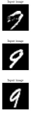
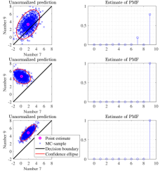
Figure 1: Example of classification using (26). Left: inputs $x^{\circ}_{n}$. Middle: Ellipse representation of $P^{g}_{N}$, mc samples $g^{(k)}(x^{\circ}_{n})$ and decision line between the classes representing 7 and 9. Right: Estimated pmf $\hat{f}(x^{\circ}|\mathcal{T})$.

6 Experiment study

To illustrate the application of the proposed method to quantify uncertainty in the prediction, two datasets were used. First, an nn was trained using the mnist dataset [48] to classify images of handwritten digits. Second, an nn was trained on the cfar10 dataset [49] to classify images of ten different objects including e.g., cars, cats, and aircraft.

6.1 Classification setup

For the two datasets, the structure of the nn was chosen differently. For the mnist dataset, a five-layer nn with fully-connected nodes were used. For the cfar10 dataset, a LeNet5-inspired structure was used with six convolutional layers followed by four fully connected layers. However, for both datasets the three last layers were chosen to have the same structure, i.e., they were fully connected with $n_{W,L-2}=100$, $n_{W,L-1}=40$, and $n_{W,L}=10$. To decrease the size of the parameter covariance used by the delta method, as described in Sec. 3.4 the first part of the nn was assumed fixed and used to create high-level features. Since the structure of the later layers was chosen identically, the parametric models trained on the two datasets had $n_{\bm{\theta}}=4450$ parameters.

To estimate the model parameters $\theta$ of the nn, the adam optimizer [50] was used. The standard adam optimizer settings, together with an initial learning rate of $10^{-4}$ and $l^{2}$ regularization of $10^{-4}$, were used. Three and ten epochs were used with the mnist dataset and cfar10 dataset, respectively.

6.2 Illustration of the uncertainties in the predictions

The low-dimensional space of the output from $g(x^{\circ}_{n};\hat{\theta}_{N})$ is particularly interesting to study when trying to understand how the uncertainty in the parameter estimate $\hat{\theta}_{N}$ affects the classification. Even if the parameter covariance $P^{\theta}_{N}$ is constant and only depends on the training data, the covariance $P^{g}_{N}$ depends on the input $x_{n}$. Fig. 1 illustrates this via an example where we concentrate our study on the decision between just a subset of the number of classes in the mnist dataset, even though the final decision is over all classes. More generally, for some inputs $x^{\circ}_{n}$ that are located in a dense region in the space of the training data, the covariance $P^{g}_{N}$ is small, but for an input $x^{\circ}_{n}$ that is very far from the training data in some norm, the covariance $P^{g}_{N}$ can be quite large. This indicates that the parameter estimate is quite sensitive in some directions. That means that the output can also be quite sensitive, and a small change in the parameters can give a completely different output. This can be seen in the two examples on the bottom part of Fig. 1. Even though the estimate of the pmf looks similar (especially for the two classes under consideration), by studying the unnormalized prediction $g(x^{\circ}_{n};\hat{\theta}_{N})$ it is clear that the prediction in the middle has a higher uncertainty compared to the bottom one.

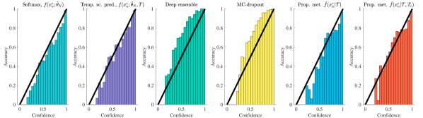
Figure 2: Reliability diagrams for prediction on the mnist dataset. The diagrams illustrate the six different methods to measure the confidence in the prediction described in Sec. 6.3. A calibration line is also shown in black.

Table 1: Computed performance measure for the two datasets. The arrows indicate whether a high or low value is preferable.

	mnist				cfar10
Method	acc. $\uparrow$	ll $(10^{3})$ $\uparrow$	Brier score $\downarrow$	ece $\downarrow$	acc. $\uparrow$	ll $(10^{3})$ $\uparrow$	Brier score $\downarrow$	ece $\downarrow$
Standard $f(x^{\circ}_{n};\hat{\theta}_{N})$	91$\%$	7.886	0.134	1.078	83$\%$	7.904	0.291	1.328
Temp. sc. $f(x^{\circ}_{n};\hat{\theta}_{N},T)$	91$\%$	7.818	0.133	0.951	83$\%$	7.740	0.269	0.612
Deep ensemble	96$\%$	7.856	0.080	2.868	87$\%$	7.834	0.191	1.479
mc-dropout	93$\%$	7.424	0.123	2.424	81$\%$	9.935	0.301	2.829
Prop. met. $\hat{f}(x^{\circ}_{n}|\mathcal{T})$	91$\%$	7.845	0.151	1.242	83$\%$	8.176	0.243	2.140
Prop. met. $\hat{f}(x^{\circ}_{n}|\mathcal{T},T_{c})$	91$\%$	7.763	0.151	0.821	82$\%$	7.545	0.239	0.540

6.3 Results on quantifying the uncertainty

Six different methods to quantify the uncertainty in the classification, i.e., to estimate $p(y^{\circ}_{n}=m|x^{\circ}_{n})$, were evaluated. These are:

1. Standard method, i.e., $\hat{p}(y^{\circ}_{n}=m|x^{\circ}_{n})=f_{m}(x^{\circ}_{n};\hat{\theta}_{N})$.

2. Temp. scaling, i.e., $\hat{p}(y^{\circ}_{n}=m|x^{\circ}_{n})=f_{m}(x^{\circ}_{n};\hat{\theta}_{N},T)$.

3. Deep ensemble, i.e., $\hat{p}(y^{\circ}_{n}=m|x^{\circ}_{n})$ is estimated using the ensemble method in [15]; number of trained nns are 50 for mnist and 10 for cfar10.

4. mc-dropout, i.e., $\hat{p}(y^{\circ}_{n}=m|x^{\circ}_{n})$ is estimated using the ensemble method in [16]; $50$ samples of the parameters are used to create the ensemble.

5. Proposed method, i.e., $\hat{p}(y^{\circ}_{n}=m|x^{\circ}_{n})=\hat{f}_{m}(x^{\circ}_{n}|\mathcal{T})$.

6. Proposed method with scaled covariance, i.e., $\hat{p}(y^{\circ}_{n}=m|x^{\circ}_{n})=\hat{f}_{m}(x^{\circ}_{n}|\mathcal{T},T_{c})$, but with the covariance $P_{N}^{g}$ in (25) scaled with a factor $T_{c}$.

In Fig. 2, the reliability diagram for the six different methods to quantify the uncertainty in the prediction of the nn described in Sec. 6.3 is shown. Neither computing the uncertainty in the prediction using the softmax (i), deep ensembles (iii), mc-dropout (iv), or the proposed method without scaled covariance (v) gives calibrated estimates of the uncertainty. To get well-calibrated estimates of the uncertainty either the proposed method with scaled covariance (vi) or temperature scaling (ii) should be used. Finding $T$ and $T_{c}$ is commonly done by minimizing the ece. However, increasing the scaling factor decreases the ll. Hence, there is a trade-off between high ll and low ece. In Table 1, the accuracy, ll, Brier score, and ece are shown for six different methods to quantify the uncertainty in the prediction of the nn. The methods are evaluated both using the mnist and cfar10 datasets. Table 1 shows that the proposed method attains the lowest ece for both datasets. This while still having reasonably good performance in terms of accuracy, ll, and Brier score.

7 Summary and Conclusion

A method to estimate the uncertainty in classification performed by a neural network has been proposed. The method also enables information fusion in applications where multiple independent neural networks are used for classification, or when a single neural network is used to classify a sequence of inputs known to belong to the same class. The method can also be used for statistical risk assessment.

The proposed method is based on a local linear approach and consists of two steps. In the first step, an approximation of the posterior distribution of the estimated neural network parameters is calculated. This is done using a Laplacian approximation where the covariance of the parameters is calculated recursively using the structure of the Fisher information matrix. In the second step, an estimate of the PMF is calculated where the effect of the uncertainty in the estimated parameters is considered using marginalization over the posterior distribution of the parameter estimate. This is done by propagating the uncertainty in the estimated parameters to the uncertainty in the output of the last layer in the neural network using a second local linear approach. The uncertainty in the output of the last layer is approximated as a Gaussian distribution of the same dimension as the number of classes. The PMF and its covariance are then calculated via MC sampling, where samples are drawn from this low-dimensional distribution.

The proposed method has been evaluated on two classical classification datasets; MNIST and CFAR10. Neural networks with standard architectures were used. To handle a large number of parameters in these network architectures, only the parameters of the last layer were considered in the uncertainty computations. The results, in terms of ECE, show that the proposed method in its standard form yielded a similar performance as standard methods which do not take the uncertainty in the estimated parameters into account. However, when using a rescaled parameter covariance matrix, used to compensate for the fact that only the uncertainty from the parameters in the last layers was considered, a significant reduction in the ECE was observed. This indicates that the proposed method works, but that more advanced low-rank methods to approximate the parameter covariance are needed. This is a direction for future research.

This work is supported by Sweden’s innovation agency, Vinnova, through project iQDeep (project number 2018-02700).

Appendix A Derivation of Fisher Information Matrix

To calculate the Fisher information matrix in (17), it is necessary to compute the Hessian of the ll with respect to $\theta$. To do so, note that

$$\frac{\partial f_{j}(x_{n},\theta)}{\partial g_{i}(x_{n};\theta)}=f_{j}(x_{n},\theta)(\delta_{i,j}-f_{i}(x_{n},\theta))$$ (35)

Hence, it holds that

$$\frac{\partial\ln f_{y_{n}}(x_{n};\theta)}{\partial g(x_{n};\theta)}=\vec{e}_{y_{n}}-f(x_{n};\theta).$$ (36)

Using the chain rule the first derivative of the ll (7) can be computed as

$$\frac{\partial L_{N}(\theta)}{\partial\theta}=\sum_{n=1}^{N}\frac{\partial g(x_{n};\theta)^{\top}}{\partial\theta}(\vec{e}_{y_{n}}-f(x_{n};\theta))$$ (37a)

$$=\sum_{n=1}^{N}\sum_{m=1}^{M}\bigl{(}\delta_{m,y_{n}}-f_{m}(x_{n},\theta)\bigr{)}\frac{\partial g_{m}(x_{n};\theta)}{\partial\theta}.$$ (37b)

Differentiation of (37) with respect to $\theta$ gives

$$\frac{\partial^{2}L_{N}(\theta)}{\partial\theta^{2}}=\sum_{n=1}^{N}\sum_{m=1}^{M}\bigl{(}\delta_{m,y_{n}}-f_{m}(x_{n},\theta)\bigr{)}\frac{\partial^{2}g_{m}(x_{n};\theta)}{\partial\theta^{2}}$$

$$-\eta_{m,n}\frac{\partial g_{m}(x_{n};\theta)}{\partial\theta}\bigg{(}\frac{\partial g_{m}(x_{n};\theta)}{\partial\theta}\bigg{)}^{\!\top\!}.$$ (38a)

with $\eta_{m,n}$ defined in (17b). And the Fisher information matrix then becomes

$$\mathcal{I}_{\theta}=-\text{E}\bigg{\{}\frac{\partial^{2}\ln L_{N}(\theta)}{\partial\theta^{2}}\bigg{\}}$$ (39a)

$$=-\sum_{n=1}^{N}\sum_{m=1}^{M}\bigl{(}\text{E}\{\delta_{m,y_{n}}\}-f_{m}(x_{n},\theta)\bigr{)}\frac{\partial^{2}g_{m}(x_{n};\theta)}{\partial\theta^{2}}$$

$$+\eta_{m,n}\frac{\partial g_{m}(x_{n};\theta)}{\partial\theta}\bigg{(}\frac{\partial g_{m}(x_{n};\theta)}{\partial\theta}\bigg{)}^{\!\top\!}$$ (39b)

$$\simeq\eta_{m,n}\frac{\partial g_{m}(x_{n};\theta)}{\partial\theta}\bigg{(}\frac{\partial g_{m}(x_{n};\theta)}{\partial\theta}\bigg{)}^{\!\top\!}.$$ (39c)

The last approximative equality follows from that $\text{E}\{\delta_{m,y_{n}}\}=p(y_{n}=m|x_{n})$ and that $f_{m}(x_{n},\theta)$ is an unbiased estimate of $p(y_{n}=m|x_{n})$ when the information in the training data tends to infinity.

References

- Krizhevsky et al. [2012] Krizhevsky, A.; Sutskever, I.; Hinton, G. E. Imagenet classification with deep convolutional neural networks. Adv. in Neural Inf. Process. Syst. (NIPS) 25. Lake Tahoe, NV USA, 2012; pp 1097–1105, 3-8 Dec.
- Gilmer et al. [2017] Gilmer, J. et al. Neural message passing for quantum chemistry. Proc. of the 34th Int. Conf. on Mach. Learn. (ICML). Sydney, Australia, 2017; pp 1263–1272, 06–11 Aug.
- Li et al. [2017] Li, Q. et al. Deep neural networks for improved, impromptu trajectory tracking of quadrotors. Proc. of IEEE Int. Conf. on Robot. and Autom. (ICRA). Singapore, Singapore, 2017; pp 5183–5189, 19 May–3 June.
- Karlsson and Hendeby [2021] Karlsson, R.; Hendeby, G. Speed Estimation From Vibrations Using a Deep Learning CNN Approach. IEEE Sensors Letters. 2021; pp 1–4.
- Grigorescu et al. [2020] Grigorescu, S.; Trasnea, B.; Cocias, T.; Macesanu, G. A survey of deep learning techniques for autonomous driving. J. of Field Robotics. 2020; pp 362–386.
- Bagloee et al. [2016] Bagloee, S. A.; Tavana, M.; Asadi, M.; Oliver, T. Autonomous vehicles: challenges, opportunities, and future implications for transportation policies. J. of Modern Trans. 2016; pp 284–303.
- Paleyes et al. [2020] Paleyes, A.; Urma, R.-G.; Lawrence, N. D. Challenges in deploying machine learning: a survey of case studies. Adv. in Neural Inf. Process. Syst. (NIPS) 34 Workshop: ML Retrospectives, Surveys & Meta-Analyses (ML-RSA). Virtual, 2020.
- NTSB [2018] NTSB, Highway Accident Report HAR-19/03 HWY18MH010; Technical Specification (TS), 2018.
- D’Amour et al. [2020] D’Amour, A. et al. Underspecification presents challenges for credibility in modern machine learning. arXiv preprint arXiv:2011.03395. 2020.
- Ghahramani [2015] Ghahramani, Z. Probabilistic machine learning and artificial intelligence. Nature. 2015; pp 452 – 459.
- Patel and Waslander [2022] Patel, K.; Waslander, S. Accurate Prediction and Uncertainty Estimation using Decoupled Prediction Interval Networks. arXiv preprint arXiv:2202.09664. 2022.
- Ovadia et al. [2019] Ovadia, Y. et al. Can you trust your model’s uncertainty? Evaluating predictive uncertainty under dataset shift. Adv. in Neural Inf. Process. Syst. (NIPS) 33. Vancouver, Canada, 2019; 8–14 Dec.
- Lin et al. [2022] Lin, S.; Clark, R.; Trigoni, N.; Roberts, S. Uncertainty Estimation with a VAE-Classifier Hybrid Model. Proc. of IEEE Int. Conf. on Acoust., Speech and Signal Processing (ICASSP). Singapore, Singapore,, 2022; pp 3548–3552, 22–17 May.
- Gawlikowski et al. [2021] Gawlikowski, J. et al. A survey of uncertainty in deep neural networks. arXiv preprint arXiv:2107.03342. 2021.
- Lakshminarayanan et al. [2017] Lakshminarayanan, B.; Pritzel, A.; Blundell, C. Simple and scalable predictive uncertainty estimation using deep ensembles. Adv. in Neural Inf. Process. Syst. (NIPS) 31. 2017; Long Beach, CA, USA, 4–9 Dec.
- Gal and Ghahramani [2016] Gal, Y.; Ghahramani, Z. Dropout as a Bayesian Approximation: Representing Model Uncertainty in Deep Learning. Proc. of the 33td Int. Conf. on Mach. Learn. (ICML). New York, NY, USA, 2016; pp 1050–1059, 20–22 Jun.
- Teye et al. [2018] Teye, M.; Azizpour, H.; Smith, K. Bayesian Uncertainty Estimation for Batch Normalized Deep Networks. Proc. of the 35th Int. Conf. on Mach. Learn. (ICML). 2018; pp 4907–4916, Stockholm, Sweden, 6–11 Jul.
- Maddox et al. [2019] Maddox, W. J. et al. A simple baseline for bayesian uncertainty in deep learning. Adv. in Neural Inf. Process. Syst. (NIPS) 33. Vancouver, Canada, 2019; 8–14 Dec.
- Osawa et al. [2019] Osawa, K. et al. Practical deep learning with Bayesian principles. Adv. in Neural Inf. Process. Syst. (NIPS) 33. Vancouver, Canada, 2019; 8–14 Dec.
- Ayhan and Berens [2018] Ayhan, M. S.; Berens, P. Test-time data augmentation for estimation of heteroscedastic aleatoric uncertainty in deep neural networks. 1st Conf. on Medical Imaging with Deep Learn. (MIDL). Amsterdam, The Netherlands, 2018; 4–6 Jul.
- Ilg et al. [2018] Ilg, E. et al. Uncertainty estimates and multi-hypotheses networks for optical flow. Proc. of 15th European Conf. on Comput. Vision (ECCV). Munich, Germany, 2018; pp 652–667, 8-14 Sep.
- Carannante et al. [2021] Carannante, G.; Bouaynaya, N. C.; Mihaylova, L. An Enhanced Particle Filter for Uncertainty Quantification in Neural Networks. Proc. of IEEE 24th Int. Conf. on Inf. Fusion (FUSION). Sun City, South Africa/ Virtual, 2021; pp 1–7, Nov 1-4.
- Charpentier et al. [2020] Charpentier, B.; Zügner, D.; Günnemann, S. Posterior network: Uncertainty estimation without ood samples via density-based pseudo-counts. Virtual, 2020.
- Kendall and Gal [2017] Kendall, A.; Gal, Y. What Uncertainties Do We Need in Bayesian Deep Learning for Computer Vision? Adv. in Neural Inf. Process. Syst. (NIPS) 31. 2017; pp 5574–5584, Long Beach, CA, USA, 4–9 Dec.
- Gustafsson et al. [2020] Gustafsson, F. K.; Danelljan, M.; Bhat, G.; Schön, T. B. Energy-Based Models for Deep Probabilistic Regression. Proc. of 16th European Conf. on Comput. Vision (ECCV). Glasgow, UK/Online, 2020; pp 325–343, 23-28 Aug.
- Blundell et al. [2015] Blundell, C.; Cornebise, J.; Kavukcuoglu, K.; Wierstra, D. Weight Uncertainty in Neural Networks. Proc. of the 32nd Int. Conf. on Mach. Learn. (ICML). Lille, France, 2015; pp 1613–1622, 6–11 Jul.
- Izmailov et al. [2021] Izmailov, P.; Nicholson, P.; Lotfi, S.; Wilson, A. G. Dangers of Bayesian model averaging under covariate shift. Adv. in Neural Inf. Process. Syst. (NIPS) 35. 2021; New Orleans, LA, USA.
- Eldesokey et al. [2020] Eldesokey, A.; Felsberg, M.; Holmquist, K.; Persson, M. Uncertainty-aware cnns for depth completion: Uncertainty from beginning to end. Proceedings of the IEEE/CVF Conference on Computer Vision and Pattern Recognition. 2020; pp 12014–12023.
- Ljung [1999] Ljung, L. System identification: theory for the user (2nd edition); PTR Prentice Hall: Upper Saddle River, NJ, USA, 1999.
- Malmström et al. [2022] Malmström, M.; Skog, I.; Axehill, D.; Gustafsson, F. Detection of outliers in classification by using quantified uncertainty in neural networks. Proc. of IEEE 25th Int. Conf. on Inf. Fusion (FUSION). Linköping, Sweden, 2022; Jul 4-7.
- Malmström [2021] Malmström, M. Uncertainties in Neural Networks A System Identification Approach. Licentiate Thesis, Dept. Elect. Eng., Linköping University, Linköping, Sweden, 2021.
- Liero and Zwanzig [2011] Liero, H.; Zwanzig, S. Introduction to the theory of statistical inference; Chapman and Hall CRC Texts in Statistical Science, Boca Raton, FL, USA, 2011.
- Hwang and Ding [1997] Hwang, J. T. G.; Ding, A. A. Prediction Intervals for Artificial Neural Networks. J. Am. Stat. Assoc. (JSTOR). 1997; pp 748–757.
- Rivals and Personnaz [2000] Rivals, I.; Personnaz, L. Construction of confidence intervals for neural networks based on least squares estimation. Elsevier J. Neural Netw. 2000; pp 463–484.
- Immer et al. [2021] Immer, A.; Korzepa, M.; Bauer, M. Improving predictions of Bayesian neural nets via local linearization. Proc. of 24nd Int. Conf. on Artificial Intell. and Statistics. (AISTATS). San Diego, CA, USA, 2021; pp 703–711, 13-15 Apr.
- Deng et al. [2022] Deng, Z.; Zhou, F.; Zhu, J. Accelerated Linearized Laplace Approximation for Bayesian Deep Learning. arXiv preprint arXiv:2210.12642 2022,
- Lindholm et al. [2022] Lindholm, A.; Wahlström, N.; Lindsten, F.; Schön, T. B. Machine Learning: A First Course for Engineers and Scientists; Cambridge University Press, 2022.
- Huang et al. [2006] Huang, G.-B.; Zhu, Q.-Y.; Siew, C.-K. Extreme learning machine: theory and applications. Neurocomputing. 2006; pp 489–501.
- Guo et al. [2017] Guo, C.; Pleiss, G.; Sun, Y.; Weinberger, K. Q. On calibration of modern neural networks. Proc. of the 34th Int. Conf. on Mach. Learn. (ICML). Sydney, Australia, 2017; pp 1321–1330, 06–11 Aug.
- Bishop [2006] Bishop, C. M. Pattern Recognition and Machine Learning; Springer, 2006; New York, NY, USA.
- Johnstone [2010] Johnstone, I. High dimensional Bernstein-von Mises: simple examples. Institute of Mathematical Statistics collections 2010, 6, 87–98.
- Martens and Grosse [2015] Martens, J.; Grosse, R. Optimizing neural networks with kronecker-factored approximate curvature. Proc. of the 32nd Int. Conf. on Mach. Learn. (ICML). Lille, France, 2015; 6–11 Jul.
- Kristiadi et al. [2020] Kristiadi, A.; Hein, M.; Hennig, P. Being bayesian, even just a bit, fixes overconfidence in relu networks. Proc. of the 37th Int. Conf. on Mach. Learn. (ICML). Online, 2020; 13-18 July.
- Gustafsson [2018] Gustafsson, F. Statistical Sensor Fusion; Studentlitteratur: Lund Sweden, 2018.
- Gneiting and Raftery [2007] Gneiting, T.; Raftery, A. E. Strictly proper scoring rules, prediction, and estimation. J. of the American Statistic. Association. 2007; pp 359–378.
- Vaicenavicius et al. [2019] Vaicenavicius, J. et al. Evaluating model calibration in classification. Proc. of 22nd Int. Conf. on Artificial Intell. and Statistics. (AISTATS). Naha, Okinawa, Japan, 2019; pp 3459–3467, 16-18 Apr.
- Wójcik et al. [2022] Wójcik, B. et al. SLOVA: Uncertainty estimation using single label one-vs-all classifier. Applied Soft Computing. 2022; p 109219.
- LeCun et al. [1998] LeCun, Y.; Cortes, C.; Burges, C. J. The MNIST database of handwritten digits. 1998; http://yann.lecun.com/exdb/mnist/.
- Krizhevsky [2009] Krizhevsky, A. Learning multiple layers of features from tiny images. M.Sc. thesis, University of Toronto, Canada, 2009.
- Kingma and Ba [2015] Kingma, D. P.; Ba, J. Adam: A Method for Stochastic Optimization. Proc. of 3rd Int. Conf. for Learn. Representations (ICLR). 2015; San Diego, CA, USA.