FedACK: Federated Adversarial Contrastive Knowledge Distillation for Cross-Lingual and Cross-Model Social Bot Detection

Abstract.

Social bot detection is of paramount importance to the resilience and security of online social platforms. The state-of-the-art detection models are siloed and have largely overlooked a variety of data characteristics from multiple cross-lingual platforms. Meanwhile, the heterogeneity of data distribution and model architecture make it intricate to devise an efficient cross-platform and cross-model detection framework. In this paper, we propose FedACK, a new federated adversarial contrastive knowledge distillation framework for social bot detection. We devise a GAN-based federated knowledge distillation mechanism for efficiently transferring knowledge of data distribution among clients. In particular, a global generator is used to extract the knowledge of global data distribution and distill it into each client’s local model. We leverage local discriminator to enable customized model design and use local generator for data enhancement with hard-to-decide samples. Local training is conducted as multi-stage adversarial and contrastive learning to enable consistent feature spaces among clients and to constrain the optimization direction of local models, reducing the divergences between local and global models. Experiments demonstrate that FedACK outperforms the state-of-the-art approaches in terms of accuracy, communication efficiency, and feature space consistency.

1. Introduction

Social bots imitate human behaviors on social networks such as Twitter, Facebook, Instagram, etc. (Yardi et al., 2010). Millions of bots, typically controlled by automated programs or platform APIs (Abokhodair et al., 2015), attempt to sneak into genuine users as a disguise to pursue malicious goals such as actively engaging in election interference (Deb et al., 2019; Ferrara et al., 2020), misinformation dissemination (Cresci, 2020), and privacy attacks (Varol et al., 2017). Bots are also involved in spreading extreme ideologies (Berger and Morgan, 2015; Ferrara et al., 2016), posing threats to online communities. Effective bot detection is necessitated by the jeopardized user experience on social media platforms and the induction of unfavorable social effects.

There is a new yet understudied problem in bot detection – a society of bots tend to be exposed to multiple social platforms and behave as collaborative cohorts. Existing bot detection solutions largely rely on user property features extracted from metadata (D’Andrea et al., 2015; Yang et al., 2020), or features derived from textual data such as a tweet post (Wei and Nguyen, 2019; Feng et al., 2021a), before adopting graph-based techniques to explore neighborhood information (Zhao et al., 2020; Feng et al., 2022; Yang et al., 2022). While such models can uncover camouflage behaviors, they are siloed and subject to the amount, shape, and quality of platform-specific data. To this end, Federated Learning (FL) has becomes the main driving force of model training across heterogeneous platforms without disclosing local private datasets. Some studies (Zhu et al., 2021; Rasouli et al., 2020; Zhang et al., 2022; Zhang, 2022) augmented FL by Generative Adversarial Networks (GANs) and Knowledge Distillation (KD) in a data-free manner to safeguard privacy against intrusions. However, they have the following limitations:

i) Restriction to homogeneous model architecture. As FL models assume homogeneous model architecture on a per client basis – which however no longer holds – participants are stringently required to conform to the same model architecture managed by a central server. It is therefore imperative to enable each individual platform to customize heterogeneous models as per unique data characteristics. ii) Inconsistent feature learning spaces. The state-of-the-art Federated KD approaches are largely based on image samples and assume consistent feature space. However, the distinction between global and local data distribution tends to result in non-negligible model drift and inconsistent feature learning spaces, which will in turn cause performance loss. It is highly desirable to align feature spaces among different clients to improve the global model performance. iii) Sensitivity to content language. Textual data based anomaly detection approaches to date are sensitive to the languages that the model is built upon. Existing solutions for cross-lingual content detection in online social networks either substantially raise computational costs (Du et al., 2021; Zia et al., 2022; De et al., 2022) or require labor-intensive feature engineering to identify cross-lingual invariant features (Steimel et al., 2019; Dementieva and Panchenko, 2021; Chu et al., 2021). Arguably, how to incorporate into a synergetic model a variety of customized models with heterogeneous data in different languages to enable consistent feature learning space is still under-explored.

This paper proposes FedACK, a novel bot detection framework through Federated Adversarial learning Contrastive learning and Knowledge distillation. FedACK envisions to enable personalization of local models in a consistent feature space across different languages (see Fig. 1). We present a new federated GAN-based knowledge distillation architecture – a global generator is used to extract the knowledge of global data distribution and to distill the knowledge into each client’s local model. We elaborate two discriminators – both globally shared and local – to enable customized model design and use a local generator for data enhancement with hard-to-decide samples. Specifically, the local training on each client side is regarded as a multi-stage adversarial learning procedure to efficiently transfer data distribution knowledge to each client and to learn consistent feature spaces and decision boundaries. We further exploit contrastive learning to constrain the optimization direction of local models and reduce the divergences between local and global models. To replicate non-IID data distribution across multi-platforms, we employ two real-world Twitter datasets, partitioned by the Dirichlet distribution. Experiment shows that FedACK outperforms the state-of-the-art approaches on accuracy and achieves competitive communication efficiency and consistent feature space. This work makes the following contributions.

• To the best of our knowledge, FedACK is the first social bot detection solution based on federated knowledge distillation that envisions cross-lingual and cross-model bot detection.

• contrast and adversarial learning mechanisms for enabling consistent feature space for better knowledge transfer and representation when tackling non-IID data and data scarcity among clients.

• FedACK outperforms other FL-based approaches by up to 15.19% accuracy improvement in high heterogeneity scenarios, and achieves up to 4.5x convergence acceleration against the 2nd fastest method.

To enable replication and foster research, FedACK is publicly available at: https://github.com/846468230/FedACK.

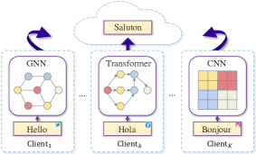
Figure 1. Incorporating multiple social platforms with heterogeneous languages, context spaces and model architectures

2. Preliminaries

2.1. Background

Federated learning (FL). FL is a distributed learning paradigm that allows clients to perform local training before aggregation without sharing clients’ private data (Konečný et al., 2016; McMahan et al., 2017; Bonawitz et al., 2017; Peng et al., 2021; Liu et al., 2022). While promising, FL can have inferior performance particularly when training data is not independent and identically distributed (Non-IID) on local devices (Zhao et al., 2018; Li et al., 2020), which could make the model deflected to a local optimum (Karimireddy et al., 2020). Most of the existing works mainly fall into two categories. The first is introducing additional data or using data enhancement to address model drift issue caused by the non-IID data. FedGAN (Rasouli et al., 2020) trains a GAN to tackle the non-IID data challenge in a communication efficient way but inevitably produces bias. FedGen (Zhu et al., 2021) and FedDTG (Zhang, 2022) utilize generator to simulate the global data distribution to improve performance. The second category mainly focuses on local regularization. FedProx (Li et al., 2020) adds an optimization item to local training, and SCAFFOLD (Karimireddy et al., 2020) uses control variants to correct the client-drift in local updates while guaranteeing a faster convergence rate. FedDyn (Acar et al., 2021) and MOON (Li et al., 2021b) constrain the direction of local model updates by comparing the similarity between model representations to align the local and global optimization objectives. However, these approaches either direct model aggregation to get the global model that causes non-negligible performance deterioration (Singh and Jaggi, 2020) or neglect the impact of data heterogeneity, which may lead to knowledge loss of local data distribution during the model aggregation.

Federated knowledge distillation (KD). KD is first introduced to use compact models to approximate the function learned by larger models (Buciluǎ et al., 2006). Knowledge is formally referred to as the softened logits, and in a typical KD, a student model absorbs and mimics the knowledge from teacher models (Hinton et al., 2015). KD is inherently beneficial for FL since it requires less or no data to enable the model to understand the data distribution. FedDistill (Seo et al., 2020) jointly refines logits of user-data obtained through model forward propagation and performs global knowledge distillation to reduce the global model drift problem. FedDF (Lin et al., 2020) proposes an ensemble distillation for model fusion and trains the global model through averaged logits from local models. FedGen (Zhu et al., 2021) combines each local model’s average logits as the teacher in KD to train a global generator. FedFTG (Zhang et al., 2022) uses each local model’s logit as the teacher to train a global generator and distill knowledge by using the pseudo-data generated by the global generator to fine tune the global model. However, none of them focuses on enabling consistent feature space, which will lead to ineffective knowledge dissemination. FL and KD have been largely overlooked to date in social bot detection, which is investigated in a siloed way (Cresci, 2020). FedACK can fill this gap through enhanced adversarial learning with a shared discriminator and an exclusive discriminator to support designated cross-model bot detection.

Cross-lingual content detection in social networks. Publishing fake or misleading contents through social bots on social networks in different languages has become the norm rather than the exception. (Dementieva and Panchenko, 2021; Chu et al., 2021) have explored the possibilities of cross-lingual content detection by seeking cross-lingual invariant features. There is also a huge body of research on cross-lingual text embedding and model representation (Nozza, 2021; Du et al., 2021; Zia et al., 2022; De et al., 2022; Peng et al., 2022) for detecting hate speeches, fake news or abnormal events. These works usually require huge efforts in finding cross-lingual invariants in the data, and thus computational inefficiency. While InfoXLM (Chi et al., 2020) could be applied in FedACK as a substitute for our cross-lingual module, it may involve additional overhead given only a few mainstream languages in social platforms. FedACK implemented text embedding by mapping the cross-lingual texts into the same context space.

2.2. Problem Scope

We consider federated social bot detection setting that includes a central server and K clients holding private datasets $\{\mathcal{D}_{1},\dots,\mathcal{D}_{K}\}$. These private datasets contain benign accounts and different generations of bots. Presumably, different model architectures or parameters exist on different clients. FedACK focus on meta and text data, rather than multimodal data. Instead of collecting raw client data, the server tackles heterogeneous data distribution across clients and aggregates model parameters for the shared networks. The objective is to minimize the overall error among all clients:

(1) $$\vspace{-0.2em}\operatorname*{arg\,min}\limits_{w}\mathcal{L}(w)=\frac{1}{K}\sum\limits^{K}_{k=1}\frac{1}{N_{k}}\sum\limits^{N_{k}}_{i=1}\mathcal{L}(x^{k}_{i},y^{k}_{i};w),\vspace{-0.2em}$$

where $\mathcal{L}$ is the loss function that evaluates the prediction model $w$ on the data sample $(x^{k}_{i},y^{k}_{i})$ of $\mathcal{D}_{k}=\{(x^{k}_{i},y^{k}_{i})\}{|}^{N_{k}}_{i=1}$ in $k$-th client.

3. Methodology

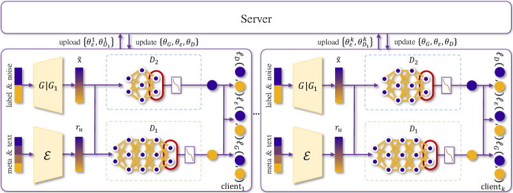
Figure 2. The proposed FedACK framework.

As shown in Fig. 2, FedACK consists of cross-lingual mapping, backbone model, and federated adversarial contrastive KD.

3.1. Cross-Lingual Mapping

We adopt a Transformer encoder-decoder-based method to achieve the alignment of different language contents. In essence, given a $m$-word text $x=\{x_{1},...,x_{m}\}$ in one language and the corresponding $n$-word text $y=\{y_{1},...,y_{n}\}$ in another language, we use an Encoder $\phi_{E}$ to transform the source text $x$ and the target text $y$ into context representations $z_{x}=\{z_{x_{1}},...,z_{x_{m}}\}$ and $z_{y}=\{z_{y_{1}},...,z_{y_{n}}\}$. We devise a Mapper $\mathcal{M}$ for converting between two context representation spaces, i.e., ${z_{x}}^{\prime}=\mathcal{M}(z_{y})$ and ${z_{y}}^{\prime}=\mathcal{M}(z_{x})$.

We introduce an adversarial mechanism for optimizing $\mathcal{M}$ so that the original $z_{x}$ and the mapped ${z_{x}}^{\prime}$ can be sufficiently similar. We first obtain the embedding of the context representations:

(2) $$\bar{z}_{x}=\frac{1}{m}\sum\limits_{k=1}^{m}{z_{x_{k}}},{\bar{z}_{x}}^{\prime}=\frac{1}{n}\sum\limits_{k=1}^{n}{z_{x_{k}}^{\prime}}.$$

Then we use the discriminator $D$ to distinguish whether an embedding $\bar{z}_{x}$ or ${\bar{z}_{x}}^{\prime}$ is forward propagated from $\mathcal{M}$ ($\bar{z}_{y}$ is equal to ${\bar{z}_{y}}^{\prime}$). Accordingly, the loss of the discriminator is defined as:

(3) $$\mathcal{L}_{dis}=\mathcal{L}_{dis_{x}}+\mathcal{L}_{dis_{y}},$$

$$\mathcal{L}_{dis_{x}}= {(D(\bar{z}_{x})-y_{\bar{z}_{x}})^{2}+(D({\bar{z}_{x}}^{\prime})-y_{{\bar{z}_{x}}^{\prime}})^{2}},$$

where the label $y_{\bar{z}}$ is set as 0 if an embedding $\bar{z}$ is mapped from $\mathcal{M}$. We combine the encoder $\phi_{E}$ and the mapper $\mathcal{M}$ into the generator. Similarly, the loss of the generator is:

(4) $$\mathcal{L}_{gen}=(D({\bar{z}_{x}}^{\prime})-y_{{\bar{z}_{x}}^{\prime}})^{2}+(D({\bar{z}_{y}}^{\prime})-y_{{\bar{z}_{y}}^{\prime}})^{2},$$

where the label $y_{\bar{z}}$ is always set as 1 to produce sufficiently similar representations to confuse the discriminator. We collect the context representations $(z_{x},z_{y},{z_{x}}^{\prime},{z_{y}}^{\prime})$ and decode them with a Decoder $\phi_{D}$ and generate the corresponding translation $(\tilde{z}_{y},\tilde{z}_{x},{\tilde{z}_{y}}^{\prime},{\tilde{z}_{x}}^{\prime})$, where $\tilde{z}_{y}=\phi_{D}(z_{x})$ and other terms are calculated in a similar way.

The loss of the Transformer is therefore defined as the cross-entropy loss between $x$ and $y$:

(5) $$\mathcal{L}_{trans}=\mathcal{L}_{z_{x}}+\mathcal{L}_{z_{y}}+\mathcal{L}_{{z_{x}}^{\prime}}+\mathcal{L}_{{z_{y}}^{\prime}},$$

$$\mathcal{L}_{z_{x}}=-\sum\limits_{t=1}^{n}\log P(y_{t}|\tilde{z}_{y}<t,z_{x}),$$

$$\mathcal{L}_{{z_{x}}^{\prime}}=-\sum\limits_{t=1}^{n}\log P(y_{t}|{\tilde{z}_{y}}^{\prime}<t,{z_{x}}^{\prime}).$$

3.2. Backbone Model for Feature Extraction

The main task is to let user-level backbone feature extractor model $\varepsilon$ to extract features per user metadata (e.g., account properties) and textual data (e.g., tweets). We concatenate the key items extracted from the metadata into the property vector $u_{p}$, following the similar way as (Yang et al., 2020, 2022), which is converted into user’s property representation $r_{p}$ by a Multi-layer Perceptron $r_{p}=MLP(u_{p})$. For textual data, assume a user has posted M Tweets $u_{t}=\{t_{1}^{1},\dots,t_{Q_{1}}^{1},t_{1}^{2},\dots,t_{Q_{M}}^{M}\}$, possibly in the form of different languages; $t^{j}_{i}$ represents the $i$-th word in the $j$-th tweet. We leverage the Encoder and Mapper delivered by the aforementioned cross-lingual module to convert each $u_{t}$ into a uniformed contextual space, i.e., $z_{u_{t}}=\{z_{1}^{1},\dots,z_{Q_{1}}^{1},{z_{1}^{2}}^{\prime},\dots,z_{Q_{M}}^{M}\}$. A Convolutional Neural Networks (CNN) layer, i.e., TextCNN(Kim, 2014), is then used to obtain the tweet-level representation $h_{u_{t}}$:

(6) $$h_{u_{t}}=\{h_{1}^{t},\dots,h_{M}^{t}\},h_{j}^{t}=CNN(\{z_{1}^{j},\dots,z_{Q_{1}}^{j}\}).$$

An attention layer is used to quantify the influence of each tweet on the overall semantics of the user and to calculate the user-level tweet representation $r_{t}$ through weighted aggregation of all tweets. The complete user-level representation $r_{u}$ is:

(7) $$r_{u}=MLP(concat(r_{p},r_{t})).$$

3.3. Federated Adversarial Contrastive KD

Architecturally, we follow the conventional server-client design for the Federated GAN-based KD. A client $k$ contains a global generator $G$ for KD, and a local generator $G_{k}$ for data enhancement. We use two discriminators – $D_{1}$ shared across all clients with the same architecture and initial parameters but trained on local data, and $D_{2}$ exclusively designated for each client to satisfy its individual demand. Each client uses a backbone model $\varepsilon$ to get the user’s representation $r_{u}=\varepsilon(x_{u})$ from local data $\mathcal{D}_{k}$. As a significant departure from the state-of-the-arts, a new multi-stage adversarial mechanism is proposed for jointly optimizing classification in both discriminators at intra-client level and a contrastive mechanism for aligning different feature spaces across clients. The notations are detailed in Appendix A.1.

3.3.1. Local Adversarial Contrastive KD

The adversarial learning on a per client basis include the following multi-phases.

Stage-1: Training D1 and D2 as classifiers. We aim to facilitate the two models to learn different decision boundaries for the same class of samples and compress the feature space of the feature extractor. To tackle non-IID data distribution and data scarcity among clients, we treat the shared global generator $G$ as teacher network and distill the knowledge of global data distribution from it. For each sample $(x^{k}_{i},y^{k}_{i})$, $G$ uses a standard Gaussian noise $z\sim\mathcal{N}(0,1)$ and label $y^{k}_{i}$ to generate pseudo-data $\tilde{x}=G(z,y^{k}_{i};\theta_{G})$. $(x^{k}_{i},\tilde{x})$ is fed into $D_{1}$ to obtain the probability distributions $(p,\tilde{p})$. We make $D_{1}$ fit probability $p$ of real data $x^{k}_{i}$ close to $\tilde{p}$ to distill knowledge by minimizing Eq. (8):

(8) $$\vspace{-0.4em}\mathcal{L}^{k}_{dis}=\frac{1}{N_{k}}\sum\limits^{N_{k}}_{i=1}D_{KL}(\sigma(D_{1}(r^{k}_{i}))||\sigma(D_{1}(\tilde{x})),\vspace{-0.2em}$$

where $\sigma$ is the softmax function, $D_{KL}$ is the Kullback–Leibler divergence and $r^{k}_{i}=\varepsilon(x^{k}_{i})$. Similar ${\mathcal{L}^{k}_{dis}}^{\prime}$ is performed for $D_{2}$.

We induce an adversarial loss to measure the probability difference between $D_{1}$ and $D_{2}$:

(9) $$\mathcal{L}^{k}_{adv}=\frac{1}{N_{k}}\sum\limits^{N_{k}}_{i=1}D_{KL}(\sigma(D_{1}(r^{k}_{i}))||\sigma(D_{2}(r^{k}_{i}))).$$

In essence, maximizing Eq. (9) can produce distinct decision boundaries between two discriminators to compress overlapping decision space. Intuitively, this is because $\varepsilon$ would learn more precise feature space if the representations could be correctly classified by both discriminators. Similarly to Eq. (9), we calculate adversarial loss $\mathcal{L}^{k}_{advg}$ on the pseudo-data generated by the local generator $G_{k}$ and minimize it to intensify the above process. $D_{1}$ and $D_{2}$ also need to correctly classify the pseudo-data randomly generated by $G$ to deal with the issue of unbalanced and scarce data. To sum up, the overall loss function of the discriminators is:

(10) $$\mathcal{L}^{k}_{D}=\mathcal{L}^{k}_{cls}+\alpha(\mathcal{L}^{k}_{dis}+{\mathcal{L}^{k}_{dis}}^{\prime})+\gamma(\mathcal{L}^{k}_{advg}-\mathcal{L}^{k}_{adv}).$$

Stage-2: Training $\varepsilon$. We minimize the adversarial loss Eq. (9) to reduce the difference between the probability outputs of two discriminators for the same feature. This means that the same data point can fall on the same side of the decision boundaries of the two discriminators. The feature space of the feature extractor is compressed and enforced to generate more precise features.

We use contrastive learning to navigate the optimization direction of feature extractor, thereby overcoming the model drift between local extractors and the global extractor. We expect the newly optimized $\varepsilon^{k}_{t}$ to produce a representation $r=\varepsilon^{k}_{t}(x^{k}_{i})$ as close as possible to the $r_{glo}=\varepsilon_{t}(x^{k}_{i})$ generated by the global extractor $\varepsilon$ while as far away as possible from the last round result of the feature extractor $r_{pre}=\varepsilon_{t-1}(x^{k}_{i})$. We define the following contrastive loss function:

(11) $$\mathcal{L}^{k,i}_{con}=-\log\frac{\exp({\rm sim}(r,r_{glo})/\tau)}{\exp({\rm sim}(r,r_{glo})/\tau)+\exp({\rm sim}(r,r_{pre})/\tau)},$$

where sim is the similarity measure function and $\tau$ denotes a temperature parameter. This can not only reduce the local models’ drift but also serve as a bridge with adversarial learning to make models of different clients have a consistent feature space. The loss function extractor is defined as follows:

(12) $$\vspace{-0.2em}\mathcal{L}^{k}_{\varepsilon}=\mathcal{L}^{k}_{cls}+\gamma\mathcal{L}^{k}_{adv}+\mu\frac{1}{N_{k}}\sum\limits^{N_{k}}_{i=1}\mathcal{L}^{k,i}_{con}.\vspace{-0.2em}$$

Stage-3: Training $G_{k}$. We maximize $\mathcal{L}^{k}_{advg}$ to ensure $G_{k}$ can generate pseudo-data that falls near the decision boundaries of two discriminators. This enforces such boundaries closer to the coincidence region, which further compresses the consistent feature space of the $\varepsilon$. As $G_{k}$ only generates the same data for each class, we add the diversity loss $\mathcal{L}_{var}$ to improve the diversity of the generated data and prevent model collapse:

(13) $$\mathcal{L}_{var}=e^{\frac{1}{N*N}\sum\limits_{i,j\in\{1,\cdots,N\}}(-\parallel\tilde{x}_{i}-\tilde{x}_{j}\parallel_{2}*\parallel z_{i}-z_{j}\parallel_{2})},$$

where $\tilde{x}_{i}=G_{k}(z_{i},\hat{y}_{i})$. The overall loss for generator $G_{k}$ can be calculated through:

(14) $$\mathcal{L}^{k}_{g}=\mathcal{L}^{k}_{cls}-\mathcal{L}^{k}_{advg}+\mathcal{L}_{var}.$$

3.3.2. Server Aggregation Knowledge Extraction

In each communication round, the client $k$ uploads the local parameters of $\{\theta^{k}_{\varepsilon},\theta^{k}_{D_{1}}\}$ to the server once the local training is finished, then waits for the updated global $G$, $D$ and $\varepsilon$ from the server to start a new round of local training. Once the server receives the latest parameters of the participating clients, it performs the model aggregation by weighted average and gets the updated global $\varepsilon$ and $D$:

(15) $$\theta_{\varepsilon}=\sum^{M}_{k=1}\frac{\parallel\mathcal{D}_{k}\parallel}{\parallel\mathcal{D}\parallel}\theta^{k}_{\varepsilon},\theta_{D}=\sum^{M}_{k=1}\frac{\parallel\mathcal{D}_{k}\parallel}{\parallel\mathcal{D}\parallel}\theta^{k}_{D_{1}},$$

where $M$ is the number of participating clients.

To ensure global data distribution can adapt to local distributions that may largely drift from each other, we exploit the global discriminator $D$ and global generator $G$ for global knowledge extraction, without a need for server-side KD using proxy data. client’s $D_{1}$ is used as the teacher network and define the loss of $G$ as:

(16) $$\mathcal{L}_{G}=\frac{1}{K}\sum^{K}_{k=1}\sum_{\tilde{x}}\alpha^{k,y}_{t}[D_{KL}\left(\sigma(D^{k}_{1}(\tilde{x}))||\sigma(D(\tilde{x}))\right)+\mathcal{L}^{\tilde{x}}_{cls}],$$

where $\tilde{x}$ is from empirical samples $\mathcal{D}_{G}$ generated by $G$ using noise $z\sim\mathcal{N}(0,1)$ and label $y\sim p(y)$. $\alpha^{k,y}_{t}$ is the ratio of samples with label $y$ stored in client $k$ against the same label samples in $\mathcal{D}$. $p(y)$ is obtained by label counts from clients through communication.

3.4. Pipeline of FedACK

Alg. 1 summarizes the overall pipeline of FedACK. The cross-lingual model $\phi_{E}$ and $\mathcal{M}$ for the backbone model $\varepsilon$ are first trained on the server (Line 1) and distributed to all clients. In each communication round, FedACK first broadcasts the up-to-date $G$, $\varepsilon$ and $D$ to a selected subset of clients $S_{t}$ (Line 1). Each client optimizes all the required models $D^{k}_{1},D^{k}_{2}$, $\varepsilon$ and $G_{k}$ using local data (Lines 1-1). When the parallel optimization completes, the server aggregates the clients’ parameters in this round to update the global parameters $\theta_{\varepsilon},\theta_{D}$ and to optimize the global generator $G$ (Lines 1-1).

Input: Local data $\mathcal{D}_{k}$, $k=1,\cdots,K$, corpus data $\mathcal{D}_{c}$, models $G_{k}$, $\phi_{E}$, $\mathcal{M}$, $\varepsilon$, $D^{k}_{1}$, $D^{k}_{2}$, $G$, $D$

Output: Local model $D_{2}$, global models $\phi_{E}$, $\mathcal{M}$, $\varepsilon$, $G$

1 initialization;

2 Server trains $\phi_{E}$, $\mathcal{M}$ via Eq.(5) based on $\mathcal{D}_{c}$, and transfers $\theta_{\phi_{E}}$, $\theta_{\mathcal{M}}$ to clients;

3 for each communication round $t=1,\ldots,T$ do

4      

5      $S_{t}\leftarrow$ random subset ($C$ fraction) of the $K$ clients;

6       Server broadcasts $\{\theta_{G},\theta_{\varepsilon},\theta_{D}\}$ to $S_{t}$ ;

7       for each client $k\in S_{t}$ in parallel do

8             Client $k$ updates $\{\theta_{G},\theta^{k}_{\varepsilon},\theta^{k}_{D_{1}}\}$ ;

9             for each local epoch $e=1,\cdots,E$  do

10                   calculate $\mathcal{L}^{k}_{D}$ via Eq.(10) ;

11                   {$\theta^{k}_{D_{1}},\theta^{k}_{D_{2}}\}\leftarrow\{\theta^{k}_{D_{1}},\theta^{k}_{D_{2}}\}-\nabla\mathcal{L}^{k}_{D}$;

12                  

13             end for

14            for each local epoch $e=1,\cdots,E$  do

15                   calculate $\mathcal{L}^{k}_{\varepsilon}$ via Eq.(12), $\theta^{k}_{\varepsilon}\leftarrow\theta^{k}_{\varepsilon}-\nabla\mathcal{L}^{k}_{\varepsilon}$;

16                  

17             end for

18            for each local epoch $e=1,\cdots,E$  do

19                   calculate $\mathcal{L}^{k}_{g}$ via Eq.(14), $\theta^{k}_{G_{k}}\leftarrow\theta^{k}_{G_{k}}-\nabla\mathcal{L}^{k}_{g}$;

20                  

21             end for

22             Client $k$ sends $\{\theta^{k}_{\varepsilon},\theta^{k}_{D_{1}}\}$ back to server;

23            

24       end for

25      Server update $\{\theta_{\varepsilon},\theta_{D}\}\leftarrow$ Eq.(15) ;

26       Server calculate $\mathcal{L}_{G}$ for $G$ via Eq.(16) ;

27       $\theta_{G}\leftarrow\theta_{G}-\nabla\mathcal{L}_{G}$

28 end for

Algorithm 1 FedACK

4. Evaluation

The experiments aim to answer the following questions:

• Q1. How does FedACK perform in classification under different data distribution scenarios?

• Q2. How does FedACK perform in learning efficiency?

• Q3. Can FedACK learn consistent feature space across clients?

• Q4. What is the effect of the different parameter values in different stages of FedACK?

• Q5. How does the cross-lingual module perform when combined FedACK and other baselines?

4.1. Experimental Setup

4.1.1. Software and Hardware

FedACK is implemented with Python 3.8.10, Pytorch 1.7.1 and runs on two servers, one is equipped with NVIDIA Tesla V100 GPU, 2.20GHz Intel Xeon Gold 5220 CPU and 512GB RAM, and the other is equipped with NVIDIA GeForce RTX 3090 GPU, 3.40GHz Intel Xeon Gold 6246 CPU and 256GB RAM.

4.1.2. Datasets

We conduct experiments on two Twitter bot datasets Vendor-19 (Yang et al., 2019) and TwiBot-20 (Feng et al., 2021b), the largest ones in the public domain by far. We mix the Vendor-19 with a dataset of benign accounts Verified which is presented in (Yang et al., 2020). The newly released TwiBot-20 dataset exposes users’ social relationships and enables the use of advanced graph representation-based algorithms. More dataset statistics are outlined in Appendix A.2.

4.1.3. Data heterogeneity

We use Dirichlet Distribution Dir ($\alpha$) to mock the non-IID given in (Li et al., 2021a) and split the bot dataset with heterogeneity. $\alpha$ is an indicator of Dirichlet distribution – the smaller $\alpha$ is, the more heterogeneous the data distribution is.

4.1.4. Baselines

As federated KD provided a natural pathway to privacy preservation without sharing original data – the key concern in cross-platform bot detection – federated KD-based approaches baselines that can handle heterogeneity of non-IID data are the pedestal focus of the comparison. FedAvg and (McMahan et al., 2017), FedProx (Li et al., 2020) improve the local model training and update under heterogeneity through adding an optimization item. FedDF (Lin et al., 2020) employs data-free knowledge distillation to improve the global model on server side. FedEnsemble (Shi et al., 2021) uses an ensemble mechanism for combining the output of all models to predict a specific sample. FedDistill (Shi et al., 2021) shares label-wise average of logit vectors among users for data-free knowledge distillation without network parameter shared. FedGen (Zhu et al., 2021) and FedFTG (Zhang et al., 2022) offer flexible parameter sharing and knowledge distillation.

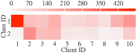
(a) Vendor-19 ($\alpha=1$).

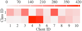
(b) Vendor-19 ($\alpha=0.5$).

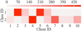
(c) Vendor-19 ($\alpha=0.1$).

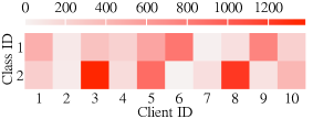
(d) TwiBot-20 ($\alpha=1$).

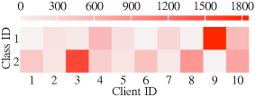
(e) TwiBot-20 ($\alpha=0.5$).

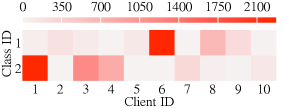
(f) TwiBot-20 ($\alpha=0.1$).

Figure 3. Visualization of data heterogeneity. The darker color means more training samples with a label available to the client.

Table 1. Comparison of the average maximum accuracy of different methods for social bot detection (%).

Dataset	Vendor-19				TwiBot-20
Setting	$\alpha=1$	$\alpha=0.5$	$\alpha=0.1$	$\alpha=0.05$	$\alpha=1$	$\alpha=0.5$	$\alpha=0.1$	$\alpha=0.05$
FedAvg	71.30$\pm$0.60	61.06$\pm$1.52	60.88$\pm$2.85	59.81$\pm$2.48	54.04$\pm$0.50	55.41$\pm$1.35	51.37$\pm$0.77	52.46$\pm$0.02
FedProx	84.37$\pm$0.43	78.25$\pm$1.02	51.86$\pm$0.04	63.27$\pm$2.32	74.34$\pm$0.06	73.32$\pm$0.25	51.86$\pm$0.04	52.30$\pm$0.63
FedDF	86.37$\pm$1.23	80.17$\pm$2.21	63.16$\pm$1.37	67.01$\pm$1.78	72.12$\pm$1.96	71.25$\pm$1.03	55.23$\pm$1.32	53.35$\pm$1.41
FedEnsemble	81.12$\pm$2.22	76.70$\pm$1.21	64.51$\pm$2.56	68.05$\pm$1.15	55.98$\pm$2.55	54.15$\pm$0.04	54.21$\pm$0.04	54.15$\pm$0.04
FedDistill	79.68$\pm$0.58	68.77$\pm$1.13	52.88$\pm$0.06	70.25$\pm$0.39	64.11$\pm$0.29	63.34$\pm$0.56	50.00$\pm$0.00	54.30$\pm$0.05
FedGen	90.05$\pm$0.33	84.83$\pm$0.96	65.12$\pm$0.60	70.79$\pm$2.39	74.14$\pm$0.47	73.12$\pm$2.09	59.19$\pm$2.70	55.78$\pm$1.79
FedFTG	88.31$\pm$1.41	82.17$\pm$1.52	66.01$\pm$1.25	68.39$\pm$1.94	74.27$\pm$1.21	74.13$\pm$0.53	60.14 $\pm$1.74	56.17$\pm$1.27
FedACK-A	91.31$\pm$0.52	84.79$\pm$1.05	66.10$\pm$2.90	68.21$\pm$1.95	77.16$\pm$1.09	74.70$\pm$1.64	63.52$\pm$1.09	55.39$\pm$1.24
FedACK	88.58$\pm$1.91	87.05$\pm$2.03	76.04$\pm$3.40	75.27$\pm$2.50	77.08$\pm$1.83	78.26$\pm$2.60	67.81$\pm$2.20	60.14$\pm$1.32
Gain	$\uparrow$ 1.26$\sim$20.01	$\uparrow$ 2.22$\sim$25.99	$\uparrow$ 10.03$\sim$24.18	$\uparrow$ 4.48$\sim$15.46	$\uparrow$ 2.82$\sim$23.12	$\uparrow$ 4.13$\sim$24.11	$\uparrow$ 7.67$\sim$16.44	$\uparrow$ 3.97$\sim$7.84

4.1.5. Model Parameters

The cross-lingual module is trained upon the corpus released in (Zhu et al., 2019). To be fair, the same cross-lingual module and backbone model $\varepsilon$ (same architecture and initial parameters) are used upon all baseline approaches. For the transformer architectures in the cross-lingual module, we use the same configuration of (Vaswani et al., 2017); the number of layers, feed-forward hidden size, model hidden size and the number of heads are 6, 1024, 512, and 8, respectively. The mapper is an MLP with three linear layers with a hidden dimension of 512, and the discriminator is an MLP with four linear layers with a hidden dimension of 512. The MLP used for extracting property features in the backbone model has two linear layers with a hidden dimension of 512. TextCNN (Kim, 2014) used in $\varepsilon$ has four convolution kernels of size [2, 3, 4, 5]. The generators in FedACK are MLP with two linear layers with a hidden dimension of 256. The discriminators in FedACK are MLP with 3 linear layers with a hidden dimension of 256. Common parameters for training the models include: batch size (64), learning rate (0.01), optimizer (Adam), global communication rounds (100), and local updating steps (5).

4.1.6. Methodology and Metrics

The comparison is five-fold: 1) effectiveness (model accuracy and capability of handling heterogeneity), 2) efficiency (the number of communication rounds required to achieve a target accuracy) and 3) the effect of learning consistent feature space. 4) sensitivity (variation of model accuracy under different hyperparameter settings) 5) cross-lingual validation (performance gains of our proposed cross-lingual modules in cross-platform scenarios where multiple languages coexist). Since the samples of different categories in the datasets are balanced, we simply use accuracy and deviation as the main metrics.

4.2. Effectiveness (Q1)

We vary the hyperparameter dataset partition $\alpha$ from $\{1,0.5,0.1,0.05\}$ for each dataset to validate the performance of different methods with varying degrees of data distribution heterogeneity. The darkness of coloring represents the sample number of a specific class stored on a client. As shown in Fig. 3, increased data heterogeneity (e.g., $\alpha=0.1$) leads to more clients store only one class of samples.

Accuracy Comparison. Table 1 compares the accuracy among baseline algorithms. All experiments are repeated over 3 random seeds. Overall, our method outperforms all baselines in any scenario. FedACK achieves 1.26%$\sim$10.03% accuracy improvement in absolute terms when compared with the runner-up methods (i.e., FedGen, FedFTG). While FedProx can achieve relatively competitive performance when data heterogeneity is less intense (e.g., $\alpha=\{1,0.5\}$) due to its limit to local model updates, it cannot well handle more heterogeneous data distribution. The data-free knowledge distillation in FedGen and FedFTG can substantially improve the server’s global model; however, they are insufficient to effectively tackle feature space inconsistency and model drift. The performance gain FedACK is more significant against other baselines when data heterogeneity increases (e.g., $\alpha=\{0.1,0.05\}$), indicating its superiority in handling data heterogeneity. Appendix A.3 further demonstrates the improved model generalization in our approach when compared with other baselines.

Ablation Study. We generated a new variant model, FedACK-A, that excludes the contrastive module. As shown in Table 1, the accuracy of FedACK-A is outstanding when data heterogeneity is low but falls off when higher heterogeneity manifests. This indicates the adversarial training and global knowledge distillation alone can function effectively in the face of low heterogeneity. The contrastive learning mechanism is of importance to constrain the model optimization direction, which demonstrate the necessity of learning consistent feature spaces when dealing with data heterogeneity.

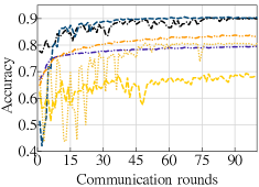
(a) Vendor-19 ($\alpha=1$).

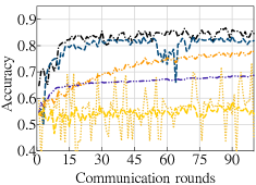
(b) Vendor-19 ($\alpha=0.5$).

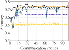
(c) TwiBot-20 ($\alpha=1$).

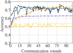
(d) TwiBot-20 ($\alpha=0.5$).

Figure 4. Learning Curve of (a-b) Vendor-19 and (c-d) TwiBot-20 in 100 communication rounds in different $\alpha$ settings.

Table 2. The round number to reach the target accuracy on Vendor-19 $(80\%,70\%)$ and TwiBot-20 $(70\%,65\%)$.

Dataset	Vendor-19		TwiBot-20
Setting	$\alpha=1\ (80)$	$\alpha=0.5\ (70)$	$\alpha=1\ (70)$	$\alpha=0.5\ (65)$
FedAvg	unreached	unreached	unreached	unreached
FedProx	25.3$\pm$3.1	32.6$\pm$2.3	13.3$\pm$2.8	24.0$\pm$7.3
FedDF	22.3$\pm$2.4	38.4$\pm$3.1	50.3$\pm$5.2	60.2$\pm$6.4
Ensemble	9.0$\pm$1.1	6.0$\pm$1.4	unreached	unreached
FedDistill	60.0$\pm$1.0	unreached	unreached	unreached
FedGen	7.3$\pm$0.4	5.0$\pm$0.8	10.6$\pm$0.9	4.6$\pm$1.2
FedFTG	43.5$\pm$37.5	15.6$\pm$16.5	12.6$\pm$0.5	9.4$\pm$2.3
FedACK	4.6$\pm$3.8	2.3$\pm$0.9	2.33$\pm$1.25	1.67$\pm$0.94

4.3. Efficiency (Q2)

Fig. 4 shows the learning curve of different methods within 100 communication rounds and FedACK is among the top performers. FedDistill has the best stability, rapidly approaching a stable level only after a dozen rounds of communication, but the achievable accuracy is merely lower than 0.65, making it less competitive when compared with other methods. FedACK can very quickly converge to a high level of accuracy after the initial rounds and remains high in the following communication rounds.

Table 2 reports the average number of rounds required for each method to achieve the target accuracy in different settings. Unreached means the failure of achieving the target accuracy ($80\%,70\%$ for Vendor-19; $70\%,65\%$ for TwiBot-20) in all three runs with different random seed. FedACK achieves target accuracy with a minimum number of communication rounds under any circumstance. FedGen, the second best performer, still requires 1.6$\sim$4.5 times the communication rounds of our method. This is because FedACK incorporates the proportion of the label of each pseudo sample in each client into a part of knowledge during global knowledge extraction and classification. This indicates the importance of each client to the knowledge of a specific sample. FedACK also limits the feature space and optimization direction of the models at the client side, resulting in quicker convergence to target a given accuracy.

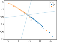
(a) Visualization of client 1.

(b) Visualization of client 2.

Figure 5. Decision boundaries and feature space of two randomly selected clients from FedACK trained on Vendor-19. The x-axis and y-axis represent the values of the 2-dimensional features output by $\varepsilon$ described in Sec 4.4.

4.4. Feature Space Consistency (Q3)

We also conduct an experiment to show how FedACK learns the feature space. Fig. 5 visualizes the learnt feature space and the decision boundaries of two classifiers in FedACK on Vendor-19 dataset. We tweak the feature extractor $\varepsilon$ to produce 2-dimension features for each input sample. We randomly select two clients after training FedACK in 100 communication rounds and plot the features of testing data samples. It can be observed that adversarial learning makes the two classifiers in any of the two clients learn distinct decision boundaries. The different decision boundaries impose restrictions on the feature space learned by the feature extractor. To extract features from the same class of samples and locate them in overlapping areas on the same side of the decision boundary, the feature extractor compresses the generated features into a linear region for simultaneous classification. Another observation on Fig. 5(a) and Fig. 5(b) is that the feature extractors learn a consistent feature space across clients due to the contrastive learning that limits the update direction of the feature extractors. These findings show the advancements of FedACK in learning feature spaces.

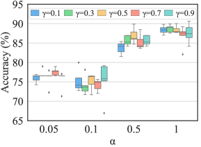
(a) FedACK with different $\gamma$ in adversarial learning.

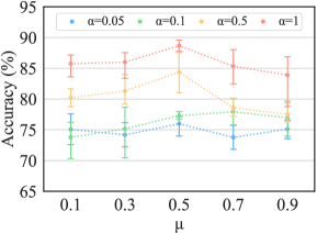
(b) FedACK with different $\mu$ in contrastive learning.

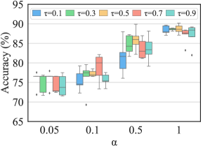
(c) FedACK with different $\tau$ in contrastive learning.

Figure 6. Hyperparameter Sensitivity ($\gamma,\mu,\tau$) of FedACK (a-c) on Vendor-19 under different data heterogeneity settings ($\alpha$).

4.5. Sensitivity (Q4)

We investigate the hyper-parameters sensitivity based on the Vendor-19 dataset. The hyperparameters include $\gamma$ for adjusting the proportion of adversarial loss, and $\mu$ and $\tau$ for adjusting the proportion of contrastive loss. The number of repeated random seeds is set as 5.

As shown in Fig. 6(a), when the heterogeneity of data distribution is marginal (i.e., $\alpha=1$), the accuracy is insensitive to $\gamma$. However, when the heterogeneity increases (i.e., $\alpha$ going down), noticeable accuracy variation manifests among different settings of $\gamma$. Similar observations can be found in Fig. 6(c), indicating a discrepancy in the accuracy among different $\tau$. These findings implicate a great need for carefully examining and fine-tuning such parameters in the adversarial and contrastive loss on a case-by-case basis, considering the data characteristics (particularly the heterogeneity of data distribution), to target the optimal model performance. Fig 6(b) depicts the accuracy under different combinations of $\mu$ and $\alpha$. Observably, for a given data distribution, the model accuracy reaches its peak when $\mu$ increases to 0.5, before falling off if $\mu$ continues to increase. This is largely due to a balance between adversarial loss and contrastive loss. The dominance of either side will lead to a degradation of the model’s effectiveness.

4.6. Cross-Lingual Validation (Q5)

As there is no publicly available datasets in the field of social bot detection designated for cross-lingual performance at the time of writing, we synthesize an experimental cross-lingual dataset by randomly selecting half the social accounts from Vendor-19 dataset and translating their tweets into Chinese using Google Translate. We use the same experiment settings described in Section 4.1. We pre-train the cross-lingual mapper by using the cross-lingual summarization corpus NCLS (Zhu et al., 2019) and then combine the pre-trained encoder $\phi_{E}$ and mapper $\mathcal{M}$ with FedACK and other baselines. By default, each method is evaluated with the cross-lingual mapper $\mathcal{M}$ enabled. Each method with the suffix -NC means the model only uses $\phi_{E}$ to extract features from text content without $\mathcal{M}$.

Experimental results are shown in Table 3. The observations are three-fold: i) FedACK constantly outperforms others in all circumstances. The accuracy can increase 3.28$\sim$6.45 in absolute value, when data heterogeneity is low ($\alpha=1$). ii) Compared with the model variant without $\mathcal{M}$ (e.g. FedACK-NC), the accuracy of the model (e.g. FedACK) equipped with the cross-lingual mapper is unsurprisingly improved. This once again demonstrates the substantial capability and necessity of coping with cross-lingual issues. It is worth noting that there is also a diminishing performance gain from cross-language mapping as the $\alpha$ value gets smaller. This is because the heterogeneity of data distribution becomes the dominating challenge to accuracy, and the cross-lingual module itself is insufficient and thus brings limited benefit. iii) Equipped with the cross-lingual mapper, each method can well tackle the multi-lingual scenarios. There is marginal disparity between the model accuracy in the case of a singular language environment (shown in Table 1) and the accuracy when multiple languages co-exist in the tweet features (as shown in Table 3). This demonstrates the robustness and effectiveness of the proposed mapper for cross-lingual contents. Among all the comparative baselines, our method has the least degradation caused by the existence of multiple languages, owing to the unified feature space mapping for different languages.

Table 3. Comparison of the average maximum accuracy (%) of different methods with/without(-NC) cross-lingual mapping. Gain is the disparity between FedACK and other baselines.

Dataset	Vendor-19
Setting	$\alpha=1$	$\alpha=0.5$	$\alpha=0.1$	$\alpha=0.05$
FedDistill-NC	78.14$\pm$1.30	67.01$\pm$0.16	66.35$\pm$0.25	69.24$\pm$0.30
FedDistill	80.03$\pm$0.59	68.87$\pm$0.30	67.20$\pm$0.22	70.18$\pm$0.45
FedGen-NC	81.94$\pm$0.82	77.88$\pm$0.52	70.65$\pm$2.73	72.73$\pm$2.20
FedGen	83.20$\pm$1.07	79.63$\pm$0.57	72.42$\pm$2.18	73.26$\pm$0.53
FedFTG-NC	78.18$\pm$1.04	76.79$\pm$1.22	67.61$\pm$1.57	72.30$\pm$1.20
FedFTG	82.85$\pm$1.52	77.29$\pm$3.42	69.65$\pm$0.95	73.15$\pm$1.27
FedACK-NC	84.54$\pm$1.30	79.37$\pm$1.24	73.99$\pm$2.55	74.48$\pm$ 1.50
FedACK	86.48$\pm$0.99	81.16$\pm$1.06	75.05$\pm$2.78	74.18$\pm$1.67
Gain	$\uparrow$ 3.28$\sim$6.45	$\uparrow$ 1.53$\sim$12.29	$\uparrow$ 2.63$\sim$7.85	$\uparrow$ 0.92$\sim$4.0

5. Conclusion

Social bots have been growing in the social media platforms for years. State-of-the-art bot detection methods fail to incorporate individual platforms with different models and data characteristics. In this paper, we devise a GAN-based federated knowledge distillation mechanism for efficiently transferring knowledge of data distribution among clients. We elaborate a contrast and adversarial learning method to ensure consistent feature space for better knowledge transfer and representation when tackling non-IID data and data scarcity among clients. Experiments show that FedACK outperforms baseline methods in terms of accuracy, learning efficiency, and feature space consistency. In the future, we will theoretically investigate the feature space consistency and extend FedACK to fit graph-based datasets with diversified entities and relations.

Appendix A Appendix

A.1. Glossary of Notations

In Table 4, we summarize the main notations used in this work.

Table 4. Notations.

Symbol	Definition
$\mathcal{L}$	Defined loss function
$K$; $N_{k}$	Number of clients; Number of samples in $k$-th client
$x_{m}$; $y_{n}$	The $m$-th word and $n$-th word in two different language contents
$\phi_{E}$	The encoder for text content representation
$\phi_{D}$	The decoder for translating context representation
$\mathcal{M}$	The cross-lingual mapper for converting context representation
$z_{x}$	Text context representation vector
$\epsilon$	The backbone model for user feature extraction
$u_{t}$	The tweets set from $t$-th user
$t^{m}_{i}$	The $i$-th word in user’s $m$-th tweet
$h^{t}_{m}$	Representation for $m$-th tweet posted by $t$-th user
$r_{p}$; $r_{t}$	User’s property representation; tweet-level representation
$r_{u}$,$r$	User-level representation
$G$; $D_{1}$, $D_{2}$	Generator; Discriminators
$\mathcal{D}_{k}$	The local data stored in the $k$-th client
$\mathcal{D}$	The data set collected from all clients
$(x^{k}_{i},y^{k}_{i})$	The $i$-th sample pair stored in the $k$-th client
$\mathcal{N}(0,1)$	The gaussian distribution
$\tilde{x}$	The pseudo-data generated by generators
$p$; $\hat{p}$	Probability of local data; Global data distribution probability
$D_{KL}$	The Kullback–Leibler divergence
$\tau$	The temperature parameter for smoothing similarity value
$\gamma,\mu$	The weight hyperparameter in the defined loss function
$\theta$	The parameters of the designed model
$M$	The number of clients participating in the communication
$\alpha^{k,y}_{t}$	Ratio of samples with label $y$ stored in ${client}_{k}$ against in $\mathcal{D}$

A.2. Statistics of Datasets

Table 5 summarizes the basic statistic information of datasets used in this work.

Table 5. Statistics of datasets.

Dataset	Humans	Bots	Total number
Vendor-19 (Yang et al., 2019)	1860	568	2428
TwiBot-20 (Feng et al., 2021b)	4175	5286	9461

A.3. Generalization Experiment

To validate the generalization of our method, we collected four additional public social bot detection datasets: Varol-17, Gilani-17, cresci-19, botometer-feedback-19. To simulate the scenario of bot detection in uniting multiple social platforms, we select one dataset from Vendor-19 and TwiBot-20 as the test dataset. Each of the remaining datasets is distributed to a specific client. In this circumstance, there are five clients and a server, and each client represents a social platform. We aim to demonstrate the enhanced model proposed in this work can still competitively detect new variants that have never been seen before, when all platforms share the characteristics of their own social bots with other platforms. As shown in Table 6, the difficulty detection in the two datasets is entirely different. For most of the approaches, the classification accuracy of TwiBot-20 dataset is merely 50%, which indicates a huge discrepancy of bot features among datasets. In other words, the detection models learnt from the early generations of bots can hardly detect the bots in TwiBot-20 in an accurate manner. By contrast, our approach can achieve a higher accuracy due to the ability to learn a consistent feature space; as a result, the bot account features in different clients can be effectively shared. Additionally, constraining the optimization direction of the client model can facilitate our model to obtain better representation ability, and hence a better generalization than others.

Table 6. Comparison of the average maximum accuracy of different methods which are tested on a specific dataset (Vendor-19 or TwiBot-20) and trained from the other datasets.

Test Dataset	Vendor-19	TwiBot-20
FedAvg	76.53$\pm$0.11	49.63$\pm$1.09
FedProx	74.26$\pm$3.57	54.21$\pm$2.01
Ensemble	76.01$\pm$0.65	51.98$\pm$5.50
FedDistill	73.11$\pm$0.95	51.19$\pm$1.12
FedGen	77.52$\pm$0.65	62.30$\pm$0.93
FedFTG	76.51$\pm$1.15	60.12$\pm$1.01
FedACK	78.13$\pm$1.38	64.79$\pm$1.61