Kernel Density Bayesian Inverse Reinforcement Learning

Abstract

Inverse reinforcement learning (IRL) infers an agent’s reward function using observed behavior. However, IRL algorithms that learn point estimates of the reward function may be misleading, as multiple reward functions often describe the agent’s behavior equally well. To address this limitation, a Bayesian approach to IRL models a distribution over candidate reward functions, introducing a strategy for representing the inherent uncertainty in the problem. Despite this improvement, several Bayesian IRL algorithms use a $Q$-value function as a component of the likelihood, which may result in irrational posterior updates and in computationally intensive posterior inference. To avoid these challenges, we propose kernel density Bayesian IRL (KD-BIRL), which approximates the likelihood using conditional kernel density estimation. Our approach provides an efficient and principled framework that can be applied to environments with complex and infinite state spaces. To illustrate its effectiveness, we conduct a series of experiments in Gridworld environments and a sepsis treatment task. Our results highlight KD-BIRL’s accuracy, particularly in low-data regimes.

Keywords Inverse reinforcement learning  $\cdot$ Bayesian statistics

1 Introduction

Reinforcement learning (RL) methods discover policies that maximize an agent’s long-term expected reward within a Markov decision process (MDP). In observational data settings, we observe sequences of states and actions as an agent follows policies optimizing for an unknown reward function. Learning the reward function can help identify the objectives driving the agent’s behavior. This reward function can also be used to replicate the agent’s behavior (imitation learning). We focus on inverse reinforcement learning (IRL) methods, which learn an agent’s reward function given observations of the agent’s behavior. These methods have been successfully applied across several domains, including robotics (Ratliff et al., 2006a; Kolter et al., 2008) and swarm animal movement (Ashwood et al., 2020).

The earliest IRL algorithms learned point estimates of a reward function that best explains an agent’s behavior (Abbeel and Ng, 2004; Ng and Russell, 2000); these algorithms were applied to problems in path planning (Mombaur et al., 2010), urban navigation (Ziebart et al., 2008) and robotics (Ratliff et al., 2006a; Kolter et al., 2008). A point estimate can be useful for imitation learning, where the inferred reward function is used to fit RL policies that replicate the desired behavior observed in expert demonstrations.

Despite the success of early IRL approaches, there are limitations to inferring a point estimate. First, the IRL problem is frequently nonidentifiable (Ziebart et al., 2008, 2009; Ratliff et al., 2006b; Abbeel and Ng, 2004), meaning there may be multiple (and possibly infinite) reward functions that explain a set of behaviors equally well. Second, for finite demonstration data, point estimates of the reward function fail to capture the uncertainty and noise in the data-generating process. Instead, a Bayesian approach, which treats the reward function as a draw from a distribution, can represent uncertainty. A Bayesian approach computes a posterior distribution that places mass on reward functions proportional to how well they explain the observed behavior (Ramachandran and Amir, 2007; Balakrishnan et al., 2020; Chan and van der Schaar, 2021; Michini and How, 2012a, b; Choi and Kim, 2012). Bayesian methods can be more useful for reward function analysis because they characterize the a posterior distribution on reward, which can highlight alternate explanations of agent objectives.

However, there are several issues with the likelihood approximation in existing Bayesian IRL methods. First, the use of a $Q$-value function in likelihood estimation is not guaranteed to result in rational posterior updates. Rational updates imply that higher likelihood for a given observation should translate to higher posterior probability. It cannot be assumed that a likelihood function parameterized using a $Q$-function satisfies all of the assumptions required for rational updates (details in Section 2.2 and Appendix 7).

Furthermore, in Bayesian modeling, likelihood specification has a large impact on the resulting posterior distribution. The true parametric family of the likelihood function (i.e., the probability of an observation given a reward function) is not given in the IRL setting. Existing approaches approximate the likelihood with a formulation that uses an optimal $Q$-value function (Ramachandran and Amir, 2007). A $Q$-value function estimates the long-term expected reward for a given observation and is learned using $Q$-learning (Sutton and Barto, 2018), a “forward RL” algorithm used to solve an MDP. The original algorithm pioneered by  Ramachandran and Amir (2007) and several of its successors use Markov chain Monte Carlo (MCMC) sampling to compute a posterior over the reward function, and every iteration of MCMC requires forward RL for a new sampled reward function. This is computationally expensive, especially with infinite or high-dimensional state spaces.

To avoid the issues surrounding using a $Q$-value function, we instead use kernel density estimation to approximate the data likelihood. The contributions of our work follow:

1. We propose KD-BIRL which uses conditional kernel density estimation to directly estimate the likelihood function leading to computationally tractable posterior inference (Section 3).

2. We justify our method theoretically by proving posterior consistency and demonstrating that the posterior contracts to the equivalence class of the expert reward function (Section 4).

3. With a feature-based reward function, KD-BIRL successfully infers a posterior over reward functions in complex state spaces, even in a low-data regime.

We first review fundamental topics and limitations of existing work in Section 2. Then, we formally introduce KD-BIRL in Section 3 and prove posterior consistency in Section 4. In Section 5, we demonstrate results in a Gridworld environment and a sepsis management task. Finally, in Section 6, we discuss broader implications and propose future research directions.

2 Preliminaries

2.1 Background

IRL methods infer an agent’s reward function given demonstrations of its behavior. An RL agent interacts with an environment defined using an MDP. An MDP is represented by $(\mathcal{S},\mathcal{A},P,R,\gamma)$, where $\mathcal{S}$ is the state space; $\mathcal{A}$ is a discrete set of actions; $P(\mathbf{s}_{t+1}|\mathbf{s}_{t},a_{t})$ defines state transition probabilities from time $t$ to $t+1$; $R:\mathcal{S}\rightarrow\mathbb{R}$ is a reward function, where $R\in\mathcal{R}$ and $\mathcal{R}$ denotes the space of reward functions; and $\gamma\in[0,1]$ is a constant and known discount factor. The input to an IRL algorithm is a set of $n$ expert demonstrations, $\{(s_{i}^{e},a_{i}^{e})\}_{i=1}^{n}$, where each demonstration is a $2$-tuple representing an $e$xpert agent’s state and chosen action. These demonstrations are assumed to arise from an agent acting optimally according to policy $\pi^{\star}:\mathcal{S}\rightarrow\mathcal{A}$. Given these expert demonstrations, IRL algorithms seek the fixed but unknown reward function $R^{\star}$ such that $\pi^{\star}$ is optimal with respect to $R^{\star}$.

Bayesian approaches to IRL treat the reward function $R$ as inherently random. By specifying a prior distribution over $R$ and a likelihood function for the observed data, these methods then infer a posterior distribution over $R$ given expert demonstrations. Using Bayes’ rule, the posterior density is equivalent to the product of the prior on the reward, $p(R)$, and the likelihood of the expert demonstrations given the reward function, with a normalizing constant that corresponds to the probability of the expert demonstrations:

$$p\left(R\,|\,\left\{(s_{i}^{e},a_{i}^{e})\right\}_{i=1}^{n}\right)=\frac{p(R)\prod_{i=1}^{n}p(s_{i}^{e},a_{i}^{e}|R)}{p(\left\{(s_{i}^{e},a_{i}^{e})\right\}_{i=1}^{n})}.$$ (1)

In the earliest formulation of Bayesian IRL (BIRL) (Ramachandran and Amir, 2007), the authors propose using a $Q$-value function to approximate the likelihood component of Equation 1. The $Q$-value function for a given policy $\pi$ at time $t$ is $Q^{\pi}(\mathbf{s}_{t},a_{t})=r(\mathbf{s}_{t},a_{t})+\gamma\mathbb{E}_{\mathbf{s}_{t+1}\sim P}[V^{\pi}(\mathbf{s}_{t+1})]$, where $s_{t}$, $a_{t}$, and $r_{t}$ are the state, action, and reward at time $t$, $r(s,a)$ is the reward function, and the value function of the policy is $V^{\pi}(\mathbf{s})=\mathbb{E}[\sum_{t=0}^{\infty}\gamma^{t}r_{t}|\mathbf{s}_{0}=\mathbf{s}]$. The aproach of Ramachandran and Amir (2007) uses an optimal $Q$-value function as a proxy for the likelihood within a Gibbs posterior framework. The likelihood takes the form

$$p(s,a\,|\,R)\propto e^{\alpha Q^{\star}(s,a,R)},$$ (2)

where $Q^{\star}(s,a,R)$ is the optimal $Q$-value function for reward function $R$, and $\alpha>0$ is an inverse temperature parameter.

There are several practical challenges associated with learning the aforementioned BIRL posterior. First, the optimal $Q^{\star}$ is found using $Q$-learning, and $Q^{\star}$ is typically expensive to estimate for a new $R$. BIRL uses MCMC, which requires learning a new $Q^{\star}$ for every $R$ sampled. Additionally, as we discuss in the next section, the use of $Q^{\star}$ in the likelihood is not guaranteed to result in rational posterior updates. This motivates us to avoid a $Q$-value function in the likelihood.

2.2 Potential irrationality of a Q-function based likelihood

Rational Bayesian updates imply that new evidence is used to update belief distributions in a Bayesian manner (i.e., the posterior satisfies Bayes rule). The consequences of producing irrational or invalid posterior updates are severe; irrational updates lead to a posterior that may not contract to the correct region of the parameter space. Using a $Q^{\star}$ in likelihood estimation, as many current approaches do, can certainly result in rational posterior updates, but this rationality must be verified, even if $Q^{\star}$ is a perfectly fit model; this verification is missing from existing Bayesian IRL literature. This rationality can be verified by checking to see if a given $Q$-value function satisfies the five assumptions for rational posterior updates posed in P. G. Bissiri (2016)(listed in Appendix 7).

One of the conditions for rational updates is that the likelihood of new evidence should be proportional to the posterior probability under the new evidence. It is possible for even a simple parameterization of $Q^{\star}$ to violate this assumption for some subset of the expert demonstrations. As an example, we evaluate a setting in which $Q^{\star}$ is a piece-wise linear function, and identify a combination of input data points $x,y$ in which the likelihood of observing $x$ is smaller than that of observing $y$, but the posterior probability is higher for $x$ than $y$, thus contradicting the assumption (Appendix 7). The difficulty of verifying these assumptions encourages us to use a kernel density estimator for the likelihood, which is a probability density function and thus satisfies all of the assumptions.

2.3 Related Work

Several extensions to the original BIRL algorithm (Ramachandran and Amir, 2007) have been proposed. One set of methods learn nonparametric reward functions (Levine et al., 2011; Qiao and Beling, 2011; Choi and Kim, 2013; Šošić et al., 2018; Choi and Kim, 2012). These algorithms use a variety of strategies such as Gaussian processes (Levine et al., 2011; Qiao and Beling, 2011), Indian buffet process (IBP) priors (Choi and Kim, 2013), and Dirichlet process mixture models (Choi and Kim, 2012) to learn reward functions for MDPs with large state spaces that may include sub-goals. Other methods reduce computational complexity by using either more informative priors (Rothkopf and Ballard, 2013), different sampling procedures (e.g., Metropolis-Hastings (Choi and Kim, 2012), expectation-maximization (Zheng et al., 2014)), variational inference (Chan and van der Schaar, 2021), or learning several reward functions that each describe a subset of the state space (Michini and How, 2012b, a). Despite the improvements, all of these approaches use a $Q$-value function in place of the likelihood and hence still may suffer from computational issues due to repetitive iterations of $Q$-learning, or may not result in rational posterior updates.

To address these issues within the confines of an IRL algorithm, it is necessary to either directly estimate the likelihood, or reduce the number of times forward RL is performed. Recent work proposes a variational Bayes framework, Approximate Variational Reward Imitation Learning (AVRIL) (Chan and van der Schaar, 2021), to approximate a posterior. This method improves upon existing work by avoiding re-estimating $Q^{\star}$ for every sampled reward function, allowing it to bypass some of the computational inefficiencies of Ramachandran and Amir (2007)’s initial formulation. However, AVRIL still requires the use of a $Q$-value function to approximate the likelihood, which is not guaranteed to result in rational posterior updates. Another method avoids using a $Q$-value function entirely for the likelihood (Michini et al., 2013) and instead approximates it using real-time dynamic programming or action comparison. This is best suited for environments with a closed-loop controller that provides instant feedback. To the best of our knowledge, no other work identifies or addresses the rationality issues posed by using $Q^{\star}$ in the likelihood estimate.

3 Method

3.1 Conditional kernel density estimation

Directly estimating the likelihood avoids the computational and rationality issues associated with using $Q^{\star}$. To estimate the likelihood $p(s,a\,|\,R)$, we first observe that it can be viewed as the conditional density of the state-action pair given the reward function. Thus, any appropriate conditional density estimator can be applied; examples include the conditional kernel density estimator (CKDE) (van der Vaart, 2000) and Gaussian processes. We adopt the CKDE because it is nonparametric, has a closed form, and is straightforward to implement (Holmes et al., 2007; Izbicki and Lee, 2016).

Motivated by the conditional probability equation $p(y|x)=\frac{p(x,y)}{p(x)},$ where $x$ and $y$ are two generic random variables, the CKDE estimates the conditional density $p(y|x)$ by approximating the joint distribution $p(x,y)$ and marginal distribution $p(x)$ separately via kernel density estimation (KDE). Given pairs of observations $\{(x_{j},y_{j})\}_{j=1}^{m}$, the KDE approximations for the joint and marginal distributions are

$$\begin{aligned} \widehat{p}(x,y)&=\frac{1}{m}\sum_{j=1}^{m}K\left(\frac{x-x_{j}}{h}\right)K^{\prime}\left(\frac{y-y_{j}}{h^{\prime}}\right),\qquad\\ \widehat{p}(x)&=\frac{1}{m}\sum_{j=1}^{m}K\left(\frac{x-x_{j}}{h}\right),\end{aligned}$$ (3)

where $K$ and $K^{\prime}$ are kernel functions with bandwidths $h,h^{\prime}>0$, respectively. To approximate the conditional density, the CKDE simply takes the ratio of these two KDE approximations:

$$\widehat{p}(y|x)=\frac{\widehat{p}(x,y)}{\widehat{p}(x)}=\sum_{j=1}^{m}\frac{K\left(\frac{x-x_{j}}{h}\right)K^{\prime}\left(\frac{y-y_{j}}{h^{\prime}}\right)}{\sum_{\ell=1}^{m}K\left(\frac{x-x_{\ell}}{h}\right)}.$$ (4)

3.2 Kernel density Bayesian IRL

We propose kernel density Bayesian inverse reinforcement learning (KD-BIRL), which uses a CKDE to approximate the likelihood as $\widehat{p}_{m}(s,a\,|\,R)$. The CKDE (Equation 4) uses the distance between two samples (e.g., $x-x_{j})$ as input to the kernel functions, and any suitable distance metric may be used (Cawley and Talbot, 2010). To estimate the joint and marginal distributions for Bayesian IRL, $p(s,a,R)$ and $p(R)$, we must specify two distance functions: one for comparing state-action tuples and one for comparing reward functions. We denote these as $d_{s}:(\mathcal{S}\times\mathcal{A})\times(\mathcal{S}\times\mathcal{A})\rightarrow\mathbb{R}_{\geq 0}$ and $d_{r}:\mathcal{R}\times\mathcal{R}\rightarrow\mathbb{R}_{\geq 0}$, respectively, and we discuss specific choices in Section 5. The CKDE approximation is then

$$\begin{aligned} \widehat{p}_{m}(s,a\,|\,R)&=\frac{\widehat{p}_{m}(s,a,R)}{\widehat{p}_{m}(R)}\\ &=\sum_{j=1}^{m}\frac{K\left(\frac{d_{s}((s,a),(s_{j},a_{j}))}{h}\right)K^{\prime}\left(\frac{d_{r}(R,R_{j})}{h^{\prime}}\right)}{\sum_{\ell=1}^{m}K\left(\frac{d_{r}(R,R_{l})}{h^{\prime}}\right)},\end{aligned}$$ (5)

where $h,h^{\prime}>0$ are the bandwidth hyperparameters.

Fitting a CKDE for the likelihood requires estimating the density across a range of reward functions and state-action pairs. To better enable this, we construct an additional set of demonstrations and reward functions that we call the training dataset to augment the expert demonstrations. The training dataset $\{(s_{j},a_{j},R_{j})\}_{j=1}^{m}$ contains demonstrations from agents whose policies optimize for known reward functions that are distinct from those of the expert. Each sample in the training dataset is a state-action pair associated with one of the known reward functions. There will be many state-action pairs that correspond to the same reward function; therefore, $R_{j}$ is not unique.

Most existing Bayesian IRL methods do not require an additional training dataset, but this dataset is essential with a CKDE-based likelihood because the kernel must estimate density across a range of reward functions. There are several settings in which a training dataset can already exist. For example, consider a biophysical movement domain in which several simulated theoretical models of movement are available (Verma et al., 2021). These theoretical models posit specific patterns of movement, and are therefore associated with known “reward functions”. When such theoretical models, or simulators are available, the augmented training dataset is straightforward to build. We first select a set of training set reward functions, then learn optimal policies for each reward function, and finally aggregate rollouts from each policy. Note that this process can be done entirely offline, prior to any posterior inference.

Using the CKDE (Equation 5), we now calculate the posterior on $R$ given $n$ expert demonstrations, $m$ training demonstrations, and prior $p(R)$

$$\widehat{p}_{m}^{n}(R|\{s_{i}^{e},a_{i}^{e}\}_{i=1}^{n})\propto p(R)\prod_{i=1}^{n}\widehat{p}_{m}(s_{i}^{e},a_{i}^{e}\,|\,R)=p(R)\prod_{i=1}^{n}\sum_{j=1}^{m}\frac{K\left(\frac{d_{s}((s_{i}^{e},a_{i}^{e}),(s_{j},a_{j}))}{h}\right)K^{\prime}\left(\frac{d_{r}(R,R_{j})}{h^{\prime}}\right)}{\sum_{\ell=1}^{m}K\left(\frac{d_{r}(R,R_{l})}{h^{\prime}}\right)}.$$ (6)

The choice of the prior, $p(R)$, and the distance metrics $d_{s},d_{r}$ can be adapted to the problem domain (Adams et al., 2022). Several non-uniform priors can be appropriate for $p(R)$ depending on the characteristics of the MDP, including Gaussian (Qiao and Beling, 2011), Beta (Ramachandran and Amir, 2007), and Chinese restaurant process (CRP) (Michini and How, 2012a). In KD-BIRL, the kernel is chosen to be Gaussian because it can approximate bounded and continuous functions well. The bandwidth hyperparameters can be chosen using rule-of-thumb procedures (Silverman, 1986).

To infer the posterior (Equation 6), we sample rewards using a Hamiltonian Monte Carlo algorithm (Team, 2011) (details in Appendix 9). A key computational gain of our approach over BIRL, which is also a sampling-based algorithm is that we only use forward RL if training demonstrations are not available; thus we avoid the cost of forward RL in each iteration of MCMC. This is possible because our posterior distribution (Equation 6) does not depend on $Q^{\star}$.

Algorithm 1 Kernel density Bayesian IRL

1:Input: $m$ training demonstrations, $n$ expert demonstrations, # MCMC iterations $c$

2:for $l=1,\dots,c$ do

3:     Sample a reward function $\tilde{R}_{l}$

4:     Calculate the likelihood $\widehat{p}_{m}^{n}$ of $\tilde{R}_{l}$ using Equation 5 with $m$ training demonstrations and $n$ expert demonstrations.

5:     Update the posterior using Equation 6.

6:end for

7:Output: all sampled reward functions $\{R_{l}\}_{l=1}^{c}$

Feature-based reward function While KD-BIRL can be applied directly in environments with small state spaces, CKDE is known to scale poorly to high dimensions. To allow KD-BIRL to work in environments with large state spaces, we re-parameterize the reward function, which is currently represented as a vector in which index corresponds to the reward in one of the states. Under this formulation, in a $10\times 10$ Gridworld environment, the reward function would be represented as a vector of length $100$. In practice, the CKDE increases in computational cost with respect to both the length of the vector and the number of samples in the expert and training datasets (Izbicki and Lee, 2017); thus, it would be computationally challenging to learn 100 parameters.

Other work proposes a feature-based reward function, which parameterizes the reward as a linear combination of a set of weights and a low-dimensional feature encoding of the state (Abbeel and Ng, 2004; Hadfield-Menell et al., 2017). This approach can be beneficial because the posterior inference is over a lower dimensional reward vector. More recent work builds on this approach with a method that enables imitation learning in complex control problems (Brown et al., 2020). We propose a formulation of KD-BIRL that uses a feature-based reward function (Ratliff et al., 2006a). Feature-based reward functions have been used to lower the dimensionality of the reward function parameterization in several approaches (Ziebart et al., 2009, 2008; Ratliff et al., 2006b). The feature-based reward function $R(s,a)=w^{\top}\phi(s,a)$, where $w\in\mathcal{R}^{q}$ and $\phi:S\times A\to\mathcal{R}^{q}$, is advantageous because it does not scale with the dimensionality of the state $s$ and does not rely on the state space being discrete. Here, $\phi$ is a known function that maps a state-action tuple to a feature vector of length $q$. Intuitively, $q$ is small so the feature vector is a low-dimensional representation of the original state. Now, the goal is to find a posterior over $w^{\star}$ rather than $R^{\star}$.

A given training dataset sample is now $\{(s_{j},a_{j},w_{j})\}$ where $w_{j}$ is the weight vector of length $q$ associated with the reward function $R_{j}$ used to generate the sample $s_{j},a_{j}$. The procedure for learning the CKDE and the resulting posterior inference stays the same. The CKDE formulation is now

$$\begin{aligned} \widehat{p}_{m}(s,a\,|\,w)&=\frac{\widehat{p}_{m}(s,a,w)}{\widehat{p}_{m}(w)}=\sum_{j=1}^{m}\frac{K\left(\frac{d_{s}((s,a),(s_{j},a_{j}))}{h}\right)K^{\prime}\left(\frac{d_{r}(w,w_{j})}{h^{\prime}}\right)}{\sum_{\ell=1}^{m}K\left(\frac{d_{r}(w,w_{l})}{h^{\prime}}\right)},\end{aligned}$$ (7)

where $d_{r}$ measures the similarity between weight vectors, and $d_{s}$ is the distance between state-action tuples. The posterior is then

$$\widehat{p}_{m}^{n}(w|\{s_{i}^{e},a_{i}^{e}\}_{i=1}^{n})\propto p(w)\prod_{i=1}^{n}\widehat{p}_{m}(s_{i}^{e},a_{i}^{e}\,|\,w)=p(w)\prod_{i=1}^{n}\sum_{j=1}^{m}\frac{K\left(\frac{d_{s}((s_{i}^{e},a_{i}^{e}),(s_{j},a_{j}))}{h}\right)K^{\prime}\left(\frac{d_{r}(w,w_{j})}{h^{\prime}}\right)}{\sum_{\ell=1}^{m}K\left(\frac{d_{r}(w,w_{l})}{h^{\prime}}\right)}.$$ (8)

Following Algorithm 1, one can instead use Equation 7 to calculate the likelihood and Equation 8 to update the posterior.

4 Theoretical Guarantees

KD-BIRL uses a probability density function to estimate the likelihood, so we can reason about the posterior’s asymptotic behavior. In particular, we can ascertain that this posterior estimate contracts as it receives more samples. Because the IRL problem is non-identifiable, the “correct” reward function as defined by existing methods (Ziebart et al., 2008, 2009; Ratliff et al., 2006b; Abbeel and Ng, 2004) may not be unique. In this work, we assume that any two reward functions that lead an agent to behave in the same way are equivalent. That is, if a set of observations is equally likely under two reward functions, the functions are considered equal: $R_{1}\simeq R_{2}$ if $\|p(\cdot|R_{1})-p(\cdot|R_{2})\|_{L_{1}}=0$. We can then define the equivalence class $[R^{\star}]$ for $R^{\star}$ as $[R^{\star}]=\{R\in\mathcal{R}:R\simeq R^{\star}\}$. An ideal posterior distribution places higher mass on reward functions in the equivalence class $[R^{\star}]$.

We first focus on the likelihood estimation step of our approach and show that, when the size of the training dataset $m$ approaches $\infty$ and the $m$ samples arise from sufficiently different reward functions that cover the space of $\mathcal{R}$, the likelihood (Equation 5) converges to the true likelihood $p(s,a\,|\,R)$.

Lemma 4.1.

Let $h_{m},h_{m}^{\prime}>0$ be the bandwidths chosen to estimate the joint probability and marginal probability respectively. Assume that both $p(s,a\,|\,R)$ and $p(R)$ are square-integrable and twice differentiable with a square-integrable and continuous second order derivative, and that $mh_{m}^{p/2}\to\infty$ and ${mh_{m}^{{}^{\prime}}}^{p^{\prime}/2}\to\infty$ as $m\to\infty$, where $p$ is the dimension of $(s,a,R)$ and $p^{\prime}$ is the dimension of $R$. Then,

$$\widehat{p}_{m}(s,a|R)\xrightarrow[m\to\infty]{P}p(s,a\,|\,R),\leavevmode\nobreak\ \forall(s,a,R)\in\mathcal{S}\times\mathcal{A}\times\mathcal{R}.$$

Lemma 4.1 verifies that we can estimate the likelihood function using CKDE, opening the door to Bayesian inference. We now show that as $n$, the size of expert demonstrations, and $m$, the size of the training dataset, approach $\infty$, the posterior distribution contracts to the equivalence class of the expert demonstration generating reward $[R^{\star}]$.

Theorem 4.2.

Assume the prior for $R$, denoted by $\mathcal{P}$, satisfies $\mathcal{P}(\{R:\mathrm{KL}(R^{\star},R)<\epsilon\})>0$ for any $\epsilon>0$, where $\mathrm{KL}$ is the Kullback–Leibler divergence. Assume $\mathcal{R}\subseteq\mathbb{R}^{d}$ is a compact set. Then, the posterior measure corresponding to the posterior density function $\widehat{p}_{m}^{n}$ (Equation 6), denoted by $\mathcal{P}_{m}^{n}$, is consistent w.r.t. the $L_{1}$ distance; that is,

$$\mathcal{P}_{m}^{n}(\{R:\|p(\cdot|R)-p(\cdot|R^{\star})\|_{L_{1}}<\epsilon)\})\xrightarrow[n\to\infty]{m\to\infty}1.$$

Theorem 4.2 implies that the posterior $\mathcal{P}_{m}^{n}$ assigns almost all mass to the neighborhood of $[R^{\star}]$. This means that with enough samples, KD-BIRL contracts to the equivalence class of the data-generating reward function $R^{\star}$. Note that this not a statement regarding the posterior contraction rate, just a certification of contraction. Proofs for both Theorem 4.2 and Lemma 4.1 are in Appendix 8.

5 Experiments

Next, we evaluate the accuracy and computational efficiency of KD-BIRL. We compare KD-BIRL to AVRIL (Chan and van der Schaar, 2021), which uses variational inference to estimate the posterior, and the original Bayesian IRL algorithm (BIRL) (Ramachandran and Amir, 2007), which uses MCMC. We demonstrate results using a Gridworld environment (Brockman et al., 2016) and a clinical sepsis management environment (Amirhossein Kiani, 2019). Instructions to produce training demonstrations offline for KD-BIRL are available in Appendix 10.

To quantitatively evaluate the learned posterior distributions, we follow previous work and use expected value difference (EVD) (Choi and Kim, 2013, 2012; Brown and Niekum, 2018; Levine et al., 2011). EVD is defined as $|V^{\star}(r^{A})-V^{\pi(r^{L})}(r^{A})|$, where $V^{\pi}=\sum_{s}p_{0}(s)V^{\pi}$ is the value of policy $\pi$ with initial state distribution $p_{0}$, $r^{A}$ is the data-generating reward, $\pi(r^{L})$ is the policy optimizing for a reward sample $r^{L}$ (e.g., drawn from an estimated posterior), and $V^{\star}$ is the value function associated with the optimal policy $\pi^{\star}$. Intuitively, EVD measures the difference in rewards obtained by an agent whose policy is optimal for the true reward and an agent whose policy is optimal for the estimated reward. EVD allows us to compare the performance of the methods without directly comparing the reward functions, which have different functional forms. The lower the EVD, the better the estimated reward recapitulates the expert reward (details in Appendix 13).

5.1 Original reward function parameterization

We begin our experiments in a Gridworld environment, where each side of the grid is $g$ units long. The reward function $R^{\star}$ is a vector of length $g\times g$; that is, each state has an independent scalar reward parameter. Unless otherwise specified, we use Euclidean distance for both $d_{s}$ and $d_{r}$. Additional MDP details are in Appendix 11, and experimental details are in Appendix 9.

In a $2\times 2$ Gridworld, KD-BIRL’s marginalized posterior is comparable to BIRL’s. We use a data-generating reward function $R^{\star}=[0,0,0,1]$. We visualize the density of samples from the posterior distributions of all three methods at each state. The posterior samples from KD-BIRL and BIRL are more concentrated around $R^{\star}$ than those from AVRIL (Figure 1).

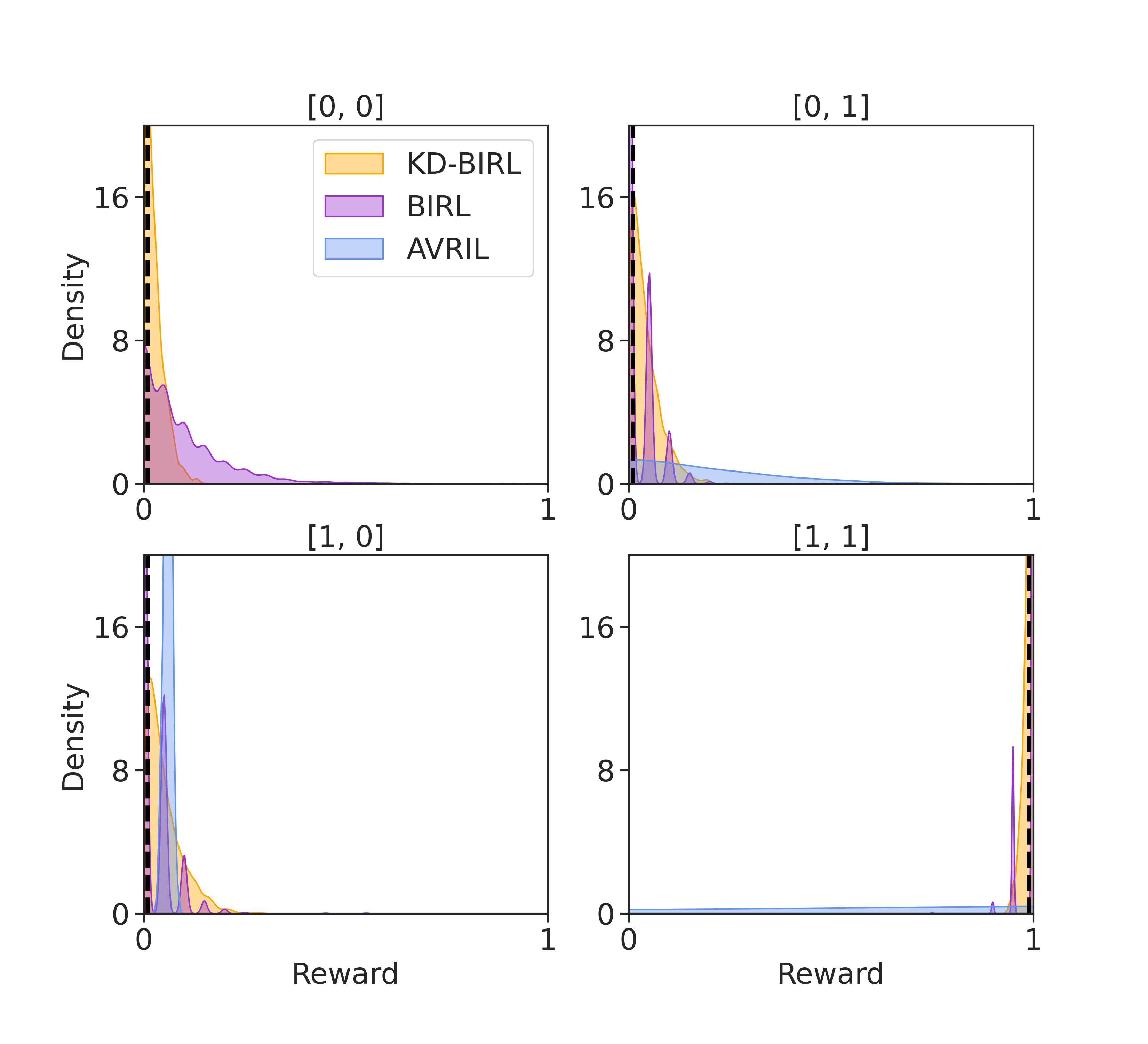
Figure 1: In a $2\times 2$ Gridworld, KD-BIRL’s posterior is comparable to BIRL, and is more concentrated towards $R^{\star}$ than AVRIL. Dashed vertical lines display the true reward in each state. The x-axis represents the numeric value of the sampled reward marginalized at the given state and the y-axis represents the density. A perfect marginalized posterior distribution would have the highest density at $R^{\star}$ in each state. AVRIL’s reward estimates are less concentrated than either KD-BIRL or BIRL.

KD-BIRL requires fewer instances of Q-learning than AVRIL or BIRL to produce accurate posterior samples. The setting is a $4\times 4$ Gridworld in which the state $[3,3]$ has a reward of 1 and all other states have zero reward. BIRL requires forward RL during every iteration of MCMC sampling; several thousand iterations are required for the sampler to converge. In contrast, AVRIL uses one instance of forward RL to learn an approximate posterior. KD-BIRL also minimizes the use of forward RL, only using it during dataset generation in this simulated setting.

We vary the number of iterations of forward RL and plot the EVDs. With fewer instances of forward RL, KD-BIRL learns a reward distribution superior to that of BIRL, partly because the the x-axis implies too few iterations of MCMC sampling; consequently, even though AVRIL requires fewer instances of forward RL, this comes at the expense of accuracy in the posterior distribution (Figure 2).

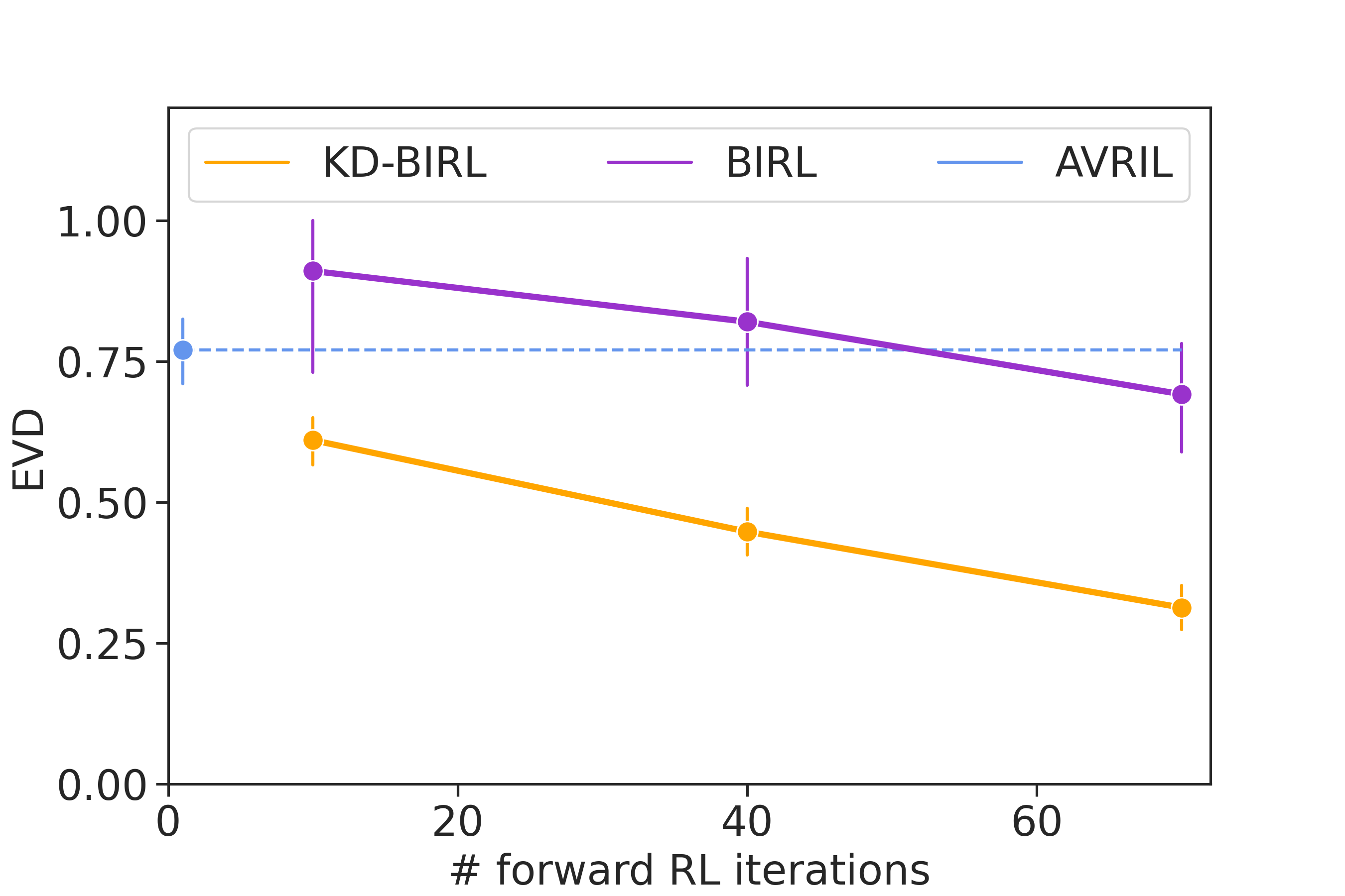
Figure 2: KD-BIRL requires fewer instances of RL to produce reward samples with lower EVD. We investigate a $4\times 4$ Gridworld environment where only the state $[3,3]$ receives positive reward. The x-axis represents the number of forward RL instances, the y-axis denotes EVD, and error bars correspond to standard error. The BIRL reward samples continue to have higher EVDs than those of KD-BIRL even with many instances of RL (each corresponding to an iteration of MCMC). AVRIL performs forward RL only once, but the EVD stagnates.

CKDE’s performance is limited in high state-space dimensions. It is well known that CKDE has difficulty scaling to high-dimensional probability density functions (Izbicki and Lee, 2017). Regardless, we identify the limits of the CKDE used in the original KD-BIRL setup, without a feature-based reward function, using a $5\times 5$ Gridworld environment. We find that KD-BIRL is able to estimate a posterior whose mean is in the equivalence class of $R^{\star}$; in other words, the expert demonstrations are equally likely under the posterior mean and $R^{\star}$ (Figure 3). However, there are states ($[2,3],[4,3]$ in Figure 3, Panel $2$) in the $5\times 5$ Gridworld in which the mean estimated reward is notably incorrect, which suggests that the CKDE struggles to learn 25 independent reward parameters successfully.

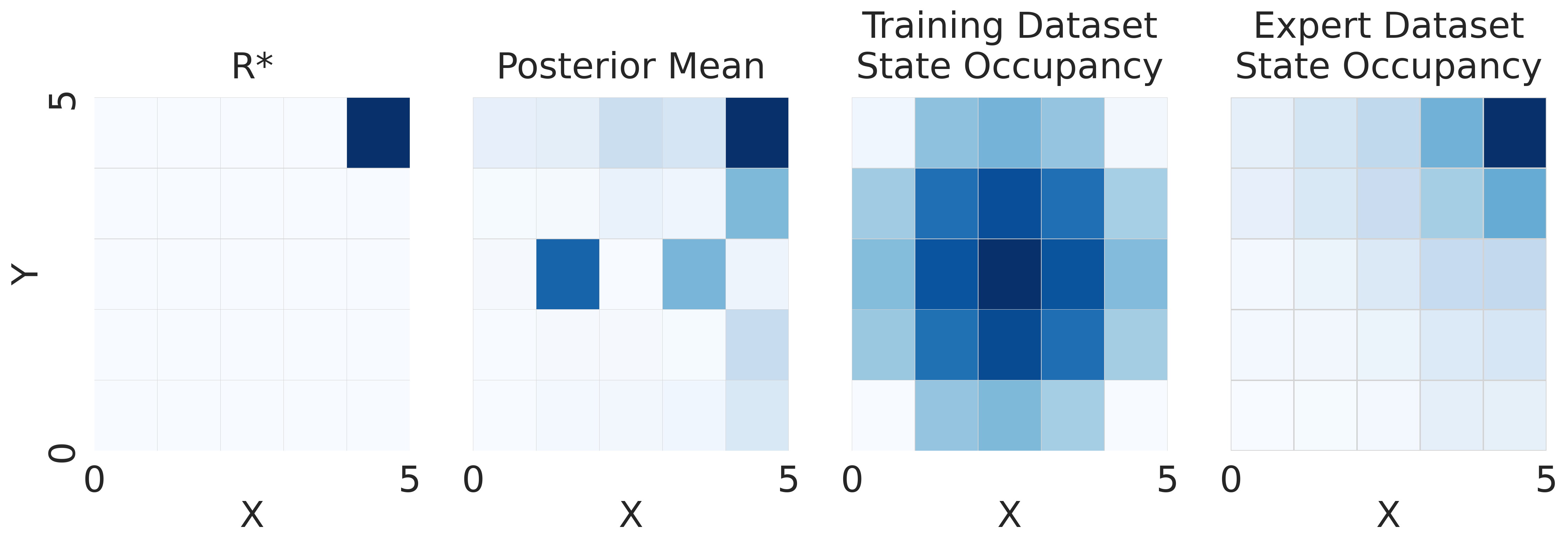
Figure 3: The CKDE is limited by the number of reward function parameters. We investigate a $5\times 5$ Gridworld environment in which the reward is positive in one state. The first panel shows $R^{\star}$, the second panel shows the KD-BIRL posterior mean, and the third and fourth panels show the training and expert demonstrations state occupancy. The KD-BIRL posterior mean is within the equivalence class of $R^{\star}$, because the darkest square is in the upper right hand corner, but there are incorrect estimates of reward in other states.

5.2 Feature-based reward function

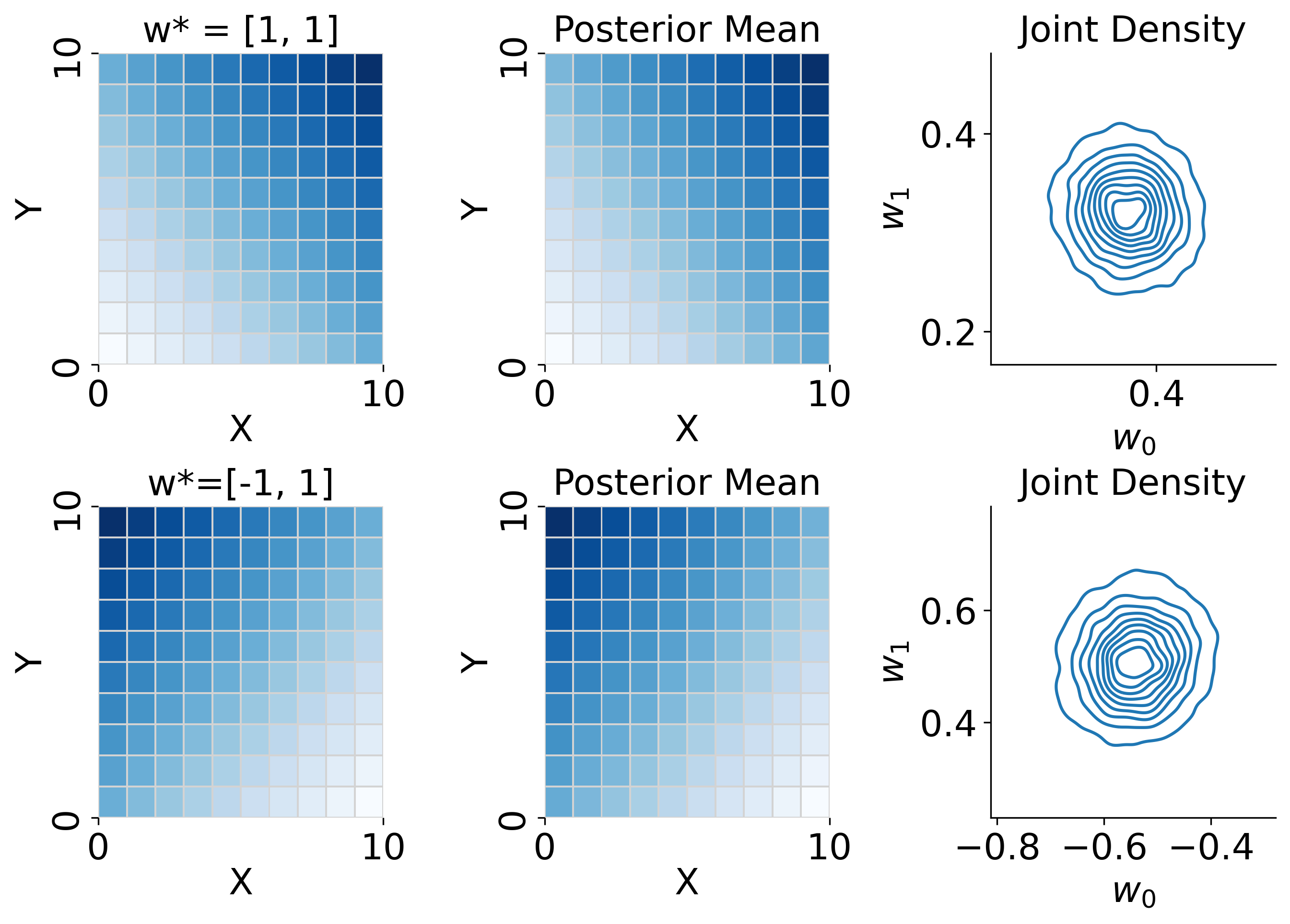
Figure 4: Using known features to parameterize reward enables reward inference in a 10x10 Gridworld. We learn the weights $w^{\star}=[1,1]$ (top) and $w^{\star}=[-1,1]$ (bottom). The first column visualizes $w^{\star}$ projected onto the Gridworld, the second visualizes the KD-BIRL posterior mean, and the third shows the joint density plots of the two weights, with the first on the x-axis and the second on the y-axis. KD-BIRL accurately infers the relative magnitude and sign of the individual weights.

To enable a CKDE-based likelihood to infer higher-dimensional reward functions, we use reward function featurization. We first investigate a $10\times 10$ Gridworld, and then study a Sepsis management task (Amirhossein Kiani, 2019), where the objective is to successfully discharge a patient (details in Appendix 12).

Selecting known features enables posterior inference in a $10\times 10$ Gridworld. In the $10\times 10$ Gridworld, the state space $\mathcal{S}$ is the series of one-hot encoded vectors of length $100$. In this setting, we select $\phi(s)=[x,y]$ to be a simple function that maps the state vector to the spatial coordinates of the agent. In this way, we treat the coordinates of the agent as a “feature vector.” Then, we choose weights $w^{\star}$ such that $R^{\star}$ is a linear combination of the features and $w^{\star}$. We visualize the resulting posterior distributions to demonstrate that KD-BIRL accurately recovers the relative magnitude and sign of the individual weights $w^{\star}$ for the two settings (Figure 4).

Using a variational autoencoder (VAE) to represent $\phi$ effectively summarizes state information in a Sepsis treatment environment. We use a VAE to learn a low-dimensional representation of state-action tuples, and aim to learn the set of weights to form the reward function. To do this, we learn $\phi$ on a set of state-action tuples independent of the training or expert demonstrations. The input dimension to the VAE is 47 (46 state features, 1 action), and the low dimensional representation has 3 features.

In four settings, each with a different $w^{\star}$, KD-BIRL’s posterior samples generate substantially lower EVD than AVRIL (Figure 5). In particular, KD-BIRL achieves lower EVD in the low-data regime where $n<1000$, indicating that it is able to learn an accurate posterior with few expert demonstrations. This, coupled with asymptotic posterior contraction guarantees, makes KD-BIRL a superior choice for performing IRL in with few expert demonstrations.

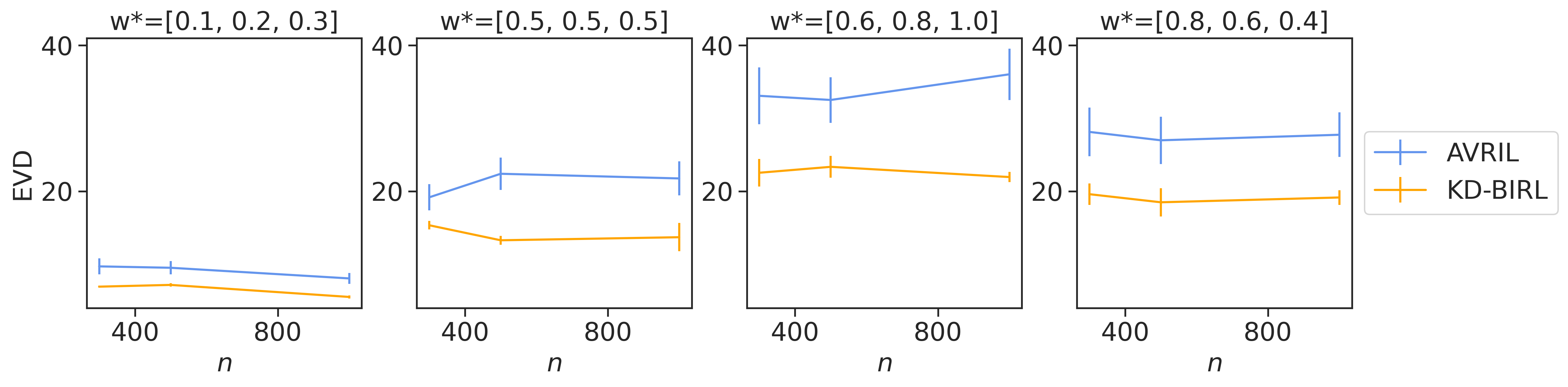
Figure 5: KD-BIRL achieves lower EVD in a Sepsis treatment environment than AVRIL, especially in a low-data regime. We evaluate 4 settings, each with a different $w^{\star}$. The x-axis corresponds to the number of expert demonstrations, $n$, the y-axis corresponds to EVD, and error bars indicate standard error. In a low-data regime ($n<1000$), KD-BIRL achieves much lower EVD than AVRIL, indicating greater posterior accuracy with fewer expert demonstrations.

6 Discussion

In this work, we present kernel density Bayesian inverse reinforcement learning (KD-BIRL), an IRL algorithm that improves upon existing methods by estimating a posterior distribution on the reward function while avoiding $Q$-learning for every iteration of MCMC sampling, thus reducing computational complexity and guaranteeing rational posterior updates. We also provide theoretical guarantees of posterior consistency. Our experiments demonstrate that KD-BIRL learns concentrated posteriors and is more computationally efficient than existing methods in a Gridworld environment. Additionally, we demonstrate that KD-BIRL can perform inference in a high dimensional sepsis treatment task by using a feature-based reward function; the resulting posterior outperforms a leading method especially in a low-data regime. Taken together, our results suggest that KD-BIRL can enable an accurate probabilistic description of objectives that is not possible with current methods.

Several future directions remain. The particular choices of distance metrics and hyperparameters used in the CKDE depend on the environment and reward function parameterization; additional experimentation is required to adapt this to different environments. Furthermore, KD-BIRL can be easily modified to accommodate other choices for the CKDE to improve performance in high dimensions. One approach could use a modified version of the CKDE to speed it up (Holmes et al., 2007). Another way to scale to higher dimensionality is to replace the CKDE with another nonparametric conditional density estimator (Rojas et al., 2005; Hinder et al., 2021). Finally, future applications will include additional settings with continuous state spaces, such as characterizing biophysical movement.

7 Possible irrationality of Q-based likelihoods

The original Bayesian IRL algorithm uses a $Q$-value function as a component of the likelihood calculation. There is a chance that the posterior updates resulting from using the likelihood function based on a $Q$-value function may not satisfy rationality considerations (P. G. Bissiri, 2016). Intuitively, rational updates imply that new evidence is appropriately incorporated to modify the posterior from the prior. The $Q$-value function can be approximated using any real-value prediction method from neural networks to linear regression, and the rationality of the resulting posterior updates is not discussed in prior work. A rational posterior update implies that if the updating function, in this case, $Q^{\star}$, has a lower value, the posterior probabilities should be lower, and vice versa. More specifically, a $Q$-value function must fulfill the following assumptions to ensure rational updates.

P. G. Bissiri (2016) assert that in order to guarantee rational updates to a posterior distribution, the following assumptions must be verified. We rephrase the assumptions in terms of notation that is familiar to readers of reinforcement learning literature. These are:

Assumption 1.

$$\psi[-Q_{\theta}(x_{2}),\psi\{-Q_{\theta}(x_{1}),p(\theta)\}]\equiv\psi\{-Q_{\theta}(x_{1})+-Q_{\theta}(x_{2}),p(\theta)\}$$

where $\theta$ is the parameter of interest, $p(\theta)$ is the prior distribution on $\theta$, $-Q_{\theta}$ is a loss function, here represented as a $Q$-value function parameterized by $\theta$, $\psi$ is the update function, and $x_{1},x_{2}$ are data points.

Assumption 2.

For any set $A\subset\Theta$,

$$\frac{\psi\{-Q_{\theta}(x),p(\theta)\}}{\int_{A}\psi\{-Q_{\theta}(x),p(\theta)\}d\theta}=\psi\{-Q_{\theta}(x),\mathrm{Pr}_{A}(\theta)\}$$

where $\mathrm{Pr}_{A}(\theta)$ is $p(\theta)$ normalized to $A$.

Assumption 3.

Lower evidence for a state should yield smaller posterior probabilities under the same prior. So, if for some $A\subset\Theta$, $-Q_{\theta}(x)>-Q_{\theta}(y)$ for $\theta\in A\subset\Theta$ and $-Q_{\theta}(x)=-Q_{\theta}(y)$ for $\theta\in A^{c}$, then

$$\int_{A}\psi\{-Q_{\theta}(x),p(\theta)\}d\theta<\int_{A}\psi\{-Q_{\theta}(y),p(\theta)\}d\theta.$$

Assumption 4.

If $-Q_{\theta}(x)\equiv$ constant, then $\psi\{l-Q_{\theta}(x),p(\theta)\}\equiv p(\theta)$.

Assumption 5.

If $-\widetilde{Q}_{\theta}(x)=-Q_{\theta}(x)+c$ for some constant $c$, then

$$\psi\{-\widetilde{Q}_{\theta}(x),p(\theta)\}=\psi\{-Q_{\theta}(x),p(\theta)\}.$$

These assumptions must be verified for a $Q$-value function if it is used to approximate the likelihood. It is possible to construct a rather simple $Q$-value function used for likelihood estimation that does not satisfy the criteria for posterior update rationality in P. G. Bissiri (2016). We construct a counterexample in which a likelihood that uses a $Q$-value function violates Assumption 3 for some set of input data. In the counterexample posed,the $Q$-value function is a simple piece-wise linear function. Let $\Theta=[-1,1]$, $A=[0,1]\subset\Theta$. define

$$-Q_{\theta}(x)\coloneqq\mathbbm{1}_{\{\theta\geq 0\}}x.$$

Now consider two demonstrations, or pieces of evidence: $x=1$, $y=0.5$. When we calculate $-Q_{\theta}$ for each of these demonstrations: $-Q_{\theta}(x)=\begin{cases}0&\theta\in[-1,0)\\ 1&\theta\in[0,1]\end{cases}$, $-Q_{\theta}(y)=\begin{cases}0&\theta\in[-1,0)\\ 0.5&\theta\in[0,1]\end{cases}$.

That is, $-Q_{\theta}(x)>-Q_{\theta}(y)$ when $\theta\in A$, while $-Q_{\theta}(x)=-Q_{\theta}(y)$ when $\theta\in A^{c}$. Define $p(\theta)=\frac{1}{2}$ to be the uniform prior.

Now we focus on the left-hand side (LHS) of the inequality in Assumption 3:

$$\mathrm{LHS} =\int_{0}^{1}\frac{p(\theta)e^{Q_{t}heta(x)}}{\int_{-1}^{1}p(\theta)e^{Q_{\theta}(x)}\mathrm{d}\theta}\mathrm{d}\theta$$

$$=\frac{\int_{0}^{1}e^{-1}\mathrm{d}\theta}{\int_{-1}^{0}1\mathrm{d}\theta+\int_{0}^{1}e^{-1}\mathrm{d}\theta}$$

$$=\frac{e^{-1}}{1+e^{-1}}\approx 0.3873.$$

Similarly, the right-hand side (RHS) is

$$\mathrm{RHS} =\int_{0}^{1}\frac{p(\theta)e^{Q_{\theta}(x)}}{\int_{-1}^{1}p(\theta)e^{Q_{\theta})(x)}\mathrm{d}\theta}\mathrm{d}\theta$$

$$=\frac{\int_{0}^{1}e^{-0.5}\mathrm{d}\theta}{\int_{-1}^{0}1\mathrm{d}\theta+\int_{0}^{1}e^{-0.5}\mathrm{d}\theta}$$

$$=\frac{e^{-0.5}}{1+e^{-0.5}}\approx 0.3775.$$

We show LHS $>$ RHS, which contradicts Assumption 3. In words, the “likelihood" or “evidence" of observing $x$ given $\theta\in A$ is smaller than the “likelihood" or “evidence" of observing $y$ given $\theta\in A$, so we expect the posterior distribution has less mass on A when observe $x$ (LHS) than $y$ (RHS), but the above inequality suggests otherwise. Hence, this update is not rational.

8 Proofs for Lemma 4.1 and Theorem 4.2

The proof associated with Lemma 4.1 follows.

Proof of Lemma 4.1.

We now use the continuity of the likelihood, the finite sample analysis of multivariate kernel density estimators in Wand and Jones (1994)[Section 4.4, Equation 4.16], which defines the Mean Integrated Square Error (MISE) of the density function, and Theorem 1 of Chacón and Duong (2018)[Section 2.6-2.9], which asserts that as the sample size increases, the mean of the density estimator converges and variance prevents the mean from exploding. We can use Theorem 1 because we assume that the density function is square-integrable and twice differentiable and that the bandwidth approaches 0 as the dataset size increases. Then, up to a constant, for a given state-action pair $(s,a)$,

$$\frac{1}{m}\sum_{j=1}^{m}e^{-d_{s}((s,a),(s_{j},a_{j}))^{2}/(2h)}e^{-d_{r}(R,R_{j})^{2}/(2h^{\prime})}\xrightarrow[m\to\infty]{P}p(s,a,R).$$

The same holds true for $d_{r}$, $\frac{1}{m}\sum_{\ell=1}^{m}e^{-d_{r}(R,R_{\ell})^{2}/(2h^{\prime})}\xrightarrow[m\to\infty]{P}p(R)$. By the Continuous Mapping Theorem (Mann and Wald, 1943), we conclude that

$$\widehat{p}_{m}(s,a|R)=\frac{\frac{1}{m}\sum_{j=1}^{m}e^{-d_{s}((s,a),(s_{j},a_{j}))^{2}/(2h)}e^{-d_{r}(R,R_{j})^{2}/(2h^{\prime})}}{\frac{1}{m}\sum_{\ell=1}^{m}e^{-d_{r}(R,R_{\ell})^{2}/(2h^{\prime})}}\xrightarrow[m\to\infty]{P}\frac{p(s,a,R)}{p(R)}=p(s,a|R).$$

∎

Now we prove Theorem 4.2.

Proof of Theorem 4.2.

By Lemma 4.1, as $m\to\infty$, $\widehat{p}_{m}$ converges to the true likelihood, so we can adopt existing tools from Bayesian asymptotic theory.

We first define an equivalence relation on $\mathcal{R}$, denoted by $\simeq$:

$$R_{1}\simeq R_{2}\leavevmode\nobreak\ \text{iff}\leavevmode\nobreak\ p(\cdot|R_{1})=p(\cdot|R_{2}),\leavevmode\nobreak\ a.e.$$

Note that $\simeq$ satisfies reflexivity, symmetry, and transitivity and is, therefore an equivalence relation. We denote the equivalence class by $[\cdot]$, that is, $[R]=\{R^{\prime}:R^{\prime}\simeq R\}$, and the quotient space is defined as $\widetilde{\mathcal{R}}\coloneqq\mathcal{R}/\mathord{\simeq}=\{[R]:R\in\mathcal{R}\}$. The corresponding canonical projection is denoted by $\uppi:\mathcal{R}\to\widetilde{\mathcal{R}},\leavevmode\nobreak\ R\mapsto[R]$. Then, the projection $\uppi$ induces a prior distribution on $\widetilde{\mathcal{R}}$ denoted by $\widetilde{\mathcal{P}}$: $\widetilde{\mathcal{P}}(A)\coloneqq\mathcal{P}(\uppi^{-1}(A))$. Moreover, $\widetilde{\mathcal{R}}$ admits a metric $\widetilde{d}$:

$$\widetilde{d}([R_{1}],[R_{2}])\coloneqq\|p(\cdot|R_{1})-p(\cdot|R_{2})\|_{L^{1}}.$$

Because this metric uses the $L^{1}$ norm, it satisfies symmetry and triangular inequality. Additionally, it is true that

$$\widetilde{d}([R_{1}],[R_{2}])=0\Longleftrightarrow p(\cdot|R_{1})=p(\cdot|R_{2}),\leavevmode\nobreak\ a.e.\Longleftrightarrow R_{1}\simeq R_{2}\Longleftrightarrow[R_{1}]=[R_{2}],$$

so $\widetilde{d}$ fulfills the Identity of Indiscernibles principle. As a result, $\widetilde{d}$ is a valid distance metric on $\widetilde{\mathcal{R}}$.

Then consider the following Bayesian model:

$$(s,a)|[R]\simeq p(s,a|[R]),\leavevmode\nobreak\ [R]\in\widetilde{\mathcal{R}},\leavevmode\nobreak\ [R]\simeq\widetilde{\mathcal{P}}.$$

This model is well-defined since $p(s,a|[R])$ is independent of the representative of $[R]$ by the definition of the equivalence class. Observe that $\mathrm{KL}(R,R^{*})=\mathrm{KL}([R],[R^{*}])$ by the definition of the equivalence class. Then, let $A=\{[R]:\mathrm{KL}([R],[R^{*}])<\epsilon\}\subset\widetilde{\mathcal{R}}$. We can define $\uppi^{-1}(A)=\{R\in\mathcal{R}:\mathrm{KL}(R,R^{*})<\epsilon\}\subset\mathcal{R}$. As a result, $\widetilde{\mathcal{P}}(\{[R]:\mathrm{KL}([R],[R^{*}])<\epsilon\})=\mathcal{P}(\{R:\mathrm{KL}(R,R^{*})<\epsilon\})>0$ for any $\epsilon>0$, that is, the KL support condition is satisfied . Moreover, the mapping $[R]\to p(\cdot|R)$ is one-to-one. Because the Bayesian model is parameterized by $[R]$ and we assume that $\mathcal{R}$ is a compact set, by  van der Vaart (2000)[Lemma 10.6] there exist consistent tests as required in Schwartz’s Theorem  (Ghosal and van der Vaart, 2017)[Example 6.19] . Then, by Schwartz (1965), the posterior $\widetilde{\mathcal{P}}^{n}_{m}$ on $\widetilde{\mathcal{R}}$ is consistent. That is, for any $\epsilon>0$, $\widetilde{\mathcal{P}}^{n}_{m}(\{[R]:\widetilde{d}([R],[R^{*}])<\epsilon\})\xrightarrow[n\to\infty]{m\to\infty}1$. Put in terms of the original parameter space,

$$\mathcal{P}_{m}^{n}(\{R:\|p(\cdot|R)-p(\cdot|R^{\star})\|_{L_{1}}<\epsilon)\})=\widetilde{\mathcal{P}}^{n}_{m}(\{[R]:\widetilde{d}([R],[R^{*}])<\epsilon\})\xrightarrow[n\to\infty]{m\to\infty},\leavevmode\nobreak\ \forall\epsilon>0.$$

∎

9 Code and experiments

Our experiments were run on an internally-hosted cluster using a 320 NVIDIA P100 GPU whose processor core has 16 GB of memory hosted. Our experiments used a total of approximately 200 hours of compute time. Our code uses the MIT License.

To fit KD-BIRL we use Stan (Team, 2011), which uses a Hamiltonian Monte Carlo algorithm. To fit the BIRL and AVRIL posteriors, we first generate the same number of expert demonstration trajectories as used for KD-BIRL. BIRL and AVRIL use an inverse temperature hyperparameter, $\alpha$; we set $\alpha=1$ for all methods. AVRIL uses two additional hyperparameters $\gamma,\delta$, which we set to 1. Unless otherwise specified, KD-BIRL uses a uniform prior for the reward $r_{s}\sim\text{Unif}(0,1)$ for $s=1,\dots,g\times g$ and Euclidean distance for $d_{s},d_{r}$.

For the $2\times 2$ and $4\times 4$ Gridworld environments, we specify the domain of each of these parameters to be the unit interval. For the $10\times 10$ Gridworld, the domain of $w$ is $[-1,1]$, and we use a Normal prior with mean $0$ and variance $1$ for $w^{\star}=[-1,1]$, and a Normal prior with mean $0.5$ and variance $0.5$ for $w^{\star}=[1,1]$.

For the Sepsis management task, we train a VAE to learn a low-dimensional state-representation $\phi$. The VAE uses 4 linear layers for the encoder and decoder, and optimizes for a downsampled representation with low reconstruction error using Adam. Because this is a simulated setting, once $\phi$ is known, it can be used to generate the required datasets. To do this, we first select a set of weights $w^{\star}$ for the expert demonstrations, and learn an optimal policy for $R(s,a)$ where $R(s,a)=\phi(s,a)\times w^{\star}$. Then, we generate state-action tuples (rollouts) from this policy. We repeat this procedure for several sets of uniformly selected weights $w_{0},\cdots,w_{c}$ to generate the training dataset.

10 KD-BIRL algorithm with dataset generation

We include a general version of the KD-BIRL algorithm in which the expert demonstrations and training dataset demonstrations are already available in the main text. A version of the algorithm that is suited for simulated datasets which require dataset generation can be seen in Algorithm 2.

Algorithm 2 Kernel Density Bayesian IRL in a simulated Environment

1:Input: MDP $M$, $k$, $m$, $n$, true reward $R^{\star}$, # MCMC iterations $c$

2:Generate $k$ reward functions $R_{1}\ldots,R_{k}\sim u$.

3:for $q=1,\dots,k$ do $\triangleright$ Generate training data

4:     $\pi_{q}:=\mathrm{PolicyIteration}(M,R_{q})$

5:     Generate $\lfloor m/k\rfloor$ demonstrations using agent $\pi_{q}$

6:end for

7:$\pi_{opt}:=\mathrm{PolicyIteration}(M,R^{\star})$

8:Generate $n$ demonstrations using agent $\pi_{opt}$ $\triangleright$ Generate expert data

9:for $l=1,\dots,c$ do

10:     Sample a reward function $\tilde{R}_{l}$ from the posterior distribution (Equation 6, main paper)

11:     Update the density function of the posterior $\widehat{p}_{m}^{n}$ using Equation 5 (main paper)

12:end for

13:Output: all sampled reward functions $\{R_{l}\}_{i=1}^{c}$

11 Gridworld Environment

The MDP here is defined by the grid’s $g\times g$ discrete state space $\mathcal{S}$ where a given state is represented as a one-hot encoded vector in $\mathcal{R}^{g\times g}$, $e_{i}$, where the $i$’th index is 1 and corresponds to the state in which the agent is in, and $g$ is the size of the grid; the action space contains 5 possible actions $\{\texttt{NO ACTION},\texttt{UP},\texttt{RIGHT},\texttt{LEFT},\texttt{DOWN}\}$, each represented as a one-hot encoded vector; and the true reward function $R^{\star}$, which is unobserved by the IRL algorithms, is a vector of length $g\times g$.

12 Sepsis Environment

The Sepsis environment is a simulation setting that models Sepsis treatment. There are $48$ state features (Table 1) in the original environment, comprised of $46$ physiological covariates and an action and state index.

Table 1: Features used in Sepsis environment

Feature	Description
Albumin	Measured value of Albumin, a protein made by the liver
Anion Gap	Measured difference between the negatively and positively charged electrolytes in blood
Bands	Measuring band neutrophil concentration
Bicarbonate	Measured arterial blood gas
Bilirubin	Measured bilirubin
BUN	Measured Blood Urea Nitrogen
Chloride	Measured chloride
Creatinine	Measured Creatinine
DiasBP	Diastolic blood pressure
Glucose	Administered glucose
Glucose	Measured glucose
Heart Rate	Measured Heart Rate
Hematocrit	Measure of the proportion of red blood cells
Hemoglobin	Measured hemoglobin
INR	International normalized ratio
Lactate	Measured lactate
MeanBP	Mean Blood Pressure
PaCO2	Partial pressure of Carbon Dioxide
Platelet	Measured platelet count
Potassium	Measured potassium
PT	Prothrombin time
PTT	Partial thromboplastin time
RespRate	Respiratory rate
Sodium	Measured sodium
SpO2	Measured oxygen saturation
SysBP	Measured systolic blood pressure
TempC	Temperature in degrees Celsius
WBC	White blood cell count
age	Age in years
is male	Gender, true or false
race	Ethnicity (white, black, hispanic or other)
height	Height in inches
Weight	Weight in kgs
Vent	Patient is on ventilator, true or false
SOFA	Sepsis related organ failure score
LODS	Logistic organ disfunction score
SIRS	Systemic inflammatory response syndrome
qSOFA	Quick SOFA score
qSOFA Sysbp Score	Quick SOFA that incorporates systolic blood pressure measurement
qSOFA GCS Score	Quick SOFA incorporating Glasgow Coma Scale
qSofa Respirate Score	Quick SOFA incorporating respiratory rate
Elixhauser hospital	Hospital uses Elixhauser comorbidity software
Blood culture positive	Bacteria is present in the blood

13 Calculating expected value difference (EVD)

The procedure to calculate EVD varies depending on the method. For all methods, this process requires a set of reward samples. Because KD-BIRL and BIRL both use MCMC sampling, we can use the reward samples generated from each iteration of MCMC. AVRIL does not use MCMC, so we have to modify the approach to generating samples depending on the structure of the reward function. When the reward function is a vector with length equal to the cardinality of the state space, we use the AVRIL agent to estimate the variational mean and standard deviation of reward at each state in the environment. Using these statistics, we then assume that the reward samples arise from a multivariate normal distribution and generate samples according to the mean and standard deviation. Once we have samples, we can then calculate EVD and 95% confidence intervals. Recall that EVD is defined as $|V^{\star}(r^{A})-V^{\pi(r^{L})}(r^{A})|$ where $r^{A}$ is the ground truth known reward and $r^{L}$ is the learned reward. For a given method, we calculate standard error across all sample rewards. Given a reward sample, we can calculate EVD, where $r^{L}$ is the sample, and $r^{A}$ is the known reward. To determine the value of the policy optimizing for a particular reward function, we train an optimal agent for that reward function, and generate demonstrations characterizing its behavior; the value is then the average reward received across those demonstrations. Finally, we calculate the difference between the value of the policy for $r^{A}$ and $r^{L}$, and report confidence intervals across these values for all samples for a given method.

In the Sepsis environment, because the state space is not discrete, we cannot use the above approach. To generate EVDs, we used the trained AVRIL agent to generate trajectories using agent-recommended actions starting from an initial state; the EVD here is the difference between the value of these trajectories and the value of trajectories generated using $w^{\star}$ (independent of AVRIL).

Bibliography

- Abbeel and Ng (2004) Pieter Abbeel and Andrew Y. Ng. Apprenticeship learning via inverse reinforcement learning. In The Twenty-First International Conference on Machine Learning, 2004.
- Adams et al. (2022) Stephen Adams, Tyler Cody, and Peter A. Beling. A survey of inverse reinforcement learning. Artificial Intelligence Review, Feb 2022. ISSN 1573-7462.
- Amirhossein Kiani (2019) Peter Henderson Amirhossein Kiani, Tianli Ding. Gymic: An OpenAI gym environment for simulating sepsis treatment for icu patients, 2019.
- Ashwood et al. (2020) Zoe Ashwood, Nicholas A. Roy, Ji Hyun Bak, and Jonathan W Pillow. Inferring learning rules from animal decision-making. In H. Larochelle, M. Ranzato, R. Hadsell, M.F. Balcan, and H. Lin, editors, Advances in Neural Information Processing Systems, volume 33, pages 3442–3453. Curran Associates, Inc., 2020.
- Balakrishnan et al. (2020) Sreejith Balakrishnan, Quoc Phong Nguyen, Bryan Kian Hsiang Low, and Harold Soh. Efficient exploration of reward functions in inverse reinforcement learning via Bayesian optimization. arXiv preprint arXiv:2011.08541, 2020.
- Brockman et al. (2016) Greg Brockman, Vicki Cheung, Ludwig Pettersson, Jonas Schneider, John Schulman, Jie Tang, and Wojciech Zaremba. OpenAI gym. arXiv preprint arXiv:1606.01540, 2016.
- Brown and Niekum (2018) Daniel S. Brown and Scott Niekum. Efficient probabilistic performance bounds for inverse reinforcement learning. In AAAI, 2018.
- Brown et al. (2020) Daniel S. Brown, Russell Coleman, Ravi Srinivasan, and Scott Niekum. Safe imitation learning via fast Bayesian reward inference from preferences, 2020.
- Cawley and Talbot (2010) Gavin C. Cawley and Nicola L. C. Talbot. On over-fitting in model selection and subsequent selection bias in performance evaluation. Journal of Machine Learning Research, 11(70):2079–2107, 2010.
- Chacón and Duong (2018) José E Chacón and Tarn Duong. Multivariate kernel smoothing and its applications. Chapman and Hall/CRC, 2018.
- Chan and van der Schaar (2021) Alex James Chan and Mihaela van der Schaar. Scalable Bayesian inverse reinforcement learning. In International Conference on Learning Representations, 2021.
- Choi and Kim (2012) Jaedeug Choi and Kee-eung Kim. Nonparametric Bayesian inverse reinforcement learning for multiple reward functions. In Advances in Neural Information Processing Systems, volume 25, 2012.
- Choi and Kim (2013) Jaedeug Choi and Kee-Eung Kim. Bayesian nonparametric feature construction for inverse reinforcement learning. In The Twenty-Third International Joint Conference on Artificial Intelligence, IJCAI ’13, 2013.
- Ghosal and van der Vaart (2017) Subhashis Ghosal and Aad van der Vaart. Fundamentals of nonparametric Bayesian inference, volume 44. Cambridge University Press, 2017.
- Hadfield-Menell et al. (2017) Dylan Hadfield-Menell, Smitha Milli, Pieter Abbeel, Stuart Russell, and Anca Dragan. Inverse reward design, 2017.
- Hinder et al. (2021) Fabian Hinder, Valerie Vaquet, Johannes Brinkrolf, and Barbara Hammer. Fast non-parametric conditional density estimation using moment trees. In 2021 IEEE Symposium Series on Computational Intelligence (SSCI), pages 1–7. IEEE, 2021.
- Holmes et al. (2007) Michael P. Holmes, Alexander G. Gray, and Charles Lee Isbell. Fast nonparametric conditional density estimation. In The Twenty-Third Conference on Uncertainty in Artificial Intelligence, UAI’07, Arlington, Virginia, USA, 2007. AUAI Press.
- Izbicki and Lee (2016) Rafael Izbicki and Ann B. Lee. Nonparametric conditional density estimation in a high-dimensional regression setting. Journal of Computational and Graphical Statistics, 25(4):1297–1316, 2016.
- Izbicki and Lee (2017) Rafael Izbicki and Ann B. Lee. Converting high-dimensional regression to high-dimensional conditional density estimation, 2017.
- Kolter et al. (2008) J Zico Kolter, Pieter Abbeel, and Andrew Y Ng. Hierarchical apprenticeship learning with application to quadruped locomotion. In Advances in Neural Information Processing Systems, pages 769–776. Citeseer, 2008.
- Levine et al. (2011) Sergey Levine, Zoran Popović, and Vladlen Koltun. Nonlinear inverse reinforcement learning with Gaussian processes. In The 24th International Conference on Neural Information Processing Systems, NIPS’11, page 19–27, Red Hook, NY, USA, 2011. Curran Associates Inc. ISBN 9781618395993.
- Mann and Wald (1943) Henry B Mann and Abraham Wald. On stochastic limit and order relationships. The Annals of Mathematical Statistics, 14(3):217–226, 1943.
- Michini and How (2012a) Bernard Michini and Jonathan P. How. Bayesian nonparametric inverse reinforcement learning. In Peter A. Flach, Tijl De Bie, and Nello Cristianini, editors, Machine Learning and Knowledge Discovery in Databases, pages 148–163, Berlin, Heidelberg, 2012a. Springer Berlin Heidelberg.
- Michini and How (2012b) Bernard Michini and Jonathan P. How. Improving the efficiency of Bayesian inverse reinforcement learning. In 2012 IEEE International Conference on Robotics and Automation, pages 3651–3656, May 2012b. doi: 10.1109/ICRA.2012.6225241.
- Michini et al. (2013) Bernard Michini, Mark Cutler, and Jonathan P. How. Scalable reward learning from demonstration. In 2013 IEEE International Conference on Robotics and Automation, pages 303–308, 2013. doi: 10.1109/ICRA.2013.6630592.
- Mombaur et al. (2010) Katja Mombaur, Anh Truong, and Jean-Paul Laumond. From human to humanoid locomotion—an inverse optimal control approach. Autonomous Robots, 28(3):369–383, 2010.
- Ng and Russell (2000) Andrew Y. Ng and Stuart Russell. Algorithms for inverse reinforcement learning. In in Proc. 17th International Conf. on Machine Learning, pages 663–670. Morgan Kaufmann Publishers Inc., 2000.
- P. G. Bissiri (2016) S. G. Walker P. G. Bissiri, C. C. Holmes. A general framework for updating belief distributions. Journal of the Royal Statistical Society. Series B (Statistical Methodology), 78(5), 2016.
- Qiao and Beling (2011) Qifeng Qiao and Peter A. Beling. Inverse reinforcement learning with Gaussian process. 2011 American Control Conference, pages 113–118, 2011.
- Ramachandran and Amir (2007) Deepak Ramachandran and Eyal Amir. Bayesian inverse reinforcement learning. In The 20th International Joint Conference on Artifical Intelligence, page 2586–2591, 2007.
- Ratliff et al. (2006a) Nathan Ratliff, David Bradley, J. Andrew Bagnell, and Joel Chestnutt. Boosting structured prediction for imitation learning. In Advances in Neural Information Processing Systems, page 1153–1160, 2006a.
- Ratliff et al. (2006b) Nathan D. Ratliff, J. Andrew Bagnell, and Martin A. Zinkevich. Maximum margin planning. In The 23rd International Conference on Machine Learning, ICML ’06, page 729–736, New York, NY, USA, 2006b. Association for Computing Machinery.
- Rojas et al. (2005) Alex L Rojas, Christopher R Genovese, Christopher J Miller, Robert Nichol, and Larry Wasserman. Conditional density estimation using finite mixture models with an application to astrophysics. Center for Automatic Learning and Discovery, Department of Statistics, Carnegie Mellon University, 2005.
- Rothkopf and Ballard (2013) Constantin A. Rothkopf and Dana H. Ballard. Modular inverse reinforcement learning for visuomotor behavior. Biol. Cybern., 107(4):477–490, aug 2013. ISSN 0340-1200.
- Schwartz (1965) Lorraine Schwartz. On Bayes procedures. Zeitschrift für Wahrscheinlichkeitstheorie und Verwandte Gebiete, 4:10–26, 1965.
- Silverman (1986) B. W. Silverman. Density Estimation for Statistics and Data Analysis. Chapman & Hall, London, 1986.
- Sutton and Barto (2018) Richard S. Sutton and Andrew G. Barto. Reinforcement Learning: An Introduction. A Bradford Book, Cambridge, MA, USA, 2018. ISBN 0262039249.
- Team (2011) Stan Development Team. Stan modeling language users guide and reference manual, version 2.29, 2011.
- van der Vaart (2000) Aad van der Vaart. Asymptotic Statistics, volume 3. Cambridge University Press, 2000.
- Verma et al. (2021) Archit Verma, Siddhartha G. Jena, Danielle R. Isakov, Kazuhiro Aoki, Jared E. Toettcher, and Barbara E. Engelhardt. A self-exciting point process to study multicellular spatial signaling patterns. Proceedings of the National Academy of Sciences, 118(32), 2021.
- Šošić et al. (2018) Adrian Šošić, Abdelhak M. Zoubir, Elmar Rueckert, Jan Peters, and Heinz Koeppl. Inverse reinforcement learning via nonparametric spatio-temporal subgoal modeling. J. Mach. Learn. Res., 19(1):2777–2821, jan 2018. ISSN 1532-4435.
- Wand and Jones (1994) Matt P Wand and M Chris Jones. Kernel smoothing. CRC press, 1994.
- Zheng et al. (2014) Jiangchuan Zheng, Siyuan Liu, and Lionel M. Ni. Robust Bayesian inverse reinforcement learning with sparse behavior noise. In Association for the Advancement of Artificial Intelligence, AAAI’14, page 2198–2205. AAAI Press, 2014.
- Ziebart et al. (2008) Brian D Ziebart, Andrew L Maas, J Andrew Bagnell, Anind K Dey, et al. Maximum entropy inverse reinforcement learning. In Association for the Advancement of Artificial Intelligence (AAAI), volume 8, pages 1433–1438. Chicago, IL, USA, 2008.
- Ziebart et al. (2009) Brian D. Ziebart, Andrew L. Maas, J. Andrew Bagnell, and Anind K. Dey. Human behavior modeling with maximum entropy inverse optimal control. In AAAI Spring Symposium: Human Behavior Modeling, 2009.