Transmission Efficiency Limit of Single-Switch Reconfigurable Transmitarray Elements

Abstract

Reconfigurable transmitarray antennas (RTAs) are rapidly gaining popularity, but optimizating their performance requires systematic design theories. In particular, a performance limit theory for RTA elements would be highly valuable. This paper presents a theory on the transmission efficiency limit of single-switch RTA elements. Using microwave network theory, we conduct an analytical investigation of single-switch RTA elements, revealing that the transmission coefficients under two states should be restricted within a specific unit circle on the Smith chart. The results are validated through analytical proof and numerical simulations. Additionally, this theory suggests that the transmission phase difference is tightly constrained by the transmission amplitudes, indicating that the phase-shifting ability of a single-switch RTA element is limited. These findings have significant implications for the design and optimization of RTAs.

I Introduction

Recent years have witnessed the rapid development of microwave metasurfaces, leading to the emergence of diverse high-gain array antennas with novel architectures, including reflectarray antennas (RAs), transmitarray antennas (TAs), and their reconfigurable versions [1, 2, 3, 4]. Along with the emergence of various prototypes, underlying theories have also been proposed to guide the design of these array antennas. Performance limit theories are particularly useful in predicting the performance of general structures before their actual design, which can significantly improve the design efficiency. Here are some examples of performance limit theories for these novel array antennas.

In 2014, the transmission phase limit theory for multilayer TA designs was first introduced in [5]. Figure 1(a) depicts a schematic illustration of the multilayer TA. Using microwave network models and S-parameters, researchers discovered the constraints on the transmission amplitude and phase of TA elements, demonstrating that the phase tuning range within a 1-dB transmission amplitude loss is 54^∘, 170^∘, 308^∘, and 360^∘ for single-, double-, triple-, and quad-layers.

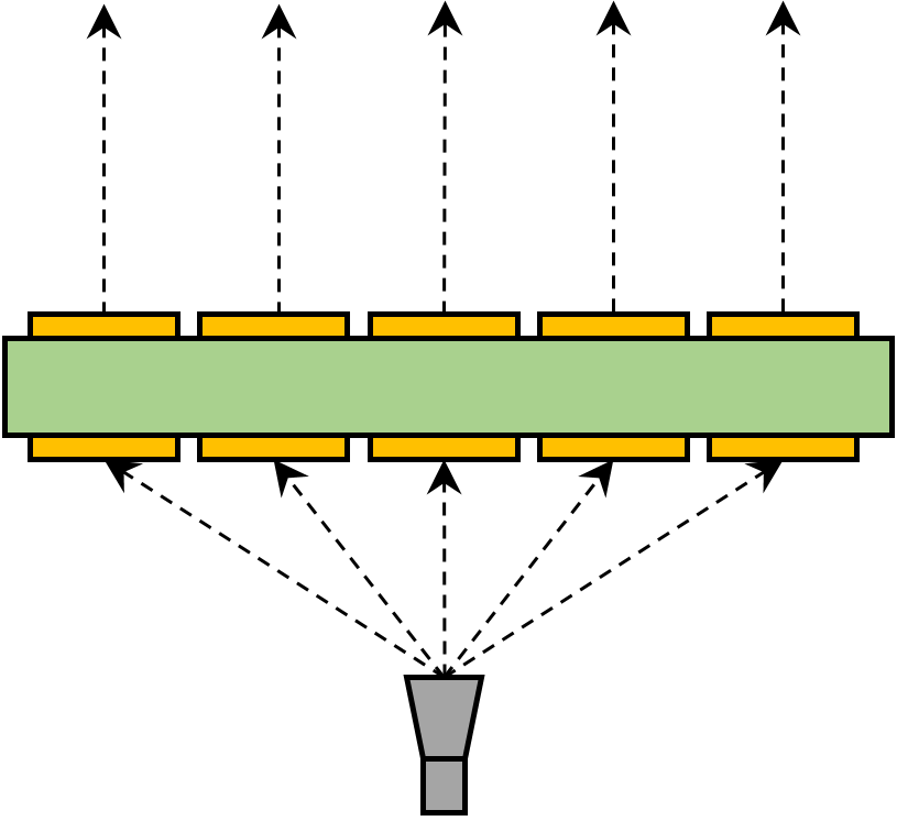
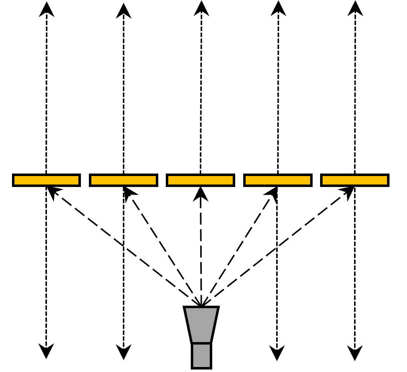
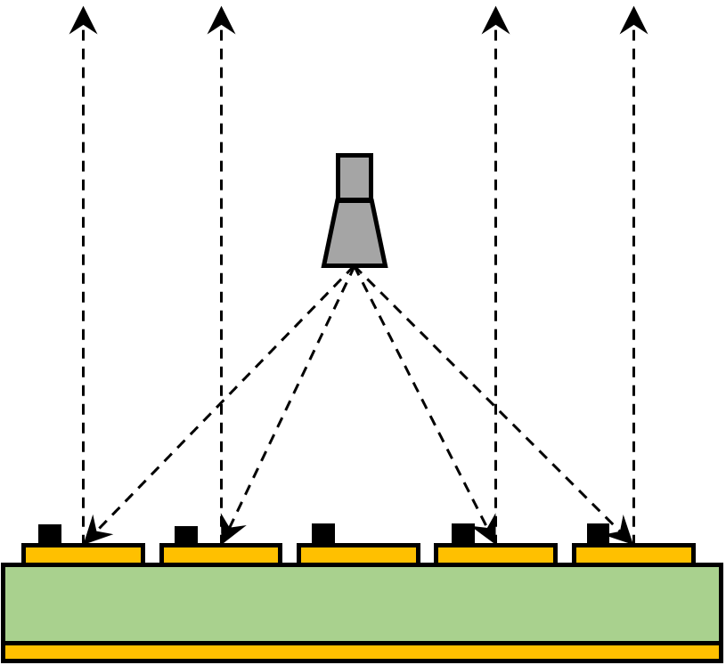
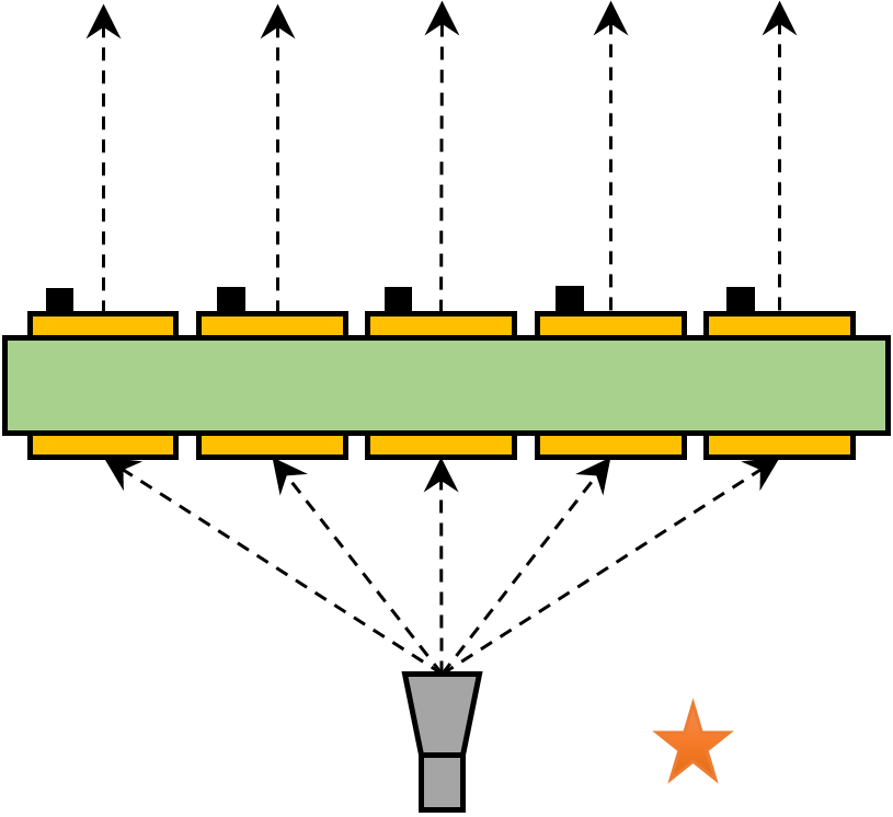
Figure 1: A schematic illustration of several novel array antennas. (a) Multilayer TA. (b) Near-zero-thickness transmit-reflect-array antenna. (c) Single-switch RRA. (d) Single-switch RTA.

Another instance of the performance limit theory pertains to transmit-reflect-array antennas based on polarization conversion methods, as revealed in 2018 [6]. A schematic of the this type of array antenna is shown in Fig. 1(b). By applying the electric field continuity condition on the near-zero-thickness surface, researchers found that to achieve 360^∘ phase coverage on both sides, a minimum of 6 dB amplitude loss is required.

Reconfigurable reflectarray antennas (RRAs) have emerged as a promising candidate for achieving beam-scanning capability. In particular, the 1-bit phase quantization technique has become a mainstream architecture in many applications, due to its minimal switch requirement with only 3 dB gain loss [7]. In recent years, several single-switch 1-bit RRAs with different features have been presented in [8, 13, 14, 15, 10, 18, 16, 11, 12, 17, 9, 19], as depicted in Fig. 1(c). Recently, a performance limit theory for single-switch RRA elements was presented based on the radiation viewpoint [20]. By pre-calculating the performance limit and design targets at given switch parameters, this theory can facilitate the efficient design of wideband, multiband, or high-frequency RRA elements.

Reconfigurable transmitarray antennas (RTAs) have been proposed as an alternative to RRAs to eliminate the feed blockage effect. Since 2012, 1-bit RTAs have been extensively studied, and various prototypes based on different principles have been proposed. For example, current reversal method utilizes at least two opposite switches on one layer to achieve accurate 180^∘ phase difference [21, 22, 23, 24, 25, 26, 27, 28, 29]. Recently, stacked-layer RTAs with two switches on different layers have been presented based on the resonant method, which can also achieve 1-bit phase difference at certain frequency bands [30, 31, 32].

Interestingly, it has been found that all of the aforementioned 1-bit RTA elements require at least two switches to achieve 1-bit phase difference with high transmission amplitude. This raises a question: Is it feasible to design a high-performance RTA element using only one switch? Fig. 1(d) provides an illustration of a single-switch RTA. Recently, by using three-port microwave network analysis, it is proven by contradiction that it is impossible to design a single-switch RTA element with both high transmission amplitude and 1-bit phase tuning ability simultaneously [33]. Therefore, the 1-bit RTA elements indeed require at least two switches theoretically. However, this proof only applies to the zero-reflection case, and it does not consider the general situation where the reflection coefficients are not necessarily zero. Therefore, a quantitative analysis of the performance of the single-switch RTA element in general cases needs to be further investigated.

To provide a quantitative performance limit in general situations, this paper presents a theory on the transmission efficiency limit for single-switch RTA elements. Geometrically, this theory states that the transmission coefficients under two states must vary on or inside a specific unit circle with a diameter of 1 on the Smith chart. An intuitive illustration of this conclusion is shown in Fig. 2. Based on this finding, it is concluded that the transmission phase difference is tightly constrained by the transmission amplitudes. Specifically, high transmission amplitudes result in a narrow transmission phase difference, while a phase difference of near 180^∘ results in low transmission amplitudes. This conclusion is consistent with the previous finding in [33].

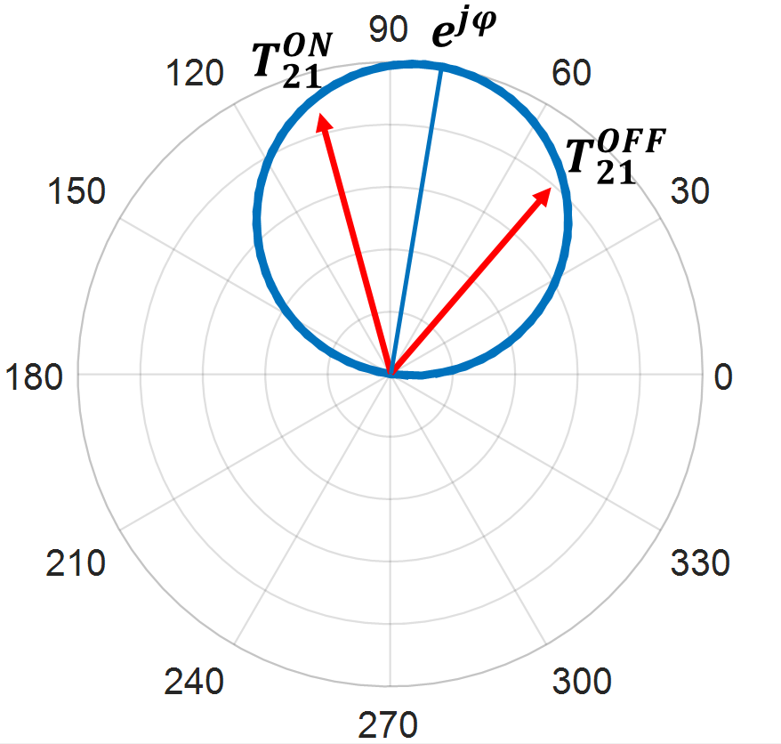
Figure 2: A geometric illustration of the transmission efficiency limit, where the two transmission coefficients should be contained within a certain circle on the Smith chart.

This paper is organized as follows. Section II introduces the microwave network model of the single-switch RTA elements and presents an important lemma. Section III presents the transmission efficiency limit theory and its proof of the single-switch RTA elements. The simulation verification of this limit theory is demonstrated in Section IV. Section V draws the conclusion.

II Model of Single-Switch RTA Elements

II-A The Microwave Network Model of the RTA Element with a Single Switch

The RTA element with a single switch can be modeled as a three-port microwave network [33], as shown in Fig. 3. The incoming wave enters the element through the Floquet port 1, and transmits toward the Floquet port 2. Since the size of the switch is much smaller than the wavelength, the lumped switch port 3 can be designated between the switch and the element. The passive structure is characterized by a 3$\times$3 scattering matrix $[S]$. According to the S-parameter definition [34], the incoming wave $[a]$ and outgoing wave $[b]$ are related through the $[S]$ matrix using the following formula

$$\left[\begin{array}[]{l}b_{1}\\ b_{2}\\ b_{3}\end{array}\right]=\left[\begin{array}[]{lll}S_{11}&S_{12}&S_{13}\\ S_{21}&S_{22}&S_{23}\\ S_{31}&S_{32}&S_{33}\end{array}\right]\cdot\left[\begin{array}[]{l}a_{1}\\ a_{2}\\ a_{3}\end{array}\right].$$ (1)

Here, $S_{ij}=S_{ji}$ due to reciprocity.

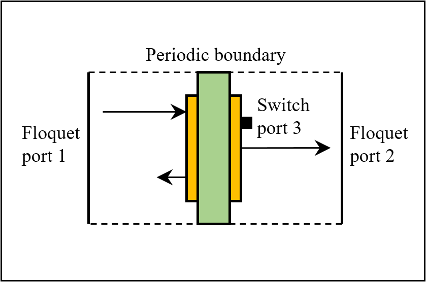
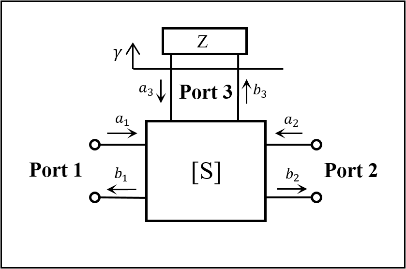
Figure 3: The model of an RTA element with a single switch. (a) A conceptual illustration of an RTA element. (b) The equivalent network model of the RTA element.

$\gamma$ is the reflection coefficient of the switch, which is defined as

$$\gamma=\frac{Z-\eta}{Z+\eta}=\frac{a_{3}}{b_{3}},$$ (2)

where $Z$ is the impedance of the switch, and $\eta$ is a reference characteristic impedance, typically 377 $\Omega$. Notably, the switch has two states, and thus, $\gamma$ takes on two distinct values: $\gamma_{\text{ON}}$ and $\gamma_{\text{OFF}}$.

II-B Lemma: Relation Among Reflection and Transmission Coefficients

As derived in [33], the reflection coefficient of port 1 ($\Gamma_{1}$) and the transmission coefficient from port 1 to port 2 ($T_{21}$) are expressed as follows

$$\Gamma_{1}=\frac{b_{1}}{a_{1}}=S_{11}+\frac{S_{13}^{2}\gamma}{1-S_{33}\gamma},$$ (3)

$$T_{21}=\frac{b_{2}}{a_{1}}=S_{21}+\frac{S_{23}S_{13}\gamma}{1-S_{33}\gamma}.$$ (4)

Similarly, the reflection coefficient of port 2 ($\Gamma_{2}$) is expressed as

$$\Gamma_{2}=\frac{b_{2}}{a_{2}}=S_{22}+\frac{S_{23}^{2}\gamma}{1-S_{33}\gamma}.$$ (5)

We denote the reflection coefficients under ON/OFF switch states as $(\Gamma^{\text{ON}}_{1},\Gamma^{\text{OFF}}_{1})$ and $(\Gamma^{\text{ON}}_{2},\Gamma^{\text{OFF}}_{2})$, and the transmission coefficients under ON/OFF switch states as $(T^{\text{ON}}_{21},T^{\text{OFF}}_{21})$. Then we define the difference of the coefficients between two states as follows

$$\Delta\Gamma_{1}=\Gamma^{\text{ON}}_{1}-\Gamma^{\text{OFF}}_{1}=\frac{S_{13}^{2}\gamma_{\text{ON}}}{1-S_{33}\gamma_{\text{ON}}}-\frac{S_{13}^{2}\gamma_{\text{OFF}}}{1-S_{33}\gamma_{\text{OFF}}},$$ (6)

$$\Delta\Gamma_{2}=\Gamma^{\text{ON}}_{2}-\Gamma^{\text{OFF}}_{2}=\frac{S_{23}^{2}\gamma_{\text{ON}}}{1-S_{33}\gamma_{\text{ON}}}-\frac{S_{23}^{2}\gamma_{\text{OFF}}}{1-S_{33}\gamma_{\text{OFF}}},$$ (7)

$$\Delta T_{21}=T^{\text{ON}}_{21}-T^{\text{OFF}}_{21}=\frac{S_{23}S_{13}\gamma_{\text{ON}}}{1-S_{33}\gamma_{\text{ON}}}-\frac{S_{23}S_{13}\gamma_{\text{OFF}}}{1-S_{33}\gamma_{\text{OFF}}}.$$ (8)

From (6), (7), and (8), it is evident that the following relation holds

$$\Delta T^{2}_{21}=\Delta\Gamma_{1}\Delta\Gamma_{2}.$$ (9)

This expression shows a clear relationship on differences of reflection and transmission coefficients in a single-switch RTA element, and reduces the three-port network to a two-port network analysis by incorporating the switch parameters into the reflection and transmission coefficients, as illustrated in Fig. 4. We define a reduced 2$\times$2 scattering matrix $[S^{\prime}]$ as follows

$$[S^{\prime}]=\left[\begin{array}[]{ll}\Gamma_{1}&T_{21}\\ T_{21}&\Gamma_{2}\end{array}\right],$$ (10)

which represents the scattering behavior of the entire element.

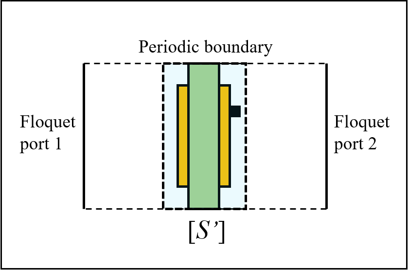
Figure 4: The two-port microwave network model of the entire single-switch RTA element.

III The Constraint on the Two Transmission Coefficients of Single-Switch RTA Elements

In this section, we utilize (9) and (10) to derive the transmission efficiency limit of a single-switch RTA element. The key result is stated first, and then proven under both symmetric and asymmetric conditions. We also derive the upper limit of the transmission phase difference as a corollary of the theory.

III-A The Transmission Efficiency Limit

The transmission efficiency limit of the single-switch RTA element is as follows: The two transmission coefficients under two switch states must lie on or within a unit circle with a diameter of 1. In other words, there exists a unit circle that can contain the two transmission coefficients for single-switch RTA element geometrically. An intuitive illustration of this finding has been shown in Fig. 2.

Mathematically, $T^{\text{ON}}_{21}$ and $T^{\text{OFF}}_{21}$ should satisfy the following condition

$$\exists\varphi\in[0,2\pi), \left|T^{\text{ON}}_{21}-\frac{e^{j\varphi}}{2}\right|\leq\frac{1}{2},$$ (11)

$$\left|T^{\text{OFF}}_{21}-\frac{e^{j\varphi}}{2}\right|\leq\frac{1}{2}.$$

The proof of this statement can be divided into two parts. First, for RTA elements with symmetric reflection coefficients, it can be theoretically proven that the two transmission coefficients must lie on the unit circle. Secondly, for RTA elements with asymmetric reflection coefficients, it can be analyzed and observed that the two transmission coefficients must lie within or on the unit circle.

III-B Proof for Symmetric RTA Elements

Assuming the single-switch RTA element is lossless, we can prove that the two transmission coefficients vary on the unit circle for symmetric elements.

The lossless condition implies that the scattering matrix $[S^{\prime}]$ is unitary, meaning that $[S^{\prime}][S^{\prime}]^{H}=I$, where $H$ denotes the Hermitian transpose. Using the results of our previous derivation in [20], we have

$$\left\{\begin{array}[]{l}\left|\Gamma_{1}\right|^{2}+\left|T_{21}\right|^{2}=1\\ \left|\Gamma_{2}\right|^{2}+\left|T_{21}\right|^{2}=1\\ \end{array}\right.$$ (12)

and

$$\frac{\theta_{1}+\theta_{2}}{2}-\theta_{21}=\pm\frac{\pi}{2},$$ (13)

where $\theta_{1}$ and $\theta_{2}$ are the reflection phases from two ports, respectively, and $\theta_{21}$ is the transmission phase.

Since the network is symmetric, the two reflection coefficients are equal, i.e.,

$$\Gamma_{1}=\Gamma_{2}.$$ (14)

This implies that $\theta_{1}=\theta_{2}$. Combining these results with (12) and (13), we obtain

$$\left\{\begin{array}[]{l}\left|\Gamma_{1}\right|^{2}+\left|T_{21}\right|^{2}=1\\ \theta_{1}-\theta_{21}=\pm\frac{\pi}{2}\\ \end{array}\right.$$ (15)

It can be mathematically shown that the complex numbers $\Gamma_{1}$ and $T_{21}$ have the following relations

$$T_{21}-\Gamma_{1}=e^{j\varphi},$$ (16)

or

$$T_{21}+\Gamma_{1}=e^{j\varphi},$$ (17)

where $\varphi$ is a parameter of this equation. A geometric illustration of these relations is shown on the Smith chart in Fig. 5. The vector $\Gamma_{1}$ and $T_{21}$ lie on the complex plane, and according to the Pythagorean theorem, they are perpendicular to each other, and the length of the hypotenuse is 1. Therefore, $T_{21}$, $e^{j\varphi}$ and $0$ form a circle on the Smith chart, and $e^{j\varphi}$ represents the diameter of the circle. In other words, for a given $e^{j\varphi}$, $T_{21}$ varies on the circle determined by $e^{j\varphi}$.

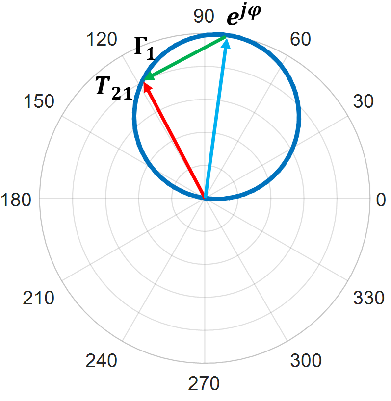
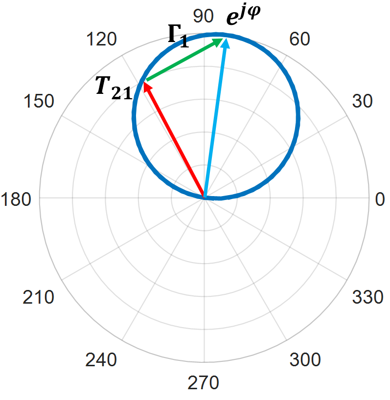
Figure 5: The geometric illustration of the relations between $T_{21}$ and $\Gamma_{1}$ on the Smith chart for the symmetric case. (a) An illustration of the relation in (16). (b) An illustration of the relation in (17).

Since $\Gamma_{1}=\Gamma_{2}$ in both states, the difference between them should also be equal, i.e., $\Delta\Gamma_{1}=\Delta\Gamma_{2}$. Substituting this relation into (9), the following expression is obtained

$$\Delta T^{2}_{21}=\Delta\Gamma^{2}_{1}.$$ (18)

There are two sets of solutions to this equation, which are discussed separately. Notably, it is assumed in advance that $T^{\text{ON}}_{21}$ varies on the circle determined by $e^{j\varphi^{\text{ON}}}$, and $T^{\text{OFF}}_{21}$ varies on the circle determined by $e^{j\varphi^{\text{OFF}}}$.

1. $\Delta T_{21}=\Delta\Gamma_{1}$. This equation leads to

   $$T^{\text{ON}}_{21}-\Gamma^{\text{ON}}_{1}=T^{\text{OFF}}_{21}-\Gamma^{\text{OFF}}_{1}.$$ (19)

   Based on (16) and (19), it is found that

   $$e^{j\varphi^{\text{ON}}}=e^{j\varphi^{\text{OFF}}},$$ (20)

   which means that $T^{\text{ON}}_{21}$ and $T^{\text{OFF}}_{21}$ vary on the same unit circle, as shown in Fig. 6(a).

2. $\Delta T_{21}=-\Delta\Gamma_{1}$. This equation leads to

   $$T^{\text{ON}}_{21}+\Gamma^{\text{ON}}_{1}=T^{\text{OFF}}_{21}+\Gamma^{\text{OFF}}_{1}.$$ (21)

   Based on (17) and (21), it is found that

   $$e^{j\varphi^{\text{ON}}}=e^{j\varphi^{\text{OFF}}},$$ (22)

   which means that $T^{\text{ON}}_{21}$ and $T^{\text{OFF}}_{21}$ vary on the same unit circle, as shown in Fig. 6(b).

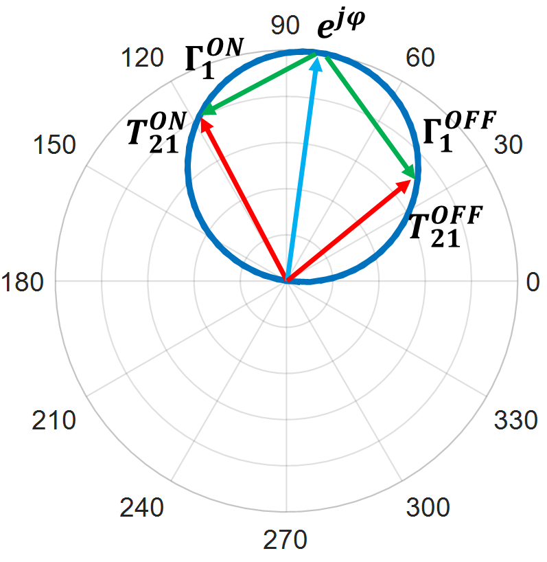
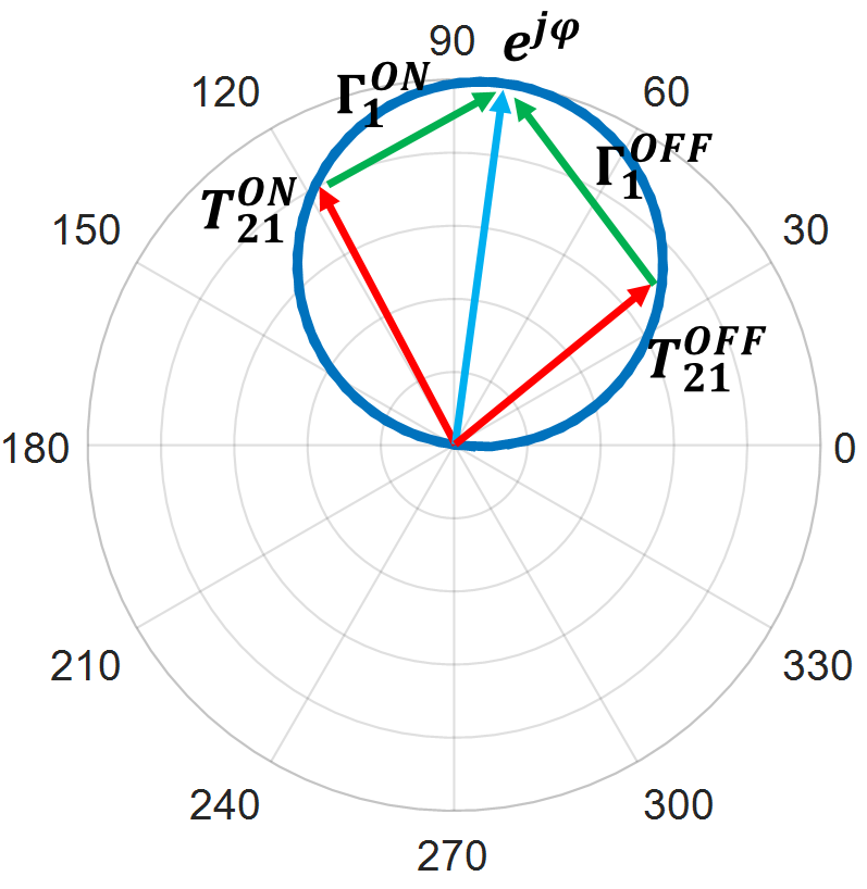
Figure 6: Illustration of the geometric method to solve (18). (a) $T^{\text{ON}}_{21}$ and $T^{\text{OFF}}_{21}$ vary on the same unit circle in case $\Delta T_{21}=\Delta\Gamma_{1}$. (b) $T^{\text{ON}}_{21}$ and $T^{\text{OFF}}_{21}$ vary on the same unit circle in case $\Delta T_{21}=-\Delta\Gamma_{1}$.

In summary, for lossless symmetric RTA elements, the two transmission coefficients should lie on the same unit circle.

III-C Analysis of Asymmetric RTA Elements

This part analyzes the asymmetric single-switch RTA elements, and it is observed that the two transmission coefficients should vary on or inside the unit circle.

Assume the element is lossless, so (12) and (13) still hold. From (12), it can be deduced that $\left|\Gamma_{1}\right|=\left|\Gamma_{2}\right|$. Because it is the relative relation between two transmission coefficients that matters, without loss of generality, one of the transmission coefficients, such as $T^{\text{ON}}_{21}$, can be assumed to vary on the unit circle determined by $e^{j0}=1$. An auxiliary variable $\Gamma^{\text{ON}}$ is introduced, with the equal amplitude to $\Gamma^{\text{ON}}_{1}$ and $\Gamma^{\text{ON}}_{2}$, and the phase is defined as $\theta^{\text{ON}}=(\theta^{\text{ON}}_{1}+\theta^{\text{ON}}_{2})/2$. Therefore, the relation between $\Gamma^{\text{ON}}$ and $T^{\text{ON}}_{21}$ can be expressed as

$$\left\{\begin{array}[]{l}\left|\Gamma^{\text{ON}}\right|^{2}+\left|T^{\text{ON}}_{21}\right|^{2}=1\\ \theta^{\text{ON}}-\theta^{\text{ON}}_{21}=\pm\frac{\pi}{2}\\ \end{array}\right.$$ (23)

Similar to the analysis in the symmetric case, $\Gamma^{\text{ON}}$ should be perpendicular to $T^{\text{ON}}_{21}$, and the length of the hypotenuse is 1. Fig. 7(a) shows a graphical representation of the relationship between reflection and transmission coefficients in (12) and (13). Additionally, as $\theta^{\text{ON}}=(\theta^{\text{ON}}_{1}+\theta^{\text{ON}}_{2})/2$, $\Gamma^{\text{ON}}$ lies on the angular bisector between $\Gamma^{\text{ON}}_{1}$ and $\Gamma^{\text{ON}}_{2}$. Let the phase difference between $\Gamma^{\text{ON}}$ and $\Gamma^{\text{ON}}_{1}$ be $\phi^{\text{ON}}$. Thus, the phase difference between $\Gamma^{\text{ON}}$ and $\Gamma^{\text{ON}}_{2}$ is $-\phi^{\text{ON}}$. Since the network is asymmetric, $\phi^{\text{ON}}$ is neither $0$ nor $\pi$. Based on the geometric insights, the reflection coefficients can be expressed as

$$\left\{\begin{array}[]{l}\Gamma^{\text{ON}}_{1}=(T^{\text{ON}}_{21}-1)e^{-j\phi^{\text{ON}}}\\ \Gamma^{\text{ON}}_{2}=(T^{\text{ON}}_{21}-1)e^{j\phi^{\text{ON}}}\\ \end{array}\right.$$ (24)

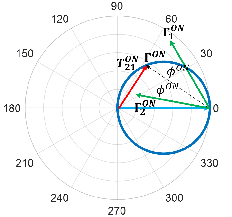
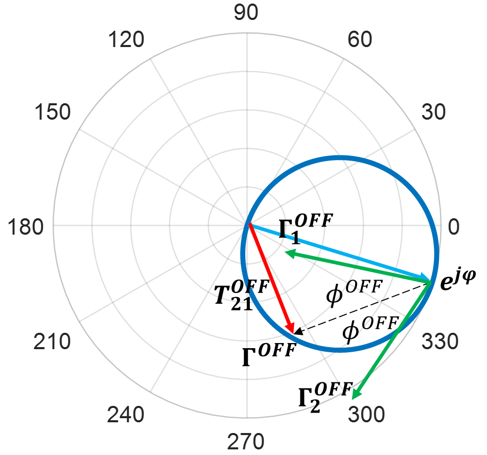
Figure 7: Geometric illustration of the relation among reflection and transmission coefficients given by (12) and (13) in asymmetric case. (a) The relations at ON state. (b) The relations at OFF state.

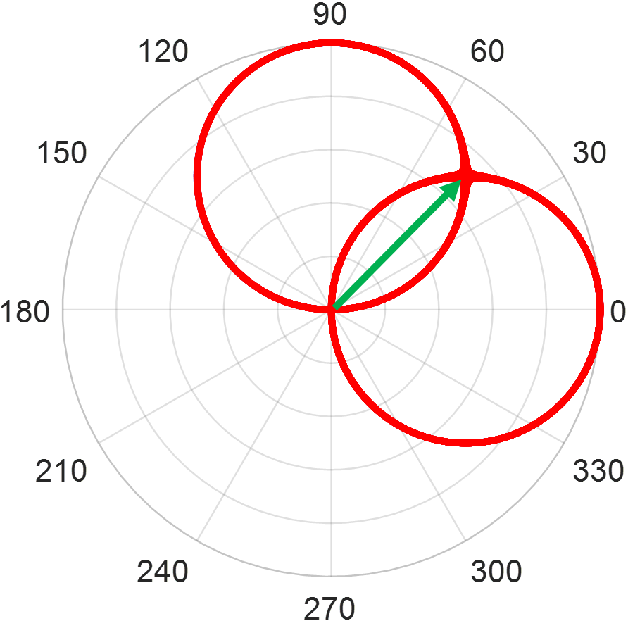
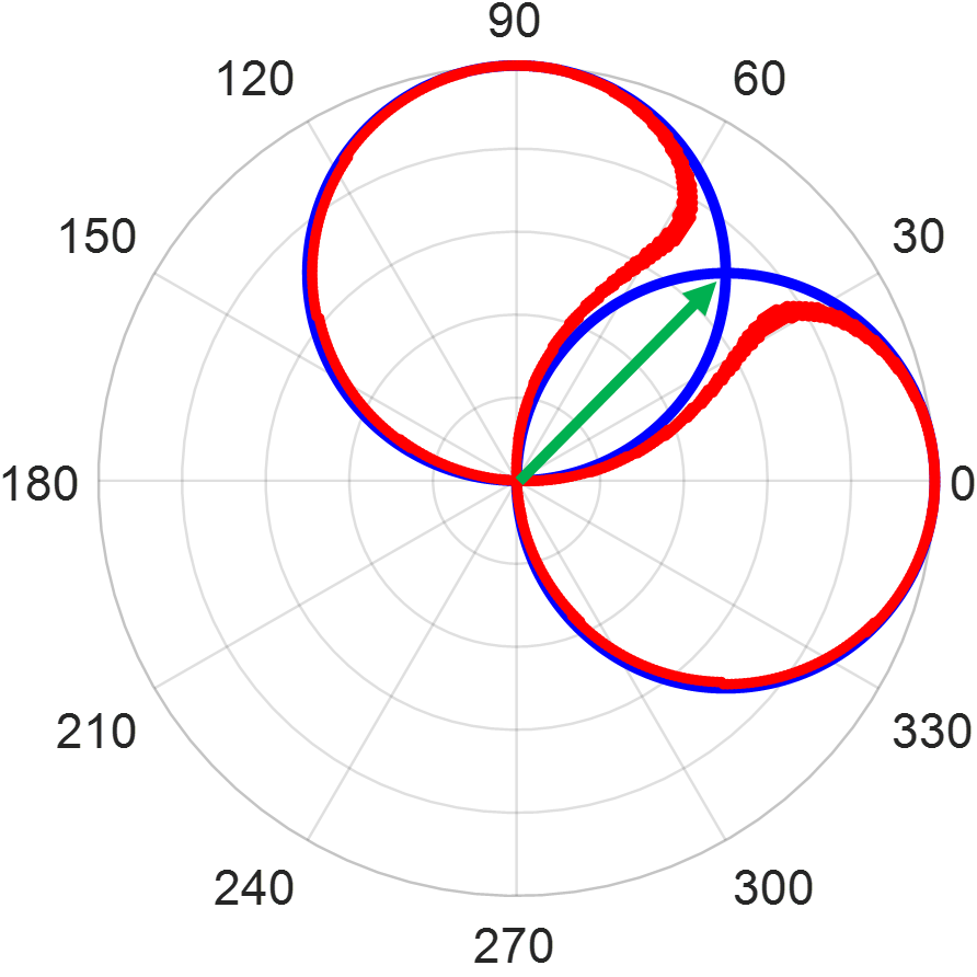
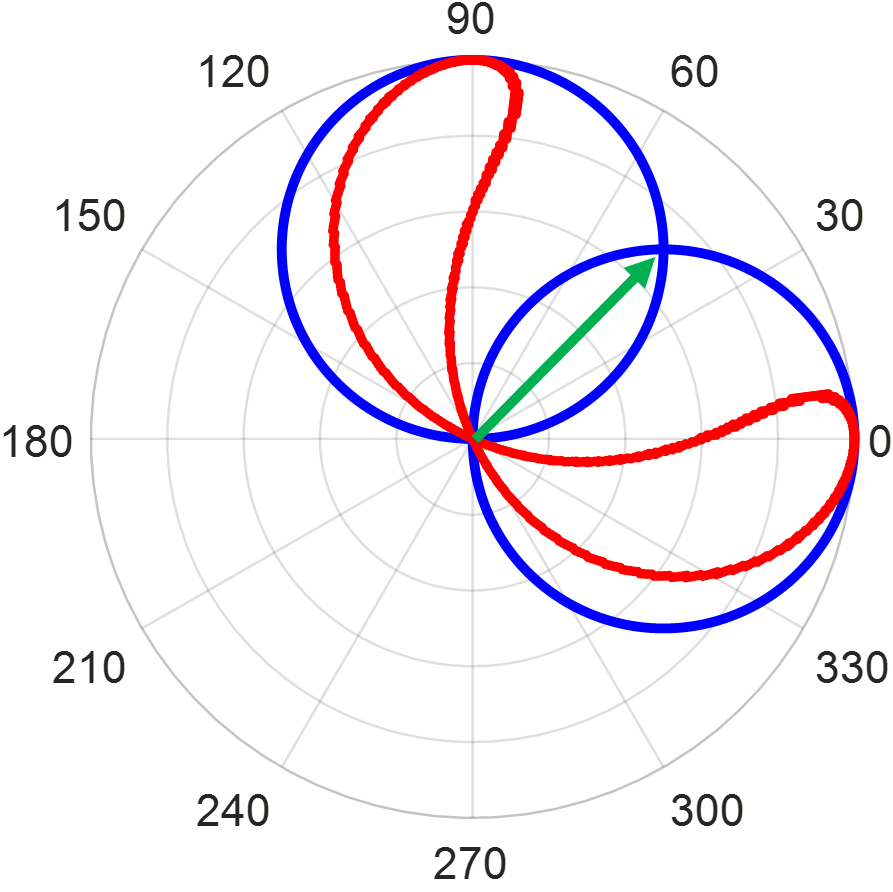
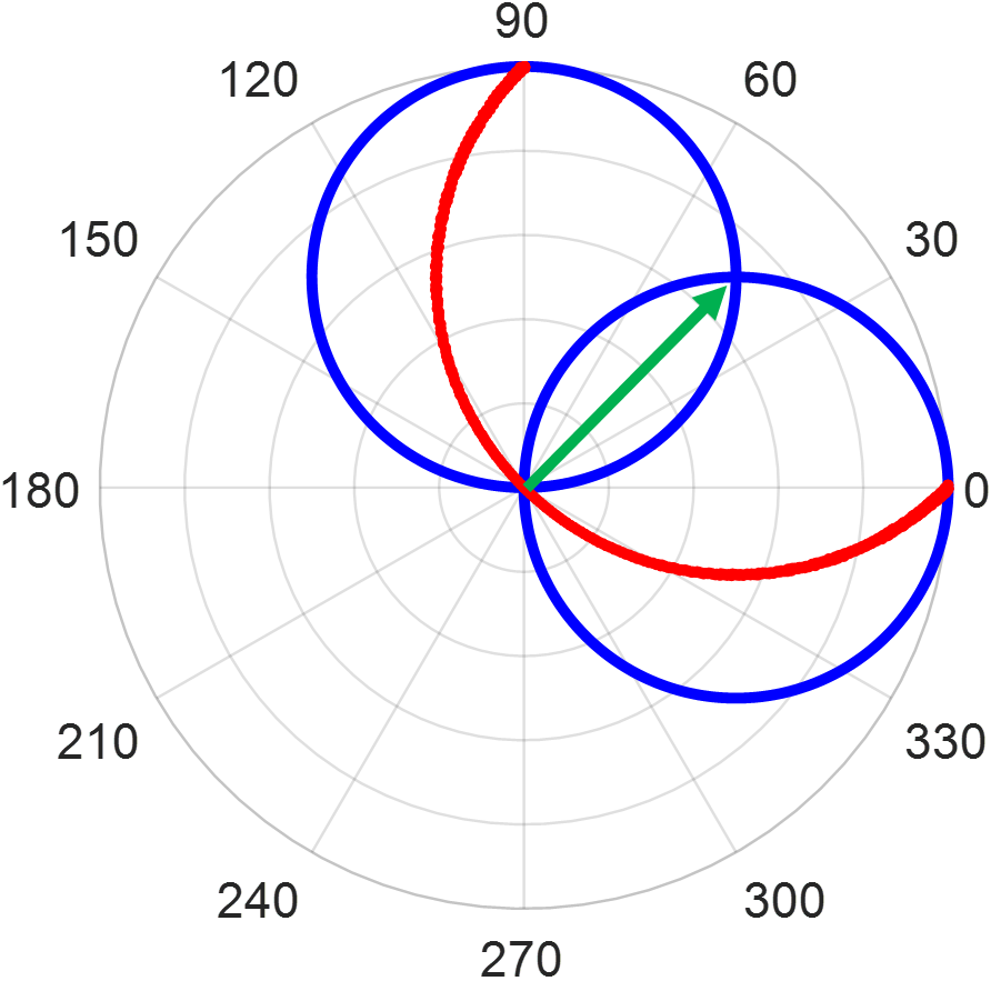
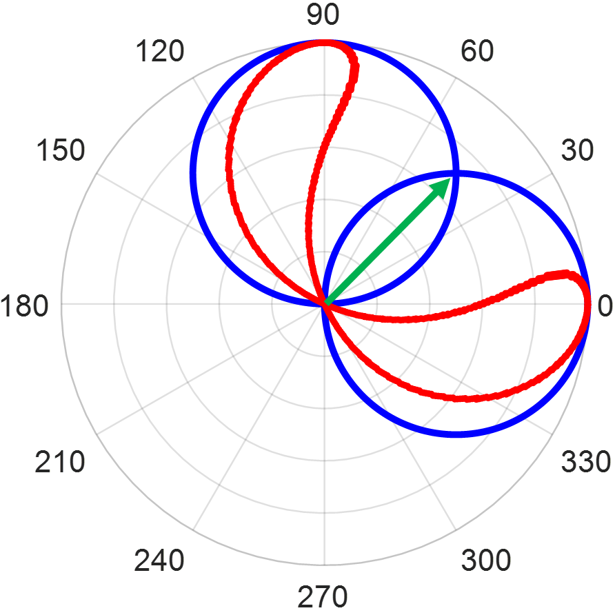
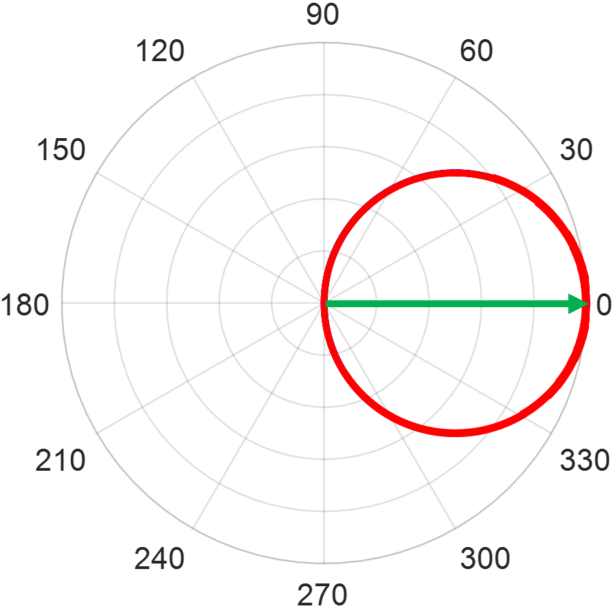
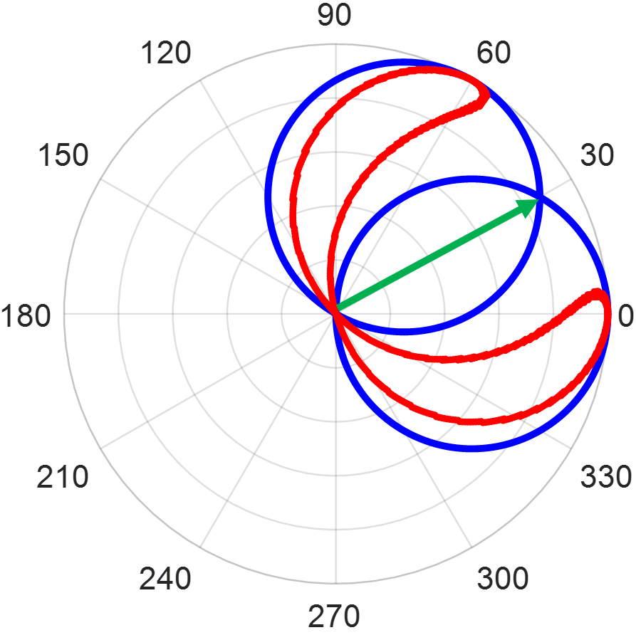
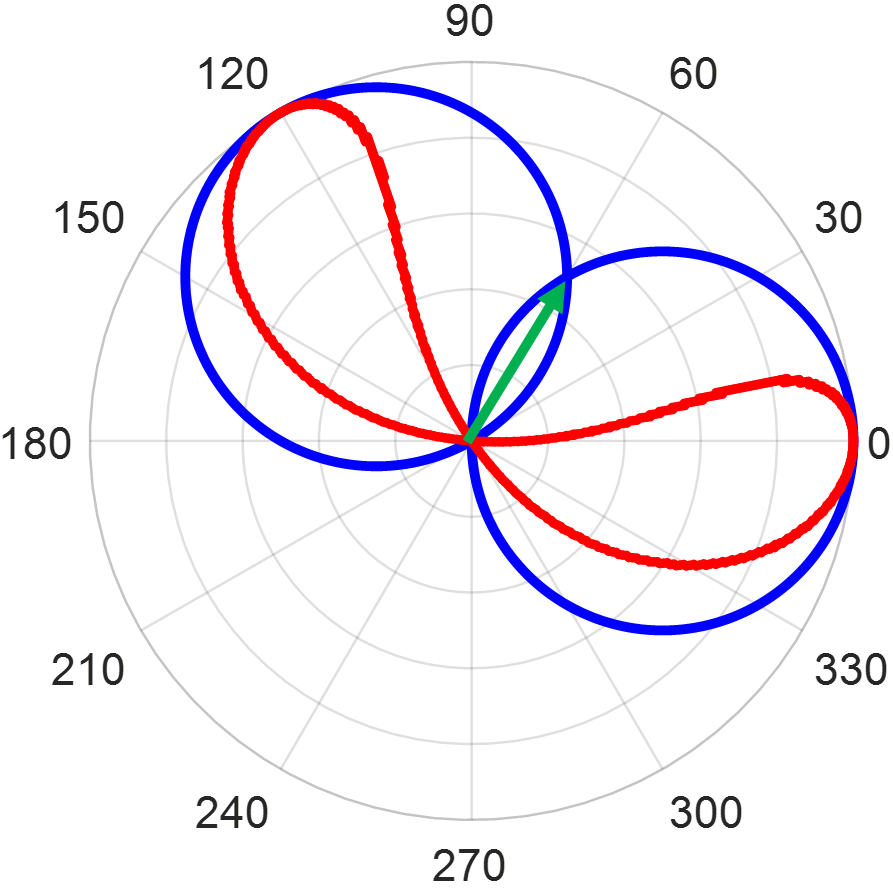
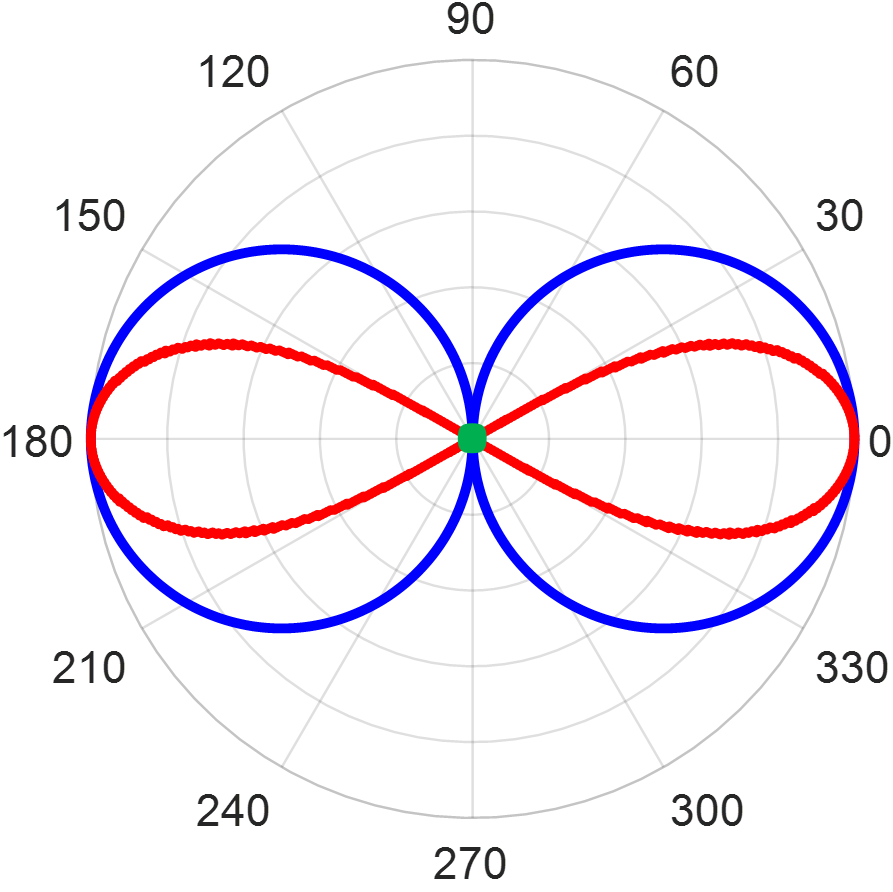
Figure 8: An illustration of the relative relation between two transmission coefficients. Green arrow: $T^{\text{ON}}_{21}$; blue circles: the circles on which $T^{\text{ON}}_{21}$ lies; red curve: the variation range of $T^{\text{OFF}}_{21}$. (a) $\theta^{\text{ON}}_{21}=\frac{\pi}{4}$, $\Delta\phi=0$. (b) $\theta^{\text{ON}}_{21}=\frac{\pi}{4}$, $\Delta\phi=\frac{\pi}{10}$. (c) $\theta^{\text{ON}}_{21}=\frac{\pi}{4}$, $\Delta\phi=\frac{\pi}{3}$. (d) $\theta^{\text{ON}}_{21}=\frac{\pi}{4}$, $\Delta\phi=\frac{\pi}{2}$. (e) $\theta^{\text{ON}}_{21}=\frac{\pi}{4}$, $\Delta\phi=\frac{2\pi}{3}$. (f) $\theta^{\text{ON}}_{21}=\frac{\pi}{4}$, $\Delta\phi=\pi$. (g) $\theta^{\text{ON}}_{21}=0$, $\Delta\phi=\frac{\pi}{3}$. (h) $\theta^{\text{ON}}_{21}=\frac{\pi}{6}$, $\Delta\phi=\frac{\pi}{3}$. (i) $\theta^{\text{ON}}_{21}=\frac{\pi}{3}$, $\Delta\phi=\frac{\pi}{3}$. (j) $\theta^{\text{ON}}_{21}=\frac{\pi}{2}$, $\Delta\phi=\frac{\pi}{3}$.

For the other state of the transmission coefficients (e.g. $T^{\text{OFF}}_{21}$), it is supposed that $T^{\text{OFF}}_{21}$ varies randomly on the Smith chart. We further suppose $T^{\text{OFF}}_{21}$ varies on the circle determined by $e^{j\varphi}$, as shown in Fig. 7(b). Similarly, the reflection coefficients is expressed as

$$\left\{\begin{array}[]{l}\Gamma^{\text{OFF}}_{1}=(T^{\text{OFF}}_{21}-e^{j\varphi})e^{-j\phi^{\text{OFF}}}\\ \Gamma^{\text{OFF}}_{2}=(T^{\text{OFF}}_{21}-e^{j\varphi})e^{j\phi^{\text{OFF}}}\\ \end{array}\right.$$ (25)

By substituting (24) and (25) into (9), the expression is finally simplified as

$$\left(T^{\text{ON}}_{21}-T^{\text{OFF}}_{21}\right)^{2} =\left(T^{\text{ON}}_{21}-1\right)^{2}+\left(T^{\text{OFF}}_{21}-e^{j\varphi}\right)^{2}$$ (26)

$$- 2\cos(\Delta\phi)\left(T^{\text{ON}}_{21}-1\right)\left(T^{\text{OFF}}_{21}-e^{j\varphi}\right),$$

where $\Delta\phi=\phi^{\text{OFF}}-\phi^{\text{ON}}$ denotes the difference between the two-state asymmetric reflection phases.

It is noted that $T^{\text{ON}}_{21}$ and $T^{\text{OFF}}_{21}$ are on the unit circles, which can be further expressed as

$$\left\{\begin{array}[]{l}T^{\text{ON}}_{21}=\left|\cos(\theta^{\text{ON}}_{21})\right|e^{j\theta^{\text{ON}}_{21}}\\ T^{\text{OFF}}_{21}=\left|\cos(\theta^{\text{OFF}}_{21}-\varphi)\right|e^{j\theta^{\text{OFF}}_{21}}\\ \end{array}\right.$$ (27)

Note that (26) has 4 parameters: $\theta^{\text{ON}}_{21}$, $\theta^{\text{OFF}}_{21}$, $\varphi$ and $\Delta\phi$.

We needs to demonstrate that $T^{\text{OFF}}_{21}$ and $T^{\text{ON}}_{21}$ lie within a circle. Theoretically, if $\theta^{\text{ON}}_{21}$, $\varphi$ and $\Delta\phi$ are given, $\theta^{\text{OFF}}_{21}$ can be solved using (26). We can then use the mathematical criterion in (11) to determine whether $T^{\text{OFF}}_{21}$ and $T^{\text{ON}}_{21}$ lie inside the same circle. However, the expression for $\theta^{\text{OFF}}_{21}$ is very complex and not intuitive. Therefore, numerical calculations are used to demonstrate the relation between $T^{\text{OFF}}_{21}$ and $T^{\text{ON}}_{21}$.

For a given group of $\theta^{\text{ON}}_{21}$ and $\Delta\phi$, a series of $\theta^{\text{OFF}}_{21}$ and $\varphi$ can be obtained that satisfy (26), and the exact value of $T^{\text{OFF}}_{21}$ depends on the specific element parameters. Without losing generality, We present several cases to demonstrate that $T^{\text{OFF}}_{21}$ is always located on or inside the circle on which $T^{\text{ON}}_{21}$ lies, as shown in Fig. 8. In Fig. 8(a)-(f), we fix $\theta^{\text{ON}}_{21}$ and thus $T^{\text{ON}}_{21}$ is also fixed. By changing $\Delta\phi$, the variation range of $T^{\text{OFF}}_{21}$ changes accordingly. If $\Delta\phi=0$ or $\pi$, $T^{\text{OFF}}_{21}$ is always on the circle of $T^{\text{ON}}_{21}$. The analytical solutions of $T^{\text{OFF}}_{21}$ for $\Delta\phi=0$ or $\pi$ are derived in the Appendix. As $\Delta\phi$ increases from $0$ to $\pi/2$, $T^{\text{OFF}}_{21}$ tend to move inside the circle, while from $\Delta\phi=\pi/2$ to $\Delta\phi=\pi$, $T^{\text{OFF}}_{21}$ tends to be on the circle again. The variation trend of $T^{\text{OFF}}_{21}$ from $\Delta\phi=\pi$ to $\Delta\phi=2\pi$ should be the same as from $\Delta\phi=\pi$ to $\Delta\phi=0$, since $\cos(2\pi-\Delta\phi)=\cos(\Delta\phi)$. Moreover, if we fix $\Delta\phi$ (e.g. $\Delta\phi=\pi/3$), the varying trend when changing $T^{\text{ON}}_{21}$ is shown in Fig. 8(c), (g)-(j). When $T^{\text{ON}}_{21}=1$, the $T^{\text{OFF}}_{21}$ is always on the circle where $T^{\text{ON}}_{21}$ varies. As $\theta^{\text{ON}}_{21}$ increases, the variation range of $T^{\text{OFF}}_{21}$ changes, but it is always within the circle on which $T^{\text{ON}}_{21}$ lies. In summary, the case studies in Fig. 8 demonstrate that for an asymmetric RTA element, $T^{\text{OFF}}_{21}$ and $T^{\text{ON}}_{21}$ are always located on or inside the same circle.

III-D Summary

TABLE I: The relations between two transmission coefficients under different conditions

Condition	Relation
Symmetric	On the circle
Asymmetric ($\Delta\phi=0$ or $\pi$)	On the circle
Asymmetric ($\left|T_{21}\right|=1$)	On the circle
Asymmetric (General situation)	Inside the circle

Based on the analysis presented above, it can be concluded that both the symmetric and asymmetric RTA elements with a single switch have their two transmission coefficients constrained by a circle. Specifically, for a lossless symmetric element, the two transmission coefficients lie on the same circle, while for a general asymmetric element, the two transmission coefficients lie inside the unit circle. There are also several special cases for asymmetric elements where the two transmission coefficients lie on the circle, namely when $\Delta\phi=0$ or $\pi$, $\left|T^{\text{ON}}_{21}\right|=1$ or $\left|T^{\text{OFF}}_{21}\right|=1$. The relations for these different scenarios are summarized in Table. I.

III-E Corollary: The Transmission Phase Difference Limit of RTA Elements

This part presents a key corollary of the proposed theory, which is the constraint on the transmission phase difference and transmission amplitudes.

As shown in Fig. 9, the transmission phase difference is defined as the included angle between the two transmission coefficients. Since the two transmission coefficents lie on or inside a unit circle, the relative phases of the two transmission coefficents can be expressed as

$$\left\{\begin{array}[]{l}\cos(\alpha^{\text{ON}})\geq\left|T^{\text{ON}}_{21}\right|\\ \cos(\alpha^{\text{OFF}})\geq\left|T^{\text{OFF}}_{21}\right|\\ \end{array}\right.$$ (28)

where $\alpha$ represents the included angle between one transmission coefficient and the diameter. Given the transmission amplitudes, the phase difference $\Delta\theta$ between the two transmission coefficients is limited by

$$\Delta\theta\leq\alpha^{\text{ON}}+\alpha^{\text{OFF}}\leq\arccos(\left|T^{\text{ON}}_{21}\right|)+\arccos(\left|T^{\text{OFF}}_{21}\right|).$$ (29)

The equal sign holds only when $T^{\text{ON}}_{21}$ and $T^{\text{OFF}}_{21}$ both lie on the circle, and they are on opposite sides of the diameter.

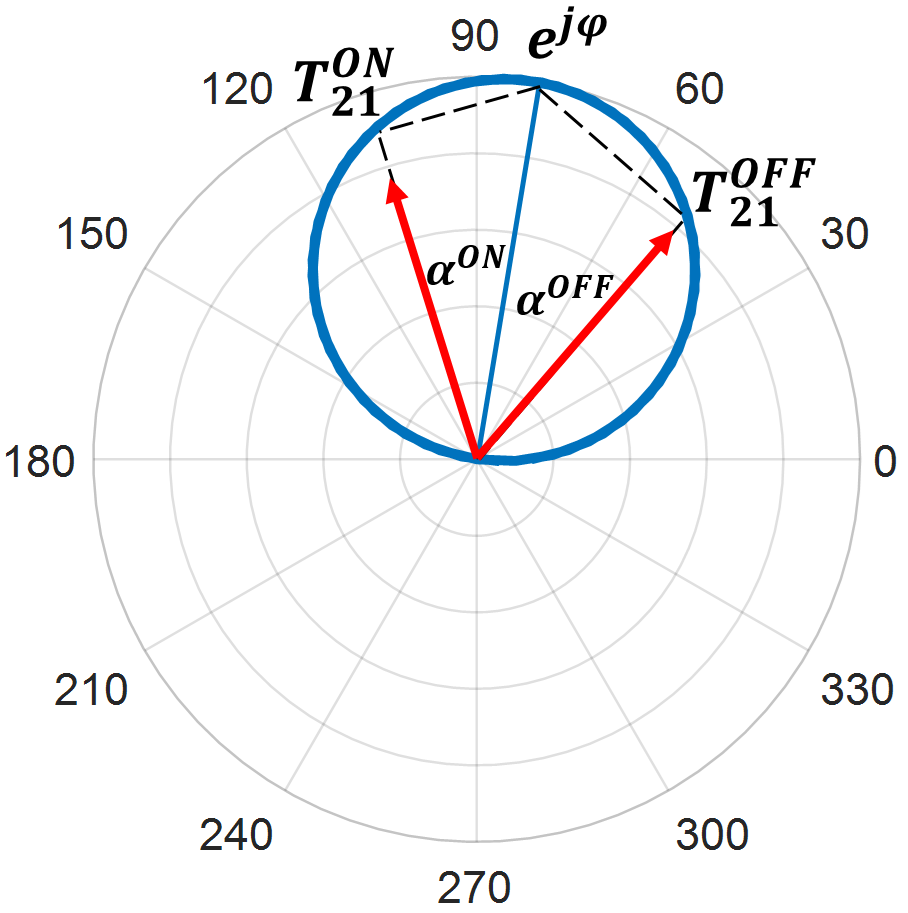
Figure 9: Geometric illustration of the relation among transmission phases and transmission amplitudes.

The maximum transmission phase difference is limited by the two transmission amplitudes, as expressed in (29). The phase difference limit (PDL) is defined as the sum of the two arccosine terms, $\arccos(\left|T^{\text{ON}}_{21}\right|)+\arccos(\left|T^{\text{OFF}}_{21}\right|)$. The relation among PDL and transmission amplitudes is plotted in Fig. 10(a). Particularly, when the two transmission amplitudes are equal, i.e., $\left|T\right|=\left|T^{\text{ON}}_{21}\right|=\left|T^{\text{OFF}}_{21}\right|$, and the relation between PDL and $\left|T\right|$ is plotted in Fig. 10(b).

The curves in Fig. 10 reveal that a single-switch RTA element cannot achieve both large phase difference and high transmission amplitudes simultaneously. For instance, to achieve high transmission amplitudes near 1, the phase difference must be close to 0. Alternatively, to achieve a phase difference of approximately 180^∘, the two transmission amplitudes should be close to 0. Moreover, to achieve a 90^∘ phase difference, at least a 3 dB amplitude loss is introduced. These results quantitatively support the findings in [33] that it is impossible to achieve high transmission efficiency with a large phase tuning range using a single-switch RTA element.

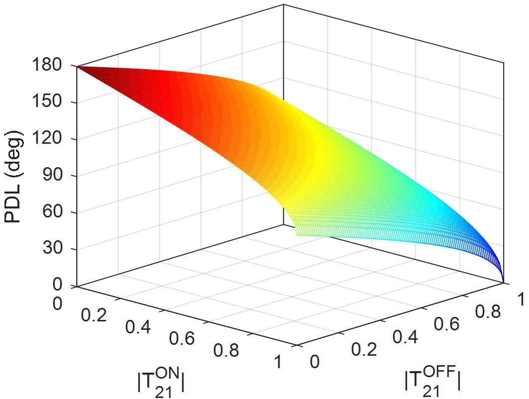
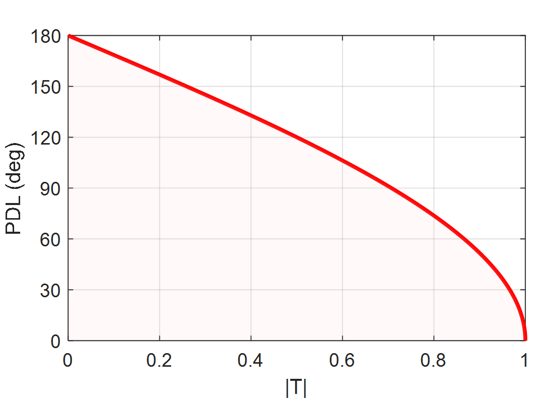
Figure 10: The relation among transmission phase difference limit and transmission amplitudes. (a) The 3-D view. (b) The 2-D view when the transmission amplitudes are equal. The feasible region is represented by the area below the curve.

IV Numerical Demonstration of the Transmission Efficiency Limit

This section presents two numerical simulation cases to validate the proposed theory. The first case involves a single-layer dipole RTA element with a single switch, while the second case features a dipole RTA element with a half ground plane. The results confirm the validity of the proposed theory, as it shows that the transmission phase difference does not break the PDL in either case.

IV-A Simulation Verification for Symmetric Structures

To confirm the conclusions regarding symmetric structures, we modeled and simulated a single-layer dipole RTA element with a single switch using Ansys HFSS 2018, as shown in Fig. 11. For the sake of brevity, the dipole is assigned as a perfect electric conductor (PEC) with no substrate loaded. The switch is modeled as $C_{\text{OFF}}=25$ fF, $L_{\text{OFF}}=30$ pH; $R_{\text{ON}}=7.8$ $\Omega$, $L_{\text{ON}}=30$ pH, with reference to [27]. The position of the switch $P_{s}$ varies from 0.2 mm to 9 mm to generate different transmission coefficients. The simulation frequency ranges from 5 GHz to 12 GHz with a step of 0.01 GHz.

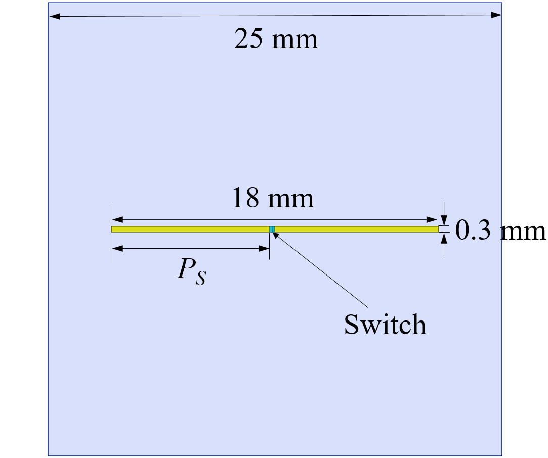
Figure 11: Top view of the single-layer dipole RTA element model with a single switch used for simulation verification in the symmetric case.

Fig. 12 shows the transmission coefficients for different switch positions. In the ON state, the transmission coefficient remains relatively constant for different $P_{s}$ values, and it is resonant at approximately 8 GHz (Fig. 12(a)). In the OFF state, the resonant frequency shifts from 10.7 GHz to approximately 8 GHz as $P_{s}$ changes from 9 mm to 0.2 mm (Fig. 12(b)). When the switch position moves toward the edge ($P_{s}$ changes toward 0.2 mm), the maximum phase difference increases, but it does not exceed $\pm$180^∘ (Fig. 12(c)).

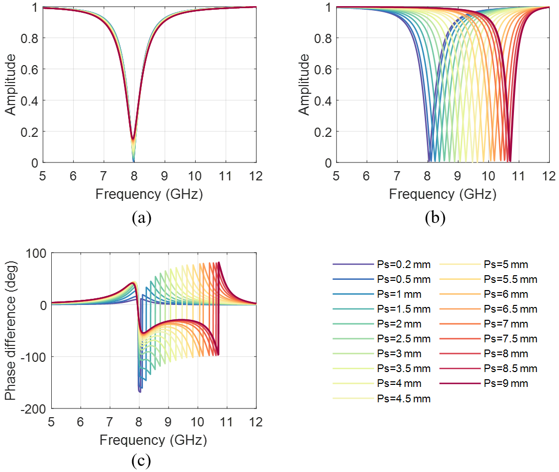
Figure 12: The transmission coefficients of the element with difference switch positions. (a) The transmission amplitudes at ON state. (b) The transmission amplitudes at OFF state. (c) The transmission phase differences.

The relationship among the phase difference and the transmission amplitudes are illustrated in Fig. 13. The actual phase differences at different frequencies with varying switch positions are plotted alongside the calculated PDL curve based on the transmission amplitudes in Figure 13(a)-(b). The results show that the actual phase differences remain below the PDL curve and do not break it. Moreover, at certain switch positions, there are frequency points where $\left|T\right|=\left|T^{\text{ON}}_{21}\right|=\left|T^{\text{OFF}}_{21}\right|$, and the relationship between $\left|T\right|$ and the phase difference is depicted in Fig. 13(c). The findings confirm that for any given $\left|T\right|$ value, the corresponding $\Delta\theta$ is near the PDL curve without breaking it, which supports the conclusion that the two transmission coefficients are on the circle for symmetric structures, as discussed in Section III. The observed error is mainly due to the loss of the switch.

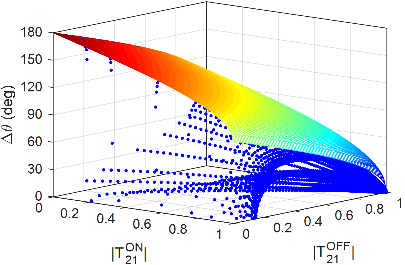
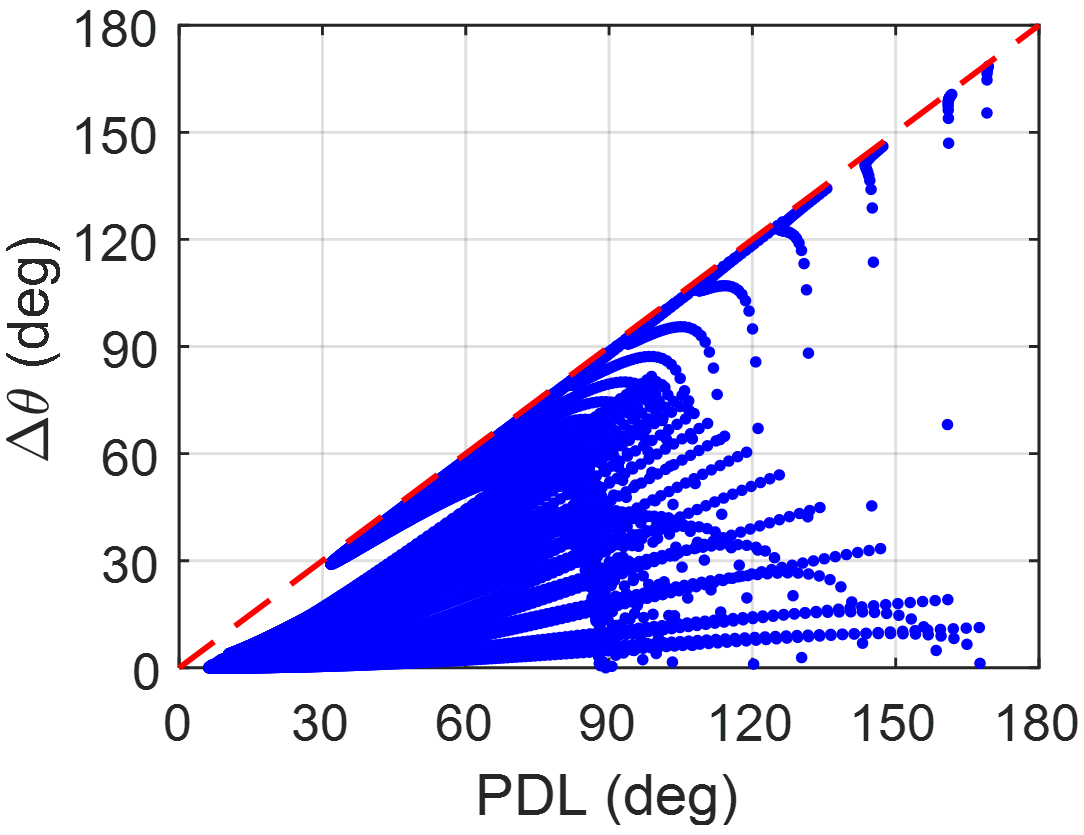
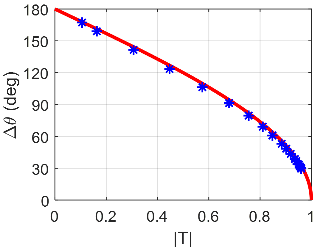
Figure 13: The simulated transmission phase difference and transmission amplitudes of the symmetric RTA element, with blue dots representing a series of simulated transmission coefficients. (a) The 3-D view. (b) The 2-D view of the relationship between $\Delta\theta$ and PDL. (b) The 2-D view when $\left|T\right|=\left|T^{\text{ON}}_{21}\right|=\left|T^{\text{OFF}}_{21}\right|$.

In summary, the simulation example presented in this study shows that the transmission phase is limited by the transmission amplitudes.

IV-B Simulation Verification for Asymmetric Structures

To demonstrate the effect of asymmetry, a half ground plane is introduced beneath the dipole, breaking the symmetric condition, as shown in Fig. 14. The simulation is conducted in Ansys HFSS 2018, where the metal is assigned as PEC and no substrate is introduced for brevity. An ideal switch without resistance is used with the following parameters: $C_{\text{OFF}}=25$ fF, $L_{\text{OFF}}=30$ pH; $L_{\text{ON}}=30$ pH. The switch position $P_{s}$ ranges from 1 mm to 11 mm, and the simulation frequency ranges from 5 GHz to 12 GHz with a step of 0.01 GHz.

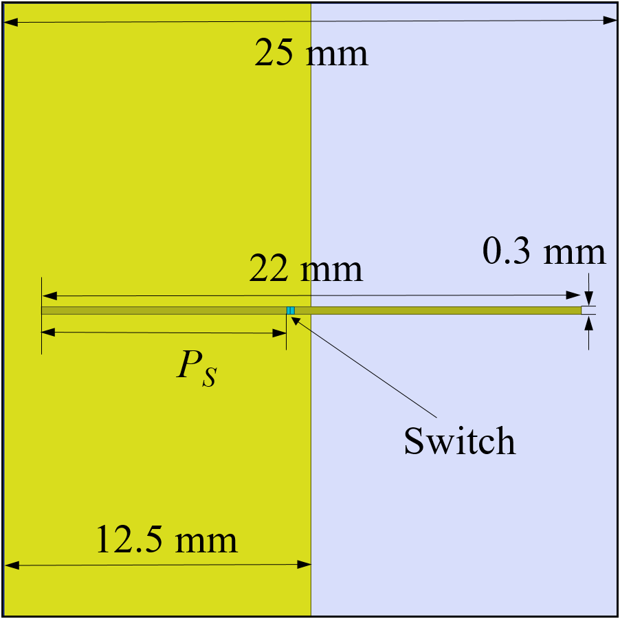
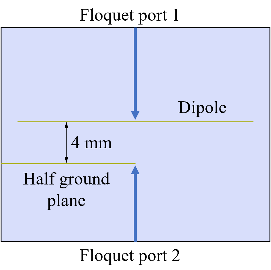
Figure 14: Simulation model of an asymmetric RTA element with a dipole and a half ground plane. (a) Top view. (b) Side view.

To begin with, we want to confirm that the designed structure can produce asymmetric reflection coefficients. As illustrated in Fig. 7, the asymmetric reflection phase is defined as $\phi=(\theta_{1}-\theta_{2})/2$, where $\theta_{1}$ and $\theta_{2}$ represent the reflection phases from two ports, respectively. As depicted in Fig. 15(a)-(b), the asymmetric reflection phases are generally neither 0 nor $\pi$ under both switch states, which confirms that the reflection coefficients from the two ports are asymmetric. Moreover, Fig. 15(c) shows the differences between the two asymmetric reflection phases, denoted by $\Delta\phi$. From 5 GHz to 9 GHz, $\Delta\phi$ is neither 0 nor $\pi$, indicating that the two transmission coefficients should be within the circle when the amplitudes are not 1.

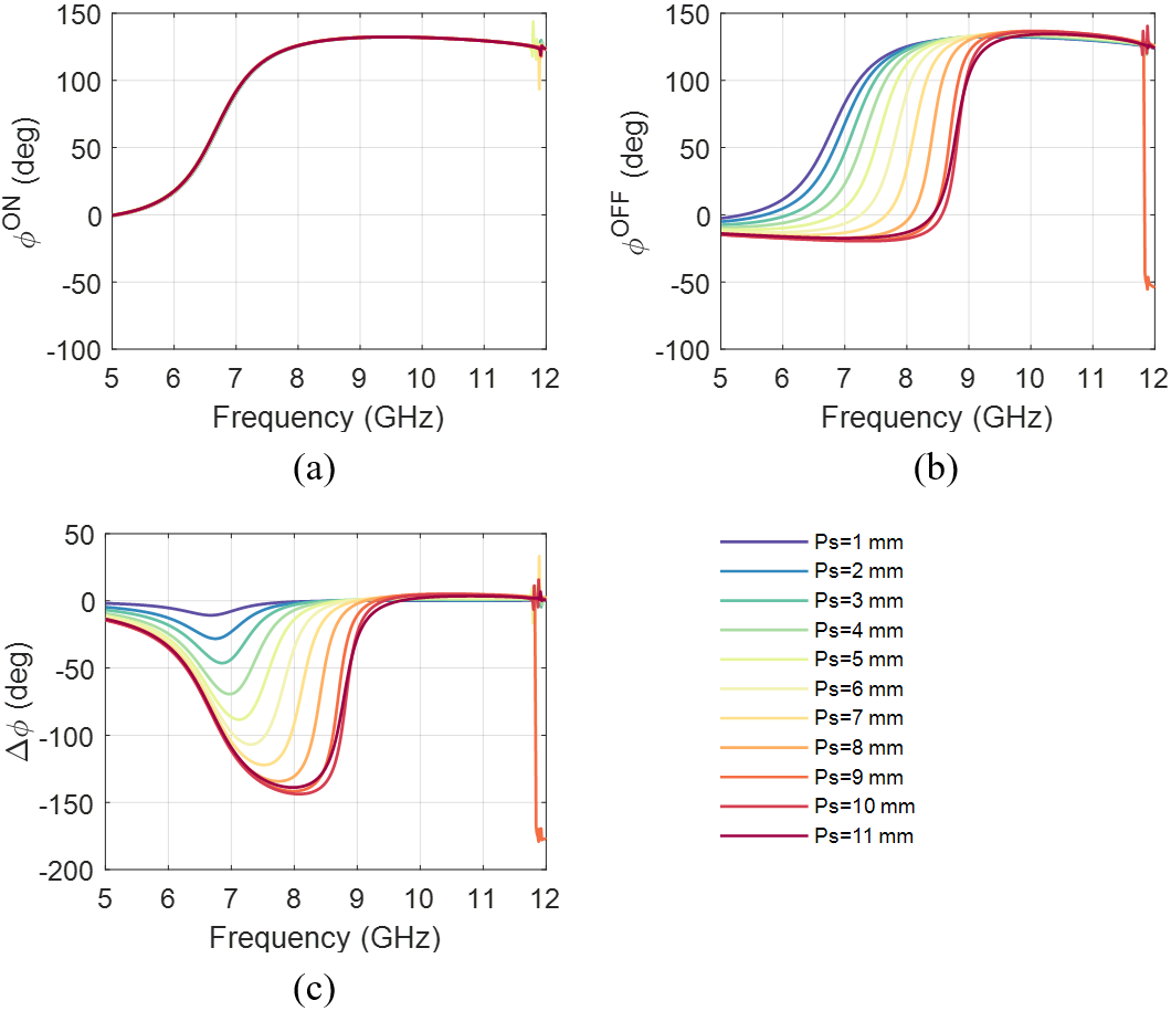
Figure 15: The simulated asymmetric reflection phases and their differences of the asymmetric structure. (a) The asymmetric reflection phases at ON state. (b) The asymmetric reflection phases at OFF state. (c) The differences between asymmetric reflection phases.

Fig. 16 illustrates the transmission coefficients of the asymmetric RTA element under both switch states. At the ON state, the dipole induces a resonant frequency around 6.6 GHz. By adjusting the position of the switch at the OFF state, the transmission coefficients shift. As the switch moves closer to the edge of the dipole, the resonant frequency approaches 6.6 GHz. Additionally, the transmission phase differences between the two states vary, but they remain within the $\pm$180^∘ phase limit.

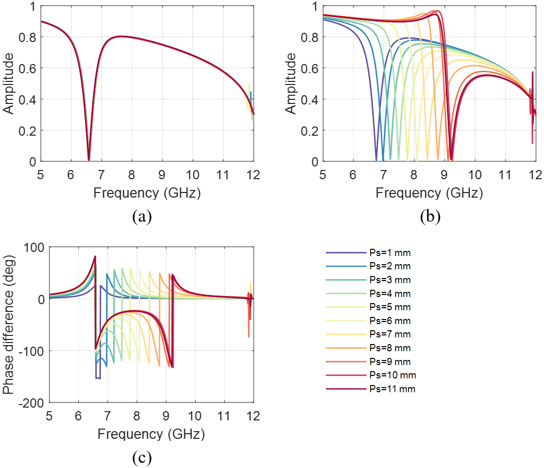
Figure 16: The transmission coefficients of the asymmetric element with difference switch positions. (a) The transmission amplitudes at ON state. (b) The transmission amplitudes at OFF state. (c) The transmission phase differences.

Fig. 17(a)-(b) show the transmission amplitudes and phase differences. It is observed that, for all given transmission amplitudes, the phase differences remain within the PDL. Additionally, a special case is analyzed, where the two transmission amplitudes are equal, as shown in Fig. 17(c). It is found that the phase differeces are also within the maximum limit determined by the transmission amplitudes. Notably, some of the phase differeces can nearly reach the PDL, such as the point with $\Delta\theta\approx 150^{\circ}$, indicating that the two transmission coefficients lie on the circle. This is because $\Delta\phi$ is close to 0, and it has been demonstrated in the Appendix that the two transmission coefficients should lie on the unit circle. Furthermore, some points in Fig. 17(c) do not reach the PDL, indicating that the two transmission coefficients are within the unit circle. These observations varify that, for asymmetric structures, the two transmission coefficients should lie on or within the unit circle.

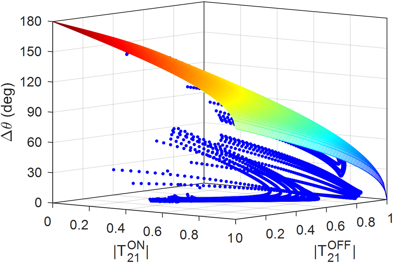
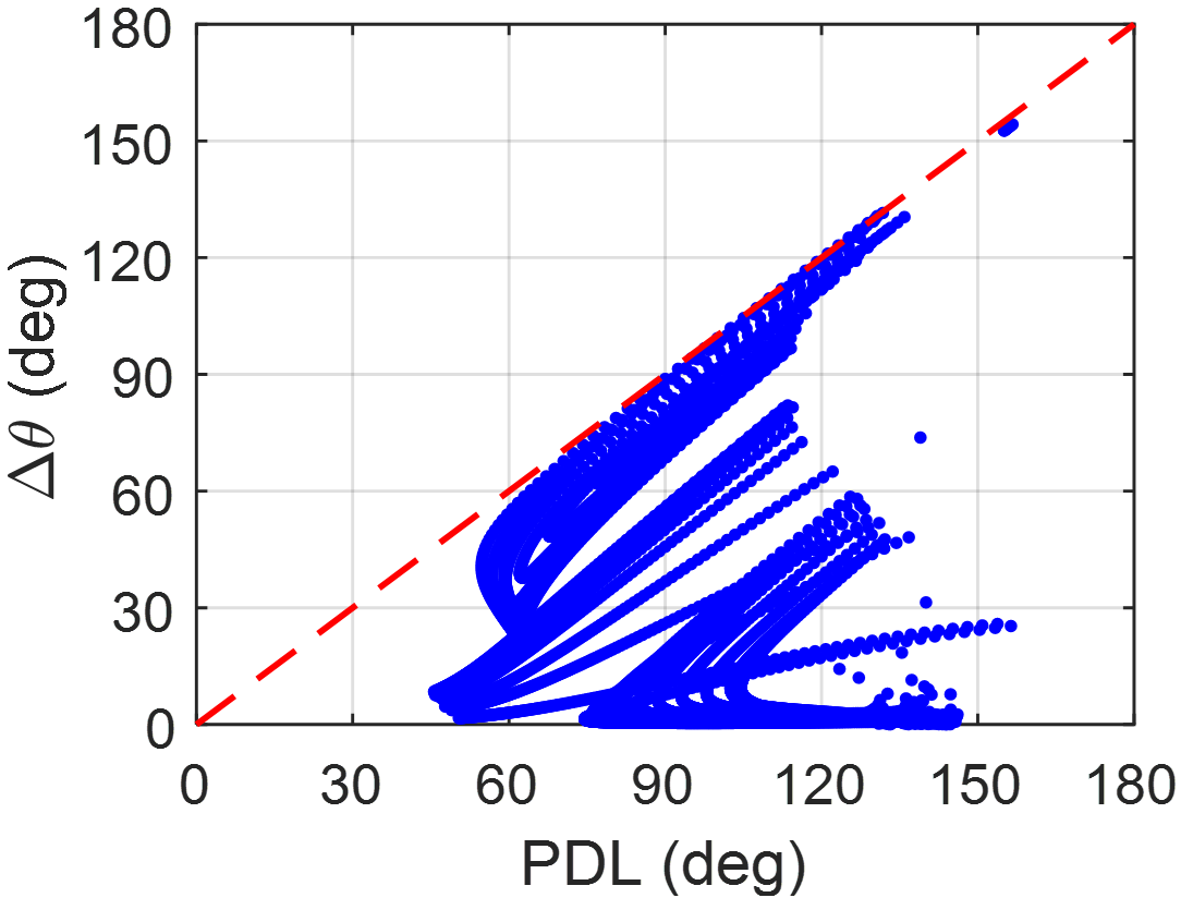
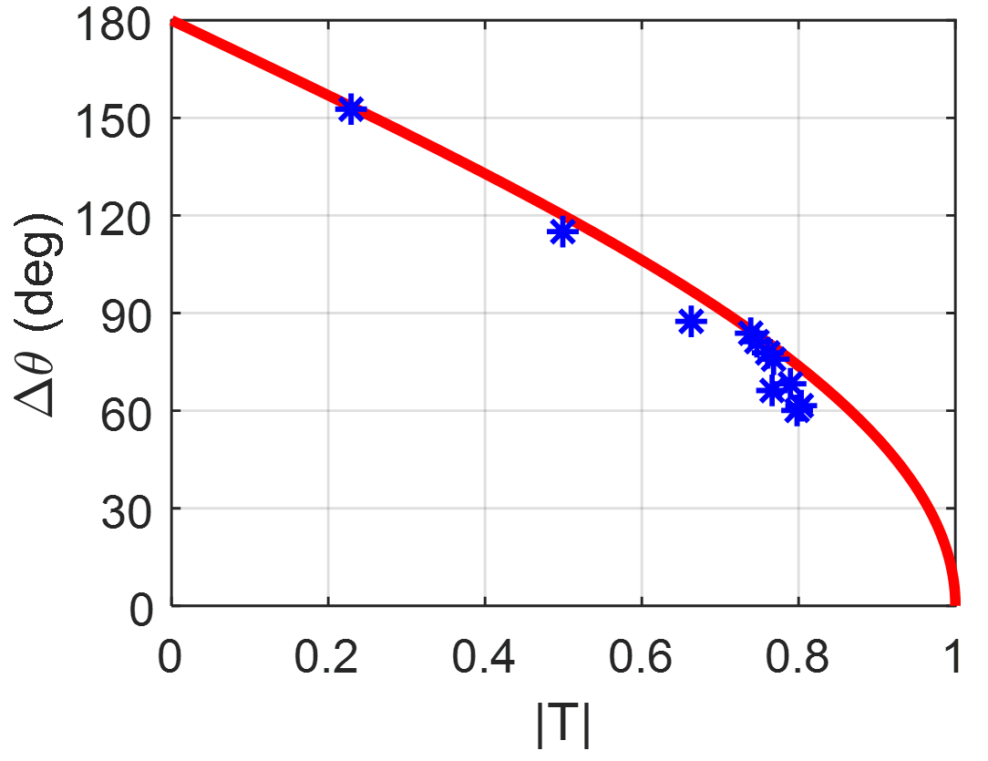
Figure 17: The transmission phase difference and transmission amplitudes of the simulated asymmetric RTA element. The blue dots are a series of simulated transmission coefficients. (a) The 3-D view. (b) The 2-D view of the relation between $\Delta\theta$ and PDL. (b) The 2-D view when $\left|T\right|=\left|T^{\text{ON}}_{21}\right|=\left|T^{\text{OFF}}_{21}\right|$.

V Conclusion

This paper presents a theory on the transmission efficiency limit of single-switch RTA elements. The RTA element can be modeled as a three-port microwave network. The study uses analytical derivations, geometric representation, and numerical simulations to show that the transmission coefficients under two states should be on or inside a unit circle with a diameter of 1 on the Smith chart. Additionally, it is found that the transmission phase difference has an upper limit determined by the transmission amplitudes. This result provides solid evidence that it is not feasible to achieve both high transmission amplitudes and large phase tuning range using a single-switch RTA element.

These conclusions are not limited to single-switch RTA elements, but also apply to other reconfigurable elements with the same three-port network topology. Examples of such elements include single-switch RRA elements with polarization conversion, the single-switch RTA elements based on near-field feeding method, planar reconfigurable elements with a single switch based on transmission-line feeding method, and so on.

This appendix analytically demonstrates that if $\Delta\phi=0$ or $\pi$, then $T^{\text{OFF}}_{21}$ should lie on the same circle as $T^{\text{ON}}_{21}$.

Starting from (26), let us consider the case where $\Delta\phi=0$. This simplifies (26) to

$$\left(T^{\text{ON}}_{21}-T^{\text{OFF}}_{21}\right)^{2}=\left(T^{\text{ON}}_{21}-T^{\text{OFF}}_{21}-1+e^{j\varphi}\right)^{2}.$$ (30)

This equation has two sets of solutions.

1. $T^{\text{ON}}_{21}-T^{\text{OFF}}_{21}=T^{\text{ON}}_{21}-T^{\text{OFF}}_{21}-1+e^{j\varphi}$, which simplifies to $e^{j\varphi}=1$. This means that $T^{\text{OFF}}_{21}$ varies on the same circle as $T^{\text{ON}}_{21}$.

2. $T^{\text{ON}}_{21}-T^{\text{OFF}}_{21}=-T^{\text{ON}}_{21}+T^{\text{OFF}}_{21}+1-e^{j\varphi}$. This can be rearranged as

   $$T^{\text{ON}}_{21}-T^{\text{OFF}}_{21}=\frac{1-e^{j\varphi}}{2}.$$ (31)

   Based on (27), $T^{\text{ON}}_{21}$ can be written as

   $$T^{\text{ON}}_{21}=\frac{e^{j2\theta^{\text{ON}}_{21}}+1}{2}.$$ (32)

   Substituting (32) into (31), $T^{\text{OFF}}_{21}$ is expressed as

   $$T^{\text{OFF}}_{21}=\frac{e^{j2\theta^{\text{ON}}_{21}}+e^{j\varphi}}{2}.$$ (33)

   Geometrically, this means that $T^{\text{OFF}}_{21}$ varies on the circle with diameter $e^{j2\theta^{\text{ON}}_{21}}$, on which $T^{\text{ON}}_{21}$ also lies (when $e^{j\varphi}=1$), as shown in Fig. 18. This demonstrates that $T^{\text{ON}}_{21}$ and $T^{\text{OFF}}_{21}$ lie on the same circle.

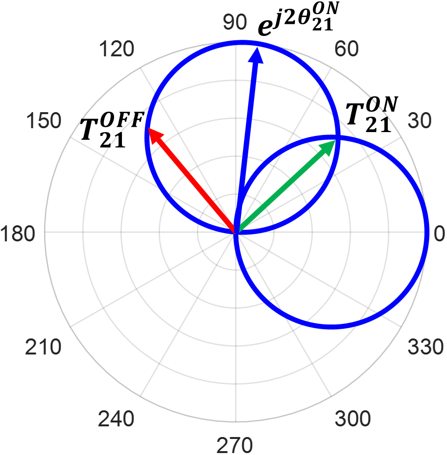
Figure 18: Geometric illustration of (33) and (37). $T^{\text{OFF}}_{21}$ lies on circle with diameter $e^{j2\theta^{\text{ON}}_{21}}$, on which $T^{\text{ON}}_{21}$ also lies.

Then consider the case where $\Delta\phi=\pi$. (26) simplifies as

$$\left(T^{\text{ON}}_{21}-T^{\text{OFF}}_{21}\right)^{2}=\left(T^{\text{ON}}_{21}+T^{\text{OFF}}_{21}-1-e^{j\varphi}\right)^{2}.$$ (34)

This equation has two sets of solutions.

1. $T^{\text{ON}}_{21}-T^{\text{OFF}}_{21}=T^{\text{ON}}_{21}+T^{\text{OFF}}_{21}-1-e^{j\varphi}$, which leads to

   $$T^{\text{OFF}}_{21}=\frac{1+e^{j\varphi}}{2}.$$ (35)

   Obviously, $T^{\text{OFF}}_{21}$ lies on the circle with diameter 1, which implies that $T^{\text{ON}}_{21}$ and $T^{\text{OFF}}_{21}$ are on the same circle.

2. $T^{\text{ON}}_{21}-T^{\text{OFF}}_{21}=-T^{\text{ON}}_{21}-T^{\text{OFF}}_{21}+1+e^{j\varphi}$, which leads to

   $$T^{\text{ON}}_{21}=\frac{1+e^{j\varphi}}{2}.$$ (36)

   Inserting (32) into (36), it is found that

   $$e^{j\varphi}=e^{j2\theta^{\text{ON}}_{21}},$$ (37)

   which means $T^{\text{OFF}}_{21}$ varies on the circle with a diameter of $e^{j2\theta^{\text{ON}}_{21}}$, on which $T^{\text{ON}}_{21}$ also lies, as shown in Fig. 18. Thus, $T^{\text{ON}}_{21}$ and $T^{\text{OFF}}_{21}$ also lie on the same circle in this case.

References

- [1] P. Nayeri, F. Yang, and A. Z. Elsherbeni, Reflectarray Antennas: Theory, Designs and Applications. New York, NY, USA: Wiley, 2018.
- [2] S. V. Hum and J. Perruisseau-Carrier, “Reconfigurable reflectarrays and array lenses for dynamic antenna beam control: A review,” IEEE Trans. Antennas Propag., vol. 62, no. 1, pp. 183–198, Jan. 2014.
- [3] P. Nayeri, F. Yang, and A. Elsherbeni, “Beam scanning reflectarray antennas: A technical overview and state of the art,” IEEE Antennas Propag. Mag., vol. 57, no. 4, pp. 32–47, Aug. 2015.
- [4] C. Liu, F. Yang, S. Xu, and M. Li, “Reconfigurable metasurface: A systematic categorization and recent advances,” arXiv preprint arXiv:2301.00593, 2023.
- [5] A. H. Abdelrahman, A. Z. Elsherbeni, and F. Yang, “Transmission phase limit of multilayer frequency selective surfaces for transmitarray designs,” IEEE Trans. Antennas Propag., vol. 62, no. 2, pp. 690–697, Feb. 2014.
- [6] F. Yang, R. Deng, S. Xu, and M. Li, “Design and experiment of a near-zero-thickness high-gain transmit-reflect-array antenna using anisotropic metasurface,” IEEE Trans. Antennas Propag., vol. 66, no. 6, pp. 2853–2861, Mar. 2018.
- [7] H. Yang et al., “A study of phase quantization effects for reconfigurable reflectarray antennas,” IEEE Antennas Wireless Propag. Lett., vol. 16, no. 5, pp. 302-305, Mar. 2017.
- [8] E. Carrasco, M. Barba, and J. A. Encinar, “X-band reflectarray antenna with switching-beam using pin diodes and gathered elements,” IEEE Trans. Antennas Propag., vol. 60, no. 12, pp. 5700–5708, Dec. 2012.
- [9] O. Bayraktar, O. A. Civi, and T. Akin, “Beam switching reflectarray monolithically integrated with RF MEMS switches,” IEEE Trans. Antennas Propag., vol. 60, no. 2, pp. 854–862, Feb. 2012.
- [10] H. Yang et al., “A 1-bit reconfigurable reflectarray antenna: design, optimization, and experiment,” IEEE Trans. Antennas Propag., vol. 64, no. 6, pp. 2246-2254, June 2016.
- [11] H. Zhang, X. Chen, Z. Wang, Y. Ge and J. Pu, “A 1-bit electronically reconfigurable reflectarray antenna in X band,” IEEE Access, vol. 7, pp. 66567-66575, 2019.
- [12] X. Pan, F. Yang, S. Xu and M. Li, “A 10240-element reconfigurable reflectarray with fast steerable monopulse patterns,” IEEE Trans. Antennas Propag., vol. 69, no. 1, pp. 173-181, Jan. 2021.
- [13] H. Kamoda, T. Iwasaki, J. Tsumochi, T. Kuki and O. Hashimoto, “60-GHz electronically reconfigurable large reflectarray using single-bit phase shifters,” IEEE Trans. Antennas Propag., vol. 59, no. 7, pp. 2524-2531, July 2011.
- [14] X. Pan, S. Wang, G. Li, S. Xu and F. Yang, “On-chip reconfigurable reflectarray for 2-D beam-steering at W-band,” in 2018 IEEE MTT-S International Wireless Symposium (IWS), 2018, pp. 1-4.
- [15] X. Pan, F. Yang and X. Nie, “Analysis and design of THz 1-bit RRA element with series inductance,” in 2021 IEEE International Symposium on Antennas and Propagation and USNC-URSI Radio Science Meeting (APS/URSI), 2021.
- [16] J. Han, L. Li, G. Liu, Z. Wu and Y. Shi, “A wideband 1 bit reconfigurable beam-scanning reflectarray: Design fabrication and measurement,” IEEE Antennas Wireless Propag. Lett., vol. 18, no. 6, pp. 1268-1272, Jun. 2019.
- [17] B. J. Xiang, X. Dai, and K. M. Luk, “A wideband low-cost reconfigurable reflectarray antenna with 1-bit resolution,” IEEE Trans. Antennas Propag., vol. 70, no. 9, pp. 7439-7447, Sept. 2022.
- [18] H. Yang et al., “A 1600-element dual-frequency electronically reconfigurable reflectarray at X/Ku-band,” IEEE Trans. Antennas Propag., vol. 65, no. 6, pp. 3024-3032, June 2017.
- [19] C. Liu, F. Yang, M. Li, and S. Xu, “Deep-learning-empowered inverse design for freeform reconfigurable metasurfaces,” arXiv preprint arXiv:2211.08296, 2022.
- [20] C. Liu et al., “A radiation viewpoint of reconfigurable reflectarray elements: Performance limit, evaluation method and design process,” arXiv preprint arXiv:2211.08632, 2023.
- [21] A. Clemente, L. Dussopt, R. Sauleau, P. Potier, and P. Pouliguen, “1-bit reconfigurable unit cell based on PIN diodes for transmit-array applications in X-band,” IEEE Trans. Antennas Propag., vol. 60, no. 5, pp. 2260–2269, Mar. 2012.
- [22] A. Clemente, L. Dussopt, R. Sauleau, P. Potier and P. Pouliguen, “Wideband 400-element electronically reconfigurable transmitarray in X band,” IEEE Trans. Antennas Propag., vol. 61, no. 10, pp. 5017-5027, Oct. 2014.
- [23] C. Huang, W. Pan, X. Ma and X. Luo, “1-bit reconfigurable circularly polarized transmitarray in X-band,” IEEE Antennas Wireless Propag. Lett., vol. 13, pp. 448-451, 2016.
- [24] L. Di Palma, A. Clemente, L. Dussopt, R. Sauleau, P. Potier and P. Pouliguen, “Circularly-polarized reconfigurable transmitarray in Ka-band with beam scanning and polarization switching capabilities,” IEEE Trans. Antennas Propag., vol. 65, no. 2, pp. 529-540, Feb. 2017.
- [25] M. Wang et al., “Design and measurement of a Ku-band pattern-reconfigurable array antenna using 16 O-slot patch elements with p-i-n diodes,” IEEE Antennas Wireless Propag. Lett., vol. 19, no. 12, pp. 2373-2377, Dec. 2020.
- [26] M. Wang, S. Xu, F. Yang and M. Li, “Design and measurement of a 1-bit reconfigurable transmitarray with subwavelength H-shaped coupling slot elements,” IEEE Trans. Antennas Propag., vol. 67, no. 5, pp. 3500-3504, May 2019.
- [27] Y. Wang, S. Xu, F. Yang and M. Li, “A novel 1 bit wide-angle beam scanning reconfigurable transmitarray antenna using an equivalent magnetic dipole element,” IEEE Trans. Antennas Propag., vol. 68, no. 7, pp. 5691-5695, July 2020.
- [28] H. Yu, J. Su, Z. Li and F. Yang, “A novel wideband and high-efficiency electronically scanning transmitarray using transmission metasurface polarizer,” IEEE Trans. Antennas Propag., vol. 70, no. 4, pp. 3088-3093, Apr. 2022.
- [29] Y. Xiao, F. Yang, S. Xu, M. Li, K. Zhu and H. Sun, “Design and implementation of a wideband 1-bit transmitarray based on a Yagi-Vivaldi unit cell,” IEEE Trans. Antennas Propag., vol. 69, no. 7, pp. 4229-4234, Jul. 2021.
- [30] B. D. Nguyen and C. Pichot, “Unit-cell loaded with PIN diodes for 1-bit linearly polarized reconfigurable transmitarrays,” IEEE Antennas Wireless Propag. Lett., vol. 18, no. 1, pp. 98-102, Jan. 2019.
- [31] C.-W. Luo, G. Zhao, Y.-C. Jiao, G.-T. Chen, and Y.-D. Yan, “Wideband 1 bit reconfigurable transmitarray antenna based on polarization rotation element,” IEEE Antennas Wireless Propag. Lett., vol. 20, no. 5, pp. 798–802, May 2021.
- [32] X. Wang, P. -Y. Qin, A. T. Le, H. Zhang, R. Jin and Y. Jay Guo, “Beam scanning transmitarray employing reconfigurable dual-layer huygens element,” IEEE Trans. Antennas Propag., vol. 70, no. 9, pp. 7491–7500, Sep. 2022.
- [33] C. Liu, Y. Wu, F. Yang, S. Xu and M. Li, “Is it possible to design a 1-bit reconfigurable transmitarray element with a single switch?” IEEE Antennas Wirel. Propag. Lett., in press.
- [34] D. M. Pozar, Microwave Engineering, New York, NY, USA:Wiley, 2011.