Existence proof of librational invariant
tori in an averaged model
of HD60532 planetary system

Abstract

We investigate the long-term dynamics of HD60532, an extrasolar system hosting two giant planets orbiting in a 3:1 mean motion resonance. We consider an average approximation at order one in the masses which results (after the reduction of the constants of motion) in a resonant Hamiltonian with two libration angles. In this framework, the usual algorithms constructing the Kolmogorov normal form approach do not easily apply and we need to perform some untrivial preliminary operations, in order to adapt the method to this kind of problems. First, we perform an average over the fast angle of libration which provides an integrable approximation of the Hamiltonian. Then, we introduce action-angle variables that are adapted to such an integrable approximation. This sequence of preliminary operations brings the Hamiltonian in a suitable form to successfully start the Kolmogorov normalization scheme. The convergence of the KAM algorithm is proved by applying a technique based on a computer-assisted proof. This allows us to reconstruct the quasi-periodic motion of the system, with initial conditions that are compatible with the observations.

1 Introduction

The discovery of the first multiple-planet extrasolar system, $\upsilon$ Andromedæ (see [3]), immediately raised the question of its stability, notably from a dynamical system point of view. Nowadays more than 800 multiple-planet extrasolar systems have been discovered, making the question even more relevant.

Typically, these systems have been numerically investigated as a sort of inverse problem, prescribing their stability in order to determine ranges of possible values of a few orbital elements which are unknown or poorly known (e.g., inclinations and longitudes of the nodes). The numerical investigations of the dynamical behavior of many interesting extrasolar planetary systems have been done complementing long-term integrations (see, e.g., [28] and [7]) with refined numerical techniques, like for instance the frequency analysis method or the MEGNO chaos indicator (see, e.g., [20] and [37], respectively).

Perturbation theory allows to complement the numerical investigations with rigorous analytic results. Normal form methods have a long-standing tradition and their applications to problems that are relevant in Celestial Mechanics have grown more and more with the development of the algebraic manipulators (for an introduction to the main concepts of this kind of software see, e.g., [14]). Therefore, in such a framework the study of extrasolar planetary systems (in particular, of their secular dynamics) started very soon (see, e.g., [29]). The analytic investigation via computer algebra complements the knowledge provided by long-term numerical integrations. In particular, we think that the modern Hamiltonian perturbation theory gives a proper framework, where it is possible to naturally explain why a planetary configuration is stable and answer this question also with quantitative arguments. In this respect, such a goal of the normal form approaches is somehow reminiscent of the aims of other recent works about the planetary system dynamics, which are not limited just to detection of chaos, but they succeed in explaining which is the source of instability in terms of superposition of a few resonances that are properly determined (see [30]).

According to the main results for quasi-integrable systems that have been obtained in the last decades, effective stability is ensured in the vicinity of an invariant torus by applying the KAM theorem jointly with the Birkhoff normal form and, eventually, the Nekhoroshev theorem (see [31] for a complete discussion of this strategy, while applications to planetary dynamical models are described in [12] and [13]).

In turn, the construction of the invariant torus through Kolmogorov normal form is more effective if the starting Hamiltonian is close to a suitable normal form designed to locate another invariant object. For instance, a preliminar (partial) construction of the Birkhoff normal form allows one to prove the existence of invariant tori which are in the neighborhood of a stable equilibrium point and are well approximating the orbits of celestial objects for both the secular dynamics of the Sun-Jupiter-Saturn system and the Trojan asteroids (see [25] and [9], respectively). In the former case, the equilibrium solution corresponds to orbits which are both circular and coplanar in the approximation provided by the average over the fast angles (up to order two in the masses) of the planetary three-body model; such an approach has been used to study the inverse problem concerning the stability of a few extrasolar systems in the framework we have sketched above (see [36]). In the latter case, the stationary solution is represented by one of the equilateral Lagrangian points, that are commonly denoted with $L_{4}\,$, $L_{5}\,$; moreover, here it has been necessary to preliminarly perform also the construction of an intermediate invariant torus well approximating each sought torus, by using a variant of the Kolmogorov normalization algorithm that avoids small translations on the actions at every step of such a computational procedure (which is detailed in Section 6). In all these works, the rate of convergence of the normalization algorithm is as faster as the final invariant torus is closer to the equilibrium solution, this distance being proportional to the norm of the actions, which are properly defined with respect to action-angle canonical coordinates that are preliminarly introduced in a suitable way. Therefore, these examples highlight that there are regions of the phase space which are dynamically stable because they are surrounding KAM tori that, in turn, are persistent to perturbations due to their vicinity to an elliptic equilibrium point.

A strategy that is similar to the previous one (except for some further refinement) has made possible to fully develop an application of the KAM theory to the secular dynamics of a three-body model of the $\upsilon$ Andromedæ planetary system (see [5]). For that problem, first the normal form for an elliptic torus has been constructed. Afterwards, an intermediate invariant torus is constructed by performing the already mentioned variant of the Kolmogorov algorithm designed so as to skip the small translations at each normalization step (as it is described in Section 6). Finally, the classical Kolmogorov algorithm is proved to converge to the normal form corresponding to the desired torus. This result can be explained as follows: the secular dynamics of the three main bodies of the $\upsilon$ Andromedæ planetary system is stable because it is strictly winding around a linearly stable periodic orbit (i.e., a one-dimensional elliptic torus). The distance from the elliptic torus to the orbit under consideration (which is measured with respect to the value of a suitable action coordinate) has been translated in an easy-to-use numerical criterion evaluating the robustness of planetary configurations. Such a numerical indicator has been successfully applied to the study of the inverse problem concerning the stability of the $\upsilon$ Andromedæ planetary system (see [23]). This kind of numerical exploration looks to be very suitable for applications to several (similar) exoplanetary systems and it is subject of some works in progress.

As far as we know, an application of KAM theory to realistic models of planetary systems in Mean Motion Resonance (hereafter often replaced with its acronym MMR) is still lacking; filling this gap is the main motivation of the present work. Let us recall that a non-negligible fraction of the multiple-planet extrasolar systems which have been recently discovered are expected to be in MMR (see “The Extrasolar Planet Encyclopedia”, http://exoplanet.eu). A few of them are hosting exoplanets that move on rather eccentric orbits; usually they have been detected by using the Radial Velocity method. We focus our attention on the two exoplanets orbiting around the HD60532 star. We consider their orbital dynamics in the framework of the same planar model already considered in [20] and [33], where the existence of quasi-periodic stable motions is shown by applying the methods of frequency analysis and a basic normal form approach jointly with numerical integrations, respectively. In both the papers we have just mentioned, the model is unambiguously shown to be locked in a $3:1$ MMR, which is double in the sense that there are two independent combinations of angles (including the mean anomalies) which are in a libration regime. After having performed an average over a fast revolution angle and the reduction of the angular momentum, the problem is described by a two degrees of freedom Hamiltonian. Since the orbits of those exoplanets are rather far from being circular, we think that it is not appropriate to limit us to an approach based on expansions up to the second order in the eccentricities (as it has been successfully done, with different purposes, in [2] and  [32]). Therefore, in the present work we study an Hamiltonian model which is defined by suitable expansions in the canonical coordinates up to a larger order in the eccentricities (i.e., $6$; see Section 2 for the proper definitions of these rather standard expansions). At the end of this paper, in Section 6 we prove the existence of an invariant KAM torus carrying quasi-periodic motions which are consistent with the orbits generated by the numerical integrations starting with initial conditions compatible with the observations. This result of ours is fully rigorous in the sense that it is completely demonstrated by using a computer-assisted proof, based on a normal form approach (for an introduction to this method see, e.g., the Appendixes of [4]). Let us recall that this is not the only viable technique in this context; in particular, a careful application of the so called a posteriori approach has been able to prove the existence of KAM tori for values of the small parameter $\varepsilon$ extremely close to the breakdown threshold in the famous case of the standard map (see [8]). In the framework of the computer-assisted approach we work with, we emphasize that the preliminary approximation of the Kolmogorov normal form is fundamental for the eventual success of the application of KAM theory. Indeed, the convergence to the final sought KAM torus strongly depends on the accuracy given by the intermediate normal forms. We emphasize that none of the strategies we have previously sketched (even if they are used in junction each other) is sufficient to perform the preliminary operations in such a way to allow the final constructive algorithm to be convergent. Therefore, in Sections 3–5 we need to carefully describe that part of our approach that is new and so crucial. We stress that the intermediate Hamiltonian acting as a keystone for our approach is provided by a further average with respect to one of the librational angles; this is done so as to produce an integrable approximation of the final Kolmogorov normal form, after having performed some further (and suitable) canonical transformations. Let us also recall that an integrable model for the dynamics of planetary systems in MMR has been derived in another way in [16] and it is used for a different analysis with respect to ours.

We do believe that the whole computational procedure we describe in the present paper can apply also to extrasolar planetary systems that are similar to the one orbiting around HD60532. Nevertheless, the discussion of the generality of the approach goes beyond our scope and it is deferred to future investigations.

2 Resonant Hamiltonian model at order one in the masses

We consider a planar planetary three-body problem, consisting of a central star having mass $m_{0}$ and two coplanar planets having masses $m_{1}$ and $m_{2}$. The problem has $6$ degrees of freedom, which can be reduced to $4$ due to the conservation of the linear momentum. Introducing the canonical astrocentric variables $(\mathbf{\tilde{r}}_{1}\,,\,\mathbf{\tilde{r}}_{2}\,,\,\mathbf{r}_{1}\,,\,\mathbf{r}_{2})$, $\mathbf{r}_{j}$ being the coordinates and $\mathbf{\tilde{r}}_{j}$ the conjugate momenta, the Hamiltonian reads

$$H(\mathbf{\tilde{r}},\mathbf{r})=T^{(0)}(\mathbf{\tilde{r}})+U^{(0)}(\mathbf{r})+T^{(1)}(\mathbf{\tilde{r}})+U^{(1)}(\mathbf{r})\ ,$$

where

$$T^{(0)}(\mathbf{\tilde{r}})=\frac{1}{2}\sum_{j=1}^{2}\left\|\mathbf{\tilde{r}}_{j}\right\|^{2}\left(\frac{1}{m_{0}}+\frac{1}{m_{j}}\right)\ , U^{(0)}(\mathbf{r}) =-\mathcal{G}\sum_{j=1}^{2}\frac{m_{0}m_{j}}{\left\|\mathbf{r}_{j}\right\|}\ ,$$

$$T^{(1)}(\mathbf{\tilde{r}})=\frac{\mathbf{\tilde{r}}_{1}\cdot\mathbf{\tilde{r}}_{2}}{m_{0}}\ , U^{(1)}(\mathbf{r}) =-\mathcal{G}\frac{m_{1}m_{2}}{\left\|\mathbf{r}_{1}-\mathbf{r}_{2}\right\|}$$

and $\mathcal{G}$ is the gravitational constant (see, e.g., [18]). It is convenient to introduce the Poincaré canonical variables

$$\Lambda_{j} =\frac{m_{0}m_{j}}{m_{0}+m_{j}}\sqrt{\mathcal{G}(m_{0}+m_{j})a_{j}}\ ,\quad \lambda_{j} =M_{j}+\omega_{j}\ ,$$

$$\xi_{j} =\sqrt{2\Lambda_{j}}\sqrt{1\!-\!\sqrt{1\!-\!e_{j}^{2}}}\cos(\omega_{j})\ , \eta_{j} =-\sqrt{2\Lambda_{j}}\sqrt{1\!-\!\sqrt{1\!-\!e_{j}^{2}}}\sin(\omega_{j})\ ,$$

where $a_{j}$, $e_{j}$, $M_{j}$ and $\omega_{j}$ are the semi-major axis, the eccentricity, the mean anomaly and the argument of the pericenter of the $j$-th planet, respectively. In addition, we also introduce the translations $L_{j}=\Lambda_{j}-\Lambda_{j}^{*}$ where $\Lambda_{j}^{*}$ is defined taking into account the corresponding value $a_{j}^{*}$ of the semi-axis which is compatible with the observations. Expanding the Hamiltonian in Taylor-Fourier series around the origin of the variables $(\bm{L},\bm{\xi},\bm{\eta})$, we get

$${H(\bm{L},\bm{\lambda},\bm{\xi},\bm{\eta})}$$

where $n_{j}^{*}=\sqrt{\mathcal{G}(m_{0}+m_{j})/(a_{j}^{*})^{3}}$, for $j=1,2$, and $\mu=\max\{m_{1}/m_{0},m_{2}/m_{0}\}$. The action-angle variables $(\bm{L},\bm{\lambda})$ are referred to as the fast variables and the cartesian variables $(\bm{\xi},\bm{\eta})$ as the secular ones. In particular, the functions $h_{j_{1},0}^{(Kep)}$ of the Keplerian part $K(\bm{L})$ are homogeneous polynomials of degree $j_{1}$ in the actions $\bm{L}$, while the terms $h_{j_{1},j_{2}}^{(P)}$ of the perturbation $P(\bm{L},\bm{\lambda},\bm{\xi},\bm{\eta})$ are homogeneous polynomials of degree $j_{1}$ in $\bm{L}$, degree $j_{2}$ in the secular variables $(\bm{\xi},\bm{\eta})$ and trigonometric polynomials in the angles $\bm{\lambda}$.

Of course, in practical applications a finite truncation of the Hamiltonian above is in order. The truncation rules adopted in the present work will be detailed in the following.

3 The case study of the HD60532 extra-solar system

Planet name	Planet index $j$	$m_{j}$  [$M_{\text{Jup}}$]	$a_{j}$  [AU]	$e_{j}$	$\omega_{j}$  [deg]	$M_{j}\,$ [deg]
HD60532b	1	3.1548	0.7606	0.278	352.83	21.950
HD60532c	2	7.4634	1.5854	0.038	119.49	197.53

Table 1: Orbital parameters for the HD60532 extra-solar system with $i=20^{\circ}$ and $m_{0}=1.44$ $M_{\odot}$, where $M_{\odot}$ and $M_{\text{Jup}}$ stand for the masses of the Sun and Jupiter, respectively.

Let us focus on the planar three-body problem for the HD60532 extra-solar system. The orbital parameters and the initial conditions are fixed as in Table 1, according to the values given in [20, 1, 33]. This system consists of two giant planets in a $3:1$ MMR, orbiting around the star named HD60532. The motion is assumed to be co-planar with an inclination $i$ (with respect to the plane that is normal to the line of sight) which is fixed at $20^{\circ}$. As a consequence, the initial masses of the planets are increased by the factor $1/\sin(i)$ with respect to the minimum ones detected by means of the radial velocity method. The presence of the mean motion resonance is confirmed by the evolution of the resonant angle $\lambda_{1}-3\lambda_{2}+2\omega_{1}\,$, which librates around $180^{\circ}$. Moreover, the system also exhibits a second libration angle given by the difference of the arguments of the pericenters $\omega_{2}-\omega_{1}\,$, as it has been remarked in [20, 1, 33]. Therefore, also the average of $\dot{\lambda}_{1}-3\dot{\lambda}_{2}+2\dot{\omega}_{2}$ is equal to zero. The evolutions of the resonant angles are reported in Fig. 1; they have been produced by running a symplectic integrator of type $\mathcal{S}\mathcal{B}\mathcal{A}\mathcal{B}_{3}\,$, which is described in [21]. The plots of the resonant angles highlight that the amplitudes of libration are wide, in particular for the resonant angle $\lambda_{1}-3\lambda_{2}+2\omega_{1}\,$, which has a width of about $280^{\circ}$. This makes the study of the long-term dynamics much more tricky, making it necessary to develop a suitable approach in order to reconstruct the quasi-periodic motion pointed out by the numerical integrations of the system. This is the reason why it is natural to expect that it is convenient to consider $\lambda_{1}-3\lambda_{2}+2\omega_{1}$ as resonant angle instead of $\lambda_{1}-3\lambda_{2}+2\omega_{2}\,$, the libration amplitude of the latter being larger than $360^{\circ}$.

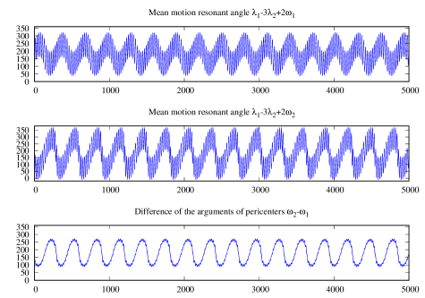
Figure 1: Evolutions in time (whose adopted unit of measure is year) of the libration angles, which are measured in degrees and their corresponding plots of $\lambda_{1}-3\lambda_{2}+2\omega_{1}\,$, $\lambda_{1}-3\lambda_{2}+2\omega_{2}$ and $\omega_{2}-\omega_{1}$ appear in the panels above from top to bottom, respectively.

For what concerns the eccentricities, looking at Fig. 2 one can easily remark that the one of the inner planet can also exceed the value $0.3$, during its dynamical evolution. This makes evident that the orbital configuration of these exoplanets is quite different with respect to that of the biggest planets of our Solar System, whose orbits are nearly circular. Therefore, it is natural to expect that a remarkable effort will be needed to adapt normal forms algorithms which worked efficiently to construct quasi-periodic approximations of the orbital motions of the major planets in our Solar System (see [26] and [27]). In order to efficiently implement a normal form approach to the HD60532 extra-solar system, we will need to design a few modifications to that basic scheme. This has to be done in such a way to make it more similar to the approach that successfully worked in the case of the $\upsilon$ Andromedæ planetary system (see [5]), which also shows the phenomenon of the librations of the difference of the pericenters arguments (i.e., the so called apsidal locking) as in the case under study of HD60532.

Figure 2: Evolutions in time (measured in years) of the semi-major axes [AU] and eccentricities of the exoplanets hosted in the HD60532 extra-solar system.

3.1 The resonant model

Being interested in the long-term dynamics of a system that is in MMR, we consider a resonant approximation of the Hamiltonian that allows to reduce the number of degrees of freedom to 2. Hence, we now consider a set of coordinates which allows to better highlight this point. First of all, let us introduce the action-angle variables $(\bm{I},\bm{\omega})$ which replace the secular variables $(\bm{\xi},\bm{\eta})$ by means of the following canonical transformation:

$$\xi_{j}=\sqrt{2I_{j}}\cos(\omega_{j})\ ,\qquad\eta_{j}=-\sqrt{2I_{j}}\sin(\omega_{j})\ ,\qquad\text{for}\quad j=1,2\ .$$

Now, we also introduce the resonant variables related to the two libration angles,

$$\left\{\begin{aligned} &p_{\delta}=I_{1}+2L_{1}\\ &p_{\sigma}=L_{1}\\ &p_{\phi}=I_{1}+I_{2}+2L_{1}\\ &p_{\theta}=L_{2}+3L_{1}\end{aligned}\right.\qquad\qquad\left\{\begin{aligned} &\delta=\omega_{2}-\omega_{1}\\ &\sigma=\lambda_{1}-3\lambda_{2}+2\omega_{1}\\ &\phi=-\omega_{2}\\ &\theta=\lambda_{2}\end{aligned}\right.\quad.$$

In this new set of action-angle coordinates, we consider the average of the Hamiltonian over the (unique) non-resonant revolution angle $\theta$, i.e.,

$$\bar{H}=\frac{1}{2\pi}\int_{0}^{2\pi}H\big{(}p_{\delta}\,,\,p_{\sigma}\,,\,p_{\phi}\,,\,p_{\theta}\,,\,\delta\,,\,\sigma\,,\,\phi\,,\,\theta\big{)}\,{\rm d}\theta\ .$$

Therefore, the angles $\phi$ and $\theta$ turn out to be cyclic variables for the Hamiltonian $\bar{H}$. Indeed, the action $p_{\phi}$ is exactly the total angular momentum, which is a constant of motion for the whole three-body planetary system. Since we perform an average of the Hamiltonian with respect to a fast angle of orbital revolution, then it is usual to refer to $\bar{H}$ as a resonant approximation at order one in the masses. Such an averaged model shows two first integrals and can be reduced to two degrees of freedom. The accuracy of the approximation at order one in the masses is discussed in [22] and [33], for general $2$D three-body models of exoplanetary systems and for particular cases in mean-motion resonance, respectively. This is made by means of comparisons with the results provided by both the approximation at order two in the masses and the numerical integrations of the non-averaged system.

The center of the librations of the resonant angles $\delta$ and $\sigma$ corresponds to an equilibrium point of the angle variables of the resonant Hamiltonian $\bar{H}$. With the aim of expanding the Hamiltonian $\bar{H}$ around its equilibrium point, we also look for the values, say $(p_{\delta}^{*},p_{\sigma}^{*})$, of the conjugate momenta $p_{\delta}$ and $p_{\sigma}$ such that the Jacobian of the Hamiltonian $\bar{H}$ is equal zero. Once we have determined the equilibrium point $(p_{\delta}^{*},p_{\sigma}^{*},\pi,\pi)$, we can translate the origin of the canonical variables, by defining

$$y_{1}=p_{\delta}-p_{\delta}^{*}\ ,\quad y_{2}=p_{\sigma}-p_{\sigma}^{*}\ ,\quad x_{1}=\delta-\pi\ ,\quad x_{2}=\sigma-\pi\ ,$$

and expand the Hamiltonian in Taylor series around the origin. We also proceed with a diagonalization of the quadratic part of the Hamiltonian. Indeed, there is a linear canonical transformation $(y_{1},y_{2},x_{1},x_{2})=\mathcal{C}(Y_{1},Y_{2},X_{1},X_{2})$ conjugating the quadratic approximation to a couple of harmonic oscillators. As a result, the Hamiltonian in the new polynomial variables $(\bm{Y},\bm{X})$ reads

$$H(\bm{Y},\bm{X})=\frac{\omega_{1}}{2}(Y_{1}^{2}+X_{1}^{2})+\frac{\omega_{2}}{2}(Y_{2}^{2}+X_{2}^{2})+\sum_{\ell\geq 1}h_{\ell}(\bm{Y},\bm{X})\ ,$$ (1)

where the functions $h_{\ell}$ are homogeneous polynomials of degree $\ell+2$ in the variables $(\bm{Y},\bm{X})$. Let us remark that, according to a standard notation in the context of the KAM theory, hereafter, $\omega_{1}$ and $\omega_{2}$ are used to denote the frequencies (while they have been used before to refer to the arguments of the pericenters).

The main goal of this work is to investigate the stability of the Hamiltonian model given by (1) and to reconstruct its quasi-periodic motion, starting from initial conditions corresponding to the data reported in Table 1. First of all, let us stress that the Hamiltonian (1) has an elliptic equilibrium point at the origin and, in addition, in the case of the extra-solar system HD60532, the two frequencies $\omega_{1}$ and $\omega_{2}$ also have the same sign. Hence, it would be quite natural to try to deal with the problem using a Lyapunov confinement argument about the values of the actions after having performed a few steps of the Birkhoff normalization algorithm. However, this approach fails because the initial conditions (expressed in the polynomial variables $(\bm{Y},\bm{X})$) are too far from the equilibrium point situated at the origin. Hence, we need a less naif method in order to tackle the problem under study. Therefore, one could try another constructive procedure that has shown to be successful in a similar context, i.e., for models of the secular planetary dynamics (see [25], [13] and [36]). Indeed, it could be convenient to first introduce action-angle variables, with the aim of performing a translation of the actions and then applying the standard Kolmogorov normalization algorithm. Nevertheless, also this attempt fails, because it is not enough to achieve the convergence of the final procedure, even if preceded by a finite number of steps of the Birkhoff normalization algorithm.

We are then led to develop a different approach which is adapted to the special kind of problem we are considering. Let us remark that in this model a slow dynamics can be distinguished from a faster one, as we can see from the plots of the two libration angles that are reported in the first panel of Fig. 1 and the third one. In particular, the difference of the argument of the pericenters points out the slow period, that is $\mathcal{O}(1/\mu)$, while the mean motion resonant angle $\sigma$ also highlights the presence of a faster period. Therefore, the key strategy to face the problem is to preliminarly average the Hamiltonian with respect to the faster libration angle, namely over an angle related to the MMR. Let us recall that, by applying the procedure mentioned in footnote${\ref{nota:diagonalization}}\atop{\phantom{1}}$, it can be easily shown that the period of such a (so called) fast libration angle is $\mathcal{O}(1/\sqrt{\mu})$. Therefore, it is somehow intermediate between the secular angles and the orbital revolution ones. This justifies the name we have decided to adopt, in order to refer to it.

4 Average over the fast libration angle

In this section we describe the algorithm which allows to perform the average of the Hamiltonian with respect to the fast libration angle.

We introduce the action-angle variables $(\bm{J},\bm{\vartheta})$ via the canonical transformation $(\bm{Y},\bm{X})=\mathcal{A}(\bm{J},\bm{\vartheta})$, namely

$$Y_{j}=\sqrt{2J_{j}}\cos(\vartheta_{j})\ ,\qquad X_{j}=\sqrt{2J_{j}}\sin(\vartheta_{j})\ ,\qquad\text{for}\quad j=1,2\ .$$ (2)

After this canonical change of coordinates the Hamiltonian (1) reads

$$\mathcal{H}^{(0)}(\bm{J},\bm{\vartheta})=\bm{\omega}\cdot\bm{J}+\sum_{\ell\geq 1}h^{(0)}_{\ell}(\bm{J},\bm{\vartheta})\ ,\qquad\text{with}\quad(\bm{J},\bm{\vartheta})\in{\mathbb{R}}^{2}\times\mathbb{T}^{2}\ ,$$ (3)

where the functions $h^{(0)}_{\ell}$ are homogeneous polynomials of degree $\ell+2$ in the square root of the actions $\bm{J}$ and trigonometric polynomials in the angles $\bm{\vartheta}$. The superscript refers to the normalization step of the averaging algorithm we are going to describe in detail.

4.1 Formal algorithm for the construction of a resonant Birkhoff normal form

As usual, this normal form is constructed by using the Lie series formalism, with the Lie series operator $\exp\left(\mathcal{L}_{\chi}\right)$ defined as follows:

$$\exp\left(\mathcal{L}_{\chi}\right)=\displaystyle\sum_{s\geq 0}\dfrac{1}{s!}\mathcal{L}_{\chi}^{s}\quad\text{and}\quad\mathcal{L}_{\chi}\cdot=\left\{\cdot,\chi\right\}\ .$$

Moreover, we denote by $\mathcal{P}_{s}$ the class of functions depending on the action-angle variables $(\bm{J},\bm{\vartheta})$ in such a way that, $\forall\ g\in\mathcal{P}_{s}$, $g\circ\mathcal{A}^{-1}$ is an homogeneous polynomial of degree $s$ in the cartesian canonical variables $(\bm{Y},\bm{X})$. In more detail, the Taylor-Fourier expansion of a generic function $g\in\mathcal{P}_{s}$ can be written as

$$g(\bm{J},\bm{\vartheta})=\!\!\!\sum_{\scriptstyle{{\bm{\ell}\in\mathbb{N}^{2}}\atop{\ell_{1}+\ell_{2}=s}}}\!\!\,\sum_{\scriptstyle{{k_{1}=-\ell_{1},\,-\ell_{1}+2,\ldots,\,\ell_{1}}\atop{k_{2}=-\ell_{2},\,-\ell_{2}+2,\ldots,\,\ell_{2}}}}\!\!\!\!\!\!\!\!c_{\bm{\ell},\bm{k}}\,\big{(}\sqrt{J_{1}}\big{)}^{\ell_{1}}\,\big{(}\sqrt{J_{2}}\big{)}^{\ell_{2}}\exp\big{[}{\rm i}(k_{1}\vartheta_{1}+k_{2}\vartheta_{2})\big{]}\>,$$ (4)

where the complex coefficients are such that $c_{\bm{\ell},-\bm{k}}={\bar{c}}_{\bm{\ell},\bm{k}}$. For the sake of brevity, in the following we will adopt the usual multi-index notation for the powers in the square roots of the actions, i.e, the product $(\sqrt{J_{1}})^{\ell_{1}}\,(\sqrt{J_{2}})^{\ell_{2}}$ will be denoted as $(\sqrt{\bm{J}})^{\bm{\ell}}$; moreover, they will be subject to the restriction $|\bm{\ell}|=s$ for every term appearing in the expansion of a function $g\in\mathcal{P}_{s}\,$, being $|\bm{\ell}|:=\ell_{1}+\ell_{2}\,$. In the following Lemma, we are going to describe the behaviour of such a class of functions with respect to the Poisson brackets.

Lemma 4.1

Let $f\in\mathcal{P}_{s_{1}+2}$ and $g\in\mathcal{P}_{s_{2}+2}\,$, then $\{f,g\}\in\mathcal{P}_{s_{1}+s_{2}+2}$ $\forall\ s_{1}\in\mathbb{N}\setminus\{0\}\,$, $s_{2}\in\mathbb{N}\setminus\{0\}$.

Proceeding in a perturbative way, we want to remove step by step the dependence on the fast angle $\vartheta_{2}$ (which is related to the fast libration angle $\sigma$) from the perturbative part of the Hamiltonian. Hence, after having performed $r-1$ canonical changes of coordinates defined by the Lie series operator, the Hamiltonian (3) is brought to the following form:

$$\mathcal{H}^{(r-1)}(\bm{J},\bm{\vartheta})=\bm{\omega}\cdot\bm{J}+\sum_{\ell=1}^{r-1}Z_{\ell}(\bm{J},\vartheta_{1})+\sum_{\ell\geq r}h_{\ell}^{(r-1)}(\bm{J},\bm{\vartheta})\ ,$$

where $Z_{\ell}\in\mathcal{P}_{\ell+2}$ and $h_{\ell}^{(r-1)}\in\mathcal{P}_{\ell+2}\,$.

Let us remark that, with abuse of notation, we are denoting the new action-angle variables (that are introduced by the canonical transformation defined by any normalization step) with the same pair of symbols $(\bm{J},\bm{\vartheta})$, which has been used to denote the arguments of $\mathcal{H}^{(0)}$. As it is usual for the Lie series formalism, this is done in order to contain the proliferation of the symbols.

The Hamiltonian in normal form up to order $r$ is obtained as $\mathcal{H}^{(r)}=\exp\left(\mathcal{L}_{\chi_{r}}\right)\mathcal{H}^{(r-1)}$, where the generating function $\chi_{r}$ is determined by solving the homological equation

$$\mathcal{L}_{\chi_{r}}\left(\bm{\omega}\cdot\bm{J}\right)+h_{r}^{(r-1)}(\bm{J},\bm{\vartheta})=Z_{r}(\bm{J},\vartheta_{1})\ ,$$

with $Z_{r}(\bm{J},\vartheta_{1}):=\langle h^{(r-1)}_{r}\rangle_{\vartheta_{2}}$ where as usual $\langle\cdot\rangle_{\psi}$ denotes the angular average with respect to $\psi$. In order to solve such an equation, let us first write the Taylor-Fourier expansion of the perturbative term as

$$h_{r}^{(r-1)}(\bm{J},\bm{\vartheta})=\sum_{\scriptstyle{{\bm{\ell}\in\mathbb{N}^{2}}\atop{|\bm{\ell}|=r+2}}}\,\sum_{\scriptstyle{{k_{1}=-\ell_{1},\,-\ell_{1}+2,\ldots,\,\ell_{1}}\atop{k_{2}=-\ell_{2},\,-\ell_{2}+2,\ldots,\,\ell_{2}}}}c_{\bm{\ell},\bm{k}}^{(r)}\,\big{(}\sqrt{\bm{J}}\big{)}^{\bm{\ell}}\exp\big{(}{\rm i}\bm{k}\cdot\bm{\vartheta}\big{)}\ .$$

Therefore, the $r$-th generating function writes as

$$\chi_{r}(\bm{J},\bm{\vartheta})=\sum_{\scriptstyle{{\bm{\ell}\in\mathbb{N}^{2}}\atop{|\bm{\ell}|=r+2}}}\,\sum_{\scriptstyle{{k_{1}=-\ell_{1},\,-\ell_{1}+2,\ldots,\,\ell_{1}}\atop{k_{2}=-\ell_{2},\,-\ell_{2}+2,\ldots,\,\ell_{2}\,;\ k_{2}\neq 0}}}\frac{c_{\bm{\ell},\bm{k}}^{(r)}}{{\rm i}\bm{k}\cdot\bm{\omega}}\,\big{(}\sqrt{\bm{J}}\big{)}^{\bm{\ell}}\exp\big{(}{\rm i}\bm{k}\cdot\bm{\vartheta}\big{)}\ .$$

Clearly, the generating function can be properly defined if and only if the frequency vector $\bm{\omega}$ is non-resonant up to the order $r+2$. This means that $\bm{k}\cdot\bm{\omega}\neq 0$ $\forall\ 0<|\bm{k}|\leq r+2$. Such a property is certainly satisfied if we assume that $\bm{\omega}$ satisfies the Diophantine condition, namely

$$|\bm{k}\cdot\bm{\omega}|\geq\frac{\gamma}{|\bm{k}|^{\tau}}\ ,\quad\forall\ \bm{k}\in{\mathbb{R}}^{2}\setminus\{0\}\ ,$$

for some fixed values of $\gamma>0$ and $\tau\geq 1$. Let us also recall that almost all the vectors in ${\mathbb{R}}^{2}$ are Diophantine with respect to the Lebesgue measure.

The transformed functions $h_{\ell}^{(r)}$ appearing in the expansion of the new Hamiltonian

$$\mathcal{H}^{(r)}(\bm{J},\bm{\vartheta}) =\mathcal{Z}^{(r)}(\bm{J},\vartheta_{1})+\mathcal{R}^{(r+1)}(\bm{J},\bm{\vartheta})$$ (5)

$$=\bm{\omega}\cdot\bm{J}+\sum_{\ell=1}^{r}Z_{\ell}(\bm{J},\vartheta_{1})+\sum_{\ell\geq r+1}h_{\ell}^{(r)}(\bm{J},\bm{\vartheta})\ ,$$

are defined as follows

$$h_{\ell}^{(r)}=\sum_{j=0}^{\lfloor\ell/r\rfloor}\frac{1}{j!}\mathcal{L}_{\chi_{r}}^{j}h^{(r-1)}_{\ell-jr}\ ,\qquad\qquad\hbox{for }{\vtop{\hbox{$\ \ell\geq r+1$\ .} }}$$

A simple induction argument, which is based on the application of Lemma 4.1, allows us to verify that $h^{(r)}_{\ell}\in\mathcal{P}_{\ell+2}$ $\forall\ \ell$. Hence, after a finite number $r$ of normalization steps, we get the Hamiltonian $\mathcal{H}^{(r)}$, which is the sum of a normal form part $\mathcal{Z}^{(r)}(\bm{J},\vartheta_{1})=\bm{\omega}\cdot\bm{J}+\sum_{\ell=1}^{r}Z_{\ell}(\bm{J},\vartheta_{1})$, which is integrable, and a remainder $\mathcal{R}^{(r+1)}(\bm{J},\bm{\vartheta})=\sum_{\ell\geq r+1}h_{\ell}^{(r)}(\bm{J},\bm{\vartheta})$. Indeed, the averaged part $\mathcal{Z}^{(r)}(\bm{J},\vartheta_{1})$ is independent of the fast angle $\vartheta_{2}$. Therefore, the action $J_{2}$ is constant along the flow induced by $\mathcal{Z}^{(r)}$, because $\big{\{}J_{2}\,,\,\mathcal{Z}^{(r)}\big{\}}=0\,$. Moreover, the averaged part $\mathcal{Z}^{(r)}$ results in an integrable approximation, because it can be reduced to an Hamiltonian having just one degree of freedom.

For later convenience, it is also worth to recall that the canonical transformation $\mathcal{C}^{(r)}$ defining the resonant Birkhoff normal form up to the $r$-th step of the constructive algorithm is explicitly given by

$$\mathcal{C}^{(r)}(\bm{J},\bm{\vartheta})=\exp\mathcal{L}_{\chi_{r}}\,\circ\,\exp\mathcal{L}_{\chi_{r-1}}\,\circ\,\ldots\,\exp\mathcal{L}_{\chi_{1}}\,(\bm{J},\bm{\vartheta})\ .$$ (6)

In fact, the exchange theorem for Lie series ensures us that $\mathcal{H}^{(r)}(\bm{J},\bm{\vartheta})=\mathcal{H}^{(0)}\big{(}\mathcal{C}^{(r)}(\bm{J},\bm{\vartheta})\big{)}$ $\forall\ (\bm{J},\bm{\vartheta})\in\mathcal{B}(\bm{0})\times\mathbb{T}^{2}$, being $\mathcal{B}(\bm{0})$ a suitable open ball centered around the origin of ${\mathbb{R}}^{2}$ (see [15] and [10]).

4.2 Comparison between numerical integrations and semi-analytic solutions

In this subsection, we are going to check the validity of the averaged Hamiltonian up to a finite order $\tilde{r}$ (namely the integrable approximation $\mathcal{Z}^{(\tilde{r})}$) in describing the orbital motions induced by the Hamiltonian (1) which describes the slow dynamics of a planetary system in MMR. For what concerns our extra-solar model, this latter Hamiltonian, expressed in action-angle variables as in (3), has been expanded up to order $6$ in the square root of the actions. We perform $6$ normalization steps and our goal is to compare numerical integrations of the Hamiltonian in MMR (1) with the semi-analytic solution of the averaged Hamiltonian up to order $6$, both described in the cartesian variables $Y_{j}=\sqrt{2J_{j}}\cos(\vartheta_{j})$ and $X_{j}=\sqrt{2J_{j}}\sin(\vartheta_{j})$, for $j=1,2$. The choice $\tilde{r}=6$ allows to obtain a reasonable balance between the accuracy and the needed computational time.

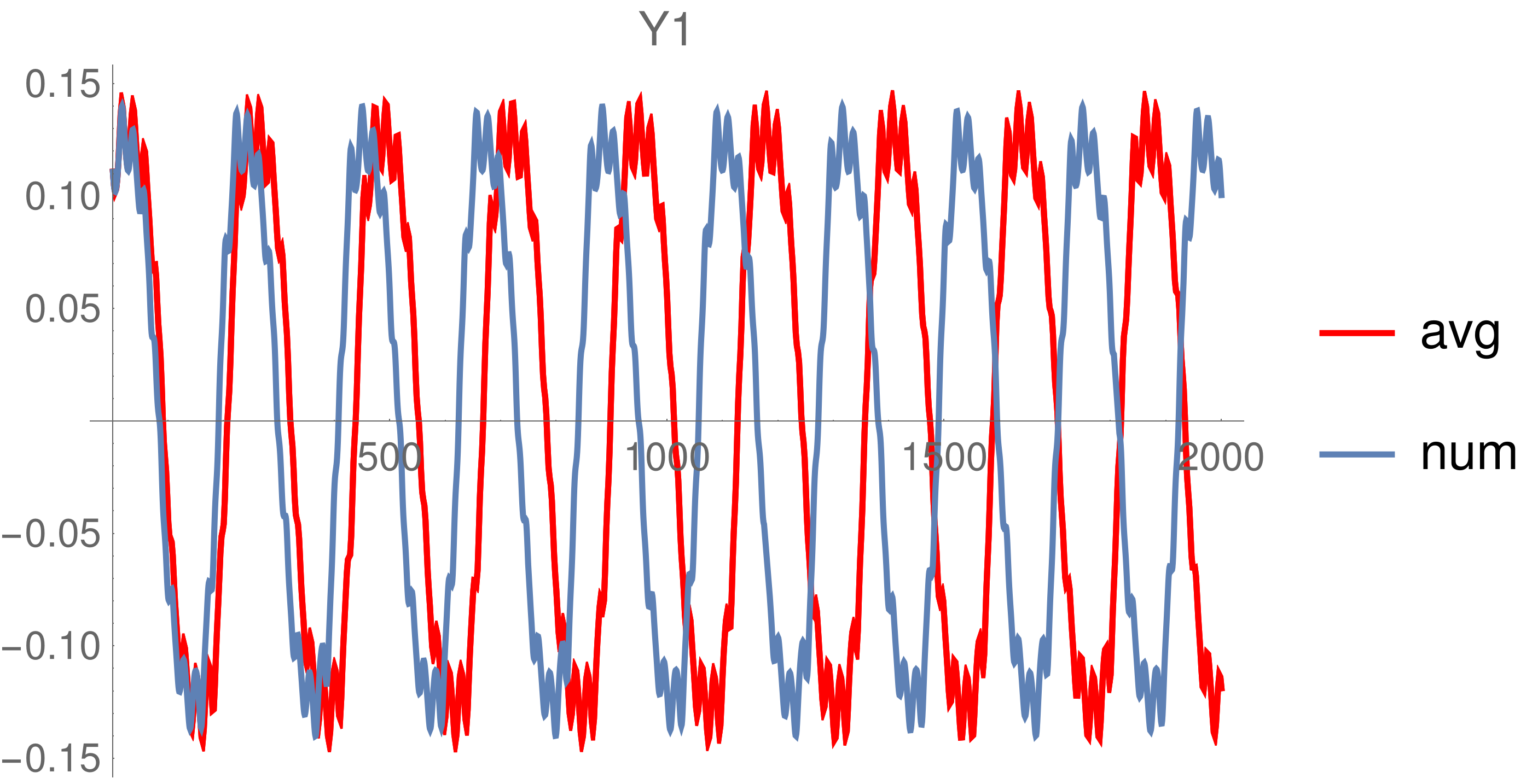
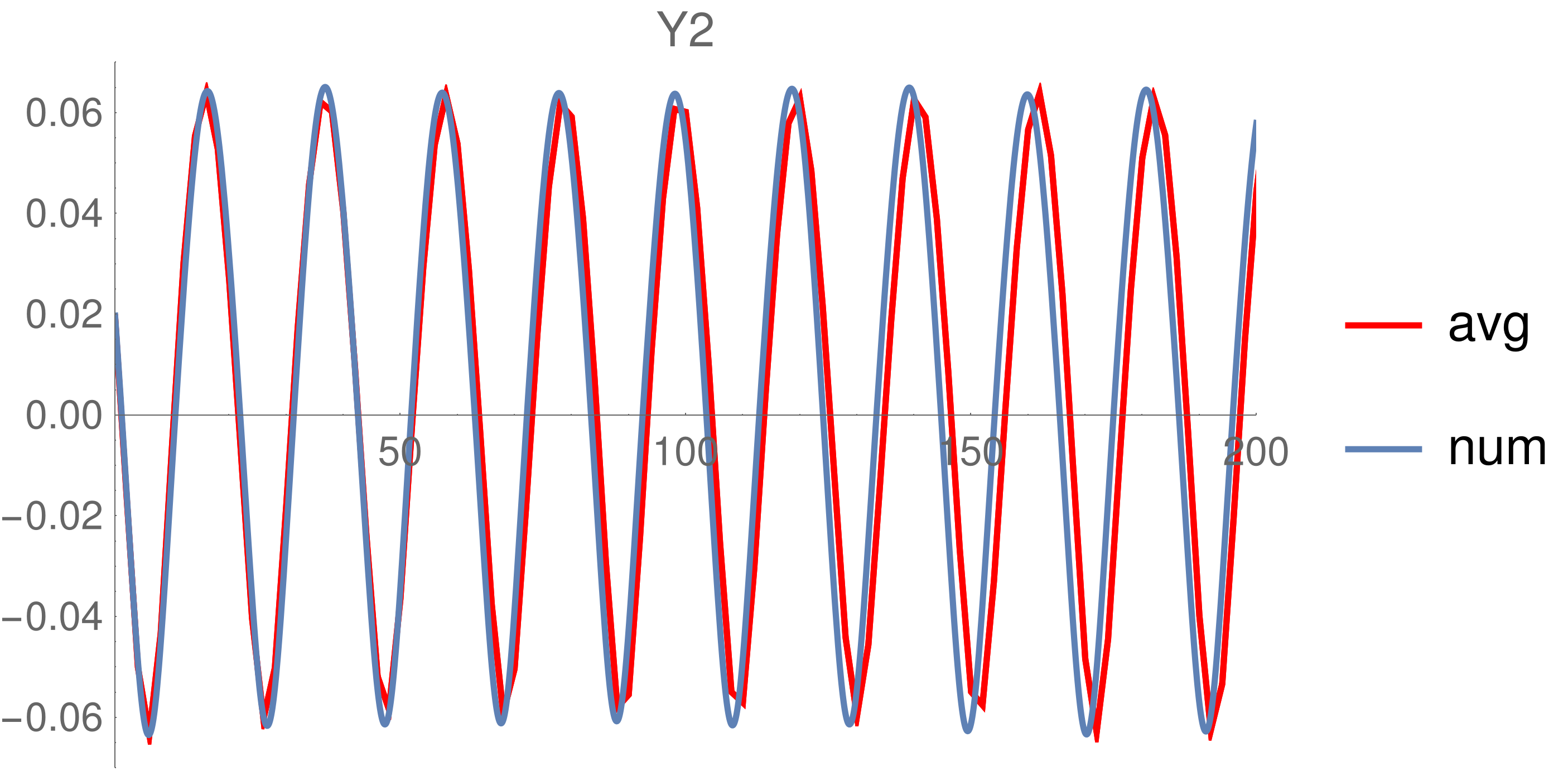
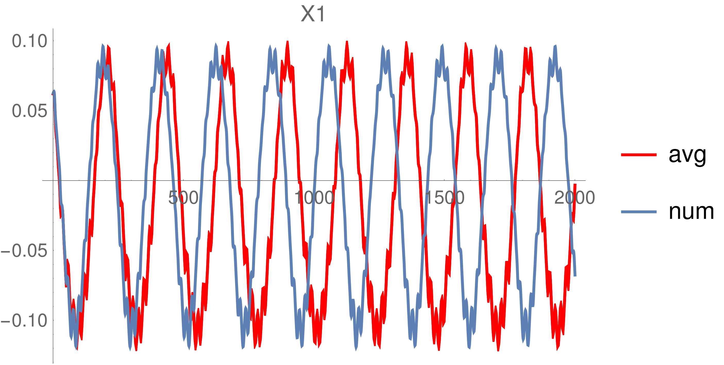
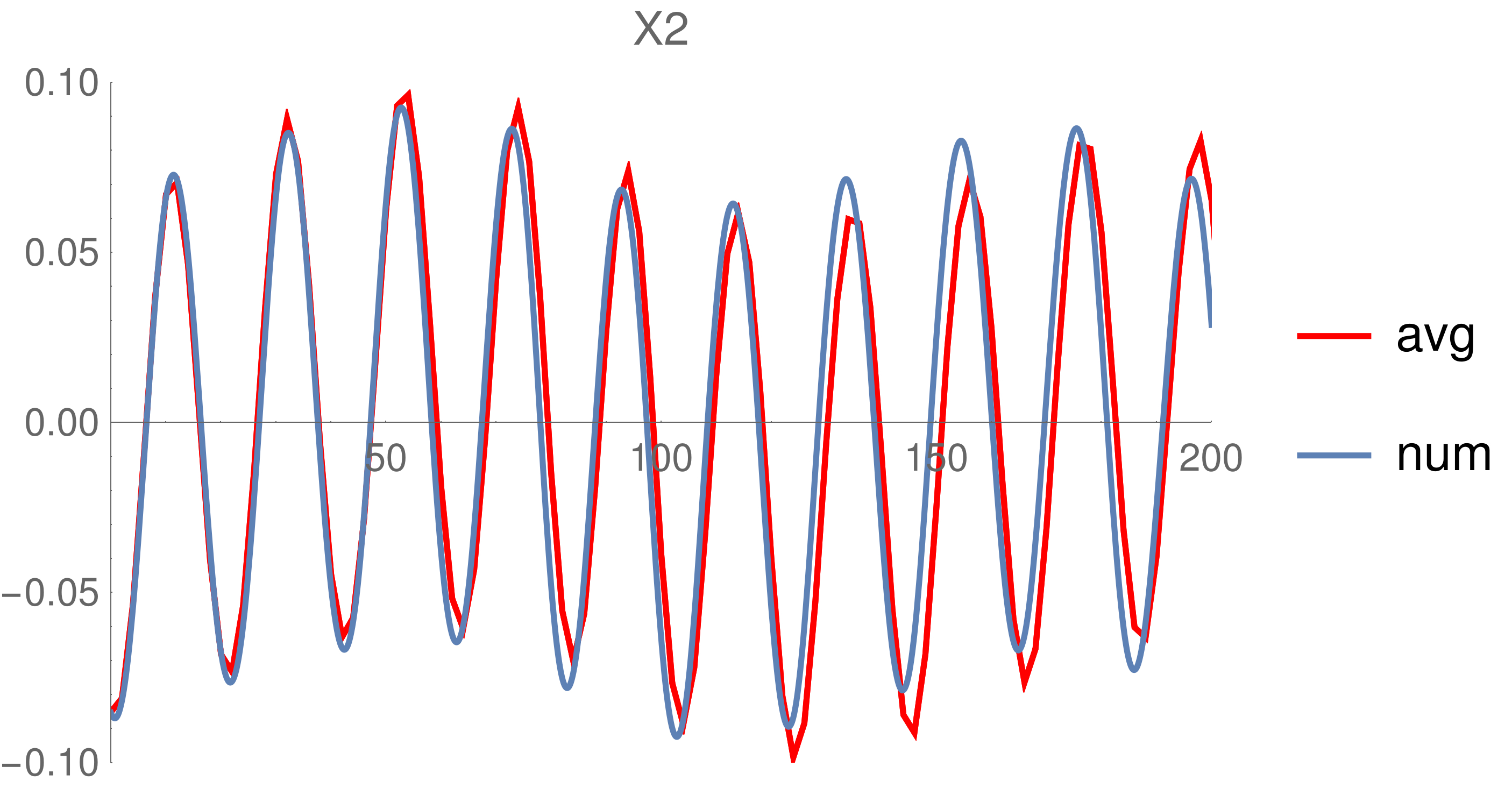
Figure 3: Evolutions in time [yr] of the slow variables (left panels) and the fast ones (right panels), given by the numerical integrations of the Hamiltonian (1) (blue curves) and the semi-analytic solution of the averaged Hamiltonian $\mathcal{Z}^{(6)}$ (red curves).

Let us recall that the averaged Hamiltonian $\mathcal{Z}^{(6)}$ is integrable according to the Liouville-Arnold-Jost theorem (for a complete proof, see, e.g., [10]). Therefore, there exists an analytic expression (eventually involving also the computation of integrals and the inversion of some functions) which defines a canonical transformation $(\bm{J},\bm{\vartheta})=\Psi(\bm{P},\bm{\varphi})$, such that the averaged approximation $\mathcal{Z}^{(6)}$ depends on the actions $\bm{P}$ only, when it is transformed according to the change of variables $\Psi$, i.e.,

$$\frac{\partial\,\mathcal{Z}^{(6)}\big{(}\Psi(\bm{P},\bm{\varphi})\big{)}}{\partial\varphi_{j}}=0\quad\forall\ j=1,\,2\ .$$

Thus, in the new set of action-angle variables $(\bm{P},\bm{\varphi})$ the equations of motion related to the averaged Hamiltonian $\mathcal{Z}^{(6)}\circ\Psi$ can be solved very easily. Moreover, we can also evaluate the composition $\mathcal{C}^{(6)}$ of canonical transformations introduced in the previous Subsection in order to define the action-angle variables $(\bm{P},\bm{\varphi})$ and to obtain the Hamiltonian in normal form up to order $6$. The normal form algorithm can be finally translated in a so called semi-analytic procedure which allows to determine the motion law $t\mapsto(\bm{Y}(t),\bm{X}(t))$ that is defined by the flow induced by the averaged Hamiltonian $\mathcal{Z}^{(6)}$. Such a computational procedure is summarized ($\forall\ t\in{\mathbb{R}}$) by the following scheme:

(7)

where $\Phi_{\mathcal{Z}^{(6)}\circ\Psi}^{t}$ is nothing but the flow at time $t$ induced by the Hamiltonian $\mathcal{Z}^{(6)}\circ\Psi$ and the angular velocity is given by $\beta_{j}=\frac{\partial}{\partial P_{j}}\big{(}\mathcal{Z}^{(6)}\circ\Psi\big{)}$, while $\mathcal{A}$ and $\mathcal{C}^{(6)}$ are defined in (2) and (6), respectively. Let us stress that the initial conditions $(\bm{P}(0),\bm{\varphi}(0))$ can be obtained by inverting the composition of the canonical transformations previously described, while the initial conditions $(\bm{Y}(0),\bm{X}(0))$ are the ones derived from the observations. This semi-analytic solution could be compared with the one obtained by a direct integration of the Hamiltonian (1). For the sake of simplicity, we do not perform the last canonical transformation $\Psi$, which is essential to properly define the semi-analytic scheme (7), but it would require to perform some operations (e.g., the aforementioned integrals and the inversions of functions) that can be hard to implement in a fully explicit way. We just exploit the uniqueness of the solution of the corresponding Cauchy problem and we approximate it numerically, by directly integrating the equations of motion of the averaged Hamiltonian $\mathcal{Z}^{(6)}$. Afterwards, we use the canonical transformations (2) and (6) to express the solution in the variables $(\bm{Y}(t),\bm{X}(t))$ and we compare it with the numerical integration of the Hamiltonian (1).

As we can see from the plots in Fig. 3, for the relatively faster pair of variables $(Y_{2},X_{2})$ we have a good agreement between the two solutions, both in terms of amplitude and in terms of frequency. Instead, as regards the slow variables $(Y_{1},X_{1})$, there is a remarkable error concerning the frequency. In principle, this discrepancy might be amended with an approximation at order two in the masses (which can be adapted to planetary systems in MMR, as explained in [33]), but this goes beyond the scope of the present paper.

5 Action-angle variables adapted to the integrable approximation

Before showing that KAM theorem applies in the present context, we need another preliminary essential step in order to make the algorithm convergent. Specifically, we have to introduce a set of action-angle variables, that are more suitable to describe the integrable approximation of the Hamiltonian (5) than the pair $(\bm{J},\bm{\vartheta})$ as it is defined after having performed the canonical transformation $\mathcal{C}^{(6)}$. Indeed, the ideal action-angle coordinates would be $(\bm{P},\bm{\varphi})$, the ones we avoided to compute, because of the technical difficulties due to an eventual application of the Liouville-Arnold-Jost theorem. Let us recall that $P_{1}$ and $P_{2}$ would be constant of motion for the integrable approximation $\mathcal{Z}^{(6)}$ and the same holds true also for the action $J_{2}\,$.

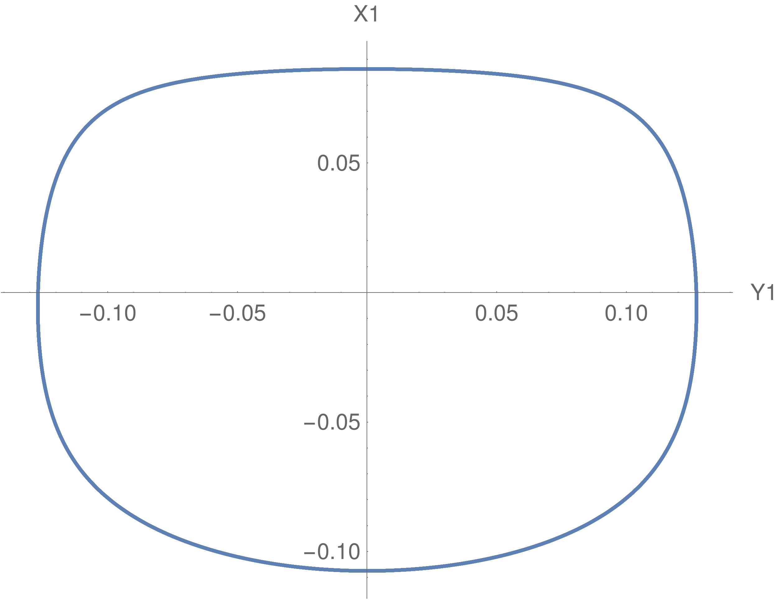
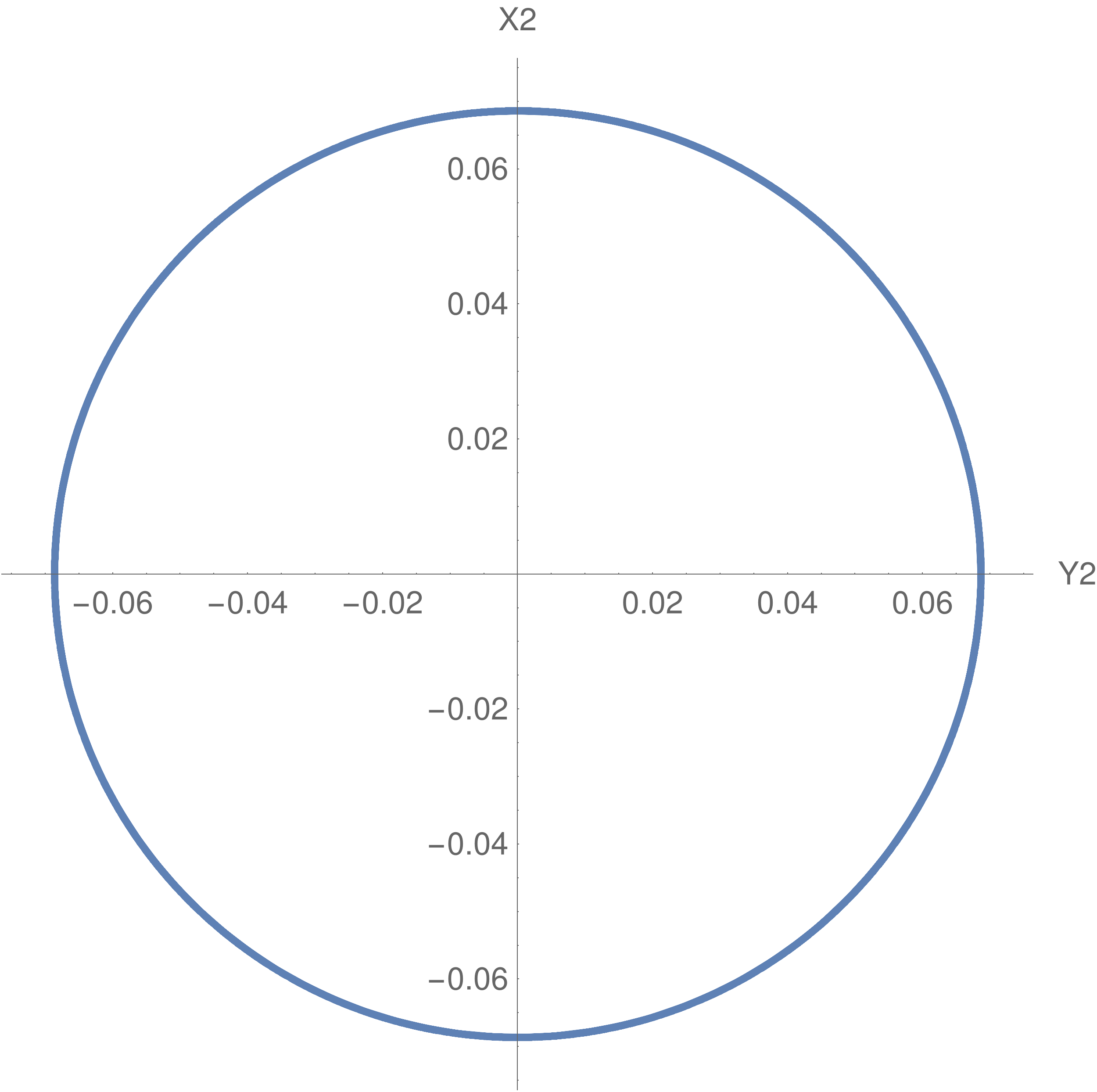
Figure 4: Orbits of the slow dynamics (left panel) and the faster one (right panel) for what concerns the integrable approximation $\mathcal{Z}^{(6)}$. Both the plots refer to the phase space $(\bm{Y},\bm{X})$.

Hence, if we consider the orbit of the fast motion of the integrable approximation $\mathcal{Z}^{(6)}$ in the cartesian variables $(Y_{2},X_{2})=(\sqrt{2J_{2}}\cos(\vartheta_{2}),\sqrt{2J_{2}}\sin(\vartheta_{2}))$, we get a circular orbit, as it is shown in the right panel of Fig. 4. Instead, looking at the orbit of the slow motion in the cartesian variables $(Y_{1},X_{1})=(\sqrt{2J_{1}}\cos(\vartheta_{1}),\sqrt{2J_{1}}\sin(\vartheta_{1}))$, that are related to the secular dynamics, we can observe that such an orbit is far from being circular. Therefore, at this stage we aim at introducing a second action which is closer than $J_{1}$ to be a constant of motion. In other words, our approach consists in the construction of action-angle variables with the aim of trying to circularize (at least partially) the orbit describing the slow dynamics in the integrable approximation. Thus, trying to introduce an action which depends only on the distance from the origin in the cartesian plane endowed with coordinates $(Y_{1},X_{1})$, we are dealing with a quasi-constant of motion and we approach better the sought (final) KAM torus. From a practical point of view, our approach is translated in an explicit computational procedure, by suitably applying the frequency analysis method to the flow induced by the integrable approximation $\mathcal{Z}^{(6)}$ (see [19] for an introduction to such a numerical technique). This can be done by studying the Fourier decomposition of the signal $Y_{1}(t)+{\rm i}X_{1}(t)\simeq\sum_{j=1}^{\mathcal{N}_{c}}A_{1,j}e^{{\rm i}(k_{j}\nu_{1}t+\varphi_{1,j})}$, where $\mathcal{N}_{c}$ is the number of components considered, $A_{1,j}>0$, $k_{j}\in\mathbb{Z}$, $\varphi_{1,j}\in(-\pi,\pi]$ and $2\pi/\nu_{1}$ is the period of such a motion law. By taking into consideration only the $\mathcal{N}_{c}=3$ components of the signal which correspond to $k_{j}=0,\pm 1$ for $j=1,2,3$, it is easy to show that the corresponding approximation of the orbit which describes the secular dynamics is an ellipse. Therefore, in order to give a circular shape to such an approximation of the orbit it is necessary to perform two changes of coordinates: a shift on the variable $X_{1}$ of a translation value $X_{1}^{*}$ and a dilatation/contraction with coefficient $\alpha$. The value $X_{1}^{*}$ of the translation is determined by exploiting the constant component (because for $j=1$ we have $k_{1}=0$ and $\varphi_{1,1}=-\pi/2$, then $A_{1,j}e^{{\rm i}\varphi_{1,1}}$ is purely imaginary and so is aligned with the $X_{1}$ axis), while the coefficient $\alpha$ is defined as follows

$$\alpha=\sqrt{\frac{c_{-}-c_{+}}{c_{-}+c_{+}}}\ ,$$

where $c_{-}$ and $c_{+}$ are the absolute values of the complex coefficients of the components with $k_{2}=-1$ and $k_{3}=1$, respectively. In more detail, we define $c_{-}=A_{1,2}$ and $c_{+}=A_{1,3}$ for $j=2,3$; indeed, the easy computation of the suitable coefficient $\alpha$ of dilatation/contraction takes profit of the values of the corresponding angles, which are such that $\varphi_{1,2}=-\varphi_{1,3}\,$. Therefore, we introduce the new variables

$$v_{1}=\alpha\cdot Y_{1}\ ,\qquad u_{1}=\frac{X_{1}-X_{1}^{*}}{\alpha}\ .$$ (8)

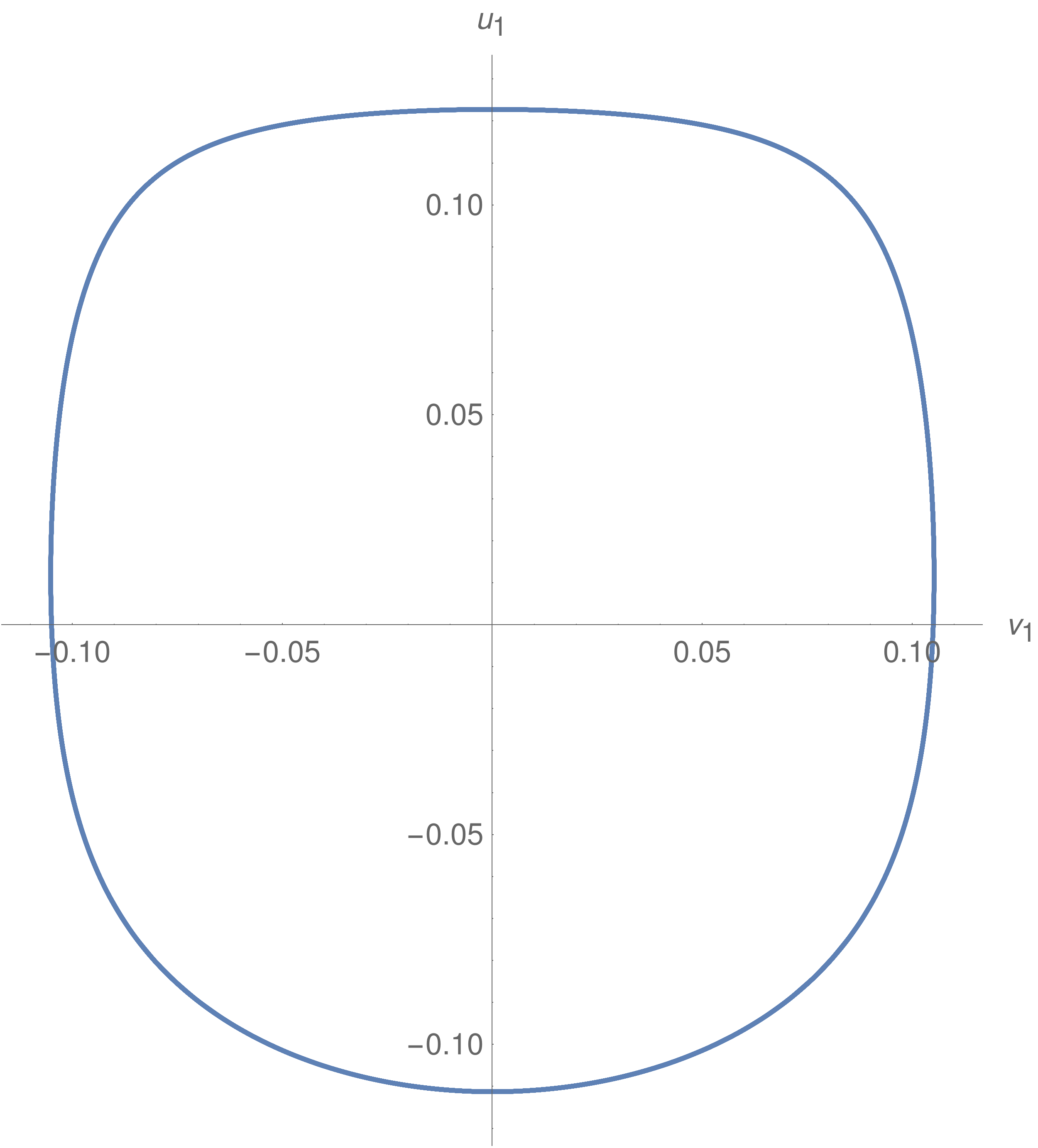
Figure 5: The orbit representing the slow dynamics of the integrable approximation $\mathcal{Z}^{(6)}$ in the phase plane endowed with coordinates $(v_{1},u_{1})$.

The new orbit of the slow motion in the variables $(v_{1},u_{1})$ is represented in Fig. 5. Let us remark that this plot does not represent exactly a circular orbit; this was somehow expected since we have considered only a limited number of Fourier components in the computational method we have introduced in the present Section with the aim of trying to circularize the orbit itself. However, by looking at the scales reported on the vertical axes of the two panels included in Fig. 6, one can appreciate that the canonical change of coordinates (8) allows us to reduce the oscillations of the value of the action involved in the description of the slow dynamics. In fact, when the plot of the motion law $t\mapsto\big{(}Y_{1}^{2}(t)+X_{1}^{2}(t)\big{)}/2$ is compared to the one of $t\mapsto\big{(}v_{1}^{2}(t)+u_{1}^{2}(t)\big{)}/2$, the gain of about 30% in the circularization of the orbit is highlighted. This is enough for the purpose of obtaining a Kolmogorov normalization algorithm which is convergent to the normal form related to the desired final invariant torus.

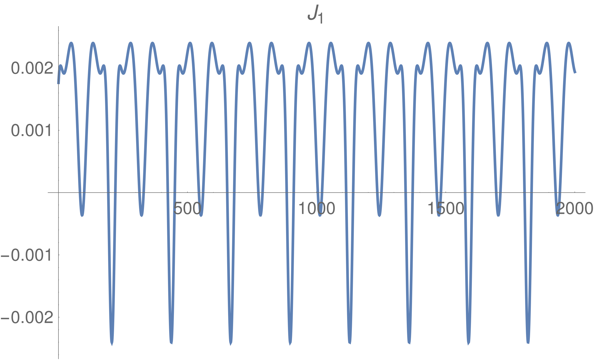
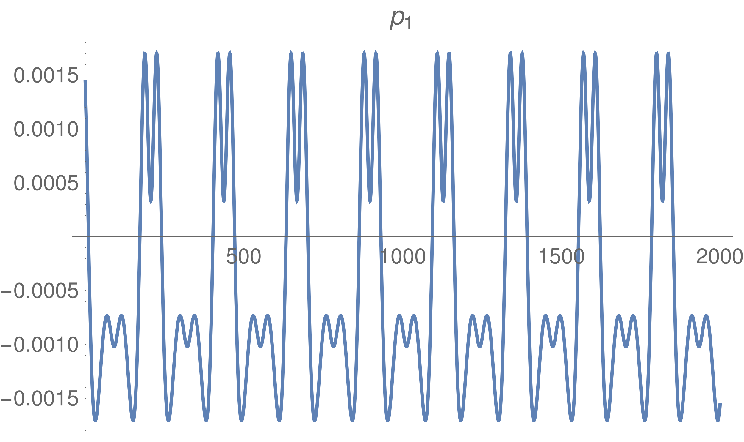
Figure 6: On the left, variation in time of the action $J_{1}=\big{(}Y_{1}^{2}+X_{1}^{2}\big{)}/2$ (with respect to its mid value) along the flow induced by the integrable approximation $\mathcal{Z}^{(6)}$. On the right, the same plot is made for what concerns the action $\big{(}v_{1}^{2}+u_{1}^{2}\big{)}/2$.

We can now introduce the action-angle variables that are more suitably adapted to the integrable approximation, i.e.,

$$v_{1} =\sqrt{2(p_{1}+p_{1}^{*})}\cos(q_{1})\ ,\quad Y_{2} =\sqrt{2J_{2}}\cos(\vartheta_{2})\ ,$$ (9)

$$u_{1} =\sqrt{2(p_{1}+p_{1}^{*})}\sin(q_{1})\ ,\quad X_{2} =\sqrt{2J_{2}}\sin(\vartheta_{2})\ ,$$

where $p_{1}^{*}$ is the value of the area enclosed by the orbit that describes the secular dynamics in the phase plane $(v_{1},u_{1})$ (or in the one endowed with coordinates $(Y_{1},X_{1})$, since canonical transformations preserve the areas) multiplied by the factor $1/(2\pi)$. Therefore, we are imposing that the value $p_{1}^{*}\,$, which corresponds to the closed curve $\big{\{}(p_{1},q_{1})\,:\ p_{1}=0\,,\>q_{1}\in\mathbb{T}\big{\}}$, is equal to the usual definition of the action for Hamiltonian systems with one degree of freedom (see, e.g., Chap. 3 of [10]).

6 Construction of the KAM torus

We can now start the construction of the KAM torus for the averaged dynamics of HD60532. First, we perform a translation of the fast action and we rename the fast angle, i.e.

$$p_{2}=J_{2}-J_{2}^{*}\ ,\qquad q_{2}=\vartheta_{2}\ ,$$ (10)

where $J_{2}^{*}$ is the mean value of the action $J_{2}$. In the new action-angle variables $(\bm{p},\bm{q})$ the Hamiltonian (5) can be expanded as follows

$${H^{(0)}(\bm{p},\bm{q})}$$

(11)

where $f_{\ell}^{(0,s)}$ is a homogeneous polynomial of degree $\ell$ in $\bm{p}$ and a trigonometric polynomial of degree $2s$ in $\bm{q}$. The first superscript of the functions $f_{\ell}^{(0,s)}$ denotes the normalization step. Furthermore, $E^{(0)}$ is the constant of the energy level of $\bm{p}=0$ when $f_{\ell}^{(0,s)}=0$ $\,\forall\ \ell$ and $s=0,\,1$. The goal is to construct the Kolmogorov normal form

$$H^{(\infty)}(\bm{p},\bm{q})=\bm{\omega}^{*}\cdot\bm{p}+\mathcal{O}(\|\bm{p}\|^{2})\ ,$$ (12)

where $\bm{\omega}^{*}$ is the angular velocity vector characterizing the quasi-periodic motion on the invariant (KAM) torus corresponding to $\bm{p}=\bm{0}$. In other words, the Kolmogorov normalization algorithm is designed in such a way to remove the terms appearing in the second row of formula (11) by a sequence of canonical transformations. Here, it is convenient to adopt a different version of the classical Kolmogorov normalization algorithm, which is slightly modified in such a way to not keep fixed the angular velocity vector $\bm{\omega}^{(r)}$, that is defined at the $r$-th step of the procedure and corresponds to the quasi-periodic approximation of the motion on the final sought KAM torus. We basically follow the approach described in [24], where the normalization procedure introduced by Kolmogorov is adapted in such a way to skip the small translation of the actions performed at every step of that algorithm. This modification allows to make the computational procedure more stable; such an improvement can play a crucial role when the action–frequency map is (close to be) degenerate (see [9]). Moreover, in order to improve its efficiency, this small adaptation of the Kolmogorov normalization algorithm has to be formulated so as to suitably determine the preliminary translation in (9). All this computational procedure is summarized in the following in order to make our discussion rather self-consistent.

As in Section 4, it is convenient to introduce suitable classes of functions; here, we are going to say that $g\in{\mathfrak{P}}_{\ell,sK}$ if its Taylor-Fourier expansion writes as

$$g(\bm{p},\bm{q})=\sum_{{\scriptstyle{\bm{j}\in\mathbb{N}^{n}}}\atop{\scriptstyle{|\bm{j}|=\ell}}}\sum_{{\scriptstyle{{\bm{k}\in\mathbb{Z}^{n}}}\atop{\scriptstyle{|\bm{k}|\leq sK}}}}c_{\bm{j},\bm{k}}\,\bm{p}^{\bm{j}}\exp({\rm i}{\bm{k}}\cdot{\bm{q}})\ ,$$ (13)

for some fixed values of the non-negative integer parameters $\ell$, $s$ and $K$. The following statement allows us to describe the behaviour of such a class of functions with respect to the Poisson brackets.

Lemma 6.1

Let us consider two generic functions $g\in{\mathfrak{P}}_{\ell,sK}$ and $h\in{\mathfrak{P}}_{m,rK}\,$, where $K$ is a fixed positive integer number. Then, the following inclusion property holds true:

$$\big{\{}g,h\big{\}}=\mathcal{L}_{h}\,g\in\mathcal{P}_{\ell+m-1,(r+s)K}\quad\ \forall\>\ell,\,m,\,r,\,s\in\mathbb{N}\ {\rm with}\ \ell+m\geq 1\ ,$$

while $\big{\{}g,h\big{\}}=0$ when $\ell=m=0$.

Let us imagine to have already performed $r-1$ normalization steps by using, once again, the Lie series formalism; then, we have to deal with an Hamiltonian of the following type:

$${H^{(r-1)}(\bm{p},\bm{q})}$$

(14)

where $f_{\ell}^{(r-1,s)}\in{\mathfrak{P}}_{\ell,2s}$ $\forall\ \ell,\,s\,\in\mathbb{N}$, while $E^{(r-1)}\in{\mathbb{R}}$. Let us remark that the expansion of $H^{(0)}$, which is reported in (11), agrees with the more general one, that is written just above in (14), in the case with $r=1$. The Kolmogorov normalization algorithm at step $r$ is aimed to remove the main perturbing terms (that are the functions $f_{0}^{(r-1,r)}$ and $f_{1}^{(r-1,r)}$), which are independent of and linear in the actions, respectively.

In order to perform the $r$-th normalization step, first we need to determine the generating function $\chi_{0}^{(r)}$ in such a way to solve the following homological equation:

$$\mathcal{L}_{\chi_{0}^{(r)}}\left(\bm{\omega}^{(r-1)}\cdot\bm{p}\right)+f_{0}^{(r-1,r)}=\langle f_{0}^{(r-1,r)}\rangle_{\bm{q}}\ .$$

As a matter of fact, $\langle f_{0}^{(r-1,r)}\rangle_{\bm{q}}\in{\mathfrak{P}}_{0,0}$ is nothing but a constant term. Therefore, it can be added to $E^{(r-1)}$, in order to update the energy level, whose new value is denoted with $E^{(r)}$. By considering the Taylor-Fourier expansion of the perturbing term we aim to remove, i.e.,

$$f_{0}^{(r-1,r)}(\bm{q})=\sum_{0<|\bm{k}|\leq 2r}c_{\bm{0},\bm{k}}^{(r-1,r)}\exp({\rm i}\bm{k}\cdot\bm{q})\ ,$$

we obtain the following expression for the generating function:

$$\chi_{0}^{(r)}(\bm{q})=\sum_{0<|\bm{k}|\leq 2r}\frac{c_{\bm{0},\bm{k}}^{(r-1,r)}}{{\rm i}\bm{k}\cdot\bm{\omega}^{(r-1)}}\exp({\rm i}\bm{k}\cdot\bm{q})\ .$$

Let us remark that the homological equation can be solved provided that the following non-resonance condition holds true

$$\bm{k}\cdot\bm{\omega}^{(r-1)}\neq 0\ ,\qquad\forall\,\bm{k}\in\mathbb{Z}^{2}\setminus\{0\}\ ,\quad\text{with}\,\,|\bm{k}|\leq 2r\ .$$ (15)

We then introduce the transformed Hamiltonian $\hat{H}^{(r)}=\exp\left(\mathcal{L}_{\chi_{0}^{(r)}}\right)H^{(r-1)}$, whose expansion

$${{\hat{H}^{(r)}}(\bm{p},\bm{q})}$$

(16)

is such that the new Hamiltonian terms $\hat{f}_{\ell}^{(r,s)}$ are defined so that

$$\hat{f}_{0}^{(r,r)} =0\ ,$$

$$\hat{f}_{\ell}^{(r,s)} =\sum_{j=0}^{\lfloor s/r\rfloor}\frac{1}{j!}\mathcal{L}_{\chi^{(r)}_{0}}^{j}f^{(r-1,s-jr)}_{\ell+j}\ ,\qquad\qquad\hbox{for }{\vtop{\hbox{$\ell=0,\ s\neq r$\ ,} \vskip-2.0pt\hbox{\hskip-14.0ptor $\ell\neq 0\ s\geq 0$ \ .}}}$$

By applying repeatedly Lemma 6.1, one can easily verify that $\hat{f}_{\ell}^{(r,s)}\in{\mathfrak{P}}_{\ell,2s}$ $\forall\ \ell,\,s$.

The second generating function $\chi_{1}^{(r)}$ is determined by solving the following homological equation:

$$\mathcal{L}_{\chi_{1}^{(r)}}\left(\bm{\omega}^{(r-1)}\cdot\bm{p}\right)+\hat{f}_{1}^{(r,r)}=\langle\hat{f}_{1}^{(r,r)}\rangle_{\bm{q}}\ .$$ (17)

The term $\langle\hat{f}_{1}^{(r,r)}\rangle_{\bm{q}}\in{\mathfrak{P}}_{1,0}$. This means that it is not dependent on the angles $\bm{q}$ and is linear in the actions $\bm{p}$; thus, it gives a contribution to the definition of the value of the angular velocity vector $\bm{\omega}^{(r)}$, which in principle should converge to its limit $\bm{\omega}^{*}$ (if the normalization algorithm is convergent) and is defined so that

$$\bm{\omega}^{(r)}\cdot\bm{p}=\bm{\omega}^{(r-1)}\cdot\bm{p}+\langle\hat{f}_{1}^{(r,r)}\rangle_{\bm{q}}\ .$$

By considering the following Taylor-Fourier expansion of the new perturbing term we aim to remove, i.e.

$$\hat{f}_{1}^{(r,r)}(\bm{q})-\langle\hat{f}_{1}^{(r,r)}\rangle_{\bm{q}}=\sum_{|\bm{\ell}|=1}\,\sum_{0<|\bm{k}|\leq 2r}\hat{c}_{\bm{\ell},\bm{k}}^{(r,r)}{\bm{p}}^{\bm{\ell}}\exp({\rm i}\bm{k}\cdot\bm{q})\ ,$$

then we easily determine the new generating function as

$$\chi_{1}^{(r)}(\bm{q})=\sum_{|\bm{\ell}|=1}\,\sum_{0<|\bm{k}|\leq 2r}\frac{\hat{c}_{\bm{\ell},\bm{k}}^{(r,r)}}{{\rm i}\bm{k}\cdot\bm{\omega}^{(r-1)}}{\bm{p}}^{\bm{\ell}}\exp({\rm i}\bm{k}\cdot\bm{q})\ .$$

Once again, the homological equation can be solved provided that the frequencies satisfy the non resonance condition (15). The new Hamiltonian is defined as $H^{(r)}=\exp\left(\mathcal{L}_{\chi_{1}^{(r)}}\right)\hat{H}^{(r-1)}$. Its expansion is completely analogous to the one reported in (14). Moreover, the terms $f_{\ell}^{(r,s)}\in{\mathfrak{P}}_{\ell,2s}$ appearing in the expansion of $H^{(r)}$ are defined in the following way:

$$f_{1}^{(r,r)} =0\ ,$$

$$f_{1}^{(r,ir)} =\frac{i-1}{i!}\mathcal{L}_{\chi^{(r)}_{1}}^{i-1}\hat{f}^{(r,r)}_{1}+\sum_{j=0}^{i-2}\frac{1}{j!}\mathcal{L}_{\chi^{(r)}_{1}}^{j}\hat{f}^{(r,(i-j)r)}_{1}\ ,\qquad\qquad\hbox{for }{\vtop{\hbox{$i\geq 2$\ ,}}}$$

$$f_{\ell}^{(r,s)} =\sum_{j=0}^{\lfloor s/r\rfloor}\frac{1}{j!}\mathcal{L}_{\chi^{(r)}_{1}}^{j}\hat{f}^{(r,s-jr)}_{\ell}\ ,\qquad\qquad\hbox{for }{\vtop{\hbox{$\ell=1,\ s\neq ir$\ ,} \vskip-2.0pt\hbox{\hskip-14.0ptor $\ell\neq 1,\ s\geq 0$ \ ,}}}$$

where we have exploited the second homological equation (17).

From a practical point of view, we can iterate the algorithm only up to a finite number of steps, say, $\overline{r}$. This allows us to determine

$$H^{(\overline{r})}(\bm{p},\bm{q})=E^{(\overline{r})}+\bm{\omega}^{(\overline{r})}\cdot\bm{p}+\sum_{s\geq 0}\sum_{\ell\geq 2}f_{\ell}^{(\overline{r},s)}(\bm{p},\bm{q})+\sum_{s\geq\overline{r}+1}\left(f_{0}^{(\overline{r},s)}(\bm{q})+f_{1}^{(\overline{r},s)}(\bm{p},\bm{q})\right)\ .$$ (18)

Hence, we obtain an approximation of the final invariant torus which is characterized by an angular velocity vector $\bm{\omega}^{(\overline{r})}$. If the value (say) $I_{1}^{*}$ of the initial shift on the first action, which has been preliminarly fixed equal to $p_{1}^{*}$ in formula (9), is accurate enough, then the slow frequency $\omega^{(\overline{r})}_{1}$ is close to the one we are aiming at, which is numerically determined by applying the frequency analysis method, namely $\omega^{(\overline{r})}_{1}\simeq\omega_{1}^{*}$. We then calibrate the initial translation of the first action $I_{1}^{*}=p_{1}^{*}$ by means of a Newton method. The goal is to solve the implicit equation $\omega_{1}(\tilde{I}_{1})=\omega_{1}^{*}$ with respect to the initial shift $\tilde{I}_{1}$. The value $\tilde{I}_{1}$ is iteratively computed using the formula

$$\tilde{I}_{1}^{(n)}=\tilde{I}_{1}^{(n-1)}+\frac{\omega_{1}^{*}-\omega_{1}^{(\overline{r})}\left(\tilde{I}_{1}^{(n-1)}\right)}{\omega_{1}^{\prime}\left(\tilde{I}_{1}^{(n-1)}\right)}\ ,$$

where $\tilde{I}_{1}^{(0)}=I_{1}^{*}$ and the value of the derivative $\omega_{1}^{\prime}\big{(}\tilde{I}_{1}^{(n-1)}\big{)}$ is numerically approximated by using the finite difference method. Let us recall that, after having performed the average with respect to the fast angle of libration as it has been described in the previous section, we are mainly focusing on the study of the secular dynamics. In addition, for what concerns the (relatively) faster frequency $\omega_{2}^{(\overline{r})}/(2\pi)$ we automatically have a good enough approximation of both the frequencies of the averaged Hamiltonian, as it can be appreciated looking at the comparison between the semi-analytic solutions showed in Fig. 8, which will be widely commented in the next subsection.

By supposing to iterate the normalization algorithm ad infinitum, one would get the Hamiltonian (12), which admits the invariant torus $\bm{p}=0$ with frequency $\bm{\omega}^{*}$.

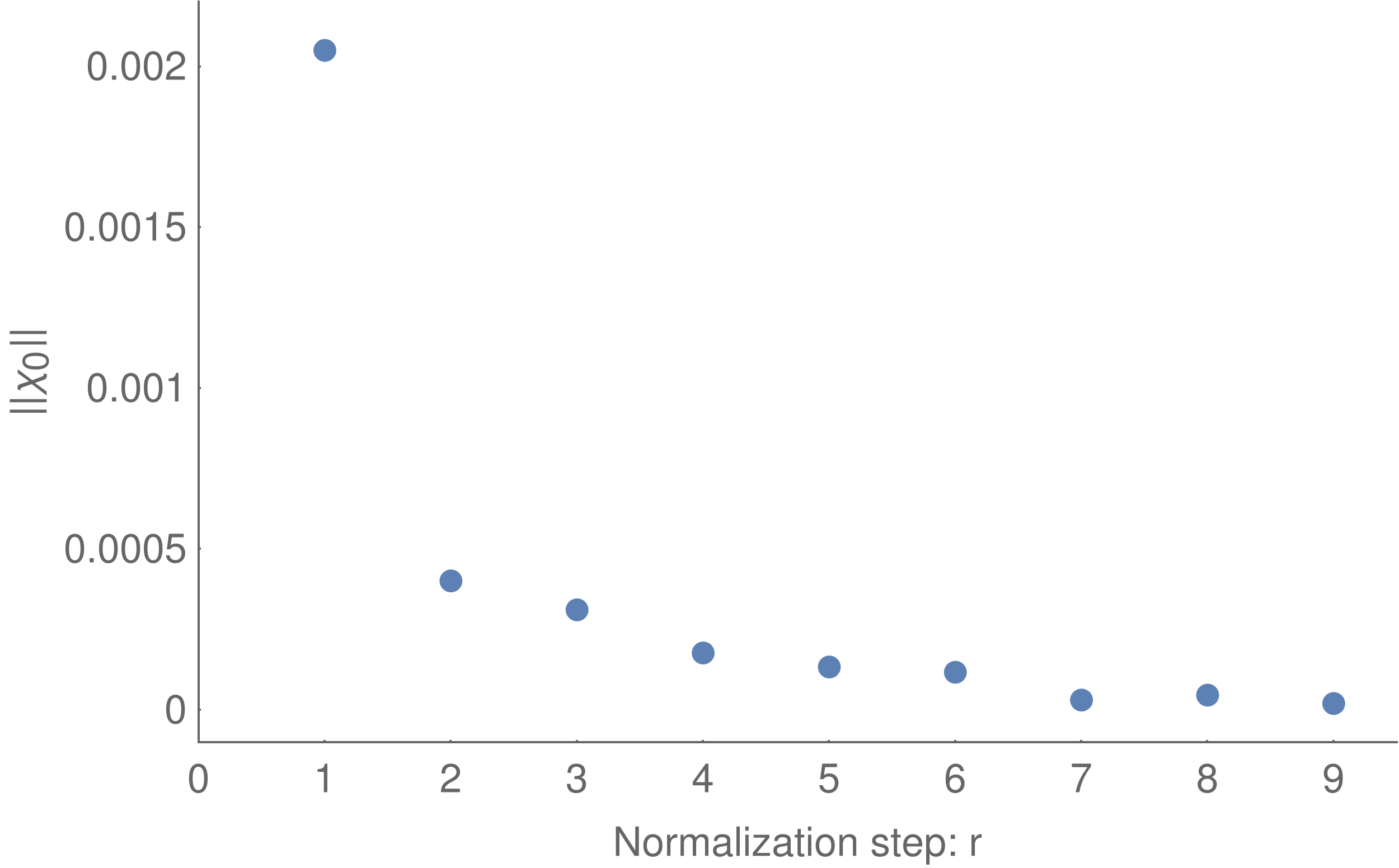
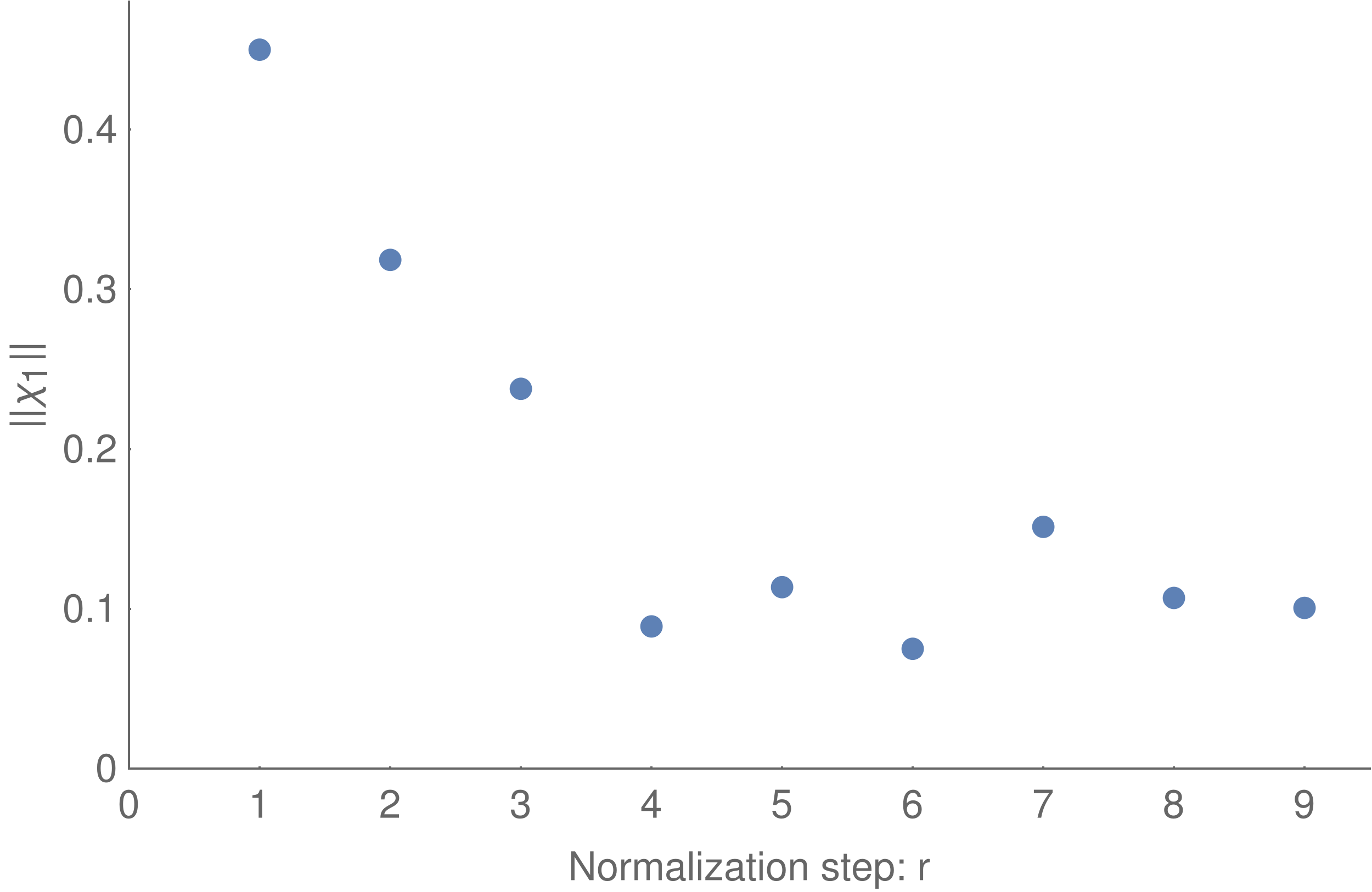
Figure 7: Norms of the generating functions $\chi_{0}^{(r)}$ and $\chi_{1}^{(r)}$ as they are determined by the Kolmogorov algorithm up to the $9$-th normalization step.

From a practical point of view, we are able to explicitly iterate the algorithm only up to a finite normalization step $\overline{r}$ and we can numerically check the convergence of the procedure by controlling the decrease of the norms of the generating functions. Hereafter, we define the norm of any generic function $g\in{\mathfrak{P}}_{\ell,sK}$ as

$$\|g(\bm{p},\bm{q})\|=\sum_{{\scriptstyle{\bm{j}\in\mathbb{N}^{n}}}\atop{\scriptstyle{|\bm{j}|=\ell}}}\sum_{{\scriptstyle{{\bm{k}\in\mathbb{Z}^{n}}}\atop{\scriptstyle{|\bm{k}|\leq sK}}}}\left|c_{\bm{j},\bm{k}}\right|\ ,$$

$\forall\ \ell,\,s,\,K\,\in\mathbb{N}$, where the Taylor-Fourier expansion of $g$ is written in (13). The behavior of $\|\chi_{0}^{(r)}\|$ and $\|\chi_{1}^{(r)}\|$ for values of the normalization step $r$ up to $9$ are reported in Fig. 7.

6.1 Comparison between two different kinds of semi-analytic solutions

In this subsection we check the accuracy of the Hamiltonian (18) in Kolmogorov normal form up to a finite order $\overline{r}$ in describing the motion of the averaged integrable Hamiltonian $\mathcal{Z}^{(\tilde{r})}$ up to order $\tilde{r}$. For what concerns our model of the librational dynamics of the extrasolar system HD60532, we consider the Hamiltonian $H^{(5)}$, expanded as in (18) and truncated up to degree $2$ in the actions and to trigonometrical degree $12$ in the angles. The aim is to make a comparison with the solution associated to the averaged integrable Hamiltonian $\mathcal{Z}^{(6)}$, computed in Subsection 4.2. The semi-analytic solution of the equations of motion which is related to the Hamiltonian $H^{(5)}$ can be obtained with a procedure similar to the one previously described and represented in (7). Moreover, as we can see in Fig. 8, we compare the motion laws induced by two different Hamiltonians by considering in both cases the cartesian variables $Y_{j}=\sqrt{2J_{j}}\cos(\vartheta_{j})$ and $X_{j}=\sqrt{2J_{j}}\sin(\vartheta_{j})$, for $j=1,\,2$, that were adopted as canonical coordinates before starting the averaging procedure which constructs the resonant Birkhoff normal form. In more detail, we can determine the expansions of all the canonical transformations introduced in Sections 4, 5 and 6 with the aim of constructing a Hamiltonian in Kolmogorov normal form up to order $5$. Let us denote with the symbol $\mathcal{K}^{(5)}$ the composition of the canonical transformations introduced by the Kolmogorov algorithm (described in the previous Subsection) up to the $5$-th normalization step, i.e.,

$$\mathcal{K}^{(5)}(\bm{p},\bm{q})=\exp\mathcal{L}_{\chi_{1}^{(5)}}\,\circ\,\exp\mathcal{L}_{\chi_{0}^{(5)}}\,\circ\,\ldots\,\circ\exp\mathcal{L}_{\chi_{1}^{(1)}}\,\circ\,\exp\mathcal{L}_{\chi_{0}^{(1)}}\,(\bm{p},\bm{q})\ .$$ (19)

Therefore, $\forall\ t\in{\mathbb{R}}$, we can compute the values of the canonical variables $(\bm{Y}(t),\bm{X}(t))$ corresponding to the $(\bm{p}(t),\bm{q}(t))=(0,\bm{\omega}^{(5)}t+\bm{q}(0))$, which describe the quasi-periodic motion of the final KAM torus as it is approximately reproduced by the Kolmogorov normalization algorithm, when it is iterated up to the $5$-th step. This computation is performed according to the following scheme:

(20)

Here a few further explanations are in order. We denote with $(\bm{J},\bm{\vartheta})=\mathcal{T}_{\tilde{I}_{1}}(\bm{p},\bm{q})$ the canonical transformation that is obtained by making the composition of all the canonical transformations described in Section 5 and in formula (10); moreover, one has to take care of slightly modifying (9) in such a way to replace $p_{1}^{*}$ with the value of $\tilde{I}_{1}$ (i.e., the solution of equation $\omega_{1}(\tilde{I}_{1})=\omega_{1}^{*}$ numerically obtained by applying the Newton method). In the scheme (20) we have also decided to consider $\mathcal{C}^{(5)}$ instead of $\mathcal{C}^{(6)}$, because otherwise with the adopted rules of truncation the Hamiltonian would be integrable already before the Kolmogorov normalization; this would make trivial the application of such an algorithm. Finally, let us recall that $H^{(5)}(\bm{p},\bm{q})\simeq\bm{\omega}^{(5)}\cdot\bm{p}+\mathcal{O}(\|\bm{p}\|^{2})$ and $\omega^{(5)}\simeq\omega^{*}$; this allows us to put the flow of $\bm{\omega}^{(5)}\cdot\bm{p}$ in order to approximate (in the semi-analytical scheme above) the solution of the equations of motion related to $H^{(5)}$ and with initial conditions $\bm{p}(0)=\bm{0}$.

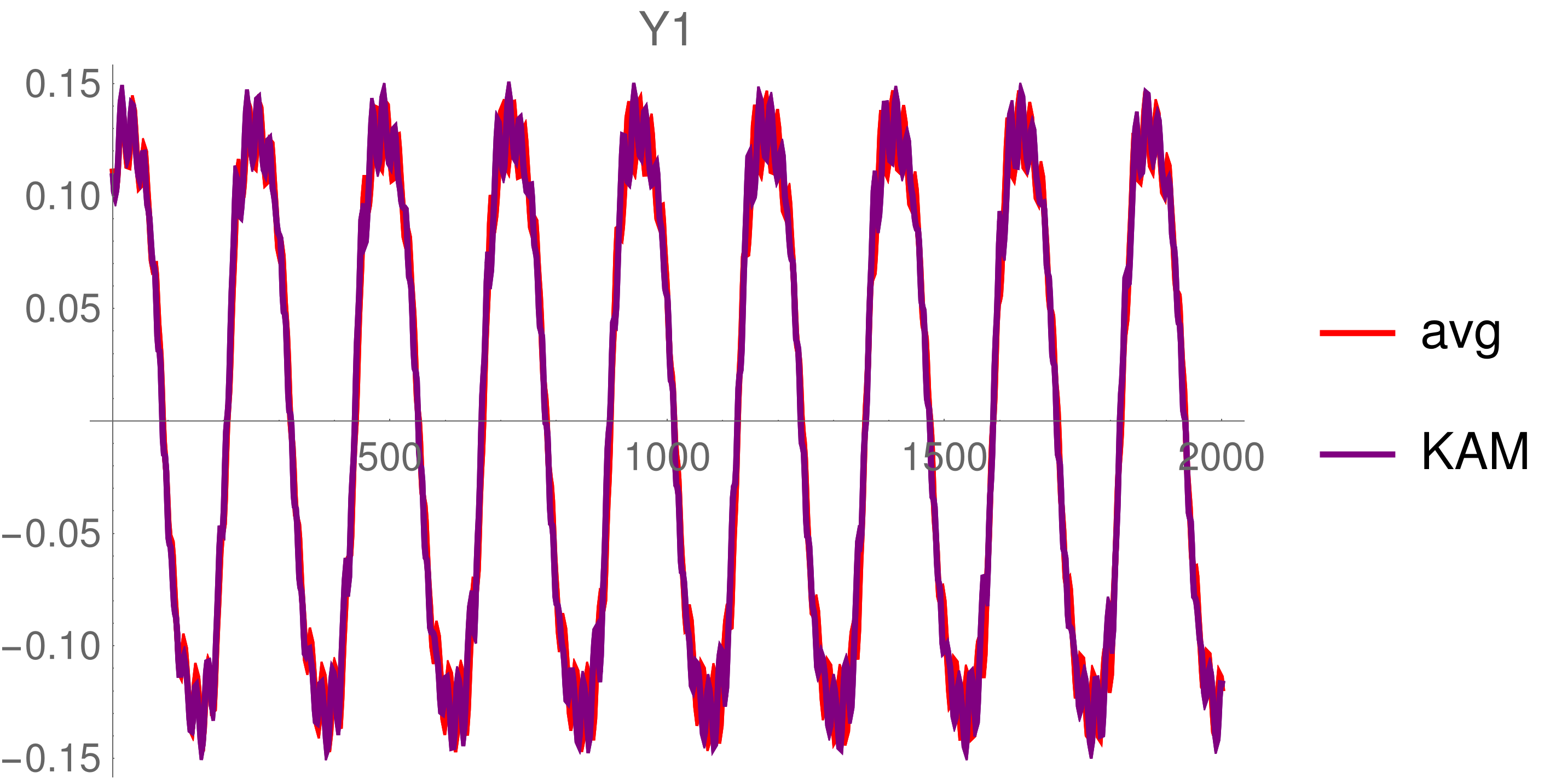
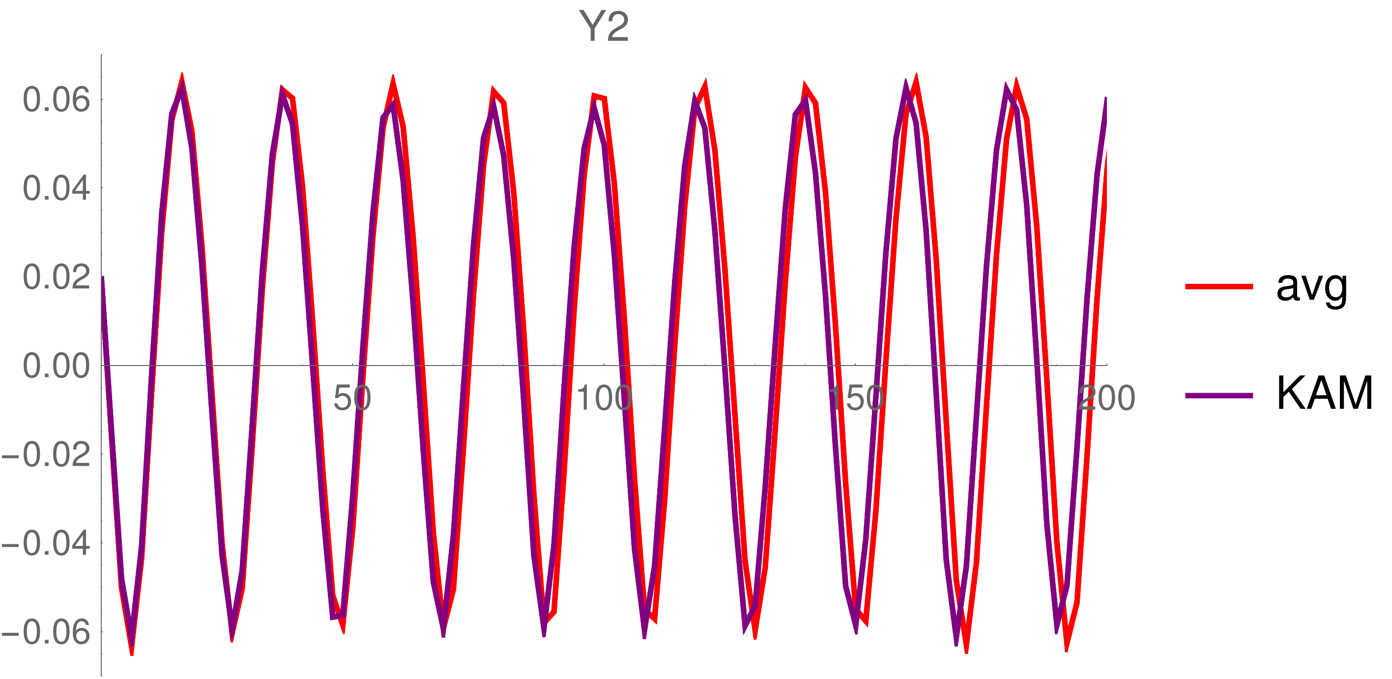
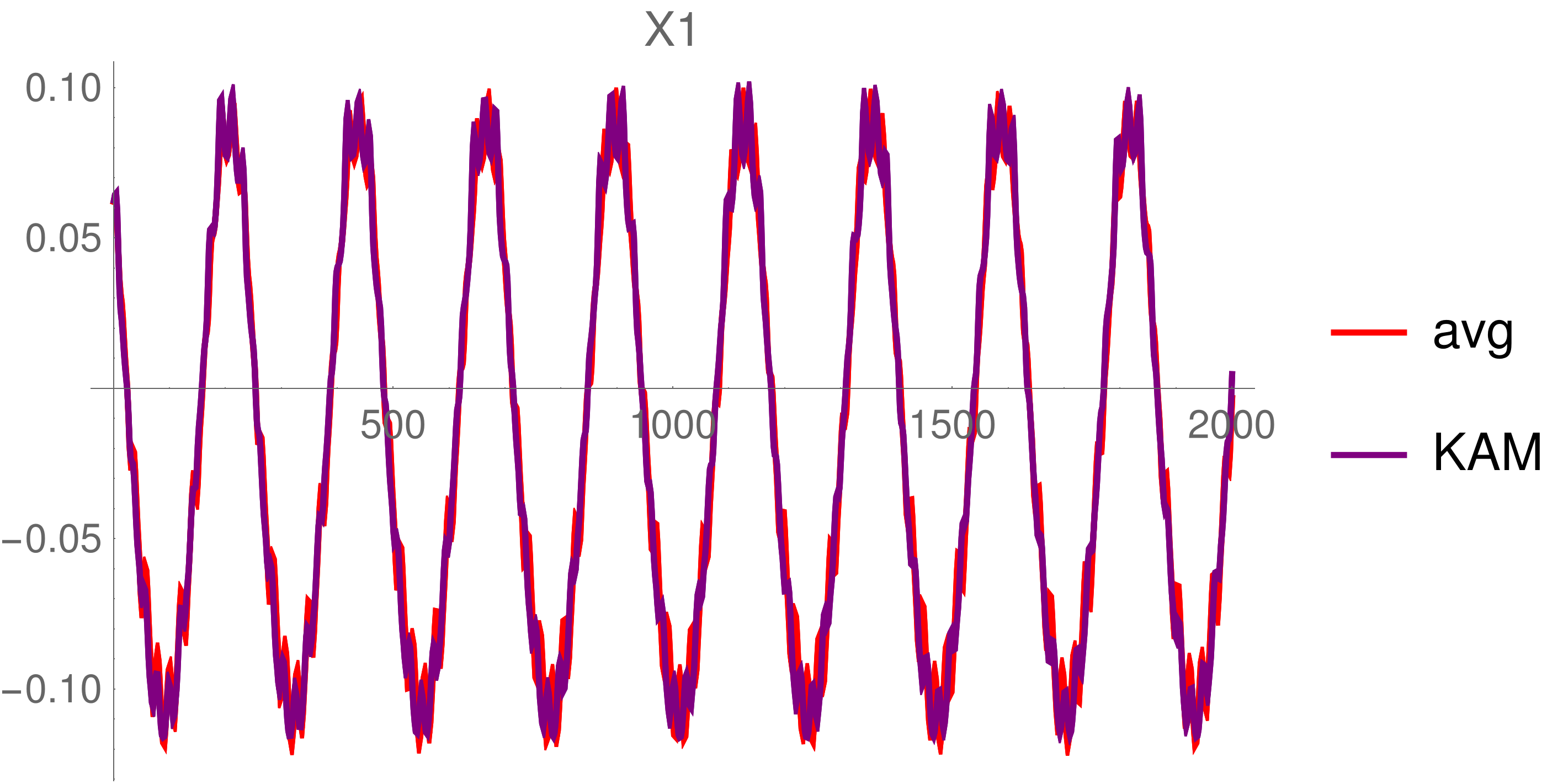
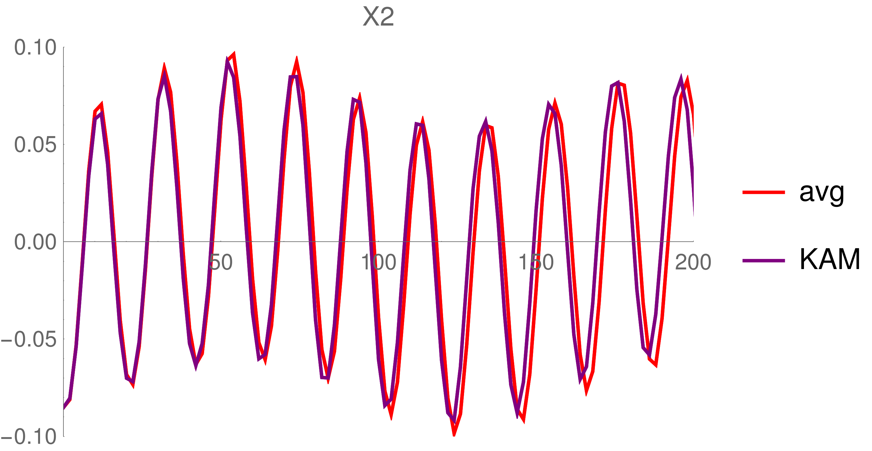
Figure 8: Evolutions with respect to time [yr] of the secular variables (reported in the panels on the left) and the relatively faster ones (in the right panels) in our model of the MMR librational dynamics of HD60532. They are given by the semi-analytic solutions of the averaged Hamiltonian up to order $6$ (red curves) and the Hamiltonian that is produced after $5$ steps of the Kolmogorov normalization algorithm (purple curves).

The plots in Fig. 8 show an excellent superimposition between the two solutions, with respect to both the amplitudes and the frequencies. This makes evident the effectiveness of our computational algorithm. Let us also recall that the initial conditions $(\bm{Y}(0),\bm{X}(0))$ are the ones compatible with the observations.

6.2 Computer-assisted proof

By looking at the plots in Fig. 7, it can be noticed that the decrease of the norms of the generating functions, in particular for what concerns the finite sequence of the second generating function $\chi_{1}^{(r)}$, is not so regular and the convergence of the algorithm looks doubtful. In order to rigorously prove that the KAM algorithm is convergent, we adopt a rigorous approach based on a computer-assisted proof. For this purpose, we follow the method which has been described in [6] and further developed in [35], where a publicly available software package is provided as supplementary material. Such a package is designed for doing just this kind of computer-assisted proof for Hamiltonian systems having two degrees of freedom. In order to use this software so as to apply it to the problem under consideration, it is just matter to prepare some input files, which basically describe the starting Hamiltonian; in principle, this can allow us to prove the existence of the KAM torus we are aiming at, if the corresponding Kolmogorov normal form is close enough to such an initial Hamiltonian. More precisely, we consider $H^{(5)}$ as the starting Hamiltonian. It is fully determined at the end of the application of the Newton method, which has been described in the previous Section; in terms of a single mathematical formula, it can be written as

$$H\circ\mathcal{A}\circ\mathcal{C}^{(5)}\circ\mathcal{T}_{\tilde{I}_{1}}\circ\mathcal{K}^{(5)}$$

where $H$, $\mathcal{A}$, $\mathcal{C}^{(5)}$, $\mathcal{T}_{\tilde{I}_{1}}$ and $\mathcal{K}^{(5)}$ are defined in (1), (2), (6), just below formula (20) and (19), respectively. Moreover, the expansion of $H^{(5)}$ can be written as in (18) and is truncated up to degree $2$ in the actions and to trigonometrical degree $12$ in the angles, while the expansion (5) of the intermediate Hamiltonian $\mathcal{H}^{(5)}=H\circ\mathcal{A}\circ\mathcal{C}^{(5)}$ has been preliminarly truncated so as to exclude the sum of terms $\sum_{\ell>6}h_{\ell}^{(r)}(\bm{J},\bm{\vartheta})=\mathcal{O}\big{(}\|\bm{J}\|^{7/2}\big{)}$. Therefore, $H^{(5)}$ is not in Kolmogorov normal form because of a few (small) Hamiltonian terms that are either dependent on the angles $\bm{q}$ only or linearly dependent on the actions $\bm{p}$.

During the initial stage of the computer-assisted proof, a first code explicitly performs a (possibly large) number $R_{\rm I}$ of normalization steps of a classical formulation of the Kolmogorov algorithm, which includes also small translations of the actions that aim at keeping fixed the desired angular velocity vector of the quasi-periodic motion on the final torus, i.e., $\bm{\omega}^{*}$. Afterwards, the size of the perturbation is further reduced (although in a less efficient way) by another code which just iterates the estimates of the norms of the terms of order $r$ with $R_{\rm I}<r\leq R_{\rm II}$. In the case of the model we are studying, in order to achieve the convergence of the algorithm, we have found convenient to set $R_{\rm I}=200$ and $R_{\rm II}=20\,000$. The whole computer-assisted proof required a total computational time of about $52.5$ hours on a workstation equipped with CPUs of type Intel XEON-GOLD 5220 (2.2 GHz) and 384 GB of RAM. Nearly all the time (i.e., more than 50 hours) has been requested by the first explicit computation of the (truncated) expansions of the Hamiltonians $H^{(r)}$ for $r=1\,,\,\ldots\,,\,R_{I}=200$.

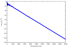
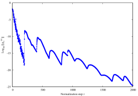
Figure 9: Estimates of the norms of the generating functions $\chi_{1}^{(r)}$, as they are evaluated during the computer-assisted proof, up to order $R_{\rm II}=20\,000$ (left panel). In the right panel, the zoom of the estimates of $\big{\|}\chi_{1}^{(r)}\|$ produced by the first $2\,000$ normalization steps.

The plot of the norms of the generating functions $\chi_{1}^{(r)}$ (in semi-log scale) is reported in Fig. 9, where the occurrence of a regular decrease is clearly highlighted. In particular, looking at the panel on the right, we can appreciate that the decrease is sharper for the first $R_{\rm I}$ normalization steps, where the expansions of the generating functions are computed explicitly. Afterwards, there is a transition to the regime of the iteration of the norms and, after some initially periodic jumps, the decrease becomes more regular.

At the end of the running of the codes which make part of the software package designed to perform this kind of computer-assisted proofs, upper bounds for all the terms appearing in the expansion of $H^{(R_{\rm II})}$, which is written as in (18), are available. Therefore, one can check in an automatic way the applicability of the KAM theorem (e.g., in the version proved in [34], which fits perfectly in this framework). The application of all this computational procedure allows us to prove our final result, that is summarized in the following statement.

Theorem 6.1 (Computer-assisted)

Let us consider the Hamiltonian $H^{(5)}$, expanded as in (18) and truncated up to degree $2$ in the actions and to trigonometrical degree $12$ in the angles. Let $\bm{\omega}^{*}\in{\mathbb{R}}^{2}$ be such that

$$\omega_{1}^{*}\in\left(-2.72805620345077182\times 10^{-2},-2.72805620345057182\times 10^{-2}\right)$$

$$\omega_{2}^{*}\in\left(-3.0574227066998818\times 10^{-1},-3.0574227066978818\times 10^{-1}\right)$$

and it satisfies the Diophantine condition

$$|\bm{k}\cdot\bm{\omega}^{*}|\geq\frac{\gamma}{|\bm{k}|^{\tau}}\ ,\quad\forall\,\bm{k}\in{\mathbb{R}}^{2}\setminus\{0\}\ ,$$

with $\gamma=2.7280562034505684\times 10^{-2}$ and $\tau=1$. Therefore, there exists an analytic canonical transformation which transforms the Hamiltonian $H^{(5)}$ in the Kolmogorov normal form (12). In the new action-angle coordinates, the torus $\{\bm{p}=\bm{0}\,,\ \bm{q}\in\mathbb{T}^{2}\}$ is invariant and carries quasi-periodic orbits whose corresponding angular velocity vector is $\bm{\omega}^{*}$.

References

- [1] A.J. Alves, T.A. Michtchenko, M. Tadeu dos Santos. Dynamics of the 3/1 planetary mean-motion resonance: an application to the HD60532 b-c planetary system. Cel. Mech. & Dyn. Astr., 124, 311–334 (2016).
- [2] K. Batygin, A. Morbidelli. Analytical treatment of planetary resonances A&A, 556, A28 (2013).
- [3] R.P. Butler, G.W. Marcy, D.A. Fischer, T.M. Brown, A.R. Contos, S.G. Korzennik, P. Nisenson, R.W. Noyes. Evidence for Multiple Companions to Andromedæ. Astroph. Jour., 526, 916–927 (1999).
- [4] C. Caracciolo, U. Locatelli. Computer-assisted estimates for Birkhoff normal forms. Journal of Computational Dynamics, 7, 425–460 (2020).
- [5] C. Caracciolo, U. Locatelli, M. Sansottera, M. Volpi. Librational KAM tori in the secular dynamics of the Andromedæ planetary system. MNRAS, 510, 2147–2166 (2022).
- [6] A. Celletti, A. Giorgilli, U. Locatelli. Improved estimates on the existence of invariant tori for Hamiltonian systems. Nonlinearity, 13, 397–412 (2000).
- [7] R. Deitrick, R. Barnes, B.E. McArthur, T.R. Quinn, R. Luger, A. Antonsen, G.F. Benedict. The Three–Dimensional Architecture of the Andromedæ. Astroph. Jour., 798:46 (2015).
- [8] J.-Ll. Figueras, A. Haro and A. Luque. Rigorous computer-assisted application of KAM theory: a modern approach. Found. Comput. Math., 17 (2017), 1123–1193.
- [9] F. Gabern, A. Jorba, U. Locatelli. On the construction of the Kolmogorov normal form for the Trojan asteroids. Nonlinearity, 18, 1705–1734 (2005).
- [10] A. Giorgilli. Notes on Hamiltonian Dynamical Systems. London Mathematical Society Student Texts, 102, ISBN: 9781009151139 (2022).
- [11] A. Giorgilli, A. Delshams, E. Fontich, L. Galgani, C. Simó. Effective stability for a Hamiltonian system near an elliptic equilibrium point, with an application to the restricted three–body problem. J. Differential Equations, 77, 167–198 (1989).
- [12] A. Giorgilli, U. Locatelli, M. Sansottera. Kolmogorov and Nekhoroshev theory for the problem of three bodies. Cel. Mech. & Dyn. Astr., 104, 159–173 (2009).
- [13] A. Giorgilli, U. Locatelli, M. Sansottera. Secular dynamics of a planar model of the Sun-Jupiter-Saturn-Uranus system; effective stability in the light of Kolmogorov and Nekhoroshev theories. Reg. & Chaotic Dyn., 22, 54–77 (2017).
- [14] A. Giorgilli, M. Sansottera. Methods of algebraic manipulation in perturbation theory. In P.M. Cincotta, C.M. Giordano, C. Efthymiopoulos (eds.): “Chaos, Diffusion and Non-integrability in Hamiltonian Systems – Applications to Astronomy”, Proceedings of the Third La Plata International School on Astronomy and Geophysics, Universidad Nacional de La Plata and Asociación Argentina de Astronomía Publishers, La Plata (2012).
- [15] W. Gröbner. Die Lie-Reihen und Ihre Anwendungen. Springer Verlag, Berlin (1960). Italian transl. in Le serie di Lie e le loro applicazioni. Cremonese, Roma (1973).
- [16] S. Hadden. An Integrable Model for the Dynamics of Planetary Mean-motion Resonances. Astron. Jour., 158:238 (2019).
- [17] A. Haro, M. Canadell, J-LL. Figueras, A. Luque, J-M. Mondelo. The parameterization method for invariant manifolds. Applied Mathematical Sciences, vol. 195, Springer (2016).
-
[18]
J. Laskar.
Les variables de Poincaré et le
développement de la fonction perturbatrice. Groupe de travail
sur la lecture des Méthodes nouvelles de la Mécanique
Céleste.
Notes scientifiques et techniques du Bureau des
Longitudes, S026
(1989).
https://www.imcce.fr/content/medias/publications/publications
-recherche/nst/docs/S026.pdf - [19] J. Laskar. Frequency map analysis and quasi periodic decompositions. In D. Benest, C. Froeschlé, & E. Lega E. (eds.), Hamiltonian systems and Fourier analysis, Taylor and Francis, Cambridge (2003)
- [20] J. Laskar, A. C. M. Correia. HD 60532, a planetary system in a 3:1 mean motion resonance. Astron. & Astroph., 496, L5–L8 (2009).
- [21] J. Laskar, P. Robutel. High order symplectic integrators for perturbed Hamiltonian systems. Cel. Mech. & Dyn. Astr., 80, 39–62 (2001).
- [22] A.-S. Libert, M. Sansottera. On the extension of the Laplace-Lagrange secular theory to order two in the masses for extrasolar systems. Cel. Mech. & Dyn. Astr., 117, 149–168 (2013).
- [23] U. Locatelli, C. Caracciolo, M. Sansottera, M. Volpi. A numerical criterion evaluating the robustness of planetary architectures; applications to the Andromedæ system In A. Celletti, C. Galeş, C. Beaugé, A. Lemaitre, eds., Multi-scale (time and mass) dynamics of space objects, Proceedings of the International Astronomical Union Symposium No. 364, Book Series, Volume 15, Pages 65-84, DOI 10.1017/S1743921322000461 (2021).
- [24] U. Locatelli, C. Caracciolo, M. Sansottera, M. Volpi. Invariant KAM tori: from theory to applications to exoplanetary systems In G. Baù, S. Di Ruzza, R.I. Páez, T. Penati & M. Sansottera (eds.), I-CELMECH Training School — New frontiers of Celestial Mechanics: theory and applications, Springer PROMS, volume 399, eBook ISBN 978-3-031-13115-8 (2022).
- [25] U. Locatelli, A. Giorgilli. Invariant tori in the secular motions of the three–body planetary systems. Cel. Mech. & Dyn. Astr., 78, 47–74 (2000).
- [26] U. Locatelli, A. Giorgilli. Construction of the Kolmogorov’s normal form for a planetary system. Reg. & Chaot. Dyn., 10, 153–171 (2005).
- [27] U. Locatelli, A. Giorgilli. Invariant tori in the Sun–Jupiter–Saturn system. Discr. & Cont. Dyn. Sys. — B, 7, 377–398 (2007).
- [28] B.E. McArthur, G.F. Benedict, R. Barnes, E. Martioli, S. Korzennik, E. Nelan, R.P. Butler. New observational constraints on the Andromedæ system with data from the Hubble Space telescope and Hobby-Eberly telescope. Astroph. Jour., 715, 1203–1220 (2010).
- [29] T.A. Michtchenko, R. Malhotra. Secular Dynamics of the Three-Body Problem: Application to the Andromedæ Planetary System. Icarus, 168, 237–248 (2004).
- [30] F. Mogavero, J. Laskar. The origin of chaos in the Solar System through computer algebra Astron. & Astroph., 662, L3 (2022).
- [31] A. Morbidelli, A. Giorgilli. Superexponential stability of KAM tori. J. Stat. Phys., 78, 1607–1617 (1995).
- [32] G. Pucacco. Normal forms for the Laplace resonance. Cel. Mech. & Dyn. Astr., 133:3 (2021).
- [33] M. Sansottera, A.-S. Libert. Resonant Laplace-Lagrange theory for extrasolar systems in mean-motion resonance. Cel. Mech. & Dyn. Astr., 131:38 (2019).
- [34] L. Stefanelli , U. Locatelli. Kolmogorov’s normal form for equations of motion with dissipative effects. Discr. & Cont. Dyn. Sys. — B, 17, 2561–2593 (2012).
- [35] L. Valvo, U. Locatelli. Hamiltonian control of magnetic field lines: Computer assisted results proving the existence of KAM barriers. Journal of Computational Dynamics, 9, 505–527 (2022).
- [36] M. Volpi, U. Locatelli, M. Sansottera. A reverse KAM method to estimate unknown mutual inclinations in exoplanetary systems. Cel. Mech. & Dyn. Astr., 130:36 (2018).
- [37] M. Volpi, A. Roisin, A.-S. Libert. On the 3D secular dynamics of radial-velocity-detected planetary systems. Astron. & Astroph., 626, A74 (2019).