Composite Sorting

Abstract

We propose a new sorting framework: composite sorting. Composite sorting comprises of (1) distinct worker types assigned to the same occupation, and (2) a given worker type simultaneously being part of both positive and negative sorting. Composite sorting arises when fixed investments mitigate variable costs of mismatch. We completely characterize optimal sorting and additionally show it is more positive when mismatch costs are less concave. We then characterize equilibrium wages. Wages have a regional hierarchical structure $-$ relative wages depend solely on sorting within skill groups. Quantitatively, composite sorting can generate a sizable portion of within-occupations wage dispersion in the US.

JEL-Codes: J01, D31, C78
Keywords: Composite Sorting, Assignment

1 Introduction

Sorting models have a prominent position in economics (Koopmans:1957; Becker:1973). An important insight of this literature is that when the output function is supermodular or submodular, sorting is positive or negative, implying that very similar or identical worker types work in the same occupation. Sattinger:1993, Chiappori:2016, Chade:2017, and Eeckhout:2018 provide comprehensive reviews of this literature.

Our paper provides the first complete characterization of optimal sorting and wages in a sorting model with an output function that is neither supermodular nor submodular. We establish that equilibrium sorting is significantly richer than in the canonical settings, yet we characterize it fully. We call the sorting pattern that emerges composite sorting. Composite sorting has two main features. First, distinct workers are sorted to the same occupation. This enables us to study wage dispersion within occupations. Second, a given worker type can simultaneously be in both positive and negative sorting. We theoretically characterize optimal sorting, its comparative statics, and a dual solution. We then present an example that captures defining features of the theoretical characterization and quantitatively demonstrate our model using American Community Survey data. The example generates 29 percent of overall wage dispersion and about 50 percent of wage dispersion at the top and the bottom of the wage distribution. In contrast, with either supermodular or submodular costs, the solution is positive or negative one-to-one sorting with no dispersion in wages.

We study a sorting model with heterogeneous workers, heterogeneous jobs, and mismatch. Mismatch is the difference between the skill of the worker and the difficulty of the job. When the job’s difficulty exceeds the worker’s skill level, that is, when a worker is underqualified, mismatch decreases output. The second type of mismatch (as in Lise:2020) arises when the worker’s ability surpasses the job’s demands, that is, when the worker is overqualified, resulting in a utility loss for a worker and a corresponding loss in the joint surplus. Following Stigler:1939 and Laffont:1986; Laffont:1991, firms can incur fixed costs to reduce the variable costs of mismatch. Firms mitigate adverse effects of mismatch by investing in technologies or providing amenities. An example of such mitigation is investing in a cobot (collaborative robot) that enhances the output of a low-skill welder. The result of the technology decision is that the cost of mismatch is concave in the extent of underqualification. Similarly, employers may invest in amenities to decrease the disutility of workers (as in Rosen:1986) when they are overqualified. An example of such mitigation is investing in a premium truck with advanced comfort and drivers support system for a high-skill trucker. The result of investment in amenities is that the cost of mismatch is concave in the extent of overqualification. In sum, the cost of mismatch is concave in mismatch. The key characteristic of a generic concave function in mismatch is that it is neither supermodular nor submodular. We are able to provide a complete characterization of this sorting problem with neither supermodular nor submodular output by analyzing it using the tools of optimal transport theory.

We now describe the main features of an optimal assignment. First, an optimal assignment maximizes the number of perfect pairs, which are pairs without mismatch. Since mismatch costs are concave, it is preferable to have a combination of one pair with small mismatch and another with significant mismatch, as opposed to having two pairs with moderate mismatch. A combination of a perfect pair and a pair with significant mismatch exemplifies this.

Figure 1: Pairings Between Workers and Jobs Do Not Intersect

Figure 1 illustrates that for an optimal sorting, pairings between workers and jobs do not intersect. Positive sorting, in the left panel, pairs a low-skill worker and a high-skill job $(x_{L},z_{H})$, and a medium-skill worker with an exceptional skill job $(x_{M},z_{E})$, resulting in two medium-size mismatches. For concave costs, instead, it is preferable to have one large mismatch $(x_{L},z_{E})$ and one small mismatch $(x_{M},z_{H})$. It is optimal to have pairs that do not intersect as in the right panel.

The second feature of an optimal assignment is that pairings between workers and jobs do not intersect. Consider workers with low and medium skills $\{x_{L},x_{M}\}$ and jobs that require high and exceptional skills $\{z_{H},z_{E}$}. Positive sorting assigns the low-skill worker to the high-skill job $(x_{L},z_{H})$, and the medium-skill worker to the exceptional job $(x_{M},z_{E})$. This results in two medium-size mismatch costs. Visualizing the pairing as arcs connecting a worker with a job reveals that the pairs intersect as in the left panel of Figure 1. For concave costs, in contrast, it is preferable to have one large mismatch (between a low-skill worker and a very high-skill job $(x_{L},z_{E})$) and one small mismatch (between a medium-skill worker and a high-skill job $(x_{M},z_{H})$). Thus, it is optimal to have pairs that do not intersect as in the right panel.

The feature of no intersecting pairs gives rise to two additional properties of optimal sorting. First, the assignment problem can be decomposed into independent problems by layers. Layers are constructed by first designing a measure of underqualification that evaluates the cumulative deficiency of worker skills compared to the cumulative demands of jobs at a given skill level. A layer contains all the workers and jobs in a particular slice of this measure of underqualification. An assignment in each layer optimally pairs workers and jobs within a given slice (given the same mismatch cost function), independent of all workers and jobs in other layers. The full optimal assignment sums the optimal assignments of each layer. Second, we characterize an optimal assignment within a given layer through a Bellman equation.

Figure 2: An Example of Composite Sorting

Figure 2 explains composite sorting with four workers (circles) and four jobs (dots). In the top panel, workers are optimally assigned to jobs in their skill group which results in two positively sorted pairs: $(x_{L},z_{L})$ and $(x_{H},z_{H})$. Adding an identical low-skill worker and an identical high-skill job does not allow to reduce the initial mismatch and results in a pair $(x_{L},z_{H})$. The medium worker-job group $\{x_{M},z_{M}\}$ can be used to rematch the low-skill worker and the high-skill job with the medium-skill job and worker forming pairs $(x_{L},z_{M})$ and $(x_{M},z_{H})$, but such reshuffling is not optimal due to the concavity of the costs. In the bottom panel, we hence also have two negatively sorted pairs $(x_{L},z_{H})$ and $(x_{M},z_{M})$ which delivers composite sorting (observe that worker type $x_{L}$ is assigned to distant occupations; not to $z_{M}$).

The main result of our paper is composite sorting $-$ the optimal assignment sorts identical workers into different jobs, some positively and some negatively. The intuition for composite sorting can be described through an example. Suppose a low worker-job group $\{x_{L},z_{L}$} is far from a high worker-job group $\{x_{H},z_{H}$} as in the top panel of Figure 2. When there is a significant gap between the groups, workers are optimally assigned to jobs within their skill groups resulting in two pairs $(x_{L},z_{L})$ and $(x_{H},z_{H})$. This results in two small mismatches and positive sorting. Suppose one identical low-skill worker $x_{L}$ and one identical high-skill job $z_{H}$ as well a medium-skill worker-job group $\{x_{M},z_{M}$} are added as in the bottom panel of Figure 2. Adding an identical low-skill worker and an identical high-skill job does not allow to reduce the initial mismatched pairs $(x_{L},z_{L})$ and $(x_{H},z_{H})$, and so the added low-skill worker is assigned to the added high-skill job forming a pair $(x_{L},z_{H})$. The medium worker-job group $\{x_{M},z_{M}$} can, in principle, be used to rematch the added low-skill worker and the added high-skill job with the medium-skill job and worker forming pairs $(x_{L},z_{M})$ and $(x_{M},z_{H})$. However, such reshuffling is not optimal, because due to concavity of the costs, two medium mismatches $(x_{L},z_{M})$ and $(x_{M},z_{H})$ are worse than one small mismatch within the medium-skill group $(x_{M},z_{M})$ and one large mismatch for $(x_{L},z_{H})$. As a result, the medium-skill group is paired together and this results in the negative sorting within the added group.

We emphasize that composite sorting assigns the same worker type to very different occupations, with some positive and some negative sorting. In the example, the low-skill worker $x_{L}$ is paired positively with the low-skill occupation $z_{L}$ (as a part of the sorting $(x_{L},z_{L})$ and $(x_{H},z_{H})$) but the same worker type is also paired negatively to the distant high-skill occupation $z_{H}$ (as a part of the sorting $(x_{L},z_{H})$ and $(x_{M},z_{M})$). Thus, the optimal full assignment is not one-to-one between types because the same worker type is assigned to different occupations as a part of simultaneously positive and negative sorting.

For general distributions, composite sorting may be very rich with very distinct worker types being assigned to the same occupation and may exhibit various local and global intervals of positive and negative sorting. We show how to completely characterize optimal sorting for general distributions.

We next analyze how these rich sorting patterns vary with changes in technology. In comparative statics analysis, we derive that sorting becomes more positive, by which we mean larger in concordance order, as the cost of mismatch becomes less concave. With a fixed pair of worker and job distributions, the assignment problem is split into a fixed set of layers irrespective of the cost function, and we show that for each layer sorting becomes more positive as the cost of mismatch becomes less concave. Moreover, we show that there exists a threshold of concavity for the cost function above which the optimal sorting within each layer is positive.

We determine equilibrium wages and firm values by characterizing the solution to the dual planning problem. We show that wages and job values exhibit a regional hierarchical structure. For a given skill group, relative wages are determined regionally; that is, they depend only on information within the regional skill group and do not depend on any other groups. The hierarchical structure aggregates the regional relative wages to wages for larger groups preserving the relative wages implied by the smaller regions.

An important implication of our results is frictionless wage dispersion within occupations. We develop an example that captures essential features of the complete characterization of composite sorting, and we investigate to what extent it can generate qualitative and quantitative patterns of wage dispersion in the American Community Survey. We find that the model delivers sizable wage dispersion within occupations with high and low mean wages. Composite sorting can generate 54 percent of wage dispersion within jobs at the bottom of the distribution, and 59 percent at the top. The model can generate 10 percent of wage dispersion in the middle of the distribution. The main reason is that the logarithmic wage profile is relatively flat in this range and, even though there may be substantial skill dispersion within a particular occupation, it does not give rise to substantial wage dispersion. Overall, composite sorting accounts for 29 percent of the wage dispersion in the sample. In contrast, one-to-one sorting models (such as models with positive or negative sorting arising from submodular or supermodular costs) would deliver no wage dispersion within occupations.

Literature. We briefly discuss additional relevant literature. Kremer:1996 and Porzio:2017 study sorting of heterogeneous workers with a form of technology choice where there is selection in managerial and worker roles. Anderson:2022 depart from focusing on the conditions for assortative sorting by developing comparative statics for assortative sorting without having to solve for the optimal assignment. Chiappori:2022 and Fagereng:2022 analyze non-assortative sorting patterns in income and wealth. Another recent development in the assignment literature is to study models with multiple agents combined together (Kremer:1993; Chiappori:2017; Chade:2018; Eeckhout:2018b; BTZ:2021).

A general alternative that results in imperfect assortative sorting is the search and matching literature (for example, Shimer:2000, Postel:2002, Cahuc:2006, Eeckhout:2010, Lise:2017, Bagger:2019). Specifically, this approach generates wage dispersion within occupations due to the search frictions. Our work instead generates wage dispersion in a frictionless environment.

Our paper uses results from the optimal transport literature (see Galichon:2018 for a comprehensive overview of applications of optimal transport theory to economic problems). In the optimal transport literature the idea of perfect pairs is referred to as “mass stays in place if it can” (Gangbo:1996; Villani:2003). Villani:2009 states that the non-intersecting rule first appears in Monge:1781. This non-intersecting property is central to the literature on optimal transport with concave distance costs as well as to algorithmic sorting problems with distance costs (Werman:1986; Aggarwal:1995). Aggarwal:1995 proposed the first combinatorial algorithm that can be used to solve for an optimal assignment within a layer when the cost of mismatch is linear. The Bellman equation in our papers adopts a recursive algorithm developed by Nechaev:2013, designed to model statistical properties of polymer chains. The idea of layering was introduced in Delon:2012b. Their work also develops a more computationally efficient version of the Bellman equation building on Aggarwal:1995. We provide a new, concise proof of this more efficient Bellman equation that also extends to case of asymmetric mismatch cost functions. Our comparative statics results for the primal problem and a complete characterization of the dual solution and its regional hierarchical structure are also a contribution to the optimal transport theory and, more specifically, to the literature with concave distance costs started by Gangbo:1996 and McCann:1999.

2 Model

We study an environment in which workers with heterogeneous skills sort into heterogeneous jobs, and where mismatch between their skills and the job difficulty leads to output losses. Firms mitigate the extent to which mismatch penalizes surplus by reducing variable mismatch costs with fixed cost investments.

2.1 Environment

The economy is populated by risk-neutral workers and jobs. The workers differ in their skills which are indexed by $x$. The set of worker skills $X$ contains a finite number $n$ of types $x_{1}<x_{2}<\dots<x_{n}$. Workers are distributed according to the cumulative distribution function $F(x)$.

Jobs differ in their difficulty which is indexed by $z$. The set of occupations $Z$ contains a finite number $m$ of occupation types $z_{1}<z_{2}<\dots<z_{m}$. Jobs are distributed according to the cumulative distribution function $G(z)$.

Surplus. Firms produce a single good. Production requires one worker for each job. Since both workers and firms are risk-neutral, what matters is the surplus generated by a worker-job pair $(x,z)$. The surplus generated by a worker with skill $x$ in an occupation with difficulty level $z$ is:

$$s(x,z)=g(x)+h(z)-\gamma_{p}\max(z-x,0)-\gamma_{u}\max(x-z,0),$$ (1)

with $\gamma_{p},\gamma_{u}\geqslant 0$. There are four terms in this technology specification. The first term $g(x)$ with $g^{\prime}(x)>0$ reflects that a more skilled worker contributes more to production, independent of the job. The second term $h(z)$ where $h^{\prime}(z)>0$ reflects that a more difficult job $z$ produces more output and is thus more valuable, independent of the worker that fulfills the job. The third term $\gamma_{p}\max(z-x,0)$ captures the idea that a worker with a skill $x$ that is lower than the job demand $z$ causes a loss of output. It is costly to have workers perform tasks for which they have limited talent. The fourth term $\gamma_{u}\max(x-z,0)$ captures the idea that a worker with skills $x$ that exceed the job demands $z$ is overqualified and needs to be compensated for their utility cost (as in Rosen:1986 and Lise:2020). Mismatch is the distance between worker skill $x$ and job difficulty $z$.

Technology Choice. We assumed so far that mismatch costs of a worker-job pair $(x,z)$ are exogenous. We next endogenize the mismatch costs. A firm can reduce the costs of mismatch by making a fixed investment. In case a worker is underqualified, the firm can make technology investments to reduce the production costs of mismatch. When workers are overqualified, the firm can provide amenities to reduce the utility costs of mismatch. The main insight of Stigler:1939 and Laffont:1986; Laffont:1991 is that this technology choice results in an effective output function with a concave cost of mismatch.

We model technology choice as a firm making fixed investments (for example, by purchasing better equipment) to reduce variable costs associated with mistakes and delays caused by a worker that is underqualified to fulfill the job, $x<z$. Specifically, firms choose the variable cost of production mismatch $\gamma_{p}$, which comes at an associated fixed cost $\Psi_{p}(\gamma_{p})=\frac{1}{\eta_{p}}\gamma_{p}^{-\eta_{p}}$, where $\eta_{p}$ is strictly positive. By decreasing variable costs $\gamma_{p}$, the firm increases its fixed costs, or $\Psi_{p}^{\prime}<0$, where $\Psi_{p}^{\prime\prime}>0$. The effective output of worker $x$ in occupation $z>x$ is then:

$$y(x,z)=\max_{\gamma_{p}\geqslant 0}\;\bigg{(}g(x)+h(z)-\gamma_{p}(z-x)-\frac{1}{\eta_{p}}\gamma_{p}^{-\eta_{p}}\bigg{)}.$$ (2)

Investment increases in the distance between the worker skill and the job difficulty $-$ the technology choice is $\gamma_{p}=(z-x)^{-\frac{1}{1+\eta_{p}}}$. Firms choose a low variable cost of production mismatch if the worker is less qualified, that is, when the distance between skills and demands $(z-x)$ is large.

The effective output of worker $x$ in job $z$ is, using the technology investment decision, given by:

$$y(x,z)=g(x)+h(z)-\frac{1}{\zeta_{p}}(z-x)^{\zeta_{p}}$$ (3)

for underqualified workers $x<z$, with $\zeta_{p}=\frac{\eta_{p}}{1+\eta_{p}}\in(0,1)$. The distinctive feature of this function is that the mismatch cost is concave in the distance between worker skill and job difficulty. In sum, the technology choice transforms a production function with linear mismatch costs into an effective output function with strictly concave mismatch costs.

Firms can similarly reduce the extent to which overqualificaton penalizes worker utility by providing amenities. We model amenity choices analogous to technology choices. When workers are overqualified, $x>z$, their employers want to invest in amenities to lower the disutility from working. Firms choose the variable utility cost due to mismatch $\gamma_{u}$ at an associate fixed cost $\Psi_{u}(\gamma_{u})=\frac{1}{\eta_{u}}\gamma_{u}^{-\eta_{u}}$, where $\eta_{u}$ is strictly positive. The provision of amenities is thus characterized by $\gamma_{u}=(x-z)^{-\frac{1}{1+\eta_{u}}}$. Amenities increase with worker skills. As a result, the effective output of overqualified workers is $y(x,z)=g(x)+h(z)-\frac{1}{\zeta_{u}}(x-z)^{\zeta_{u}}$, with $\zeta_{u}=\frac{\eta_{u}}{1+\eta_{u}}\in(0,1)$.

Effective Output. We write effective output as:

$$y(x,z)=g(x)+h(z)-\begin{cases}\frac{1}{\zeta_{p}}(z-x)^{\zeta_{p}}\hskip 130.88284pt\text{ if }z\geqslant x\\ \frac{1}{\zeta_{u}}(x-z)^{\zeta_{u}}\hskip 130.59804pt\text{ if }z<x,\end{cases}$$ (4)

where $\zeta_{p},\zeta_{u}\in(0,1)$. We use effective output (4) to define the cost of mismatch between worker $x$ and job $z$ as:

$$c(x,z)=g(x)+h(z)-y(x,z)=\begin{cases}\frac{1}{\zeta_{p}}(z-x)^{\zeta_{p}}\hskip 85.35826pt\text{ if }z\geqslant x\\ \frac{1}{\zeta_{u}}(x-z)^{\zeta_{u}}\hskip 85.07388pt\text{ if }z<x,\end{cases}$$ (5)

that is, maximal output of worker $x$ and job $z$ minus effective output $y(x,z)$. Thus, the mismatch cost function is concave in the discrepancy between worker $x$ and job $z$. We plot an example of the mismatch cost function in Figure 3.

Figure 3: The Cost of Mismatch

Figure 3 illustrates the cost of mismatch $c(x,z)$, which is concave in the discrepancy between the worker skill $x$ and the job difficulty $z$. The result of the firm technology decision is that the mismatch cost function is concave in the extent of underqualification $(z-x)$. The result of investment in amenities is that the mismatch cost function is concave in the extent of overqualification $(x-z)$.

The output function is neither supermodular nor submodular. First, the cross-derivatives of the output function being negative for both $z>x$ and $z<x$ directly rules out supermodularity. Second, the output function is not submodular. Consider two workers and two jobs, each with skills $a$ and $b$ where $b\neq a$. Submodularity requires the combined output of pairs $(a,b)$ and $(b,a)$ to be greater than the combined output of pairs $(a,a)$ and $(b,b)$. However, pairs $(a,b)$ and $(b,a)$ have mismatch and consequently lower output than the positive sorting $(a,a)$ and $(b,b)$ which gives zero mismatch. Thus, the output function is not submodular either.

Assignment. An assignment pairs workers and jobs. Given a worker distribution $F$ and a job distribution $G$, the set of feasible assignment functions is $\Pi:=\Pi(F,G)$ which is the set of probability measures on the product space $X\times Z$ such that the marginal distributions of $\pi$ onto $X$ and $Z$ are $F$ and $G$. For an assignment $\pi$, we denote the support of this assignment by $\Gamma_{\pi}=\{(x,z):\pi(\{(x,z)\})>0\}\subseteq\mathbb{R}^{2}$. Feasibility of an assignment is equivalent to labor market clearing; that is, all workers and jobs are sorted.

2.2 Planning Problem

We solve two planning problems to characterize an equilibrium. We first solve a primal planning problem to characterize an equilibrium assignment. The primal planning problem is to choose an assignment to maximize aggregate output:

$$\max_{\pi\in\Pi}\int y(x,z)\,\text{d}\pi$$ (6)

and is equivalent, in terms of choosing an optimal assignment, to a planning problem that minimizes the costs of mismatch:

$$\min_{\pi\in\Pi}\;\int c(x,z)\,\text{d}\pi,$$ (7)

where $c(x,z)$ is the cost of mismatch (5). This is an optimal transport problem in the form of Kantorovich:1942 where the cost function is neither supermodular nor submodular.

Dual Problem. To obtain equilibrium wages $w$ and firm value function $v$, we solve a dual problem. The dual problem is to choose functions $w$ and $v$ that solve:

$$\min\;\int w(x)\,\text{d}F+\int v(z)\,\text{d}G,$$ (8)

subject to the constraint $w(x)+v(z)\geqslant y(x,z)$ for any $(x,z)\in X\times Z$. The Monge-Kantorovich duality states that the values from (6) and (8) are the same, or $\max\int y(x,z)\,\text{d}\pi=\min\int w(x)\,\text{d}F+\int v(z)\,\text{d}G$. In Appendix LABEL:pf:lemmadual, we prove the following relation between the primal and dual solutions.

Lemma 1.

Suppose that assignment $\pi\in\Pi$ and functions $w$ and $v$ are such that $w(x)+v(z)\geqslant y(x,z)$ for any $(x,z)\in X\times Z$ and that $w(x)+v(z)=y(x,z)$ for any $(x,z)\in\Gamma_{\pi}$. Then assignment $\pi$ is an optimal assignment and $(w,v)$ is an optimal dual pair.

3 Optimal Sorting

In this section, we characterize optimal sorting.

3.1 Intuition

Before providing the general characterization of an optimal assignment, we deliver the intuition behind composite sorting.

Figure 4: Assortative Sorting

Figure 4 shows assortative sorting for an example with two workers (indicated by the circles) and two jobs (indicated by the dots). The top panel illustrates the case of positive sorting, and the bottom panel illustrates the case of negative sorting.

Assortative Sorting. Our sorting problem, which features neither a supermodular nor a submodular output function, can deliver both positive and negative sorting. Importantly, the sorting pattern, rather than being dictated by the shape of the production function alone as in the classic assignment problems, depends on the distributions of workers and jobs.

To show that an optimal assignment may feature both positive and negative sorting, we consider a problem with two workers and two jobs. Worker skills are given by $x_{L}$ and $x_{H}$ and job difficulties are given by $z_{L}$ and $z_{H}$ satisfying $x_{L}<z_{L}<x_{H}<z_{H}$. Let the distance between $x_{i}$ and $z_{j}$ be $d_{ij}:=|x_{i}-z_{j}|$.

To explain the presence of positive sorting, consider the following configuration of distances: $d_{LL}^{\zeta}+d_{HH}^{\zeta}\leqslant d_{LH}^{\zeta}+d_{HL}^{\zeta}$ with the specific cost function $c(x,z)=|x-z|^{\zeta}$ with $\zeta\in(0,1)$. This case is presented in the top panel of Figure 4, where workers are represented by circles and jobs are represented by dots. The low-skill worker $x_{L}$ and the low-skill job $z_{L}$ as well as the high-skill worker $x_{H}$ and the high-skill job $z_{H}$ are very close to each other, while the skill gap between the low-skill job $z_{L}$ and high-skill worker $x_{H}$ is large. It is natural to pair the low-skill worker to the low-skill job and to pair the high-skill worker to the high-skill job to minimize the cost of mismatch and, hence, the optimal assignment is positive. When worker-job skill groups are far apart, it is optimal to sort within groups. The optimal assignment is visualized using an arc between the low-skill worker and low-skill job, and an arc between the high-skill worker and high-skill job.

To explain the presence of negative sorting, consider the opposite configuration of distances where $d_{LL}^{\zeta}+d_{HH}^{\zeta}>d_{LH}^{\zeta}+d_{HL}^{\zeta}$. In this case, the high-skill worker and the low-skill job are close to each other, while the distance between the low-skill worker and the low-skill job as well as the distance between the high-skill worker and the high-skill job is large. Since the mismatch cost is concave in the distance between the worker skill and the job, it is intuitively optimal to pair the high-skill worker with the low-skill job since having one small mismatch and one large mismatch is better than having two medium-sized mismatches. While the cost function is identical, the optimal sorting pattern differs due to the differences in the underlying distributions of workers and jobs. This case is shown in the bottom panel of Figure 4.

These two cases illustrate why general characterization of optimal sorting may be complex. The main reason is that both technology as well as the worker and job distributions jointly determine optimal sorting rather than technology alone (which is the case for assortative sorting results in the literature).

Figure 5: Composite Sorting

Figure 5 illustrates an example with four workers and four jobs that features composite sorting. First, distinct worker types are paired to identical jobs. A low-skill worker $x_{L}$ and a high-skill worker $x_{H}$ both work in the identical high-skill occupation $z_{H}$, while the medium-skill worker $x_{M}$ does not work in this occupation. Second, a worker type is simultaneously part of both positive and negative sorting. A low-skill worker $x_{L}$ is paired positively with a low-skill job $z_{L}$ (part of positive sorting $(x_{L},z_{L})$ and $(x_{H},z_{H})$ in blue) but the same worker type is also paired negatively to a distant high-skill job $z_{H}$ (part of negative sorting $(x_{L},z_{H})$ and $(x_{M},z_{M})$ in orange).

Composite Sorting. In order to show that an optimal assignment can feature composite sorting, we first consider an assignment problem between three workers and three jobs in the bottom half of Figure 5. Since the skill groups are very far apart, it is optimal to positively sort within groups as in the top panel of Figure 4.

The top half of Figure 5 introduces an additional low-skill worker $x_{L}$ and an additional high-skill job $z_{H}$. One could break the medium-skill worker-job pair $(x_{M},z_{M})$ such that the added low-skill worker is assigned to the medium-skill job forming a pair $(x_{L},z_{M})$ and the added high-skill job is assigned to the medium-skill worker forming a pair $(x_{M},z_{H})$. This assignment gives two medium-sized mismatches. Instead, pairing the added low-skill worker to the added high-skill job forming $(x_{L},z_{H})$, and preserving the medium-skill pair $(x_{M},z_{M})$, results in one small mismatch and one large mismatch which is preferred by the concavity of the mismatch cost function. The added low-skill worker $x_{L}$ and high-skill job $x_{H}$ are thus optimally paired as indicated by the arc in Figure 5.

We emphasize that the optimal assignment features composite sorting. First, distinct worker types are paired to identical jobs. In Figure 5, a low-skill worker $x_{L}$ and a high-skill type worker $x_{H}$ both work in the identical high-skill occupation $z_{H}$, while the medium-skill worker $x_{M}$ does not work in this occupation. Second, a worker type is simultaneously part of both positive and negative sorting. In Figure 5, a low-skill worker $x_{L}$ is paired positively with the low-skill job $z_{L}$ (part of the positive sorting $(x_{L},z_{L})$ and $(x_{H},z_{H})$ in blue) but the same worker type is also paired negatively to the distant high-skill job $z_{H}$ (part of the negative sorting $(x_{L},z_{H})$ and $(x_{M},z_{M})$ in orange).

3.2 Optimality Conditions

We next describe three important features that an optimal sorting satisfies: maximal number of perfect pairs, no intersecting pairs, and layering. A necessary condition for an optimal assignment is that aggregate output does not increase by a bilateral exchange of workers between jobs. For any two pairs in an optimal assignment $(x,z)$ and $(\hat{x},\hat{z})$:

$$y(x,z)+y(\hat{x},\hat{z})\geqslant y(x,\hat{z})+y(x,\hat{z}).$$ (9)

We use this optimality condition to demonstrate the main features of an optimal assignment.

Maximal Number of Perfect Pairs. An optimal assignment maximizes the number of pairs that are perfectly sorted, i.e., the number of pairs with zero cost of mismatch between workers and jobs, or $x=z$.

When mismatch costs are concave, it is preferable to have a pair with small mismatch and a pair with significant mismatch than to have two pairs with medium mismatch. A perfect pair is a demonstration of this concept since it has zero mismatch. Specifically, let an optimal assignment contain pairs $(x,z)$ and $(x^{\prime},z^{\prime})$ but $x^{\prime}=z$ where $x$ and $z^{\prime}$ do not equal $z$. Suppose $x<x^{\prime}=z<z^{\prime}$, so the value $z=x^{\prime}$ is in between $x$ and $z$. This configuration can be visualized as , where the gray circle indicates the presence of both a worker $x^{\prime}$ and a job $z$, that is, the location of the potential perfect pair. The original cost of mismatch is two medium-size mismatches in pairs $(x,z)$ and $(x^{\prime},z^{\prime})$. Consider reshuffling to form a perfect pair $(x^{\prime},z)$ and the pair $(x,z^{\prime})$, which can be visualized as . The cost of mismatch of the reshuffled pairs is that of a large mismatch $(x,z^{\prime})$ and a zero mismatch for the perfect pair $(x^{\prime},z)$. By concavity of the cost, this is lower than two medium-size mismatches. The output loss due to mismatch is thus strictly reduced by assigning worker $x$ to job $z^{\prime}$ and by perfectly assigning worker $x^{\prime}$ to job $z$, which contradicts the optimality condition (9).

Maximal perfect pairing shows that workers and jobs that are part of the common component of the worker and job distributions are positively sorted. In analyzing the assignment problem between the remaining workers and jobs we can thus consider assignments between worker and job distributions for which the common components are removed. For brevity, we label the remaining worker distribution $F$ and the remaining job distribution $G$. In the optimal transport literature the idea of the perfect pairs is referred to as “mass stays in place if it can” (Gangbo:1996; Villani:2003). That is, a planner who wants to transport mass, and is faced with transportation costs which are concave in distance, does not move mass that is already at a required destination.

Figure 6: Intersecting and Non-Intersecting Pairs

Figure 6 illustrates intersecting and non-intersecting pairs. The left panel shows an example of intersecting pairs as the arcs of pairs $(x,z)$ and $(x^{\prime},z^{\prime})$ intersect. The right panel shows an example of non-intersecting pairs as the arcs corresponding to pairs $(x,z)$ and $(x^{\prime},z^{\prime})$ do not intersect. Under an optimal assignment arcs never intersect.

No Intersecting Pairs. The second feature of an optimal assignment is that pairings between workers and jobs do not intersect. The result is a direct consequence of concavity of the cost function.

We first describe intersecting and non-intersecting pairs. Consider pairs $(x,z)$ and $(x^{\prime},z^{\prime})$ and illustrate their pairings by arcs. Figure 6 displays intersecting and non-intersecting pairs. The left panel shows an example of intersecting pairs as the arcs of pairs $(x,z)$ and $(x^{\prime},z^{\prime})$ intersect. The right panel shows an example of non-intersecting pairs as the arcs corresponding to pairs $(x,z)$ and $(x^{\prime},z^{\prime})$ do not intersect.

We argue that for any two pairs $(x,z)$ and $(x^{\prime},z^{\prime})$ in an optimal sorting, their arcs do not intersect as in the right panel of Figure 6. Specifically, consider two unique configurations with intersecting pairs: and . The first configuration is $x<z^{\prime}<z<x^{\prime}$. Since the mismatch cost increases in the distance between the worker and the job, an improvement is to instead pair the closer points $(x,z^{\prime})$ and $(x^{\prime},z)$, or , as it reduces the mismatch cost for each worker and hence the total mismatch cost. The second configuration is $x<x^{\prime}<z<z^{\prime}$. In this case, we reshuffle so that we have one large mismatch $(x,z^{\prime})$ and one small mismatch $(x^{\prime},z)$, or . By concavity, the cost is smaller than two medium-size mismatches. The total mismatch loss strictly reduces by assigning worker $x$ to job $z^{\prime}$ and worker $x^{\prime}$ to job $z$, which contradicts the optimality condition (9).

The observation on the impossibility of crossing first appeared in Monge:1781 as discussed by Villani:2009. The non-crossing arcs are also a feature of the literature on optimal transportation with concave distance costs (Gangbo:1996; McCann:1999) and of algorithmic sorting problems with distance costs (Aggarwal:1995; Werman:1986).

Figure 7: Layering

Figure 7 show that if worker $x$ and job $z$ are paired, then there is the same number of workers and jobs in between skill levels $x$ and $z$. Suppose that the number of workers and jobs in between skill levels $x$ and $z$ instead is not the same so that there is some worker $\hat{x}$ that cannot be paired with a job inside the skill interval $(x,z)$. Worker $\hat{x}$ then has to be paired with a job $\hat{z}$ outside the interval $(x,z)$ which contradicts no intersecting pairs.

Layering. The result that an optimal sorting does not contain intersections leads to an observation that the assignment problem can be decomposed into a series of independent problems, or layers (Aggarwal:1995; Delon:2012b).

To establish layering, first observe that if worker $x$ is paired with job $z$, then there is the same number of workers and jobs in between skill levels $x$ and $z$. Suppose the number of workers and the number of jobs in between skill levels $x$ and $z$ are not the same, and suppose all points have equal weight. Then there exists a worker $\hat{x}$ that cannot be paired with a job inside the skill interval $(x,z)$. We illustrate this argument in Figure 7, where worker $\hat{x}$ cannot be paired with a job inside the skill interval $(x,z)$. As a result, worker $\hat{x}$ has to be paired with a job outside the interval $(x,z)$, which would lead to intersection of pairs $(x,z)$ and $(\hat{x},\hat{z})$, contradicting no intersecting pairs. We conclude there is the same number of workers and jobs between worker $x$ and job $z$, $F(z)-F(x)=G(z)-G(x)$. Alternatively, this requirement can be written as $F(z)-G(z)=F(x)-G(x)$.

We use the observation that the number of workers and jobs between an optimally paired worker $x$ and job $z$ is identical to decompose the overall sorting problem into sorting problems for different layers of the measure of underqualification. The measure of underqualification $H=F-G$ defines the extent to which workers up to skill level $s$ outnumber the jobs requiring skill levels up to $s$. Since the number of workers and jobs in between optimally paired workers and jobs is identical, only workers and jobs within the same layer of the measure of underqualification can be paired. An optimal assignment between workers and jobs is thus equal to the sum of optimal assignments for each horizontal slice or layer of the measure of underqualification $H$. This observation decomposes the original problem into independent problems for each layer. The solution to the full problem is given by aggregating the solutions to the assignment problems for each layer with the same cost function.

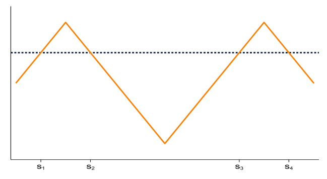
Figure 8: Measure of Underqualification

Figure 8 illustrates a layer given a measure of underqualification $H$ (solid orange line). Layering breaks the original assignment problem into independent problems for each layer, such as the layer indicated by the blue dashed line. Since the number of workers and jobs in between an optimally paired worker $x$ and job $z$ is identical, only workers and jobs within the same layer can be paired. That is, only workers $(s_{1},s_{3})$ and jobs $(s_{3},s_{4})$ can optimally be paired.

3.3 Sorting Within a Layer

We now construct a recursive characterization for an optimal assignment within a given layer. This recursive formulation reflects on the salient features of optimal sorting stemming from concavity of the cost. We use the approach of Aggarwal:1995 that centers on the property of no intersecting pairs. Specifically, we adopt the recursive algorithm developed by Nechaev:2013, designed to model statistical properties of polymer chains.

The optimal assignment problem for a given layer is an alternating assignment problem. An optimal assignment within a layer matches one worker with precisely one job. For notational convenience, we order workers and jobs within each layer by their skill levels. Let there be $n_{\ell}$ workers and $n_{\ell}$ jobs in a given layer, and we denote the skill levels by $s_{1}<s_{2}<\dots<s_{2n_{\ell}-1}<s_{2n_{\ell}}$.

We write a Bellman equation to calculate the minimum aggregate cost of mismatch. The recursive component of the Bellman equation is that we consider assignment problems with an increasing number of skill levels. We start by solving all assignment problems between two consecutive elements: the assignment problem between one worker and one job. That is, we consider assignments between skill levels $s_{i}$ and $s_{i+1}$, for each $i$. Using the solutions from the previous step, we proceed to solve all assignment problems between four consecutive elements (two workers and two jobs) and so on.

We denote by $V_{i,j}$ the minimum cost of mismatch when sorting all workers and jobs with skill levels between $s_{i}$ and $s_{j}$ (inclusive), where $j>i$. The difference $j-i$ is odd so that there are equal numbers of workers and jobs between $s_{i}$ and $s_{j}$. Considering an assignment of workers and jobs with skill levels in $[s_{i},s_{j}]$, the planner can pair the leftmost $s_{i}$ with any $s_{k}$ such that $k-i$ is odd. Upon pairing $s_{i}$ with $s_{k}$, the planner remains to optimally pair the workers and jobs in $[s_{i+1},s_{k-1}]$, and all workers and jobs with skill levels in $[s_{k+1},s_{j}]$. The main observation that facilitates this characterization is that there are no pairings between these two segments because this violates the property of no intersecting pairs. Using the results from previous steps to obtain costs $V_{i+1,k-1}$ and $V_{k+1,j}$ delivers the Bellman equation:

$$V_{i,j}=\min_{k\in\{i+1,i+3,\dots,j\}}\;\big{(}c(s_{i},s_{k})+V_{i+1,k-1}+V_{k+1,j}\big{)}$$ (10)

with boundary conditions $V_{i+1,i}=0$ for all $i$.

Figure 9: Bellman Equation

Figure 9 illustrates the Bellman equation for an optimal sorting. Consider an assignment problem between workers and jobs with skill levels in $[s_{i},s_{j}]$. We can pair the leftmost skill $s_{i}$ with any skill $s_{k}$ such that $k-i$ is odd, as illustrated by the pair $(s_{i},s_{k})$. Upon pairing $s_{i}$ with $s_{k}$, the planner remains to optimally pair the other workers and jobs in $[s_{i+1},s_{k-1}]$, and all workers and jobs with skill levels in $[s_{k+1},s_{j}]$. There are no pairings between these two segments because this violates the property of no intersecting pairs.

Finally, we construct an optimal assignment. Starting from $V_{1,2n_{\ell}}$, the optimal pairing of skill $s_{1}$ is given by skill $s_{k}$ that solves equation (10). Then two corresponding continuation values, $V_{2,k-1}$ and $V_{k+1,2n_{\ell}}$, are evaluated to determine optimal pairings for skill $s_{2}$ and for skill $s_{k+1}$, respectively. This process of finding an optimal assignment continues until a full assignment is constructed.

3.4 Characterizing Optimal Sorting

The three-step approach to characterizing the optimal sorting is as follows. First, we maximize perfect pairs. This leads to positive sorting between identical workers and jobs and we can withdraw them from further analysis. Second, we construct a measure of underqualification to decompose the assignment problem into a sequence of independent layers with $n_{\ell}$ skills in each layer $\ell$. Third, we characterize an optimal assignment for each layer using the Bellman algorithm. The optimal assignment is then given by the following theorem.

Theorem 1.

An optimal assignment between workers $F$ and jobs $G$ sums optimal assignments for each layer, where an optimal assignment in each layer attains $V_{1,2n_{\ell}}$ in the Bellman equation (10).

3.5 Comparative Statics

We next show that optimal sorting becomes more positive, by which we formally mean larger in a natural ordering on assignments called concordance order, as the mismatch cost function becomes less concave. Moreover, we show that there exists a threshold in concavity of costs $\zeta_{p}$ and $\zeta_{u}$ beyond which the optimal assignment within each layer is positive.

For any two assignments $\pi$ and $\hat{\pi}$ between a fixed pair of distributions of workers and jobs, we say that assignment $\pi$ is smaller in concordance order than $\hat{\pi}$, which we denote by $\pi\preceq\hat{\pi}$, if for any coordinate $(x_{c},z_{c})$, less mass is concentrated in both the top-right and bottom-left quadrants under assignment $\pi$ than under $\hat{\pi}$. Intuitively, a more positive sorting corresponds to an assignment larger in concordance order, and this equivalence was made precise by Tchen:1980. When assignment $\hat{\pi}$ is larger in concordance order, it is implied that other measures of statistical association, such as the correlation coefficient, the rank correlation, and Kendall’s $\tau$ coefficient are also larger for $\hat{\pi}$ than for assignment $\pi$ (Joe:1997).

Theorem 2 shows that optimal sorting is more positive when the costs of mismatch becomes less concave, which we prove in Appendix LABEL:a:cs.

Theorem 2.

Suppose the mismatch cost $c(x,z)$ is of the form (5) and that for some increasing convex function $\kappa$, $\hat{c}=\kappa(c)$ is also of the form (5). If $\pi$ is an optimal assignment with costs $c$, then there exists an optimal assignment $\hat{\pi}$ with the less concave mismatch cost $\hat{c}$ such that $\pi\preceq\hat{\pi}$.

Figure 10: Improving the Assignment When Costs of Mismatch Become Less Concave

Figure 10 visualizes an optimal assignment that is no longer optimal when the costs of mismatch become less concave. In this case, there exists a pair $(x_{0},z_{0})$ with positively sorted subpairs $\{(x_{i},z_{i})\}_{i=1}^{p}$, which we display in the top panel, such that the assignment with workers and jobs $\{(x_{i},z_{i})\}_{i=0}^{p}$ can be improved in a more positive fashion, as shown in the bottom panel.