Enhanced entanglement and controlling quantum steering in a Laguerre-Gaussian cavity optomechanical system with two rotating mirrors

Abstract

Gaussian quantum steering is a type of quantum correlation in which two entangled states exhibit asymmetry. We present an efficient theoretical scheme for controlling quantum steering and enhancing entanglement in a Laguerre-Gaussian (LG) rotating cavity optomechanical system with an optical parametric amplifier (OPA) driven by coherent light. The numerical simulation results show that manipulating system parameters such as parametric gain $\chi$, parametric phase $\theta$, and rotating mirror frequency, among others, significantly improves mirror-mirror and mirror-cavity entanglement. In addition to bipartite entanglement, we achieve mirror-cavity-mirror tripartite entanglement. Another intriguing discovery is the control of quantum steering, for which we obtained several results by investigating it for various system parameters. We show that the steering directivity is primarily determined by the frequency of two rotating mirrors. Furthermore, for two rotating mirrors, quantum steering is found to be asymmetric both one-way and two-way. As a result, we can assert that the current proposal may help in the understanding of non-local correlations and entanglement verification tasks.

I Introduction

Quantum entanglement is one of the most weirdest phenomenon of quantum mechanics in which there exists a non-classical (non-local) correlation between spatially separated states ent ; ent1 . Entanglement has been shown to have numerous applications in quantum information processing tele ; ram , quantum teleportation tele ; ram , quantum algorithms algo , and quantum computing ent2 ; comp . In recent years, many of the theoretical and experimental studies focused on the generation of microscopic entanglement in systems such as atoms, ions, and photons micro ; micro1 ; micro2 . However, it remained a pipe dream for researchers to generate quantum entanglement for macroscopic objects. As a result of hard efforts, macroscopic entanglement has been experimetally demonstrated for superconducting qubits sup , atomic ensembles atom and entanglement between diamonds diam .

In addition to quantum entanglement, Einstein-Podolsky-Rosen (EPR) steering epr is one of an important quantum correlation that sits between Bell’s non-locality and entanglement bell ; bell1 ; bell2 . As there exists non-exchangeable asymmetric roles between the two observers, Alice and Bob. This phenomenon was first introduced by Schrödinger to show that the non-locality in EPR states sch ; sch1 . Most distinctive and unique feature of quantum steering is its directionality dir . It is interesting to mention here that the steerable states of massive and macroscopic objects can be utilized to test the foundational issues of quantum mechanics and the implementation of quantum information processing. In recent years, many of the studies has focused to achieve these goals in many optomechanical stee ; stee1 ; stee2 and in magnomechanical systems opent3 ; opent4 ; opent5 . It is because of advancement in present day technology that the most promising feature of quantum steering, one-way steering, has been experimentally demonstrated exp ; exp1 .

Over the course of about last two decade, cavity optomechanical systems oms ; oms2 ; oms3 have gained importance due to its academic significance and applications in foundational issues of quantum mechanics found and highly precise measurements measure . Optomechanical systems have recently sparked widespread interest in their discussion of quantumness wig1 via the Wigner function naeem1 ; naeem2 and time-frequency analysis naeem3 . In addition to above, optomechanical systems have been experimentally used because of the development of optical micro-cavity technology. They provide an excellent test bed macroscopic entangled state opent ; opent1 ; opent2 , coherent state SigJS ; coh , squeezed state sq ; Sin , ground state cooling cool and optomechanically induced transparency (OMIT) omit ; omit1 ; omit2 ; Sn1 ; Sn2 . In principle, nothing from the principles of quantum mechanics prohibit macroscopic entanglement. This has been first investigated by Vitali and collaborators in their seminal paper oms . Therefore, optomechanics is paving a way towards the macroscopic non-local correlations at macroscopic scales.

Motivated by the progress in optmechanical systems, Bhattacharya and Meystre proposed an optomechanical system comprising a rotating mirror (or rovibrational mirror) which is directly coupled to a Laguerre-Gaussian (LG) cavity mode via exchange of angular momentum bhatt ; bht . In their scheme, they demonstrate that the rotating mirror can be sufficiently cooled to 8mK right from the room temperature (300K), due to the incident radiation torque. At such low temperature, one can observe various nonlinear and quantum phenomena. In another interesting scheme, Bhattacharya and collaborators, showed that one can generate entanglement between mechanical rotating mirror and LG cavity mode bhatt1 . More recently, researchers found that orbital angular momentum of LG cavity mode can be measured by utilizing OMIT window width peng ; XHYM . Furthermore, researcher used hybrid rotational system to study OMIT QingL ; peng3 ; YXW ; ZAAK ; Rao , cooling of rotating mirrors QioP , and entanglement peng1 ; peng2 ; Singh ; FWK . Most recently, there is an interesting study by Huang et al, in which they proposed a LG cavity optomechanical scheme, assisted with an optical parametric amplifier (OPA) whose pump frequency is double the frequency of frequency of anti-Stokes field which is being generated by the external laser beam interacting with both rotating mirrors, for exploring the entanglement between two rotating mechanical mirrors huang and showed that the maximum entanglement is restricted by the gain of the OPA.

The current research focuses on the controllable quantum steering and enhanced entanglement in a resolved-side-band of two rotating mechanical mirrors of a single LG optomechanical cavity containing an OPA. We specifically investigated mirror entanglement as well as quantum steering of rotating mirrors, and our results show that parametric interactions have increased entanglement. Moreover, we also discussed the dependence of entanglement upon several system parameters such as parametric gain $\chi$, effective detuning $\Delta$ and parametric phase $\theta$. It is also shown that there exists tripartitite (mirror-cavity-mirror) entanglement, quantified by residual cotangle. In addition to entanglement, we also studied the control of quantum steering $\xi$, which has been found to be asymmetric both one-way and two-way for rotating mirrors RM₁ and RM₂, respectively.

The paper is arranged as follows. In Section 2, we present the theoretical model and the corresponding dynamical quantum langevin equations. The discussion of methodology for measuring entanglement and quantum steering is covered in Section 3. We present numerical results that discuss bipartite/tripartite entanglement and quantum steering in Section 4 and Section 5, respectively, then Section 6, shows the experimental feasibility of the present scheme. Finally, Section 7 presents the conclusions.

II Theoretical Model

The system we considered comprises an optical cavity with length $L$ with two rotating mirrors, as shown in Figure 1. The cavity is driven by the input Gaussian beam which has no topological charges. The Gaussian beam with frequency $\omega_{L}$ and zero charge enters the cavity through the left rotating mirror (RM₁), which is partly transmissive. The reflected beam gets a charge $-2l$ while the transmitted beam obtain zero charge. Moreover, the transmitted beam is then incident on the right rotating mirror (RM₂) and gets charge $2l$ (zero) on reflection (transmission) from RM₂. Thus a beam with charge $2l$ interacts with the RM₁ again. The transmitted beam from RM₁ has charge $2l$ while the reflected beam remains with no charge, demonstrating that the net topological charge increment of light transmission back and forth in the cavity is zero, ensuring the stability of the system. Moreover, the coupling between the cavity and left/right rotating mirrors established due to the exchange of orbital angular momentum. Therefore, we can expect the entanglement between two rotating mirrors. The exchange of angular momentum between each rotating mirror and each intracavity photon is $2l\hbar$ and time for a round trip is $2L/c$, thus the radiation torque acting on both mirror is the change in angular momentum per the time required for a round trip, that is, $\frac{2l\hbar}{(2L/c)}=\frac{cl\hbar}{L}=\hbar g_{\phi}$, where $g_{\phi}=cl/L$ optorotational coupling strength. For simplicity, we assumed the same radius $R$ and the same mass $m$, and the same intrinsic damping rate $\gamma_{m}$. In addition, a degenerate OPA is embedded into the cavity. Finally, the beam is completely reflected from RM₂. Moreover, we have ignored the loss of incident light ASRA . In a frame rotating at the driving frequency $\omega_{L}$, the Hamiltonian of the whole system takes the form

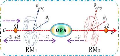
Figure 1: Diagrammatic scheme consists of two rotating mirrors RM₁ and RM₂ coupled to the Laguerre-Gaussian cavity mode via exchange of angular momentum. The two rotating mirrors are mounted on support S1 and S2, respectively and have the same direction along the cavity axis $z$. The angular deflections of the two rotating mirror are denoted by the angle which are taken from their equilibrium position. In addition, a degenrate OPA is embedded inside the LG-cavity and pumped by a coherent light.

$$H/\hbar = \left[\Delta_{0}+(g_{1}\varphi_{1}-g_{2}\varphi_{2})\right]a^{\dagger}a+\frac{1}{2}\sum_{j}^{2}\omega_{\varphi_{i}}\left(L_{z_{i}}^{2}+\varphi_{i}^{2}\right)$$ (1)

$$+i\chi(a^{{\dagger}^{2}}e^{i\theta}-a^{2}e^{-i\theta})+\iota E\left(a^{\dagger}-a\right),$$

where $\Delta_{0}=\omega_{c}-\omega_{L}$ is the detuning of the cavity field and $a$ ($a^{\dagger}$) is the annihilation (creation) operator of the cavity field, and follow the relation $\left[a,a^{\dagger}\right]=1$. While $\phi_{j}$ and $L_{z_{k}}$ are the angular displacement and angular momentum of the rotating mirrors, respectively, with $[\phi_{j},L_{z_{k}}]=i\delta_{jk}(j,k=1,2)$. In above Hamiltonian, the first two terms are the bare Hamiltonian of the energy for the cavity field and the two rotating mirrors, the third term describes the optomechanical coupling between the cavity field and the two rotating mirrors with the coupling constant given by $g_{i}=(cl/L)\sqrt{\hbar/I\omega_{\phi_{i}}}\left(i=1,2\right)$ 11 , where $c$ is the velocity of light and $l$ is the orbital angular momentum quantum number, $L$ is the length of the cavity and $I=MR^{2}/2$ is the moment of inertia of the two rotating mirrors about the central axis of the cavity. The next term interprets the interaction of the 2nd-order nonlinear optical crystals, at $2\omega_{L}$, with the L-G cavity mode with $\chi$ ($\theta$) being the parametric gain (phase) of the OPAs. The last term of Equation (1) represents the interaction of the LG-cavity mode with the incoming coupling field.

The dynamics of the system can be well described by the time evolution of the operators and is given by the quantum Langevin equations (QLEs), which can be written as:

$$\dot{\phi}_{j} = \omega_{\phi_{j}}L_{z_{j}},(j=1,2)$$ (2a)

$$\dot{L}_{z_{j}} = -\omega_{\phi_{j}}\phi_{j}+g_{\alpha j}a^{\dagger}a-\gamma_{m}L_{z_{j}}+\varepsilon^{in},$$ (2b)

$$\dot{a} = -[\kappa+i{\Delta_{\circ}+(g_{1}\phi_{1}-g_{2}\phi_{2})}]a+2\chi a^{{\dagger}}e^{i\theta}$$ (2c)

$$+E+\sqrt{2\kappa}a^{in},$$

where $$g_{\alpha{1}}=-g_{1} g_{\alpha{2}}=g_{2} \Delta_{\circ}=\omega_{c}-\omega_{L} \varepsilon^{in} T$$, and . In addition, account for the mechanical noise, and its fluctuation correlations which are relevant to temperature , can be described by

$$\left\langle\delta\varepsilon^{in}(t)\delta\varepsilon^{in}(t^{{}^{\prime}})\right\rangle=\frac{\gamma_{m_{i}}}{\omega_{\phi_{i}}}\int\limits_{-\infty}^{\infty}\frac{d\omega}{2\pi}e^{-\iota\omega(t-t^{{}^{\prime}})}\omega\left[1+\Theta\right],$$ (3)

where $\Theta=\coth\left(\frac{\hbar\omega}{2k_{B}T}\right)$, with $k_{B}$ being the Boltzmann’s constant. Similarly, $a^{in}$ is a noise operator that of the incident laser beam on the optical cavity and whose delta-correlated fluctuations are

$$\left\langle a^{in}(t)a^{in,\dagger}(t)\right\rangle=\delta(t-t^{{}^{\prime}}),$$ (4)

To linearize the set of QLEs, i.e., Equation (2a-2c), we use the ansatz by writing $\tau=\tau_{0}+\delta\tau$, $(\tau=\phi_{j},L_{z_{j}},a)$, where $\tau_{s}$ ($\delta\tau$) is the steady-state (quantum fluctuation ) of the operators. Under the long-term limit, the steady-state values of each operator are:

$$L_{z_{j}} = 0,$$ (5a)

$$\phi_{j0} = \frac{g_{\alpha{j}}\left|a_{0}\right|^{2}}{\omega_{\phi_{1}}},$$ (5b)

$$a_{0} = \frac{(\kappa-i\Delta+2\chi e^{i\theta})}{(\kappa^{2}+\Delta^{2}+4\chi^{2})}E,$$ (5c)

where $$\Delta=\Delta_{0}+\sum_{j}^{2}g_{j}\phi_{j0} a_{0} |a_{s}|\gg\delta a \delta a\delta a^{\dagger}$$ represents the effective cavity detuning while denotes the effective field amplitude of cavity modified by OPA. Since, , one can omit the unwanted nonlinear terms, e.g., . In this case, the linearized set of QLEs takes the form:

$$\delta\dot{\phi}_{j} = \omega_{\phi_{j}}\delta L_{z_{j}},$$ (6a)

$$\delta\dot{L}_{z_{j}} = -\omega_{\varphi_{j}}\delta\phi_{j}-\gamma_{m}\delta L_{z_{j}}+G_{j}\delta X+\delta\varepsilon^{in},$$ (6b)

$$\delta\dot{X} = -\kappa\delta X+\Delta\delta Y+\sqrt{2\kappa}X^{in},$$ (6c)

$$\delta\dot{Y} = -\kappa\delta Y-\Delta\delta X-G_{1}\delta\phi_{1}+G_{2}\delta\phi_{2}$$ (6d)

$$+\sqrt{2\kappa}Y^{in},$$

where $$G_{j}=\sqrt{2}g_{\alpha j}a_{0} \delta X=\frac{1}{\sqrt{2}}(\delta a+\delta a^{{\dagger}}) \delta Y=\frac{1}{\sqrt{2}i}(\delta a-\delta a^{{\dagger}}) \delta X_{in}=\frac{1}{\sqrt{2}}(\delta a_{in}+\delta a_{in}^{{\dagger}}) \delta Y_{in}=\frac{1}{\sqrt{2}i}(\delta a_{in}-\delta a_{in}^{{\dagger}})$$ is the effective optomechanical coupling strength. Here, we have introduced the set of quadratures for the cavity field, that is, , , and . Hence, we rewrite the QLEs (Equation (6a-6d)) in a more compact form, as follow

$$\mathcal{\dot{Z}}(t)=\mathcal{A}\mathcal{Z}(t)+n(t),$$ (7)

where $\mathcal{Z}^{T}=(\delta\phi_{1},\delta L_{z_{1}},\delta\phi_{2},\delta L_{z_{2}},\delta X,\delta Y)$ is the fluctuation vector and $n^{T}(t)=(0,\varepsilon^{in},0,\varepsilon^{in},\sqrt{2\kappa}X^{in},\sqrt{2\kappa}Y^{in})$ represents the noise vector. Therefore, the drift matrix of the system is given by

$$\mathcal{A}=\left(\begin{array}[]{cccccc}0&\omega_{\phi_{1}}&0&0&0&0\\ -\omega_{\phi_{1}}&-\gamma_{m}&0&0&-G_{1}&0\\ 0&0&0&\omega_{\phi_{2}}&0&0\\ 0&0&-\omega_{\phi_{2}}&-\gamma_{m}&G_{2}&0\\ 0&0&0&0&\mu_{+}&\rho_{+}\\ -G_{1}&0&G_{2}&0&\rho_{-}&\mu_{-}\end{array}\right),$$ (8)

where $\mu_{\pm}=-\kappa\pm 2\chi\Re(e^{\theta})$ and $\rho_{\pm}=\pm\Delta+\Im(e^{\theta})$. The above drift matrix of the system determines the stability of the optorotational system, is stable and reaches its steady-state if none of the eigenvalues of the above drift matrix $\mathcal{A}$ has a positive real part RHC .

III Entanglement and Gaussina Steering measurement

Covariance Matrix. The foremost task is to find the stability of any system which, in this case, is obtained by applying the Routh-Hurwitz criterion which impose certain constraints on the system parameters. Once the constraints for the current optorotational system are fulfilled, the steady state of the fluctuations must be a Gaussian state. Since, $\langle\varepsilon^{in}\rangle=\langle a^{in}\rangle=0$, and in this situation, quantum correlations of the system can then be characterized by the covariance matrix, which has the same order as the drift matrix, with $V_{jk}=[\mathcal{Z}_{j}(\infty)\mathcal{Z}_{k}(\infty)+\mathcal{Z}_{k}(\infty)\mathcal{Z}_{j}(\infty)]/2$, where

$$\mathcal{Z}^{T}(\infty) = (\delta\phi_{1}(\infty),\delta L_{z1}(\infty),\delta\phi_{2}(\infty),\delta L_{z2}(\infty),$$ (9)

$$\delta X(\infty),\delta Y(\infty))$$

represents the fluctuation matrix. The elements of the covariance matrix take the form CWSP

$$V_{jk}=\sum_{k,l}\int_{0}^{\infty}dt\int_{0}^{\infty}dt^{\prime}\Lambda_{i,k}(t)\Lambda_{j,l}(t^{\prime})\Psi_{k,l}(t-t^{\prime}),$$ (10)

where $\Lambda=\text{exp}(\mathcal{A}t)$ and

$$\Psi_{k,l}(t-t^{\prime})=\langle n_{k}(t)n_{l}(t^{\prime})n_{l}(t^{\prime})n_{k}(t)/2$$ (11)

is noise correlation functions matrix. For large mechanical quality factor, the quantum Brownian noise can be delta-correlated, that is

$$\Psi_{k,l}(t-t^{\prime}) = D_{k,l}\delta(t-t^{\prime}),$$

$$= \text{Diag}[0,\gamma_{m_{1}}(2n_{1}+1),0,\gamma_{m_{1}}(2n_{2}+1),\kappa,\kappa],$$

which simplifies Equation (10) as follow

$$V=\int_{0}^{\infty}dt\Lambda(t)D\Lambda^{T}(t).$$ (12)

The covariance matrix $V$ of system satisfy steady-state Lypunov equation,

$$\mathcal{A}V+\mathcal{A}V^{T}=-D.$$ (13)

The covariance matrix $V$ which delineate the entanglement configuration of the current two mirrors optorotational system, its form is

$$V=\left(\begin{array}[]{ccc}M_{1}&N_{12}&N_{1m}\\ N_{12}^{T}&M_{2}&N_{2m}\\ N_{1m}^{T}&N_{2m}^{T}&M_{m}\end{array}\right).$$ (14)

Each entry of above covariance matric $V$ is a $2\times 2$ block matrix. The diagonal entries of the above covariance matrix $V$ describe the local properties of the participants while the rest of the entries define the the correlations between different modes.
Bipartite entanglement. The logarithmic energy which quantify the entanglement is defined as

$$E_{N}=\max[0,\ln(2\nu^{-})],$$ (15)

where $\nu^{-}=2^{-\frac{1}{2}}\sqrt{\aleph-\sqrt{\aleph^{2}-4\det\varsigma}}$ is the smallest symplectic eigenvalue of the partially transposed covariance matrix (CM), $\varsigma=[\varsigma_{\alpha},\ \varsigma_{\alpha\beta};\varsigma_{\alpha\beta}^{T},\varsigma_{\beta}]$ with each entry of the $\varsigma$ is a $2\times 2$ block matrix and therefore, $\varsigma$ is the $4\times 4$ CM of the bipartite subsystem involving mode $\alpha$ and $\beta$ and $\aleph=\det\varsigma_{\alpha}+\det\varsigma_{\beta}-2\det\varsigma_{\alpha\beta}$.

Tripartite entanglement. We opt the minimum residual cotangle Adesso ; Adesso2 ; Coffman for the basic criteria to realize tripartite entanglement, is given by

$$\mathcal{R}_{\tau}^{min}\equiv\min[\mathcal{R}_{\tau}^{m_{1}|m_{2}a},\mathcal{R}_{\tau}^{m_{2}|m_{1}a},\mathcal{R}_{\tau}^{a|m_{1}m_{2}}],$$ (16)

where $\mathcal{R}_{\tau}^{f|jk}\equiv C_{f|jk}-C_{f|j}-C_{f|k}\geq 0$ ($f,j,k=m_{1},m_{2},a$) is the monogamy of quantum entanglement and this condition assures the invariance of tripartite entanglement under possible permutations of all modes. Hence, $\mathcal{R}_{\tau}^{min}$ and is describes the genuine tripartite entanglement of any three-mode Gaussian state. In Equation (16), $C_{f|j}$ is the contangle of subsystems of $f$ and $j$ ( $j$ incorporate one or two modes), and is equal to the squared logarithmic negativity. To execute one-mode-vs-two-modes logarithmic negativity $E_{f|jk}$, one must reform $\nu^{-}$ (see Equation (15)) as

$$\nu^{-}=\min eig\ |\bigoplus_{j=1}^{3}(-\sigma_{y})\widetilde{V_{4}}|,$$ (17)

where $\widetilde{V_{4}}=\mathcal{P}_{1|2}\mathcal{V}_{4}\mathcal{P}_{1|2}$ with $\widetilde{\mathcal{Q}}=\mathcal{G}_{i|jk}\mathcal{Q}\mathcal{G}_{i|jk}$. Furthermore Furthermore, the partial transposition matrices are given by

$$\mathcal{G}_{1|23} = \text{diag}(1,-1,1,1,1,1),$$

$$\mathcal{G}_{2|13} = \text{diag}(1,1,1,-1,1,1),$$

$$\mathcal{G}_{3|12} = \text{diag}(1,1,1,1,1,-1).$$

Parameters	Symbol	Value
Length of the cavity	$L$	$1$mm
Mass of rotating mirrors	$m$	$35$ng
Radius of rotating mirrors	$R$	$10\mu$m
Left mirror angular frequency	$\omega_{\phi_{1}}/2\pi$	$10^{7}$Hz
Right mirror angular frequency	$\omega_{\phi_{2}}$	$(0.5-1.5)\omega_{\phi_{1}}$
Input laser power	$\wp$	$50$mW
Quality factor	$Q$	$2\times 10^{7}$
Laser wavelength	$\lambda$	$810nm$
Optical finesse	$F$	$5\times 10^{3}$
Orbital angular momentum	$l$	$100\hbar$
Temperature	T	15 mK

Table 1: Experimental values of the parameters used in the paper bhatt ; bhatt1 ; peng1

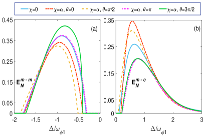
Figure 2: (a) The mirror-mirror entanglement $E_{N}^{m-m}$ and (b) the mirror-cavity entanglement $E_{N}^{m-c}$ plotted as a function of the normalized detuning $\Delta/\omega_{\phi 1}$.

Gaussian steering. Gaussian steering has asymmetric characteristics in nature and is much different from the entanglement. For the two interacting mode Gaussian state, the recommended measurements of the quantum steerability between any two interacting parties in different directions can be calculated as

$$\zeta_{\alpha|\beta} = \max\{0,\mathcal{S}(2\mathcal{V}_{m_{l}})-\mathcal{S}(2\mathcal{V}_{in})\},$$ (18a)

$$\zeta_{\beta|\alpha} = \max\{0,\mathcal{S}(2\mathcal{V}_{m_{2}})-\mathcal{S}(2\mathcal{V}_{in})\},$$ (18b)

where $$\mathcal{S}(\nu) \mathcal{S}(\nu)=\frac{1}{2}\ln\det(\nu)$$ is the Rényi-2 entropy and is , and

$$\mathcal{V}_{in}=\left[\begin{array}[]{cc}\mathcal{V}_{m_{1}}&\mathcal{V}_{m_{1}m_{2}}\\ \mathcal{V}_{m_{1}m_{2}}^{T}&\mathcal{V}_{m_{2}}\end{array}\right],$$ (19)

The diagonal entries of $\mathcal{V}_{m_{1}}$ and $\mathcal{V}_{m_{2}}$ defines the reduced states of modes $\mathcal{V}_{m_{1}}$ and $\mathcal{V}_{m_{2}}$, respectively. We quantify the quantum steering by $\zeta_{\alpha|\beta}$ which translates the mode $\alpha$ steers mode $\beta$ and similarly $\zeta_{\beta|\alpha}$ defines the swaped direction. It is an established fact that the entanglement is symmetric property. However, the EPR steering is intrinsically different from entanglement, i.e., asymmetric property which means that a quantum state may be steerable from Bob to Alice but not vice versa. Therefore, there exist mainly three different possibilities for quantum steering. (i) $\zeta_{\alpha|\beta}=\zeta_{\beta|\alpha}=0$ as no-way (NW) steering, (ii) $\zeta_{\alpha|\beta}>0$ and $\zeta_{\beta|\alpha}=0$ or $\zeta_{\alpha|\beta}=0$ $\zeta_{\beta|\alpha}>0$ as one-way (OW) steering and $\zeta_{\alpha|\beta}>0$ $\zeta_{\beta|\alpha}>0$ as two-way (TW) steering. Asymmetric steerability between the two modes of the Gaussian states can be checked by introducing the steering asymmetry, defined as

$$\zeta_{M}=|\zeta_{\alpha|\beta}-\zeta_{\beta|\alpha}|.$$ (20)

It is vital to mentioned here that we obtain one-way or two way steering as long as steering asymmetry remains positive, i.e., $\zeta_{M}>0$ and no-way if $\zeta_{M}=0$.

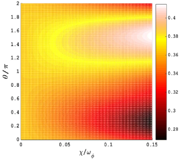
Figure 3: (Color Online) Density plot of (a) the mirror-mirror entanglement $E_{N}^{m-m}$ versus $\chi$ and $\phi$.

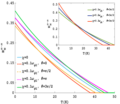
Figure 4: The logarithmic negativity $E_{N}^{m-m}$ as a function of temperature in the absence and presence of the OPA with optimum detuning.

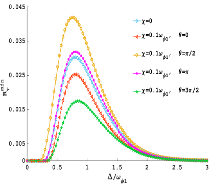
Figure 5: Genuine tripartite entanglement (mirror-cavity-mirror) versus the normalized detuning. The parameters are same as given in Table.

IV Bipartite and Tripartite Entanglement

In the following discussion, we demonstrate the results regarding the generation of bipartite (and tripartite) entanglement and quantum steering for the current system. Throughout our numerics, we have assumed experimentally realizable parameters, similar to those in ref bhatt ; bhatt1 ; peng1 , listed in Table 1. In this paper, we consider two bi-partitions, namely $E_{N}^{m-m}$ and $E_{N}^{m-c}$ to represent the degree of entanglement between two phonon modes and between L–G cavity mode and phonon mode, respectively. The utmost task of studying the entanglement in such a double rotational cavity optomechanical system is to find optimal value of the cavity detuning $\Delta$. In Figure 2 (a-b), the logarithmic negativity is plotted as a function of the detuning in the absence and presence of parametric gain (with different parametric phases). To ensure the stability of the system, we choose the parameter gain $\chi=0.1\omega_{\phi_{1}}$. We find that the steady state entanglement between two mirrors $E_{n}^{m-m}$ (between the mirror and the cavity $E_{n}^{m-c}$) is obtained when $\Delta<0$ ($\Delta>0$) in the steady state which is similar to bhatt1 ; peng1 . In addition, the maximal value of $E_{n}^{m-m}$ ($E_{n}^{m-c}$) is obtained at about $\Delta=-\omega_{\phi_{1}}$ ($\Delta=\omega_{\phi_{1}}$). Furthermore, the enhancement pattern of entanglement $E_{n}^{m-m}$, by varying the phase of the parametric, behaves almost in converse manner as compared to $E_{n}^{m-c}$ as shown by Figure 2 (a-b).

Next, we examine the combined effect of parametric gain and parametric phase (associated with the gain), on the mirror-mirror entanglement $E_{n}^{m-m}$ and mirror-cavity entanglement $E_{n}^{m-c}$ as shown by the Figure 3. Physically, the gradual increase of parametric gain induces the nonlinearity in the system and consequently, we observe the enhancement in entanglement. One can see that bipartite entanglement $E_{n}^{m-m}$ increases as the $\theta$ increases for a larger value of parametric gain. We can also see from the Figure 3 that by ensuring the stability of the current system, the maximum enhancement of $E_{n}^{m-m}$ appears around $\theta=3\pi/2$ for varied parametric gain. For specific value of $\chi$, the amount of maximum entanglement increase, is different. For example, keeping the fixed parametric gain, i.e., $\chi=0.1\omega_{\phi_{1}}$, the amount of maximum entanglement $E_{n}^{m-m}$ increased, is about $14\%$.

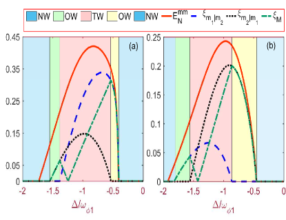
Figure 6: Plot of the mirror-mirror entanglement $E_{N}^{m-m}$ (solid orange line), Gaussian steering $\zeta_{m_{1}|m_{2}}$ (dashed blue line), $\zeta_{m_{2}|m_{1}}$ (dotted black line) and the steering asymmetry $\zeta_{M}$ (dot-dashed green line) of the two rotational modes as a function of the normalized detuning $\Delta/\omega_{\phi 1}$ when (a) $\omega_{2}=0.5\omega_{1}$ and (b) $\omega_{2}=1.5\omega_{1}$. We set $\chi=0$. The rest of the parameters are same as in Table. 1.

The robustness of such a mirror-mirror entanglement in two rotating cavity optomechanical system with respect to the temperature $T$ as shown in Figure 4. It is clear that for a fixed value of the parametric gain, the amount of entanglement decreases monotonically as the temperature of the environment increases. and eventually cease to exist. However, the critical temperature of mirror-mirror entanglement fluctuate by varying the parametric phase. On the other hand, the curve shown in the inset of Figure 4 have dissimilar tendency i.e., by choosing the optimal value of the parametric phase, the degree of mirror-mirror entanglement $E_{n}^{m-m}$ increases with the rise of parametric gain. However, the temperature decreases, implying that the system with larger parametric gain mass possess weaker capability to refrain from decoherence of the thermal environment.

One of the most vital contribution in the present double rotating system is to find the possibility of exploring the genuine tripartite entanglement. In Figure 5, we investigate the genuine tripartite entanglement versus normalized detuning. It is clear that the genuine tripartite entanglement among the participants (i.e., phonon-photon-phonon) exists in the current double rotating system if the cavity mode is in blue sideband. The solid blue curve shows the genuine tripartite entanglement when $\chi=0$. However, in the presence of parametric gain $\chi=0.1\omega_{\phi_{1}}$, we plot tripartite entanglement for different value of phase. It is clear from Figure 5 that maximum enhancement in tripartite entanglement is obtained for $\theta=\pi/2$. It is also noticeable that this enhancement go along with an increase in domain of genuine tripartite entanglement over a relatively wider range of effective cavity detuning. Furthermore, the maximum of genuine tripartite entanglement with parametric phase increases by $40\%$. Hence, the parametric phase of the OPA plays a vital role in enhancing the genuine tripartite entanglement as exhibited in Figure 5.

V Controlling Gaussian Steering

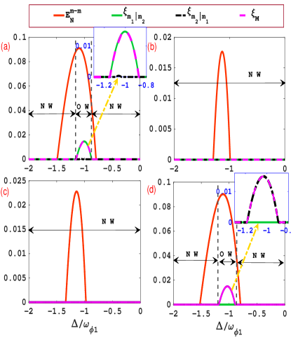
Figure 7: The mirror-mirror entanglement (solid orange line), Gaussian steering $\zeta_{m_{1}|m_{2}}$ (solid green line), $\zeta_{m_{2}|m_{1}}$ (dot-dashed black line) and the steering asymmetry $\zeta_{M}$ (dashed magenta line) as a function of the normalized detuning $\Delta/\omega_{\phi 1}$ when (a) $\omega_{\phi_{2}}=0.9\omega_{\phi_{1}}$, (b) $\omega_{\phi_{2}}=0.95\omega_{\phi_{1}}$, (c) $\omega_{\phi_{2}}=1.05\omega_{\phi_{1}}$ and (d) $\omega_{\phi_{2}}=1.1\omega_{\phi_{1}}$. The rest of the parameters are same as in Fig. 6 and in Table. 1.

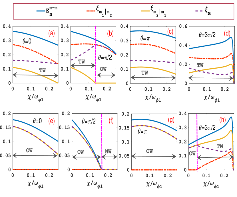
Figure 8: Quantum steering as a function of $\chi/\omega_{\phi 1}$ for different values of $\theta$: (a)-(e) for $\theta=0$, (b)-(f) is for $\theta=\pi/2$, (c)-(g) represents the cases when $\theta=\pi$, and (d)-(h) with $\theta=3\pi/2$. In addition, we set $\omega_{\phi_{2}}=0.5\omega_{\phi_{1}}$ in (a)-(d) and $\omega_{\phi_{2}}=1.5\omega_{\phi_{1}}$ in (e)-(h).We set the optimal value of the detuning. The rest of the parameters are kept same as given in Table. 1.

Two-way (TW) control. In the following, our purpose is to find the controllable quantum steering in the double rotational cavity optomechanical system. Since the entanglement and the quantum steering are two different facets of inseparable quantum correlations, therefore, it is better to study them simultaneously under the same conditions. For this purpose, we employ the Rényi-2 entropy to quantify the steerability between the two rotational modes. We first demonstrate this idea in Figure 6, the peak values of the entanglement and quantum steering of the two mechanical modes. It is evident from Figure 6. that steerable states are always entangled, however, the reverse order is not generally true, i.e., entangled states are not usually steerable. This property reflects the idea that stronger quantum correlations, between the two rotational modes, are indispensable for realizing the Gaussian steering than that for the entanglement. In such a two-rotating cavity optomechanical system, there may exist (one-) two-way quantum steering between the two rotational modes due to frequency difference. To demonstrate the Gaussian steering more clearly, we use the pink area to area to depict the presence of two-way steering, green and yellow areas for one-way steering, and the blue area to represent the presence of no-way steering. It is clear from Figure 6 (a-b), that both the mirror steer each other, however, the steerability mainly depends on the frequency of each mirror. The mirror which has high frequency steers more as compared to the mirror which has less frequency as clearly demonstrated by the pink area in Figure 6 (a-b). The two-way steering implies that both Alice and Bob can convince each other that the state they shared, is entangled. Furthermore, Figure 6. reveal situation where $\zeta_{m_{1}|m_{2}}>0$, $\zeta_{m_{2}|m_{1}}=0$ and $E_{N}^{m-m}>0$ (or $\zeta_{m_{1}|m_{2}}=0$, $\zeta_{m_{2}|m_{1}}>0$ and $E_{N}^{m-m}>0$) witnesses the Gaussian one-way (OW) steering region as shown by the green (yellow) region. One-way (OW) steering in the current system translates that the states of the two rotational modes are steerable in single direction even though they are entangled. Such a kind of response is a direct manifestation of the problem which has been reported in dir . Furthermore, Figure 6 also shows that not only the two steerabilities $\zeta_{m_{1}|m_{2}}$ and $\zeta_{m_{2}|m_{1}}$ but also the entanglement $E_{N}^{m-m}$ are strongly sensitive to the frequencies of the two mechanical modes. Moreover, it can be seen that when the value of the frequency of mirror-2 is greater than the mirror-1, the region for the one-way (two-way) steering gets broaden (shorten).

One-way (OW) control. As we discussed, the steerability and entanglement between the rotational modes are sensitive to their frequencies. We observe that when the two rotational modes are about to synchronize, i.e., the ratio of the frequency of the two rotating mirrors approaches unity, the two-way steering completely vanishes. Furthermore, Figure 7(a) and 7(d) present a fascinating situation where the states of the two rotational modes are entangled; though they show steerability in one direction, which indicates the perfect asymmetry of quantum correlations (one-way steering). Such an asymmetry of quantum correlations describes that both Alice and Bob can execute the same Gaussian measurements on their side of the entangled system, however, they find completely different results. One-way steering can be explained by the steering asymmetry introduced in Eq. (20). Figure 7(a) and 7(d) clearly show that one-way steering can be observe until $\omega_{\phi_{2}}/\omega_{\phi_{1}}=0.9$ or $\omega_{\phi_{2}}/\omega_{\phi_{1}}=1.1$. The one-way steering has been experimentally realized in dir ; exp1 and imparts one-side device independent quantum key distribution (QKD). However, we observe no-way steering when $\omega_{\phi_{2}}/\omega_{\phi_{1}}\simeq 0.95$ or $\omega_{\phi_{2}}/\omega_{\phi_{1}}\simeq 1.05$. Furthermore, when the two rotating mirrors rotate with exactly the same frequency (complectly synchronize), even the entanglement between rotating mirrors completely cease to exist (not shown).

Effect of Parametric Gain and Phase on quantum steering. Finally, the degree of entanglemnt entanglement and dynamics quantum steering can be studied under influence of the parametric gain for different value of phase as shown in Figure 8 around the optimum value of the cavity detuning. Firstly, it can be seen in Figure 8. that quantum steering remains upper bounded by the entanglement irrespective of which rotational mirror has higher frequency. Figure 8 (a-d) shows that with gradual increase of the parametric gain, the two rotational modes exhibit two-way steering except the case when $\theta=\pi/2$, where two-way steering converts to one-way steering around $\chi/\omega_{\phi_{1}}=0.13$. This is because we obtained reduced entanglement at this parametric phase (can be seen in Figure 2(a)). The same situation can also be observe in lower panel of Figure 8, where the one-way steering vanishes around $\chi/\omega_{\phi_{1}}=0.16$. Owing to the gradual enhancement of entanglement for $\theta=3\pi/2$, one-way steering converts to two-way steering for large value of parametric gain. Hence, the current scheme may provide motivation for handling quantum steering in two rotational cavity optomechanical system.

VI Experimental implementations

The parameters for the current scheme is given in Table. 1. Keeping these parameters in mind, we now talk about the feasibility of the current two rotating system based on the recent experiments. In recent experiment, the value of the angular momentum is taken very high because it can easily be realizable via spiral phase elements. In addition, the azimuthal structure of beam of light can be altered via transmission or reflection from the spiral phase elements SYC . It is shown that low mass of the rotational mirrors with high precision can be well fabricated. Futhermore, topological charge of the LG laser beams can be taken as high as $1000$ SYC . With the fast growing nanotechnology, the mechanical oscillators, with low effective mass ($m=37pg$), high-quality factor ($Q_{m}=10^{8}$) and and high frequency (a few MHz), has been experimentally reported KHG . This implies that the current system is an experimentally feasible system under the present-day technology.

VII Conclusions

We have presented an efficient and effective method for improving the entanglement and one-way (two-way) steering characteristics of two rotating mirrors in a Laguerre-Gaussian (LG) rotating cavity, which composed of two rotational mirrors coupled to a cavity via orbital angular momentum exchange and an optical parametric amplifier (OPA) driven by coherent light. We have shown that the frequencies of two rotational mirrors play a vital role in modulating the entanglement and controlling the quantum steering. For example, when $\omega_{\phi 2}=0.5\omega_{\phi 1}$ ($\omega_{\phi 2}=1.5\omega_{\phi 1}$), the steerability of two mirrors is enhanced as compared to the case when the two mirrors are near to synchronized, that is, near the resonance frequency, two-way steering converts to one-way steering (or no-way steering) with a reduced degree of entanglement. It is interesting to mention that the switch from two-way steering to one-way (or no-way) steering is practicable by changing the frequencies of two rotational mirrors, parametric gain and phase. Hence, we argued that the steering directivity in the current scheme would support understanding the quantum correlation and may have major applications in one-way (two-way) quantum computing, quantum secret sharing, and quantum key distribution.

Data availability

All numerical data that support the findings in this study is available within the article

References

- (1) E. Schrodinger, Proc. Cambridge Philos. Soc. 1935, 31(4), 555.
- (2) R. Horodecki, P. Horodecki, M. Horodecki, K. Horodecki, Rev. Mod. Phys. 2009, 81, 865.
- (3) M. A. Nielson and I. L. Chuang, Quantum Computation and Quantum Information (Cambridge University, 2000, pp. 558-559.
- (4) X. M. Jin, et. al. Nat. Photon 2010, 4(6), 376 381.
- (5) R. ul-Islam, M. Ikram, R. Ahmed, A. H. Khosa, F. Saif, J. Mod. Opt. 2009, 56, 875.
- (6) A. M. Childs, W. Van Dam, Rev. Mod. Phys. 2010, 82, 148.
- (7) Andrew Steane, Rep. Prog. Phys. 1998, 61, 117.
- (8) C. A. Sackett, et. al. Nature 2000, 404, 256.
- (9) H. HÃffner, et. al. Nature 2005, 438, 643.
- (10) X. C. Yao, et. al. Nat. Photonics 2012, 6, 225.
- (11) A. J. Berkley, et. al. Science 2003, 300, 1548.
- (12) H. Krauter, C. A. Muschik, K. Jensen, W. Wasilewski, J. M. Petersen, J. I. Cirac, E. S. Polzik, Phys. Rev. Lett. 2011, 107, 080503.
- (13) K. C. Lee, et. al. Science 2011, 334, 6060.
- (14) A. Einstein, B. Podolsky, N. Rosen, Phys. Rev. 1935, 47, 777.
- (15) J.S. Bell, Physics 1964, 1, 195.
- (16) J.F. Clauser, M.A. Horne, A. Shimony, R.A. Holt, Phys. Rev. Lett. 1969, 23, 880.
- (17) A. Aspect, P. Grangier, G. Roger, Phys. Rev. Lett. 1982, 49, 91.
- (18) E. Schrodinger, Math. Proc. Cambridge Philos. Soc. 1935, 31, 555.
- (19) E. Schrodinger, Proc. Camb. Phil. Soc.1936, 32, 446.
- (20) H.M. Wiseman, S. J. Jones, A.C. Doherty, Phys. Rev. Lett. 2007, 98, 140402.
- (21) Q. Y. He, M. D. Reid, Phys. Rev. A 2013, 88, 052121.
- (22) S. Kiesewetter, Q. Y. He, P. D. Drummond, and M. D. Reid, Phys. Rev. A 2014, 90, 043805.
- (23) J. El Qars, M. Daoud, R. Ahl Laamara, Phys. Rev. A 2018, 98, 042115.
- (24) A. Sohail, R. Ahmed, R. Zainab, Chang shui Yu, Phys. Scr. 2022, 97, 075102.
- (25) A. Sohail, A. Hassan, R. Ahmed, C. S. Yu, Quant. Inf. Process. 2022, 21, 207.
- (26) A. Sohail, R. Ahmed, A. Shahzad, M. A. Khan , Int. J. Theor. Phys. 2022, 61, 174.
- (27) D. Cavalcanti, P. Skrzypczyk, G. H. Aguilar, R. V. Nery, P. H. S. Ribeiro, S. P. Walborn, Nat. Commun. 2015, 6, 7941.
- (28) V. Händchen, T. Eberle, S. Steinlechner, A. Samblowski, T. Franz, R. F. Werner, R. Schnabel, Nat. Photon. 2012, 6, 596.
- (29) D. Vitali, S. Gigan, A. Ferreira, H. R. Böhm, P. Tombesi, A. Guerreiro, V. Vedral, A. Zeilinger, M. Aspelmeyer, Phys. Rev. Lett. 2007, 98, 030405.
- (30) C Doolin, et. al. New J. Phys. 2014, 16, 035001.
- (31) T J Kippenberg, et. al. New J. Phys. 2013, 15, 015019.
- (32) M. Metcalfe, Appl. Phys. Rev 2014, 1, 031105.
- (33) M. Aspelmeyer, T,.J. Kipenberg, F. Marquardt, Rev. Mod. Phys. 2013, 86, 1391.
- (34) M. F. Alotaibi, E. M. Khalil , M. Y. Abd Rabbou,and M. Marin, Mathematics, 2022, 10, 4458.
- (35) N. Akhtar, J. Wu, J X Peng, W M Liu, G Xianlong, 2023 arXiv:2301.00195.
- (36) N. Akhtar, B. C. Sanders, G. Xianlong, Phys. Rev. A 2022, 106, 043704.
- (37) N. Akhtar, H. Ullah, A. Omari, F. Saif, J. Russ. Laser Res. 2017, 38, 399.
- (38) R. Ahmed , S. Qamar, Phys. Scr.2017, 92, 105101.
- (39) A. Sohail, M. Rana, S. Ikram, T. Munir, T. Hussain, R. Ahmed, Chang-shui Yu, Quant. Inf. Proc.2020, 19, 372.
- (40) A. Sohail, R. Ahmed, Chang Shui Yu, T. Munir, Phys. Scr. 2020, 95, 035108.
- (41) S. K. Singh and C. H. Raymond Ooi, J. Opt. Soc. Am. B 2014, 31, 2390-2398
- (42) A. Mahdifar, W. Vogel, T. Richter, R. Roknizadeh, M. H. Naderi, Phys. Rev. A 2008, 78, 063814.
- (43) A. Vinante, P. Falferi, Phys. Rev. Lett.2013, 111, 207203.
- (44) A. Kundu, S. K. Singh, Int. J. Theor. Phys. 2019, 58, 2418-2427.
- (45) S. Huang, Aixi Chen, Appl. Sci. 2019, 9(16), 3402.
- (46) A. Sohail, R. Ahmed, Chang shui Yu, Int. J. Theor. Phys. 2021, 60, 739.
- (47) A. Sohail, Z. Yang, M. Usman, Chang shui Yu, Eur. Phys. J. D 2017, 71, 103.
- (48) Stefan Weis, et. al., Science 2010, 330, 1520.
- (49) S. K. Singh, M. Asjad, C. H. Raymond Ooi, Quantum Inf Process 2022, 21, 47.
- (50) S. K. Singh, et. al. Physics Letters A 2022, 442, 128181.
- (51) M. Bhattacharya, P. Meystre, Phys. Rev. Lett. 2007, 99, 153603.
- (52) M. Bhattacharya, P. L. Giscard, P. Meystre, Phys. Rev. Lett. 2008, 77, 030303.
- (53) M. Bhattacharya, P. L. Giscard, P. Meystre, Phys. Rev. A 2008, 77, 013827.
- (54) J. X. Peng, Z. Chen, Q. Z. Yuan, X. L. Feng, Phys. Rev. A 2019, 99, 043817.
- (55) X. Hao, Y. M. Huang, Y. Wu Phys. Rev. A 2021, 103, 043506.
- (56) L. Qinghong, J. Sun, Z. Liu, W. Bao, Int. J. of Theor. Phys. 2022, 61, 150.
- (57) J. X. Peng, Z. Chen, Q. Z. Yuan, X. L. Feng, Phys. Lett. A 2020, 384, 126153.
- (58) Y Xu, W Liu, Journal of Lightwave Technology, 2022.
- (59) Ziauddin, A. A. Khan, A. Yar, M. Abbas, Eur. Phys. J. Plus 2022 137, 1203.
- (60) Shi Rao, Y. Huang, Eur. Phys. J. D 2020, 74, 233.
- (61) Q. Pan, W. Lv, D. Li, S. Huang, A. Chen, Nanomaterials 2022, 12, 3701.
- (62) Z. Chen, J. X. Peng, J. J. Fu, X. L. Feng, Opt. Express 2019, 27, 029479.
- (63) H. J. Cheng, S. J. Zhou, J. X. Peng, A. Kundu, H. X. Li, L. Jin, X. L. Feng, J. Opt. Soc. Am. B 2021, 38, 285.
- (64) S. K. Singh, J. X. Peng, M. Asjad, M. Mazaheri, J. Phys. B: At. Mol. Opt. Phys. 2021, 54, 215502.
- (65) F. Wang, K. Shen, J. Xu, New J. Phys. 2023, 24, 123044.
- (66) S. Huang, Li Deng, Aixi Chen, Ann. Phys. (Berlin)2022, 534, 2200171.
- (67) Amjad Sohail, R. Arif, N. Akhtar, Ziauddin, J. X. Peng, Gao Xianlong, ZhiDong Gu, 2023 arXiv:2301.06979v1
- (68) C. Santori, et. al., Phys. Rev. Lett. 2006, 97, 247401.
- (69) E. X. DeJesus, C. Kaufman, Phys. Rev. A 1987, 35, 5288.
- (70) C. Weedbrook, et. al., Rev. Mod. Phys. 2012, 84, 621.
- (71) Adesso, G., Illuminati, F. J. Phys. A 2007, 40, 7821.
- (72) G. Adesso, F. Illuminati. New J. Phys. 2006, 8, 15.
- (73) Coffman, V., Kundu, J., Wootters, W. K. Phys. Rev. A 2000, 61, 052306.
- (74) Y. Shen, G. T. Campbell, B. Hage, H. Zou, B.C. Buchler, P. K. Lam , J. Opt. 2013, 15, 044005.
- (75) H. Kaviani, R. Ghobadi, B. Behera, M. Wu, A. Hryciw, S. Vo, D. Fattal, P. Barclay, Opt. Express 2020, 28, 15482.