DDS2M: Self-Supervised Denoising Diffusion Spatio-Spectral Model for Hyperspectral Image Restoration

Abstract

Diffusion models have recently received a surge of interest due to their impressive performance for image restoration, especially in terms of noise robustness. However, existing diffusion-based methods are trained on a large amount of training data and perform very well in-distribution, but can be quite susceptible to distribution shift. This is especially inappropriate for data-starved hyperspectral image (HSI) restoration. To tackle this problem, this work puts forth a self-supervised diffusion model for HSI restoration, namely Denoising Diffusion Spatio-Spectral Model (DDS2M), which works by inferring the parameters of the proposed Variational Spatio-Spectral Module (VS2M) during the reverse diffusion process, solely using the degraded HSI without any extra training data. In VS2M, a variational inference-based loss function is customized to enable the untrained spatial and spectral networks to learn the posterior distribution, which serves as the transitions of the sampling chain to help reverse the diffusion process. Benefiting from its self-supervised nature and the diffusion process, DDS2M enjoys stronger generalization ability to various HSIs compared to existing diffusion-based methods and superior robustness to noise compared to existing HSI restoration methods. Extensive experiments on HSI denoising, noisy HSI completion and super-resolution on a variety of HSIs demonstrate DDS2M’s superiority over the existing task-specific state-of-the-arts.

1 Introduction

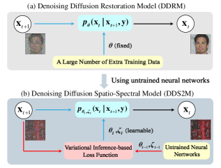
Figure 1: Comparison between DDRM and our self-supervised DDS2M. (a) DDRM utilizes a denoising network pre-trained on a large number of extra training data to reverse the diffusion process. (b) Our DDS2M works by inferring the untrained neural networks’ parameters $\{\bm{\theta},\bm{\zeta}\}$ during the reverse diffusion process, only using the degraded HSI $\mathbf{y}$ without any extra training data. The untrained neural networks and the variational inference-based loss function constitute the proposed Variational Spatio-Spectral Module (VS2M).

As a new trendy generative model, diffusion models [37, 13, 28, 38] have attracted significant attention in the community owing to their state-of-the-art performance in image synthesis [7]. In essence, diffusion model is a parameterized sampling chain trained using a variational bound objective, which is equivalent to that of score-based models [39, 40, 41]. After training, samples are generated by the sampling chain, starting from white noise and gradually denoising to a clean image.

Remarkably, diffusion models can go beyond image synthesis [11, 32, 20], and have been widely utilized in image restoration tasks, such as super-resolution [16, 46, 34, 6], inpainting [16, 46, 33, 21, 39, 41], denoising [16], and so on. Among these methods, DDRM [16], a diffusion-based image restoration framework, has achieved powerful robustness to noise, which is also noteworthy for hyperspectral images (HSIs). HSIs often suffer from noise corruption due to the limited light, photon effects, and atmospheric interference [19]. This motivates us to inherit the powerful noise robustness of DDRM [16] to HSI restoration by capitalizing on the power of diffusion model for HSI restoration.

However, harnessing the power of the diffusion model for HSI restoration is challenging. The bottleneck lies in the poor generalization ability to HSIs in various scenarios. Existing diffusion-based methods are excessively dependent on the adversity and quantity of the training data, and often focus on a specific domain, such as the face. As a result, these methods may perform very well in-distribution, but can be quite susceptible to distribution shifts, resulting in degraded performance. This is particularly inappropriate for data-poor applications such as HSI restoration, where very limited HSIs are available for training [27]. This is because HSIs are much more expensive to acquire in real-world scenarios, compared to natural RGB images. In addition, different sensors often admit large different specifications, such as the frequency band used, the spatial and spectral resolution. Therefore, a diffusion model trained on HSIs captured by one sensor may not be useful for HSIs captured by other sensors. In addition to the generalization ability issues mentioned above, how to leverage the intrinsic structure of HSIs is also critical for harnessing the power of the diffusion model for HSI restoration. Bearing the above concerns in mind, an effective diffusion model tailored for HSI restoration, which is able to generalize to HSIs in various practical scenarios and leverage the intrinsic structure of HSIs, is highly desired.

To address the generalization ability problem mentioned above, one remedy is to use the emerging untrained neural networks, such as those in [42, 36, 9]. These methods learn a generative neural network directly from a single degraded image, rather than from a large volume of external training data. The rationale is that an appropriate neural network architecture, without training data, could already encode much critical low-level image statistical prior information. Owing to their training data-independent nature, untrained networks can usually generalize well to the wild data. Meanwhile, due to our need to flexibly cope with various HSIs in real scenarios, untrained networks are rendered as a natural choice. In addition, their powerful expressiveness allows the deployment of such untrained networks in the diffusion models for HSI restoration.

In this work, we put force a self-supervised Denoising Diffusion Spatio-Spectral Model (DDS2M), which can cleverly alleviate the generalization ability problem, while exploiting the intrinsic structure information of the underlying HSIs. DDS2M is a denoising diffusion generative model that progressively and stochastically denoises samples into restored results conditioned on the degraded HSI and the degradation model after a finite time. Unlike existing diffusion models [37, 13, 38, 16, 46], which use a neural network pre-trained a large number of training data, DDS2M reverses the diffusion process by virtue of the proposed Variational Spatio-Spectral Module (VS2M), solely using the degraded HSI without any extra training data; see Figure 1 for visual comparison with DDRM [16].

Specifically, the proposed VS2M consists of two types of untrained networks (i.e., untrained spatial and spectral networks) and a customized variational inference-based loss function. The untrained spatial and spectral networks leverage the intrinsic structure of HSIs by modeling the abundance maps and endmembers derived from the linear mixture model [3], respectively. The variational inference-based loss function is customized to enable these untrained networks to learn the posterior distribution of the task at hand. The specific contributions of this work are summarized as follows:

$\bullet$ We propose a self-supervised Deep Diffusion Spatio-Spectral Model (DDS2M). Benefiting from its diffusion process and self-supervised nature, DDS2M enjoys stronger robustness to noise relative to existing HSI restoration methods and superior generalization ability to various HSIs relative to existing diffusion-based methods. To the best of our knowledge, DDS2M is the first self-supervised diffusion model that can restore HSI only using the degraded HSI without any additional training data.

$\bullet$ We design a variational spatio-spectral module (VS2M) to help reverse the diffusion process, which serves as the transitions of the sampling chain. VS2M is capable of approximating the posterior distribution of the task at hand by leveraging the intrinsic structure of the underlying HSI.

$\bullet$ Extensive experiments on HSI denoising, noisy HSI completion and super-resolution illustrate the superiority of DDS2M over the existing task-specific state-of-the-arts, especially in terms of the robustness to noise, and the generalization ability to HSIs in diverse scenarios.

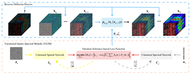
Figure 2: An overview of the proposed self-supervised DDS2M. In DDS2M, the diffusion process is reversed with the help of the proposed VS2M, solely using the degraded HSI without any extra training data. VS2M consists of the untrained spatial and spectral networks (aiming at leveraging the intrinsic structure of HSIs) and the variational inference-based loss function (aiming at enabling the untrained networks to learn the posterior distribution).

2 Related Works

2.1 HSI Restoration Methods

HSI restoration is a long-standing problem with a wide range of applications, with model-based approaches dominating the early years [55, 50, 53]. Recently, triggered by the expressive power of deep neural networks, a plethora of supervised [4, 10, 44] and self-supervised methods [36, 27] were developed.

The supervised methods mainly concentrate on exploring different neural network architectures to learn a mapping from a degraded HSI to the ground truth, such as convolution neural network [25, 54], recurrent neural network [8], and transformer [5, 19]. The main bottleneck of these supervised methods is that their performance is limited by the adversity and amount of training data, and is often susceptible to distribution outliers. In contrast, our DDS2M is not affected by such distribution outliers, since no extra training data is required in DDS2M.

Among the self-supervised methods, a representative family is the untrained neural network-based methods [36, 27]. As a promising tool for image restoration, untrained neural networks enjoy the expressive power of neural networks yet do not require additional training data [42]. Ulyanov et al. [42] first extended untrained neural network from RGB images to HSIs, putting forth a self-supervised HSI restoration framework. Then, Luo et al. [24] further proposed a spatio-spectral constrained untrained neural network. Inspired by these methods, Meng et al. [26] integrated untrained neural network into the plug-and-play regime [56]. In general, these methods learn a generator network directly from the degraded HSI in an iterative scheme. The critical drawback of these methods is that they easily accumulate errors inevitable in the iterative process, being quite fragile to degraded HSI with significant noise. Although our proposed DDS2M is also a multi-step generation process, it does not suffer from such accumulated errors. This is because diffusion-based methods have systematic mathematical formulation, and the errors in the intermediate step can be regarded as noise, which could be refined during the diffusion process [43]. Therefore, as compared with the above untrained network-based methods, our DDS2M is able to decently restore high-quality HSIs from the degraded HSI corrupted by noise.

2.2 Diffusion Models for Image Restoration

Recent emerged diffusion models have been widely utilized in image restoration. One branch of these works mainly focuses on tailoring a diffusion model suitable for a specific task, often leading to remarkable performance at the expense of flexibility across different tasks; see [34, 21, 47]. Another branch is concerned with tailoring a diffusion model that can be flexibly applied to different tasks; see [16, 46, 33]. To achieve this, these methods leave the training procedure intact, and only modify the inference procedure so that one can sample the restored image from a conditional distribution related to the task at hand. Among them, a representative method is DDRM [16], which achieves promising performance in multiple useful scenarios, including denoising, noisy super-resolution, and noisy completion, especially in terms of the robustness to noise.

However, the main shortcoming of these diffusion-based methods is their generalization ability to the wild data. These methods excessively depend on the adversity and amount of training data, and may perform very well in-distribution, but can be quite susceptible to distribution shifts, sometimes resulting in severely degraded performance. This becomes more problematic for data-poor applications such as HSI restoration. In this work, we aim to inherit the advantage of diffusion model (i.e., noise robustness) to HSI restoration, and boost its generalization ability to HSIs in practical scenarios.

3 Notations and Preliminaries

3.1 Notations

A scalar, a vector, a matrix, and a tensor are denoted as $x$, $\bf{x}$, $\bf{X}$, and $\mathcal{X}$, respectively. ${\bf x}^{(i)}$, ${\bf X}^{(i,j)}$, and ${\mathcal{X}}^{(i,j,k)}$ denote the $i$-th, $(i,j)$-th, and $(i,j,k)$-th element of $\mathbf{x}\in\mathbb{R}^{I}$, $\mathbf{X}\in\mathbb{R}^{I\times J}$, and $\mathcal{X}\in\mathbb{R}^{I\times J\times K}$, respectively. The Frobenius norms of $\bf{x}$ are denoted as $\|\bf{x}\|_{F}=\sqrt{\sum_{i}\bf{x}^{(i)}\bf{x}^{(i)}}$. Given $\mathbf{y}\in\mathbb{R}^{N}$ and a matrix $\mathbf{X}\in\mathbb{R}^{I\times J}$, the outer product is defined as $\mathbf{X}\circ\mathbf{y}$. In particular, $\mathbf{X}\circ\mathbf{y}\in\mathbb{R}^{I\times J\times N}$ and $(\mathbf{X}\circ\mathbf{y})^{(i,j,n)}=\mathbf{X}^{(i,j)}\mathbf{y}^{(n)}$. The ${\rm vec}(\mathbf{X})$ operator represents ${\rm vec}(\mathbf{X})=[\mathbf{X}^{(:,1)};\ldots;\mathbf{X}^{(:,J)}]\in\mathbb{R}^{IJ}$, and ${\rm vec}(\mathcal{X})$ is further defined as ${\rm vec}(\mathcal{X})=[{\rm vec}(\mathcal{X}^{(:,:,1)});\ldots;{\rm vec}(\mathcal{X}^{(:,:,K)})]\in\mathbb{R}^{IJK}$.

3.2 Degradation Model

The goal of HSI restoration is to recover a HSI from potentially noisy degraded HSI given through a known linear degradation model. In general, HSI restoration can be formulated as

$$\mathbf{y}=\mathbf{H}\mathbf{x}+\mathbf{z},$$ (1)

where $\mathbf{x}\in\mathbb{R}^{n}$ is the vector version of the original HSI $\mathcal{X}$ defined as $\mathbf{x}={\rm vec(\mathcal{X})}$, $\mathbf{y}\in\mathbb{R}^{m}$ is corresponding to the degraded HSI $\mathcal{Y}$ defined as $\mathbf{y}={\rm vec}(\mathcal{Y})$, $\mathbf{H}$ is the degradation matrix that depends on the restoration task at hand, and $\mathbf{z}\sim\mathcal{N}\left(0,\sigma_{\mathbf{y}}^{2}\bm{I}\right)$ represents an i.i.d. additive Gaussian noise with standard deviation $\sigma_{\mathbf{y}}$. It is worth noting that in this work, following previous diffusion-based methods [16, 13, 38, 21, 34, 47], $\mathbf{x}$ and $\mathbf{y}$ in Eqn. (1) are all scaled linearly to the range of $[-1,1]$, which ensures the neural network to operate on consistently scaled inputs during the reverse diffusion process. Therefore, when they are linearly scaled back to the range of $[0,1]$, the standard deviation of the Gaussian noise becomes $\sigma=0.5\sigma_{y}$.

4 Denoising Diffusion Spatio-Spectral Models

In this section, we introduce the proposed DDS2M. The key idea behind DDS2M is to reverse the diffusion process solely using the degraded HSI without extra training data, with the help of the proposed VS2M. We first give an introduction to the diffusion process for image restoration, then describe our design in VS2M, and finally elaborate on the VS2M-aided reverse diffusion process.

4.1 Diffusion Process for Image Restoration

Diffusion models for image restoration are generative models with Markov chain $\mathbf{x}_{T}\rightarrow\mathbf{x}_{T-1}\rightarrow\ldots\rightarrow\mathbf{x}_{1}\rightarrow\mathbf{x}_{0}$ conditioned on $\mathbf{y}$ [16], which has the following marginal distribution equivalent to that in [13, 38]:

$$q\left(\mathbf{x}_{t}|\mathbf{x}_{0}\right)=\mathcal{N}\left(\mathbf{x}_{t};\sqrt{\bar{\alpha}_{t}}\mathbf{x}_{0},\left(1-\bar{\alpha}_{t}\right)\mathbf{I}\right)$$ (2)

with

$$\alpha_{t}=1-\beta_{t},\quad\bar{\alpha}_{t}=\prod_{i=0}^{t}\alpha_{i},$$ (3)

where $\mathbf{x}_{0}$ and $\mathbf{y}$ are the vector version of high-quality HSI $\mathcal{X}$ and degraded HSI $\mathcal{Y}$, and $\beta_{t}$ is a hyperparameter. The forward process (i.e., diffusion process ) progressively injects Gaussian noise to the original data $\mathbf{x}_{0}$ and obtains $\mathbf{x}_{T}$ that looks indistinguishable from pure Gaussian noise, while the reverse diffusion process samples a slightly less noisy image $\mathbf{x}_{t}$ from $\mathbf{x}_{t+1}$ by leveraging the forward process posterior distribution $q\left(\mathbf{x}_{t}|\mathbf{x}_{t+1},\mathbf{x}_{0},\mathbf{y}\right)$. More details can be found in the supplementary materials.

In DDRM, denoising is performed using a network pre-trained on a large number of additional training data like other diffusion models [16, 13, 38, 21, 34, 47], which perform well in-distribution, and can be susceptible to distribution shift. This is especially inappropriate with data-starved HSI restoration. In this work we break this routine and propose to reverse the diffusion process utilizing the VS2M that can perform denoising solely using the degraded image without any extra training data.

4.2 Variational Spatio-Spectral Module (VS2M)

The VS2M utilized in DDS2M consists of untrained spatial and spectral networks, and a variational inference-based loss function. The untrained spatial and spectral networks are capable of leveraging the intrinsic structure of HSIs using designated network structures. The variational inference-based loss function is customized to enable these untrained networks to learn the posterior distribution. In this way, the untrained networks and the diffusion model can be incorporated to achieve promising performance.

Under VS2M, HSI $\mathcal{X}\in\mathbb{R}^{I\times J\times K}$ is represented as:

$$\mathcal{X}=\sum\nolimits_{r=1}^{R}\mathbf{S}_{r}\circ\mathbf{c}_{r},$$ (4)

where $\mathbf{c}_{r}\in\mathbb{R}^{K}$ and $\mathbf{S}_{r}\in\mathbb{R}^{I\times J}$ represent the $r$-th endmember and the $r$-th endmember’s abundance map, respectively, and $R$ is the number of endmembers contained in the HSI. More details about the decomposition in Eqn. (4) can be found in the supplementary materials. Here we introduce the untrained network architecture and the variational inference-based loss function individually.

Untrained Network Architecture. The physical interpretation of $\mathbf{S}_{r}$ and $\mathbf{c}_{r}$ makes it possible to utilize certain untrained networks to model these factors. Specifically, untrained U-Net-like “hourglass“ architecture in [42] and untrained full-connected networks (FCNs) are employed for abundance map modeling and endmember modeling, since abundance maps reveal similar qualities of the nature images [31] and the endmembers can be regarded as relatively simple 1D signals, as was done in [27]. Following this perspective, we model the HSI $\mathbf{x}\in\mathbb{R}^{IJK}$ as follows:

$${\mathbf{x}}={\rm vec}(\mathcal{X})={\rm vec}(\sum\nolimits_{r=1}^{R}{\cal S}_{\mathbf{\bm{\theta}}}(\mathbf{z}_{r})\circ{\cal C}_{\mathbf{\bm{\zeta}}}(\mathbf{w}_{r})),$$ (5)

where ${\cal S}_{\mathbf{\bm{\theta}}}(\cdot):\mathbb{R}^{N_{a}}\rightarrow\mathbb{R}^{I\times J}$ is the untrained U-Net-like network for abundance map generation, and $\bm{\theta}$ collects all the corresponding network weights; similarly, ${\cal C}_{{\bm{\zeta}}}(\cdot):\mathbb{R}^{N_{s}}\rightarrow\mathbb{R}^{K}$ and ${\bm{\zeta}}$ denote the untrained FCN for endmember generation and the corresponding network weights, respectively; the vectors $\mathbf{z}_{r}\in\mathbb{R}^{N_{a}}$ and $\mathbf{w}_{r}\in\mathbb{R}^{N_{s}}$ are low-dimensional random vectors that are responsible for generating the $r$-th abundance map and endmember respectively. $\mathbf{z}_{r}$ and $\mathbf{w}_{r}$ are randomly initialized but fixed during the optimization process. It is worth noting that, instead of directly using the vanilla U-Net structure for abundance map modeling, we propose to introduce the attention mechanism [48] into the U-Net, which aims to enhance the self-supervised expression ability of the VS2M. The concrete structure of the untrained spatial and spectral networks is illustrated in the supplementary materials.

Variational Inference-based Loss Function. We aim to estimate high-quality HSI $\mathbf{x}_{0}$ using the aforementioned untrained spatial and spectral networks, and update their parameters at every reverse process step. Denoting $\{{\bm{\theta}}_{t},{\bm{\zeta}}_{t}\}$ as the parameters at step $t$, we first define a learnable generative process $p_{\bm{\theta}_{t},\bm{\zeta}_{t}}\left(\mathbf{x}_{t}|\mathbf{x}_{t+1},\mathbf{y}\right)$ by replacing the $\mathbf{x}_{0}$ in $q\left(\mathbf{x}_{t}|\mathbf{x}_{t+1},\mathbf{x}_{0},\mathbf{x}\right)$ with ${\mathbf{x}}_{\bm{\theta}_{t},\bm{\zeta}_{t}}$, i.e.,

$$p_{\bm{\theta}_{t},\bm{\zeta}_{t}}\left(\mathbf{x}_{t}|\mathbf{x}_{t+1},\mathbf{y}\right)\triangleq q\left(\mathbf{x}_{t}|\mathbf{x}_{t+1},{\mathbf{x}}_{\bm{\theta}_{t},\bm{\zeta}_{t}},\mathbf{y}\right),$$ (6)

where ${\mathbf{x}}_{\bm{\theta}_{t},\bm{\zeta}_{t}}$ denotes the vector version of the estimated HSI at reverse process step $t$, i.e.,

$${\mathbf{x}}_{\bm{\theta}_{t},\bm{\zeta}_{t}}={\rm vec}(\sum\nolimits_{r=1}^{R}{\cal S}_{\bm{\theta}_{t}}(\mathbf{z}_{r})\circ{\cal C}_{\bm{\zeta}_{t}}(\mathbf{w}_{r}))$$ (7)

The goal of DDS2M is to find a set of parameters $\{{\bm{\theta}}_{t},{\bm{\zeta}}_{t}\}$ to make $p_{\bm{\theta}_{t},\bm{\zeta}_{t}}\left(\mathbf{x}_{t}|\mathbf{x}_{t+1},\mathbf{y}\right)$ as close to $q\left(\mathbf{x}_{t}|\mathbf{x}_{t+1},\mathbf{x}_{0},\mathbf{y}\right)$ as possible, by maximizing the variational lower bound of the log likelihood objective:

$$\mathbb{E}_{q\left(\mathbf{x}_{0}\right),q\left(\mathbf{y}\mid\mathbf{x}_{0}\right)}\left[\log p_{{\bm{\theta}},{\bm{\zeta}}}\left(\mathbf{x}_{0}|\mathbf{y}\right)\right]$$ (8)

$$\geq \mathbb{E}_{q\left(\mathbf{x}_{0:T}\right),q\left(\mathbf{y}|\mathbf{x}_{0}\right)}\left[\log p_{{\bm{\theta}},{\bm{\zeta}}}\left(\mathbf{x}_{0:T}|\mathbf{y}\right)-\log q\left(\mathbf{x}_{1:T}|\mathbf{x}_{0},\mathbf{y}\right)\right].$$

Notably, the objective in Eqn. (8) can be reduced into a denoising objective, i.e., estimating the underlying high-quality HSI $\mathbf{x}_{0}$ from the noisy $\mathbf{x}_{t}$ (please refer to the supplementary materials for derivation). By reparameterizing Eqn. (2) as

$$\mathbf{x}_{t}\left(\mathbf{x}_{0},\bm{\epsilon}\right)=\sqrt{\bar{\alpha}_{t}}\mathbf{x}_{0}+\sqrt{1-\bar{\alpha}_{t}}\epsilon\ \ \ \ \text{ for }\epsilon\sim\mathcal{N}(\mathbf{0},\mathbf{I}),$$ (9)

our variation inference-based loss function can be designed as follows:

$$\mathop{\arg\min}_{\{{\bm{\theta}},{\bm{\zeta}}\}}~{}\left\|\mathbf{x}_{t}-{\rm vec}(\sqrt{\bar{\alpha}_{t}}\sum\nolimits_{r=1}^{R}{{\cal S_{{\bm{\theta}}}}}({\mathbf{z}_{r}})\circ{\cal C_{{\bm{\zeta}}}}({\mathbf{w}_{r}}))\right\|_{F}^{2}.$$ (10)

Intuitively, given a noisy observation $\mathbf{x}_{t+1}$, after optimizing $\{\bm{\theta}_{t},\bm{\zeta}_{t}\}$ from $\mathbf{x}_{t+1}$ via Eqn. (10) using the Adam [18], $\mathbf{x}_{\bm{\theta}_{t},\bm{\zeta}_{t}}$ can be derived via Eqn. (7), and then $\mathbf{x}_{t}$ could be sampled from $p_{\bm{\theta}_{t},\bm{\zeta}_{t}}\left(\mathbf{x}_{t}|\mathbf{x}_{t+1},\mathbf{y}\right)$ defined in Eqn. (6). In this way, the diffusion process could be reversed in a self-supervised manner with no need for extra training data.

4.3 VS2M-Aided Reverse Diffusion Process

Given a degradation matric $\mathbf{H}\in\mathbb{R}^{m\times n}$, its singular value decomposition is posed as:

$$\mathbf{H}=\mathbf{U}\mathbf{\Sigma}\mathbf{V}^{\mathsf{T}},$$ (11)

where $\mathbf{U}\in\mathbb{R}^{m\times m}$, $\mathbf{V}\in\mathbb{R}^{n\times n}$ are orthogonal matrices, and $\mathbf{\Sigma}\in\mathbb{R}^{m\times n}$ is the rectangular diagonal matrix consisting of the singular values denoted as $s_{1}\geq s_{2}\geq\ldots\geq s_{n}$. The idea behind this is to tie the noise in the degraded signal $\mathbf{y}$ with the diffusion noise in $\mathbf{x}_{1:T}$, ensuring that the diffusion result $\mathbf{x}_{0}$ is faithful to the degraded signal $\mathbf{y}$ [17].

Before illustrating the reverse diffusion process in detail, we first rethink the difference between our DDS2M and other diffusion-based methods [13, 16] to guide the design of the reverse diffusion process. The main difference is how $\mathbf{x}_{0}$ is predicted from $\mathbf{x}_{t}$ at each reverse step. In [13, 16], a denoising network is trained on a large amount of additional training data to predict $\mathbf{x}_{0}$. By exploiting the external prior knowledge, this network could produce satisfactory $\mathbf{x}_{0}$ even if $\mathbf{x}_{t}$ looks like pure Gaussian noise. Because of this, such a denoising network could work during the whole reverse diffusion process. However, it is difficult for untrained networks to produce a satisfactory image by denoising an image that is almost pure Gaussian noise. Therefore, starting inference from pure Gaussian is unsuitable for our DDS2M.

Following the above argument, we propose to start inference from a single forward diffusion with better initialization, instead of starting from pure Gaussian noise [13, 16, 28, 38]. Specifically, we first perturb the degraded HSI $\mathbf{y}$ via the forward diffusion process up to $t_{0}<T$, where $t_{0}$ denotes the step that the reverse diffusion process starts from. Denoting $\bar{\mathbf{x}}^{(i)}$ as the $i$-th index of vector $\bar{\mathbf{x}}_{t}=\mathbf{V}^{\mathsf{T}}\mathbf{x}_{t}$, $\bar{\mathbf{y}}^{(i)}$ as the $i$-th index of $\bar{\mathbf{y}}=\mathbf{\Sigma}^{\dagger}\mathbf{U}^{\mathsf{T}}\mathbf{y}$, and $\bar{\mathbf{x}}_{{\bm{\theta}}_{t},{\bm{\zeta}}_{t}}^{(i)}$ as the $i$-th index of $\bar{\mathbf{x}}_{{\bm{\theta}}_{t},{\bm{\zeta}}_{t}}=\mathbf{V}^{\mathsf{T}}\mathbf{x}_{{\bm{\theta}}_{t},{\bm{\zeta}}_{t}}$, for all $t<t_{0}$, the variational distribution is defined as:

$$p_{\bm{\theta}_{t_{0}},\bm{\zeta}_{t_{0}}}\left(\bar{\mathbf{x}}_{t_{0}}^{(i)}|\mathbf{y}\right)=\begin{cases}\mathcal{N}(\bar{\mathbf{y}}^{(i)},\sigma_{t_{0}}^{2}-\frac{\sigma_{y}^{2}}{s_{i}^{2}})&\text{ if }s_{i}>0\\ \mathcal{N}(0,\sigma_{t_{0}}^{2})&\text{ if }s_{i}=0\end{cases}$$ (12)

$$p_{\bm{\theta}_{t},\bm{\zeta}_{t}}(\bar{\mathbf{x}}_{t}^{(i)}|\mathbf{x}_{t+1},\mathbf{y})=$$ (13)

$$\begin{cases}\mathcal{N}(\bar{\mathbf{x}}_{\bm{\theta}_{t},\bm{\zeta}_{t}}^{(i)}+\sqrt{1-\eta^{2}}\sigma_{t}\frac{\bar{\mathbf{x}}_{t+1}^{(i)}-\bar{\mathbf{x}}_{\bm{\theta}_{t},\bm{\zeta}_{t}}^{(i)}}{\sigma_{t+1}},\eta^{2}\sigma_{t}^{2})&\text{ if }s_{i}=0\\ \mathcal{N}(\bar{\mathbf{x}}_{\bm{\theta}_{t},\bm{\zeta}_{t}}^{(i)}+\sqrt{1-\eta^{2}}\sigma_{t}\frac{\bar{\mathbf{y}}^{(i)}-\bar{\mathbf{x}}_{\bm{\theta}_{t},\bm{\zeta}_{t}}^{(i)}}{\sigma_{\mathbf{y}}/s_{i}},\eta^{2}\sigma_{t}^{2})&\text{ if }\sigma_{t}<\frac{\sigma_{\mathbf{y}}}{s_{i}}\\ \mathcal{N}(\left(1-\eta_{b}\right)\bar{\mathbf{x}}_{\bm{\theta}_{t},\bm{\zeta}_{t}}^{(i)}+\eta_{b}\bar{\mathbf{y}}^{(i)},\sigma_{t}^{2}-\frac{\sigma_{\mathbf{y}}^{2}}{s_{i}^{2}}\eta_{b}^{2})&\text{ if }\sigma_{t}\geq\frac{\sigma_{\mathbf{y}}}{s_{i}}\end{cases}$$

where $\sigma_{t}$ depending on the hyperparameter $\beta_{1:T}$ denotes the variance of diffusion noise in $\mathbf{x}_{t}$, and $\eta$, $\eta_{b}$ are the hyperparameters, which control the level of noise injected at each timestep. Once $\bar{\mathbf{x}}_{{\bm{\theta}}_{t},{\bm{\zeta}}_{t}}$ is sampled from Eqn. (13), it is easy to obtain $\mathbf{x}_{{\bm{\theta}}_{t},{\bm{\zeta}}_{t}}$ exactly by left multiplying $\mathbf{V}$. And the values of the parameters $\{\bm{\theta}_{t_{0}},\bm{\zeta}_{t_{0}}\}$ are randomly initialized.

It is worth noting that the parameter updating (i.e, $\{\bm{\theta},\bm{\zeta}\}$) and the reverse diffusion process are iteratively performed. The parameter values of each reverse diffusion step are inherited from the previous step, thus the parameters can be updated continuously during the reverse diffusion process. This reverse diffusion process is summarized in Algorithm 1.

Algorithm 1 Reverse Diffusion Process of DDS2M.

1:The degraded HSI $\mathbf{y}$, the hyperparameter $R$, $t_{0}$, $T$, $\beta_{1:t_{0}}$, $\sigma_{1:t_{0}}$, $\sigma_{y}$, $\eta$ and $\eta_{b}$.

2:Randomly initialize $\bm{\theta}_{t_{0}}$, $\bm{\zeta}_{t_{0}}$,$\mathbf{z}_{r}$, and $\mathbf{w}_{r}$ ;

3:Obtain $\mathbf{x}_{t_{0}}$ via reparameterizing Eqn. (12);

4:for $t=t_{0}-1$ to 1 do

5:     Update $\{\bm{\theta}_{t},\bm{\zeta}_{t}\}$ via Eqn. (10);

6:     Obtain ${\mathbf{x}}_{\bm{\theta}_{t},\bm{\zeta}_{t}}$ via Eqn. (7);

7:     Obtain $\mathbf{x}_{t-1}$ via reparameterizing Eqn. (13);

8:end for

9:The restored HSI $\mathbf{x}_{0}$.

5 Experiments

5.1 Comparisons with State-of-the-Arts

In this paper, our interest lies in inheriting the DDRM’s powerful robustness to noise (which is unavoidable in the hyperspectral imaging process) to HSI restoration. Herein we mainly consider noisy HSI completion, HSI denoising, and noisy HSI super-resolution, and compare the proposed DDS2M with the existing task-specific state-of-the-arts. Two frequently used evaluation metrics, namely, peak signal-to-noise ratio (PSNR) and structure similarity (SSIM), are adopted to evaluate the results. In general, better performance is reflected by higher PSNR and SSIM values. In DDS2M, $T$ is set as {3000, 1000, 1000} for noisy HSI completion, HSI denoising, and noisy HSI super-resolution, respectively, and the step $t_{0}$ to start reverse the diffusion process is set as $T/2$. We use $\eta=0.95,\eta_{b}=1$, and linearly increase $\beta_{1:T}$ in which $\beta_{1}=10^{-4}$ and $\beta_{T}$ = $\{2\times 10^{-3},5\times 10^{-3}\}$. The variance $\sigma_{t}$ is set as a constant $\sigma_{t}=\frac{1-\bar{\alpha}_{t-1}}{1-\bar{\alpha}_{t}}\beta_{t}$ for all experiments. The number of endmembers $R$ is selected from $\{5,10\}$. As for diffusion-based restoration methods DDNM [46] and DDRM [16], the diffusion model in them is trained on a large-scale remote sensing imagery dataset AID [49] containing ten thousands of scene images, and HSI restoration is performed in a channel-by-channel manner. All of the compared methods’ parameters are set as suggested by the authors, with parameter fine-tuning efforts to uplift their performance. For implementation details, parameters sensitivity analysis, and inference time analysis, please refer to the supplementary materials.

5.1.1 Datasets and Compared Methods

Noisy HSI Completion. The noisy HSI completion aims at recovering the underlying HSI from the noisy incompleted observation. We adopt a wide range of HSIs to conduct the experiments, including 32 natural HSIs (i.e., CAVE dataset [51]), and 3 remote sensing HSIs (i.e., WDC Mall, Pavia Centre, and Pavia University datasets). The sampling rates are set as {0.1, 0.2, 0.3}, and the standard deviation $\sigma$ of Gaussian noise in the range of [0,1] is set as 0.1. The compared methods consist of seven model-based methods (i.e., TMac-TT [2], TNN [57], TRLRF [53], FTNN [15], TCTF [58], SN2TNN [23], and HLRTF [22]), two unsupervised deep learning-based methods (i.e., DIP2D [36] and DIP3D [36]), and two diffusion-based methods (i.e., DDRM [16] and DDNM [46]).

HSI Denoising. The HSI denoising aims at recovering the clean HSI from its noisy observation. The data adopted in this experiment is the same as that in HSI completion, including 32 natural HSIs and 3 remote sensing HSIs. Herein we mainly consider Gaussian noise, and the standard deviation of Gaussian noise $\sigma$ in the range of $[0,1]$ is set as $\{0.1,0.2,0.3\}$. The compared methods consist of six model-based methods (i.e., LRMR [55], LRTDTV [45], LRTFL0 [50], E3DTV [29], HLRTF [22], and NGMeet [12]), two unsupervised deep learning-based methods (i.e., DIP2D [36] and DIP3D [36]), and a supervised deep learning-based method (i.e., SST [19]). Since the purpose of the comparison with supervised methods in this work is to highlight the generalization ability of our methods, we directly use the models of SST trained on ICVL [1] with Gaussian noise provided by the authors.

Noisy HSI Super-Resolution. The noisy HSI super-resolution aims at recovering high-resolution HSI from its noisy low-resolution counterpart. We adopt CAVE dataset [51] to conduct the experiments. The scale factor is set as $\times$2, $\times$4, and $\times$8, and the standard deviation of Gaussian noise $\sigma$ in the range of $[0,1]$ is set as 0.1. The compared methods include three supervised deep learning-based methods (i.e., SFCSR [30], RFSR [44], and SSPSR [14]), a model-based method (i.e., LRTV [35]), two unsupervised deep learning-based methods (i.e., DIP2D [36] and DIP3D [36]), and a diffusion-based method (i.e., DDRM [16]). In order to comprehensively compare with supervised methods in terms of generalization ability to other datasets and other noise standard deviations, we train each supervised model under five different settings, i.e., CAVE without noise denoted as xxx(0), CAVE with 0.1 Gaussian noise denoted as xxx(0.1), CAVE with 0.05 Gaussian noise denoted as xxx(0.05), CAVE with 0.03 Gaussian noise denoted as xxx(0.03), and Chikusei dataset [52] with 0.1 Gaussian noise denoted as xxx(0.1)*. Here xxx denotes the method name, i.e., SFCSR, RFSR, and SSPSR.

5.1.2 Experimental Results

Table 1: The average quantitative results for noisy HSI completion. The best and second-best values are highlighted.

Sampling Rate		0.1		0.2		0.3
Dataset	Method	PSNR	SSIM	PSNR	SSIM	PSNR	SSIM
	TNN	23.841	0.334	24.241	0.333	24.361	0.333
	TMac-TT	21.516	0.473	21.104	0.439	21.501	0.407
	TRLRF	26.745	0.548	27.968	0.626	28.427	0.655
	DIP2D	28.621	0.676	29.412	0.693	29.971	0.704
Natural HSI	DIP3D	24.938	0.592	25.273	0.603	25.342	0.606
CAVE Dataset	FTNN	25.071	0.459	26.293	0.495	26.923	0.515
consists of 32 HSIs	FCTN	26.778	0.578	27.547	0.631	27.812	0.649
each with a size of	SN2TNN	25.883	0.532	27.236	0.585	28.101	0.617
$256\times 256\times 31$	HLRTF	29.514	0.700	30.076	0.725	30.728	0.748
	DDNM	16.718	0.260	27.847	0.607	32.222	0.818
	DDRM	24.474	0.655	28.151	0.785	29.868	0.827
	DDS2M	32.507	0.871	34.156	0.896	35.098	0.909
	TNN	23.031	0.478	23.030	0.488	22.721	0.479
	TMac-TT	21.859	0.411	22.026	0.417	21.640	0.390
	TRLRF	25.402	0.644	25.772	0.666	25.901	0.675
Remote Sensing HSI	DIP2D	28.392	0.786	30.600	0.857	31.608	0.882
WDC Mall	DIP3D	22.204	0.399	22.169	0.402	22.512	0.405
$256\times 256\times 191$	FTNN	23.956	0.523	25.575	0.619	26.457	0.666
Pavia Centre	FCTN	24.352	0.586	24.523	0.599	24.591	0.604
$256\times 256\times 87$	SN2TNN	28.567	0.797	30.513	0.848	31.507	0.873
Pavia University	HLRTF	29.272	0.825	31.001	0.869	31.938	0.891
$192\times 192\times 80$	DDNM	21.002	0.343	23.445	0.534	25.758	0.657
	DDRM	21.423	0.371	23.467	0.495	24.771	0.587
	DDS2M	30.277	0.857	32.179	0.900	33.208	0.918

Table 2: The average quantitative results for HSI denoising. The best and second-best values are highlighted.

standard deviation		0.1		0.2		0.3
Dataset	Method	PSNR	SSIM	PSNR	SSIM	PSNR	SSIM
	LRMR	30.948	0.754	27.718	0.600	25.698	0.496
	LRTDTV	37.354	0.937	33.598	0.863	30.098	0.725
	LRTFL0	34.205	0.872	29.551	0.722	26.155	0.641
	DIP2D	30.498	0.742	24.663	0.605	20.808	0.513
Natural HSI	DIP3D	27.965	0.677	23.759	0.559	20.407	0.485
CAVE Dataset	NGMeet	31.698	0.772	24.964	0.621	20.657	0.517
consists of 32 HSIs	E3DTV	33.652	0.922	30.752	0.876	29.044	0.836
each with a size of	HLRTF	37.095	0.935	33.623	0.881	31.661	0.836
$256\times 256\times 31$	SST	29.803	0.757	24.519	0.627	20.866	0.542
	DDNM	29.223	0.615	24.148	0.353	21.104	0.226
	DDRM	33.391	0.895	29.987	0.831	27.935	0.782
	DDS2M	38.021	0.944	34.879	0.902	32.951	0.871
	LRMR	28.223	0.838	26.950	0.776	25.677	0.708
	LRTDTV	32.793	0.906	30.017	0.835	28.252	0.771
	LRTFL0	35.392	0.953	31.907	0.888	29.485	0.821
Remote Sensing HSI	DIP2D	30.991	0.872	27.195	0.801	23.067	0.731
WDC Mall	DIP3D	25.973	0.625	24.087	0.559	21.730	0.505
$256\times 256\times 191$	NGMeet	36.149	0.956	28.308	0.857	23.313	0.718
Pavia Centre	E3DTV	33.837	0.929	30.167	0.850	28.098	0.785
$256\times 256\times 87$	HLRTF	34.987	0.932	31.359	0.870	29.431	0.780
Pavia University	SST	34.625	0.932	27.487	0.820	22.821	0.709
$192\times 192\times 80$	DDNM	26.855	0.687	22.433	0.439	19.661	0.287
	DDRM	29.043	0.806	26.037	0.661	24.341	0.551
	DDS2M	36.548	0.959	32.925	0.911	30.863	0.867

Table 3: The average quantitative results for noisy HSI super-resolution on CAVE dataset. The best and second-best values are highlighted.

Scale		$\times$2		$\times$4		$\times$8
Method	Trained	PSNR	SSIM	PSNR	SSIM	PSNR	SSIM
SFCSR(0)	✔	16.615	0.198	16.829	0.155	17.070	0.148
SFCSR(0.03)	✔	24.193	0.508	23.859	0.508	22.277	0.472
SFCSR(0.05)	✔	27.620	0.688	25.142	0.625	22.953	0.587
SFCSR(0.1)	✔	30.350	0.856	26.302	0.744	23.342	0.609
SFCSR(0.1)*	✔	28.015	0.821	24.153	0.661	22.011	0.569
RFSR(0)	✔	18.570	0.252	18.412	0.206	18.045	0.181
RFSR(0.03)	✔	26.904	0.660	24.639	0.619	23.023	0.576
RFSR(0.05)	✔	29.591	0.814	26.187	0.732	23.248	0.602
RFSR(0.1)	✔	30.570	0.868	26.479	0.748	23.386	0.614
RFSR(0.1)*	✔	27.994	0.804	24.082	0.658	21.033	0.541
SSPSR(0)	✔	18.916	0.261	19.465	0.223	18.636	0.204
SSPSR(0.03)	✔	28.371	0.729	25.351	0.654	22.899	0.573
SSPSR(0.05)	✔	29.799	0.830	26.101	0.715	23.195	0.623
SSPSR(0.1)	✔	30.294	0.868	26.824	0.748	23.338	0.627
SSPSR(0.1)*	✔	27.636	0.828	24.748	0.705	21.465	0.585
Bicubic	✘	21.554	0.245	20.893	0.228	20.021	0.238
LRTV	✘	20.867	0.321	19.690	0.291	18.490	0.280
DIP2D	✘	28.344	0.745	25.238	0.602	22.613	0.482
DIP3D	✘	27.458	0.756	24.776	0.635	21.935	0.506
DDRM	✘	27.330	0.741	23.244	0.552	18.883	0.418
DDS2M	✘	30.997	0.859	26.835	0.748	23.621	0.626

The quantitative results of noisy HSI completion, HSI denoising, and noisy HSI super-resolution are reported in Tables 1, 2, and 3. We can observe that the proposed DDS2M outperforms existing model-based, unsupervised deep learning-based, and diffusion-based methods in all three tasks, while yielding competitive results with respect to the state-of-the-art supervised deep learning-based methods. Specifically, as compared with the diffusion-based method DDRM, our method offers average PSNR improvement of 5.878 dB, 5.909 dB, and 3.998 dB in completion, denoising, and super-resolution, respectively. This observation validates that DDS2M can more flexibly adapt to diverse HSIs in real scenarios. Additionally, in HSI super-resolution experiments, the supervised methods (i.e., SFCSR, RFSR, and SSPSR) all perform best when trained with CAVE dataset with 0.1 Gaussian noise among the five different training settings, and their performance degrades significantly when trained with other noise levels or datasets. It is worth noting that, our DDS2M achieves comparable performance with the best version of these supervised methods, and outperforms the models trained with other settings. This demonstrates the superiority of our DDS2M against these supervised methods.

Observed	DIP2D	DIP3D	FTNN	FCTN	S2NTNN	HLRTF	DDRM	DDS2M	Original
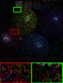
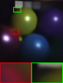
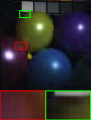
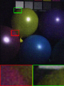
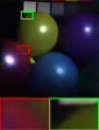
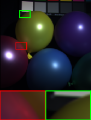
PSNR 14.582	PSNR 33.604	PSNR 28.707	PSNR 27.877	PSNR 30.393	PSNR 28.829	PSNR 32.778	PSNR 32.285	PSNR 37.886	PSNR Inf

Figure 3: The results of noisy HSI completion by different methods on HSI Balloons (sampling rate=0.3, $\sigma$=0.1).

Observed	NGMeet	DIP2D	DIP3D	LRTFL0	E3DTV	HLRTF	DDRM	DDS2M	Original
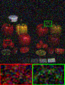
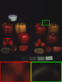
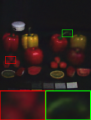
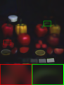
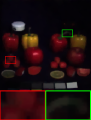
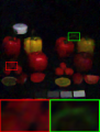
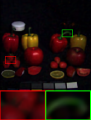
PSNR 16.423	PSNR 23.626	PSNR 23.855	PSNR 23.087	PSNR 30.383	PSNR 32.585	PSNR 33.658	PSNR 30.609	PSNR 34.721	PSNR Inf

Figure 4: The results of HSI denoising by different methods on HSI Fruits ($\sigma$=0.2).

Bicubic	LRTV	DIP2D	DIP3D	SSPSR	SFCSR	RFSR	DDRM	DDS2M	Original
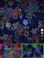
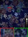
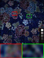
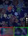
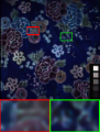
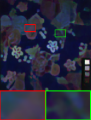
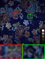
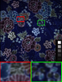
PSNR 17.875	PSNR 21.446	PSNR 24.175	PSNR 22.991	PSNR 24.355	PSNR 24.328	PSNR 24.575	PSNR 22.461	PSNR 25.485	PSNR Inf

Figure 5: The results of noisy HSI super-resolution by different methods on HSI Cloth (scale factor=$\times$2, $\sigma$=0.1).

Some visual results for different tasks are shown in Figures 3, 4, and 5. As observed, the proposed DDS2M is capable of preserving the most detailed information and demonstrating the best visual performance among the compared methods, which is consistent with its satisfactory performance in PSNR and SSIM. In addition, there is the least residual noise remaining in the results produced by DDS2M, which demonstrates the superiority of DDS2M in terms of noise robustness.

We conjecture that such promising results can be attributed to the organic cooperation of untrained spatial and spectral networks and diffusion model, which is beneficial to the generalization ability to various HSIs and the robustness to noise.

5.2 Ablation Study

We test the impact of untrained spatial and spectral networks, and diffusion process in DDS2M. The compared methods are listed as follows:
$\bullet$ DDS2M without untrained spatial and spectral networks (dubbed DDS2M w/o untra.): To evaluate the impact of the untrained spatial and spectral networks, we remove the untrained spatial and spectral networks, and use an untrained U-Net to directly generate the whole HSI.
$\bullet$ DDS2M without diffusion process (dubbed DDS2M w/o diffu.): To clarify the influence of the diffusion process, we remove the diffusion process and make the untrained spatial and spectral networks directly fit the degraded HSI in an iterative scheme.

We consider HSI denoising ($\sigma$=0.3), noisy HSI completion (sampling rate=0.1, $\sigma$=0.1), and noisy HSI super-resolutin (scale factor=2, $\sigma$=0.1). HSI Fruits from the CAVE dataset is selected as an example. The results are shown in Table 4. We can observe that the untrained spatial and spectral networks, and the diffusion process could indeed significantly boost the restoration performance. More implementation details can be found in the supplementary materials.

Table 4: The quantitative ablation results on HSI completion, denoising, and super-resolution. The best values are highlighted.

Task	Denoising		Completion		Super-Resolution
Methods	PSNR	SSIM	PSNR	SSIM	PSNR	SSIM
DDS2M w/o diffu.	31.983	0.738	31.562	0.739	31.172	0.730
DDS2M w/o untra.	29.682	0.643	28.565	0.593	32.588	0.808
DDS2M	33.045	0.841	33.217	0.845	34.066	0.876

6 Conclusion

This work reveals a new insight on how to synergistically integrate existing diffusion models with untrained neural networks, and puts forth a self-supervised diffusion model for HSI restoration, namely Denoising Diffusion Spatio-Spectral Model (DDS2M). By virtue of our proposed Variational Spatio-Spectral Module (VS2M), the diffusion process can be reversed solely using the degraded HSI without any extra training data. Benefiting from its self-supervised nature and diffusion process, DDS2M admits stronger generalization ability to various HSIs relative to existing diffusion-based methods and superior robustness to noise relative to existing HSI restoration methods.

References

- [1] Boaz Arad and Ohad Ben-Shahar. Sparse recovery of hyperspectral signal from natural rgb images. In ECCV, pages 19–34. Springer, 2016.
- [2] Johann A Bengua, Ho N Phien, Hoang Duong Tuan, and Minh N Do. Efficient tensor completion for color image and video recovery: Low-rank tensor train. IEEE Trans. Image Process., 26(5):2466–2479, 2017.
- [3] J. M. Bioucas-Dias, A. Plaza, N. Dobigeon, M. Parente, Q. Du, P. Gader, and J. Chanussot. Hyperspectral unmixing overview: Geometrical, statistical, and sparse regression-based approaches. IEEE J. Sel. Topics Appl. Earth Observ. Remote Sens., 5(2):354–379, 2012.
- [4] Theo Bodrito, Alexandre Zouaoui, Jocelyn Chanussot, and Julien Mairal. A trainable spectral-spatial sparse coding model for hyperspectral image restoration. NeurIPS, 2021.
- [5] Hongyu Chen, Guangyi Yang, and Hongyan Zhang. Hider: A hyperspectral image denoising transformer with spatial–spectral constraints for hybrid noise removal. IEEE Trans. Neural Netw. Learn. Syst., 2022.
- [6] Jooyoung Choi, Sungwon Kim, Yonghyun Jeong, Youngjune Gwon, and Sungroh Yoon. Ilvr: Conditioning method for denoising diffusion probabilistic models. In ICCV, pages 14347–14356. IEEE, 2021.
- [7] Prafulla Dhariwal and Alexander Nichol. Diffusion models beat GANs on image synthesis. In NeurIPS, volume 34, pages 8780–8794, 2021.
- [8] Ying Fu, Zhiyuan Liang, and Shaodi You. Bidirectional 3d quasi-recurrent neural network for hyperspectral image super-resolution. IEEE J. Sel. Topics Appl. Earth Observ. Remote Sens., 14:2674–2688, 2021.
- [9] Yosef Gandelsman, Assaf Shocher, and Michal Irani. ”Double-Dip”: Unsupervised image decomposition via coupled deep-image-priors. In CVPR, pages 11026–11035. IEEE, 2019.
- [10] Zhaori Gong, Nannan Wang, De Cheng, Xinrui Jiang, Jingwei Xin, Xi Yang, and Xinbo Gao. Learning deep resonant prior for hyperspectral image super-resolution. IEEE Trans. Geosci. Remote Sens., 60:1–14, 2022.
- [11] Shuyang Gu, Dong Chen, Jianmin Bao, Fang Wen, Bo Zhang, Dongdong Chen, Lu Yuan, and Baining Guo. Vector quantized diffusion model for text-to-image synthesis. In CVPR, pages 10696–10706, June 2022.
- [12] Wei He, Quanming Yao, Chao Li, Naoto Yokoya, and Qibin Zhao. Non-local meets global: An integrated paradigm for hyperspectral denoising. In CVPR, pages 6868–6877, 2019.
- [13] Jonathan Ho, Ajay Jain, and Pieter Abbeel. Denoising diffusion probabilistic models. NeurIPS, 33:6840–6851, 2020.
- [14] J. Jiang, H. Sun, X. Liu, and J. Ma. Learning spatial-spectral prior for super-resolution of hyperspectral imagery. IEEE Trans. Comput. Imag., 6:1082–1096, 2020.
- [15] Tai-Xiang Jiang, Michael K Ng, Xi-Le Zhao, and Ting-Zhu Huang. Framelet representation of tensor nuclear norm for third-order tensor completion. IEEE Trans. Image Process., 29:7233–7244, 2020.
- [16] Bahjat Kawar, Michael Elad, Stefano Ermon, and Jiaming Song. Denoising diffusion restoration models. In ICLR Workshops, 2022.
- [17] Bahjat Kawar, Gregory Vaksman, and Michael Elad. Snips: Solving noisy inverse problems stochastically. NeurIPS, 34:21757–21769, 2021.
- [18] Diederick P Kingma and Jimmy Ba. Adam: A method for stochastic optimization. In ICLR, 2015.
- [19] Miaoyu Li, Ying Fu, and Yulun Zhang. Spatial-spectral transformer for hyperspectral image denoising. In AAAI, 2023.
- [20] Xihui Liu, Dong Huk Park, Samaneh Azadi, Gong Zhang, Arman Chopikyan, Yuxiao Hu, Humphrey Shi, Anna Rohrbach, and Trevor Darrell. More control for free! image synthesis with semantic diffusion guidance. In Proceedings of the IEEE/CVF Winter Conference on Applications of Computer Vision, pages 289–299, 2023.
- [21] Andreas Lugmayr, Martin Danelljan, Andres Romero, Fisher Yu, Radu Timofte, and Luc Van Gool. Repaint: Inpainting using denoising diffusion probabilistic models. In CVPR, pages 11461–11471. IEEE, 2022.
- [22] Yisi Luo, Xi-Le Zhao, Deyu Meng, and Tai-Xiang Jiang. Hlrtf: Hierarchical low-rank tensor factorization for inverse problems in multi-dimensional imaging. In CVPR, pages 19303–19312. IEEE, 2022.
- [23] Yi-Si Luo, Xi-Le Zhao, Tai-Xiang Jiang, Yi Chang, Michael K Ng, and Chao Li. Self-supervised nonlinear transform-based tensor nuclear norm for multi-dimensional image recovery. IEEE Trans. Image Process., 31:3793–3808, 2022.
- [24] Yi-Si Luo, Xi-Le Zhao, Tai-Xiang Jiang, Yu-Bang Zheng, and Yi Chang. Hyperspectral mixed noise removal via spatial-spectral constrained unsupervised deep image prior. IEEE J. Sel. Topics Appl. Earth Observ. Remote Sens., 14:9435–9449, 2021.
- [25] Alessandro Maffei, Juan M Haut, Mercedes Eugenia Paoletti, Javier Plaza, Lorenzo Bruzzone, and Antonio Plaza. A single model CNN for hyperspectral image denoising. IEEE Trans. Geosci. Remote Sens., 58(4):2516–2529, 2019.
- [26] Ziyi Meng, Zhenming Yu, Kun Xu, and Xin Yuan. Self-supervised neural networks for spectral snapshot compressive imaging. In ICCV, pages 2622–2631, 2021.
- [27] Yu-Chun Miao, Xi-Le Zhao, Xiao Fu, Jian-Li Wang, and Yu-Bang Zheng. Hyperspectral denoising using unsupervised disentangled spatiospectral deep priors. IEEE Trans. Geosci. Remote Sens., 60:1–16, 2021.
- [28] Alexander Quinn Nichol and Prafulla Dhariwal. Improved denoising diffusion probabilistic models. In ICML, pages 8162–8171, 2021.
- [29] Jiangjun Peng, Qi Xie, Qian Zhao, Yao Wang, Leung Yee, and Deyu Meng. Enhanced 3dtv regularization and its applications on hsi denoising and compressed sensing. IEEE Trans. Image Process., 29:7889–7903, 2020.
- [30] Q. Li Q. Wang and X. Li. Hyperspectral image super-resolution using spectrum and feature context. IEEE Trans. Ind. Electron., 2020.
- [31] Yuntao Qian, Fengchao Xiong, Shan Zeng, Jun Zhou, and Yuan Yan Tang. Matrix-vector nonnegative tensor factorization for blind unmixing of hyperspectral imagery. IEEE Trans. Geosci. Remote Sens., 55(3):1776–1792, 2016.
- [32] Robin Rombach, Andreas Blattmann, Dominik Lorenz, Patrick Esser, and Björn Ommer. High-resolution image synthesis with latent diffusion models. In Proceedings of the IEEE/CVF Conference on Computer Vision and Pattern Recognition (CVPR), pages 10684–10695, June 2022.
- [33] Chitwan Saharia, William Chan, Huiwen Chang, Chris Lee, Jonathan Ho, Tim Salimans, David Fleet, and Mohammad Norouzi. Palette: Image-to-image diffusion models. In ACM SIGGRAPH, pages 1–10, 2022.
- [34] Chitwan Saharia, Jonathan Ho, William Chan, Tim Salimans, David J Fleet, and Mohammad Norouzi. Image super-resolution via iterative refinement. arXiv preprint arXiv:2104.07636, 2021.
- [35] Feng Shi, Jian Cheng, Li Wang, Pew-Thian Yap, and Dinggang Shen. Lrtv: Mr image super-resolution with low-rank and total variation regularizations. IEEE Trans. Med. Imag., 34(12):2459–2466, 2015.
- [36] Oleksii Sidorov and Jon Yngve Hardeberg. Deep hyperspectral prior: Single-image denoising, inpainting, super-resolution. In ICCV Workshops, pages 0–0. IEEE, 2019.
- [37] Jascha Sohl-Dickstein, Eric Weiss, Niru Maheswaranathan, and Surya ICMLGanguli. Deep unsupervised learning using nonequilibrium thermodynamics. In ICML, pages 2256–2265. PMLR, 2015.
- [38] Jiaming Song, Chenlin Meng, and Stefano Ermon. Denoising diffusion implicit models. In ICLR, 2021.
- [39] Yang Song and Stefano Ermon. Generative modeling by estimating gradients of the data distribution. NeurIPS, 32, 2019.
- [40] Yang Song and Stefano Ermon. Improved techniques for training score-based generative models. NeurIPS, 33:12438–12448, 2020.
- [41] Yang Song, Jascha Sohl-Dickstein, Diederik P Kingma, Abhishek Kumar, Stefano Ermon, and Ben Poole. Score-based generative modeling through stochastic differential equations. In ICLR, 2021.
- [42] Dmitry Ulyanov, Andrea Vedaldi, and Victor Lempitsky. Deep image prior. In CVPR, pages 9446–9454. IEEE, 2018.
- [43] Weilun Wang, Jianmin Bao, Wengang Zhou, Dongdong Chen, Dong Chen, Lu Yuan, and Houqiang Li. Sindiffusion: Learning a diffusion model from a single natural image. arXiv preprint arXiv:2211.12445, 2022.
- [44] Xinya Wang, Jiayi Ma, and Junjun Jiang. Hyperspectral image super-resolution via recurrent feedback embedding and spatial–spectral consistency regularization. IEEE Trans. Geosci. Remote Sens., 60:1–13, 2021.
- [45] Yao Wang, Jiangjun Peng, Qian Zhao, Yee Leung, Xi-Le Zhao, and Deyu Meng. Hyperspectral image restoration via total variation regularized low-rank tensor decomposition. IEEE J. Sel. Topics Appl. Earth Observ. Remote Sens., 11(4):1227–1243, 2017.
- [46] Yinhuai Wang, Jiwen Yu, and Jian Zhang. Zero-shot image restoration using denoising diffusion Null-space model. arXiv preprint arXiv:2212.00490, 2022.
- [47] Jay Whang, Mauricio Delbracio, Hossein Talebi, Chitwan Saharia, Alexandros G Dimakis, and Peyman Milanfar. Deblurring via stochastic refinement. In CVPR, pages 16293–16303. IEEE, 2022.
- [48] Sanghyun Woo, Jongchan Park, Joon-Young Lee, and In So Kweon. Cbam: Convolutional block attention module. In ECCV, pages 3–19, 2018.
- [49] Gui-Song Xia, Jingwen Hu, Fan Hu, Baoguang Shi, Xiang Bai, Yanfei Zhong, Liangpei Zhang, and Xiaoqiang Lu. Aid: A benchmark data set for performance evaluation of aerial scene classification. IEEE Trans. Geosci. Remote Sens., 55(7):3965–3981, 2017.
- [50] Fengchao Xiong, Jun Zhou, and Yuntao Qian. Hyperspectral restoration via gradient regularized low-rank tensor factorization. IEEE Trans. Geosci. Remote Sens., 57(12):10410–10425, 2019.
- [51] Fumihito Yasuma, Tomoo Mitsunaga, Daisuke Iso, and Shree K Nayar. Generalized assorted pixel camera: postcapture control of resolution, dynamic range, and spectrum. IEEE Trans. Image Process., 19(9):2241–2253, 2010.
- [52] Naoto Yokoya and Akira Iwasaki. Airborne hyperspectral data over chikusei. Space Appl. Lab., Univ. Tokyo, Tokyo, Japan, Tech. Rep. SAL-2016-05-27, 5, 2016.
- [53] Longhao Yuan, Chao Li, Danilo Mandic, Jianting Cao, and Qibin Zhao. Tensor ring decomposition with rank minimization on latent space: An efficient approach for tensor completion. In AAAI, volume 33, pages 9151–9158, 2019.
- [54] Qiangqiang Yuan, Qiang Zhang, Jie Li, Huanfeng Shen, and Liangpei Zhang. Hyperspectral image denoising employing a spatial-spectral deep residual convolutional neural network. IEEE Trans. Geosci. Remote Sens., 57(2):1205–1218, 2018.
- [55] Hongyan Zhang, Wei He, Liangpei Zhang, Huanfeng Shen, and Qiangqiang Yuan. Hyperspectral image restoration using low-rank matrix recovery. IEEE Trans. Geosci. Remote Sens., 52(8):4729–4743, 2013.
- [56] Kai Zhang, Wangmeng Zuo, and Lei Zhang. Deep plug-and-play super-resolution for arbitrary blur kernels. In CVPR, pages 1671–1681, 2019.
- [57] Zemin Zhang, Gregory Ely, Shuchin Aeron, Ning Hao, and Misha Kilmer. Novel methods for multilinear data completion and de-noising based on tensor-svd. In CVPR, pages 3842–3849, 2014.
- [58] Pan Zhou, Canyi Lu, Zhouchen Lin, and Chao Zhang. Tensor factorization for low-rank tensor completion. IEEE Trans. Image Process., 27(3):1152–1163, 2017.