DINO-MC: Self-supervised Contrastive Learning for Remote Sensing Imagery with Multi-sized Local Crops

Abstract

Due to the costly nature of remote sensing image labeling and the large volume of available unlabeled imagery, self-supervised methods that can learn feature representations without manual annotation have received great attention. While prior works have explored self-supervised learning in remote sensing tasks, pretext tasks based on local-global view alignment remain underexplored. Inspired by DINO [6], which employs an effective representation learning structure with knowledge distillation based on global-local view alignment, we formulate two pretext tasks for use in self-supervised learning on remote sensing imagery (SSLRS). Using these tasks, we explore the effectiveness of positive temporal contrast as well as multi-sized views on SSLRS. Moreover, we extend DINO and propose DINO-MC which uses local views of various sized crops instead of a single fixed size. Our experiments demonstrate that even when pre-trained on only 10% of the dataset, DINO-MC performs on par or better than existing state of the art SSLRS methods on multiple remote sensing tasks, while using less computational resources. All codes, models and results are available at https://github.com/WennyXY/DINO-MC.

1 Introduction

Computer vision models have been widely used in remote sensing to solve numerous real-world challenges, including disaster prevention [42], forestry [24], agriculture [27], land surface change [18], biodiversity [41]. Generally, the models with deeper and more complex structures are able to extract more useful features from images, leading to superior performance in a wide range of applications. However, training large-scale computer vision models in a traditional supervised manner always requires large labeled datasets, which are costly and error-prone, especially in remote sensing domain [35]. Therefore, reducing the reliance of the model on labeled images is crucial for resolving specific downstream tasks. The self-supervised learning (SSL) paradigm is a common solution which is able to train a general feature extraction model on unlabeled datasets. SSL is conducted in two phases: first, the model is pre-trained to learn general latent representations by solving complex pretext tasks. Then, the pre-trained model is fine-tuned on downstream tasks. Since different pretext tasks make the model learn different aspects of features, designing a suitable task whose labels can be automatically obtained from the data is one of the keys to SSL.

According to the pretext tasks, SSL models can be classified into three categories. Generative tasks allow the model learn feature representations by reconstructing or generating original images. For example, the image inpainting [31] uses the original data as labels to train the model to recover several masked parts of the original image. The discriminative task [7, 15] trains the network to distinguish a set of categories. For example, [13] trains the model to predict the relative position of a patch to its neighbors. It is an eight-label classification task in which each image patch is defined to have up to eight adjacent patches. However, the feature representations learned by generative and discriminative methods are highly dependent on the used pretext task, and an ineffective pretext task might reduce the transfer-ability of a pre-trained model [45]. In stead of solving a single pretext task, contrastive approaches train models by maximising the similarity between the feature representations of two positive samples, e.g., two augmented views of the same instance. However, simply following this approach will easily generate an identity map for each pair of positive samples, i.e., model collapse [45].

DINO [6], a state-of-the-art contrastive self-supervised model, utilizes knowledge distillation and centering and sharpening of the teacher network [23] to handle this issue. DINO has shown impressive performance in numerous computer vision tasks, including image retrieval, copy detection and video instance segmentation. While some previous work has applied DINO to remote sensing domain [44, 34, 46], a thorough evaluation and extension of the self-supervised objective for remote sensing imagery has not attempted. In particular, the size of instances observed during pre-training on traditional natural scenes shows wider variation than seen in remote sensing imagery. Hence, the alignment of the latent representation of the multi-sized local augmented crops against the global augmented views is of interest in remote sensing imagery as it leads to a more challening pretext task.

In SeCo [25], the temporal information plays a crucial role in learning transferable features from remote sensing imagery, building primarily on the contrastive model MoCo-V2 [9]. In this work, we explore whether using temporal views as positive instances can further improve the performance of DINO in remote sensing domain. Furthermore, inspired by the inherent characteristics of the size variation of semantic content observed between traditional natural scenes and remote sensing imagery, we propose DINO-MC which uses size variation in local crops to drive better representation learning of the semantic content of remote sensing imagery. We evaluate our representations on different backbones including two transformer networks and two convnets. While most existing self-supervised methods for remote sensing employ ResNet and Vision Transformers (ViTs) as backbone models, the self-supervised feature extraction potential of Wide ResNets (WRN) and Swin Transformers is of particular interest in remote sensing, and we thus include them in our analysis. In the linear probing evaluation, the findings demonstrate that DINO-MC has great transfer-ability, as it achieves 2.56% higher accuracy with a smaller pre-trained dataset than SeCo. Besides, DINO-MC outperforms DINO and SeCo when fine-tuned on two remote sensing classification tasks as well as on change detection (a segmentation task).

In conclusion, our main contributions are summarized as follows:

• We apply temporal views as positive instances to recent contrastive self-supervised models (DINO-TP). We analyze different backbone networks to explore their effectiveness on different remote sensing tasks when pretrained under this setting.

• We combine a new multi-sized local cropping strategy with DINO and propose DINO-MC. We pre-train DINO-MC with different backbones on a satellite imagery dataset SeCo-100K to learn a general representations.

• DINO-MC outperforms SeCo with only 10% pre-training dataset, and achieves state-of-the-art results on BigEarthNet multi-label and EuroSAT multi-class land use classification, as well as OSCD change detection task.

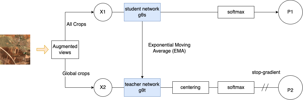
Figure 1: DINO: the self-supervised contrastive algorithm with knowledge distillation. It is the basic structure of both DINO-TP and DINO-MC. For DINO-TP, we use three temporal views to generate global crops and multi-sizes local crops as the input to do positive contrastive representation learning. For DINO-MC, we generate global and local crops from one imagery, then apply two different augmentations to global views and multi-sizes local views, respectively, to get the input of teacher and student network.

2 Related Work

2.1 Contrastive Self-supervised Learning.

The self-supervised pre-training aims to learn a general features which can generalise well to different downstream tasks. As a branch of self-supervised methods, contrastive learning has recently gained attention and shown promise in performance. It learns feature representations by maximizing the similarity of two positive instances and the distance between positive and negative instances. In generative and discriminative models, the encoder is trained to learn feature representations by optimizing the loss function calculated on the ground truth and the prediction, while the loss of contrastive model is calculated in the latent space [45].

Instance discrimination [15] is a simple but effective pretext task. It is widely used in contrastive learning which sets augmented views of the same input as positive samples and different instances as negative samples, and then trains the model to keep positive pairs close and negative pairs far in the representation space [15, 48, 40, 34]. [20] proposes Momentum Contrast model (MoCo-V1) with a momentum encoder to effectively maintain multiple negative samples for representation learning. SimCLR [7] employs very large batch sizes instead of momentum encoders, and provides experimental results on $10$ forms of data augmentation. Inspired by SimCLR, MoCo-V1 is extended to MoCo-V2 [9], and then MoCo-V3 [10] is proposed by applying ViT as the backbone.

Clustering method is another line of contrastive learning, which demands no precise indication from the inputs [4]. [5] introduces a contrasting cluster assignment that learns features by Swapping Assignments between multiple Views of the same image (SwAV). SwAV is easily applicable to different sizes of datasets since it employs clustering instead of pairwise comparisons. Furthermore, [5] proposes a new data augmentation named multi-crop to increase the instances without drastically additional memory and computation. Specifically, when doing multi-crop, images will be cropped to a collection of views with lower resolutions instead of the full-resolution views. Multi-crop shows both efficiency and effectiveness since several self-supervised models [4, 1, 7] perform well with it.

Knowledge distillation can be used in contrastive learning for feature extraction without separating between images [6]. [19] proposes Bootstrap Your Own Latent (BYOL) based on the online and target networks whose weights are updated with each other. BYOL experiments with ResNet of different sizes. Inspired by BYOL, [6] explores the further synergy between SSL and different backbones, especially ViTs, and proposes a simple form of self-distillation with no labels (DINO). DINO uses the same two networks architecture as BYOL but with different loss function and backbone models. When pre-trained on ImageNet [33], DINO achieves better linear and KNN probing evaluation results than other self-supervised methods with fewer computation resources [19, 5, 6].

2.2 Self-supervised Learning in Remote Sensing.

[38] experiments with self-supervised models on different pretext tasks, including image inpainting [31], context prediction [13], and instance discrimination [48] on remote sensing imagery tasks. [43] proposes to learn practical representations from satellite imagery by reconstructing the visible colors (RGB) from its high-dimensionality spectral bands (Spectral). [3] explores the application of contrastive representation learning to large-scale satellite image datasets. [25] proposes the seasonal contrast (SeCo) method, which significantly improves the performance of MoCo-V2 on three remote sensing tasks. Similar to [3], SeCo utilizes temporal information from remote sensing images to set two kinds of experiments MoCo-V2 with TP and SeCo. MoCo-V2 with TP is a positive temporal contrast, which regards the temporal views as the positive instances and trains models match their representations allowing the model to learn essential features that do not change over time. While SeCo is a negative temporal contrastive model regarding temporal views as the negative instances to capture the changes or differences because of the time changing. [44] uses Swin Transformer as the backbone of DINO and applies it to remote sensing imagery tasks. DINO-MM [46] extends DINO by combining synthetic-aperture radar (SAR) and multispectral (optical) images and is applied to BigEarthNet land use classification task.

Existing studies have demonstrated the value and feasibility of self-supervised models for practical applications in remote sensing image tasks. However, the potential of SSL in remote sensing has not been fully unlocked. Our work targets to bridge this gap and extend existing self-supervised model by generating more effective contrastive instances.

3 Method

Our work is mainly based on a contrastive self-supervised model DINO, which has been applied to both natural and remote sensing imagery [6, 46, 47]. We aim to learn useful, transferable features for remote sensing imagery by exploring positive temporal contrastive self-supervised model DINO-TP (Sec. 3.1) and introducing a self-supervised learning method DINO-MC (Sec. 3.2). In addition, we also experiment with the feature extraction ability of different backbones in SSL.

3.1 DINO-TP

Architecture Fig. 1 shows the model structure. The student and teacher networks in DINO are two neural networks with the same architecture $g$ but different weights $\theta_{t}$ and $\theta_{s}$. Two sets of augmented views $x_{1}$ and $x_{2}$ are generated from the same image. The student network receives both global and local crops as inputs, whereas the teacher network only receives global crops. Specifically, the global view covers the majority of the initial image and the local view only contains a small portion of it. In this way, the model is trained to match the individual local views to global views in the feature space.

Rather than a pre-trained and frozen teacher network used in previous study [17, 8], DINO dynamically updates the teacher weights by using EMA on student weights

$$\theta_{t}\leftarrow\theta_{t}\lambda+(1-\theta_{s})$$ (1)

, where $\theta_{t}$ is the current weight of the teacher network and $\theta_{s}$ is the current weight of the student network. The $\lambda$ values adhere to a cosine schedule between $0.996$ and $1$, indicating that the teacher network is less dependent on the present student and more dependent on the integration of the student network in each round; hence, the weights are updated slowly.

DINO uses centering and sharpening to prevent model collapse. Centering is adding a bias term $c$ to the features of the output of the teacher model, i.e.,

$$g_{t}(x)=g_{t}(x)+c$$ (2)

As Eq. 3 shown, the bias term $c$ is dynamically updated by the EMA, where $m>0$ denotes the update rate and $B$ is the batch size.

$$c\leftarrow mc+(1-m)\frac{1}{B}\sum_{i=1}^{B}g\theta_{t}(x_{i})$$ (3)

DINO achieves sharpening by performing softmax normalization using low temperature in the teacher network to avoid consistent distribution. The teacher network in DINO consistently performs better than the student network during pre-training, so it is used as the feature extractor in downstream tasks after pre-training [6].

Figure 2: The process of handling temporal views of contrastive learning in DINO-TP. We randomly select three temporal views of the same location and augment them to obtain global and local crops, which is the input of the teacher and student network. Different temporal views of the same location in DINO-TP are considered as positive examples, and we train the model to match their representations in the feature space.

Temporal Contrastive This work performs self-supervised pre-training on SeCo-100K [25] to exploit temporal information in representation learning. SeCo-100K is an unlabeled remote sensing imagery dataset with 100K instances, and each instance is composed of five different temporal views of the same location. In DINO-TP, we regard the temporal views of the same location as the positive instances, i.e., we pre-train the teacher and student networks to match temporal views in the feature space. The exact process is as follows. In the pre-training phase, we randomly select three temporal views and name them as $t_{0},t_{1},t_{2}$. As shown in Fig. 2, $t_{1},t_{2}$ can be regarded as the temporal augmentation views of $t_{0}$. The temporal image $t_{0}$ is directly used as $q$ to generate $6$ local crops of various sizes, including $184^{2},164^{2},144^{2},124^{2},104^{2}$ and $84^{2}$. After applying color jittering, grayscale, and Gaussian blur to each of the three temporal perspectives, we acquire $k_{0},k_{1},k_{2}$ views. We scale $k_{0},k_{1},k_{2}$ within a specific range and resize them into $224^{2}$ to get three global crops, which are used as the input of the teacher network. In prior work, different techniques are paired with different crop scaling ranges. SwAV uses $(0.05,0.14),(0.14,1)$ [5] and DINO chooses $(0.05,0.32),(0.32,1)$ [6]. This study follows DINO and uses $(0.05,0.32),(0.32,1)$ as the scaling range for local crops and global crops. Following this method, DINO-TP not only learns the relationship between the whole and the pieces of the image, but also discovers the correlation between various temporal perspectives.

3.2 DINO-MC

The structure of DINO-MC is nearly identical to DINO-TP. Intuitively, DINO-MC can be regarded as DINO with different multi-crop and color transformation augmentations, and as DINO-TP without temporal views. In our work, we change the cropping strategy for local crops in DINO to create a more challenging pretext task. We use multi-sized crops instead of the fixed-size local crops used in DINO. Keeping the number of global and local crops same as DINO, DINO-MC outperforms DINO on both linear and KNN probing as well as end-to-end evaluation on multiple downstream tasks. Color-related pretext tasks have been proven to be effective in many image tasks in the field of remote sensing [50, 43, 2]. This is due to the strong connection between color and semantics. Therefore, we set two strategies of color transformations for global and local crops respectively. The global views are augmented by random color jittering and GaussianBlur. The local views are augmented by random color jittering, random grayscale shifting, and random Gaussian blur all together. Random color jittering can change the brightness, contrast, saturation and hue of the image with a specific probability within a certain range. It is a commonly used color transformation method because it can simulate the effect of shooting in different lighting environments and other real-world shooting situations. Random grayscale converts an image into a grayscale image randomly. This enhancement method can reduce the impact of color, which is beneficial for some specific application scenarios, and can learn aspects other than color properties. We use different cropping strategy and different settings for color transformation. Our strategy is simple but effective, and the experiments verify that DINO-MC outperforms DINO on both linear probing and end-to-end fine-tuning on three downstream tasks (classification and change detection).

4 Experiments

In this study, we evaluate the features learned from the self-supervised pre-training on two downstream tasks: a land use classification on EuroSAT [22] and a change detection task on OSCD [12].

Self-supervised Pre-training We adopt and extend DINO for doing experiments since it is not only flexible and effective but also greatly declines the computational requirements. The models are pre-trained on SeCo-100K dataset [25], which is collected from Sentinel-2 [16] for self-supervised representation learning. It is an unlabeled remote sensing dataset containing 100K instances from different locations around the world, each consisting of five temporal views taken from the same location. In the pre-training phase, two distinct sets of temporal views of the same region are supplied to the student and teacher networks, respectively, then the self-supervised model matches these views in feature space to generate representations that do not vary over time. In DINO-MC and DINO-TP, the scaling range of multi-crop is $(0.05,0.32)$ for local crops and $(0.32,1)$ for global crops. Our self-supervised models, pretrained on 100k images over 300 epochs, is compared against several baselines, including DINO, MoCo-V2, and SeCo, on three different remote sensing downstream tasks, while using less overall computation than the current state of the art (SeCo-1M).

4.1 DINO with Different Backbones

Being the backbone of DINO, ViT is superior to ResNet [6]. In this work, there are four different networks applied as the backbone of DINO, DINO-TP, and DINO-MC, including ViT, Swin Transformer, ResNet, and WRN.

ViT preserves the Transformer structure used in NLP as much as possible and performs very well in computer vision tasks [14]. The input of transformer encoder is the embedding formed by adding the patch embedding with the position encoding. The transformer encoder of ViT consists mainly of layer normalization (LN) which is applied before each block, multi-head attention, and multi-layer perceptron block (MLP).

Inspired by ViT, Swin Transformer is proposed with a hierarchical transformer, which computes representation with both regular and shifted windows to capture features from different levels and resolutions.

A deep residual learning framework (ResNet) is proposed to overcome the degradation issue by [21]. They add shortcut connections to transmit the information of shallow layers directly to the deeper layers of the neural network and require no additional computation. With this mechanism, the residual net is deepened to $152$ layers and achieves state-of-the-art results in multiple computer vision tasks. Furthermore, with the development of self-supervised representation learning, ResNet also becomes an effective backbone widely used in multiple self-supervised architectures [7, 19, 29, 39, 26].

WRN [49] is proposed to improve the performance of ResNet by increase the width of the residual block, i.e., widening the convolutional layers. When the same number of parameters are utilized, wide residual block can get superior outcomes with less training time compared to the original residual block. WRN adds a widening factor to a block denoted by $k$, and the initial residual block can be represented as $k=1$. Although the parameters numbers and computational complexity are quadratic in $k$, this method is more effective than expanding the number of layers in ResNet since large tensors are able to make better use of the parallel-computing ability of GPUs [49]. WRN is proved to achieve new state-of-the-art results in a supervised manner in terms of classification F1-Score and training efficiency [30]. Therefore, this project intends to employ it with a self-supervised training framework.

Implementation Details There are different sizes of ViT models, and we use ViT-small as the backbone model and implement it following DINO. In the experiments, we load different backbones as the teacher and student network without pre-trained weights. WRN-50-2 has similar structure to ResNet, with the exception of the bottleneck number of channels, which is twice as large in each block. We follow the recommendation from DINO to use AdamW optimizer. We use cross-entropy as the loss function to calculate the distance between feature representations output by two networks. We evaluate the learned representations by applying KNN and linear probing on EuroSAT land use classification task.

Quantitative Results In order to evaluate the representations independently, the feature extraction model is frozen and only linear and KNN classifiers are trained on EuroSAT land use classification task. The results are shown in Tab. 1. From the table, DINO-MC performs better than both DINO and DINO-TP when using ViT-samll, WRN-50-2, and ResNet-50 backbones. DINO-MC with WRN-50-2 pre-trained on 100K data is even 2.56% higher than the linear probing accuracy of SeCo pre-trained on 1 million data. Besides, DINO-MC with ViT-samll has 2.59% higher accuracy than DINO with ViT-samll which indicates the effectiveness of our strategy. In comparison to the other three backbones, Swin-tiny performs less well. One possible reason could be that the model size of Swin-tiny is much smaller than the other three models. Another interesting observation is that the DINO-TP performs worse with two convnets than the DINO, but better with two transformer models. Among the different self-supervised models, ViT-small and Swin-tiny performed more consistently than ResNet-50 and WRN-50-2. Overall, DINO-MC is particularly effective.

Model	Arch	#images	KNN	Linear
MoCo-V2	ResNet-50	1M	-	83.72
SeCo-1M	ResNet-50	1M	-	93.14
DINO	ResNet-50	100K	90.09	89.65
DINO-MC	ResNet-50	100K	93.94	95.59
DINO-TP	ResNet-50	100K	79.05	86.70
DINO	WRN-50-2	100K	92.74	91.65
DINO-MC	WRN-50-2	100K	94.65	95.70
DINO-TP	WRN-50-2	100K	86.37	88.15
DINO	ViT-small	100K	93.35	91.50
DINO-MC	ViT-small	100K	93.41	94.09
DINO-TP	ViT-small	100K	93.15	93.89
DINO	Swin-tiny	100K	92.15	86.87
DINO-MC	Swin-tiny	100K	93.22	90.54
DINO-TP	Swin-tiny	100K	92.83	91.94

Table 1: Linear and KNN probing classification on EuroSAT. We evaluate our models with different backbones on EuroSAT and record the top-1 accuracy of KNN and linear probing on the validation set. MoCo-V2 [9] and SeCo-1M [25] are pre-trained on SeCo-1M dataset, and their linear probing results on EuroSAT are from SeCo [25]. Other listed models are pre-trained on SeCo-100K dataset with only 10% images of SeCo-1M.

4.2 Land Use Classification on EuroSAT

EuroSAT is a widely used benchmark dataset for remote sensing land use classification tasks. It is used for representation evaluation in this study, allowing the results of models based on it to be easily compared to those of other models. The dataset, which collects 27,000 remote sensing images from the Sentinel-2 satellite, is divided into 21,600 and 5,400 images for training and evaluation in the experiment, respectively.

Implementation Details The pre-trained backbone models in self-supervised learning are evaluated as feature extractors in this land use classification downstream task. Based on the pre-trained backbone models, we add a fully-connected layer as the classifier to output the classification results. Both the feature extractor and the classifier are fine-tuning on this supervised classification task. We train the models for around 200 epochs with a batch size of 32. The learning rate is $1e-3$ or $3e-3$ for different models. We use the CosineAnnealingLR scheduler to update the learning rate. Same as SeCo [25], we use SGD optimizer without weight decay to update weights.

Quantitative Results Tab. 2 compares our pre-trained models against three supervised baseline models on EuroSAT land use classification task. DINO-MC with WRN-50-2 achieves similar results to the three supervised models, in particular, it was pre-trained on only 100K images, while the three supervised models were pre-trained on 1M images. This further confirms the effectiveness of the representations learned by DINO-MC.

Model	Backbone	Accuracy
Supervised	WRN-50-2	98.72
Supervised	ResNet-50	98.78
Supervised	ViT-base	98.83
DINO	ViT-small	97.98
DINO-MC	ViT-small	98.15
DINO-MC	Swin-tiny	98.43
DINO-MC	ResNet-50	98.69
DINO-MC	WRN-50-2	98.78

Table 2: End-to-end accuracy results on EuroSAT land use classification task. The three supervised models listed are pre-trained on ImageNet-1K [33], and we load and fine-tune them on EuroSAT. While DINO and DINO-MC are only pre-trained on SeCo-100K dataset, which has only 10% the number of images of ImageNet-1K.

4.3 Land Use Classification on BigEarthNet

BigEarthNet [36] is a widely used benchmark dataset for land use classification task, containing a total of 590,326 images. This paper uses BigEarthNet-S2 [36], which collects remote sensing images from Sentinel-2 only, and each image is annotated by multiple land use categories. The dataset provides 12 spectral bands for each image and a JSON file with its multi-labels and metadata information. Following SeCo [25], we employ a new nomenclature of 19 classes introduced in [37], and around $12\%$ of the patches that are totally masked by seasonal snow, clouds, or cloud shadows are eliminated in this experiment. We used the training/validation splitting strategy suggested by [28] with 311,667 instances for training and 103,944 images for validation.

Implementation Details We add a linear classification layer on top of the backbone model as the output layer and then fine-tune it on 10% and 100% BigEarthNet, respectively, to evaluate the features learned by the self-supervised models. In this experiment, the Adam and AdamW optimizer with default hyper-parameters are used to update the weights of the models. Identical to SeCo, we set the learning rate to $1e-5$ and scale it down by ten in epochs of 60% and 80%, respectively. We use the MultiLabelSoftMarginLoss as the loss function, which allows assigning a different number of target classes to each sample.

Quantitative Results Tab. 3 provides the results of each pre-trained model in the end-to-end BigEarthNet classification task. We measure the performance of each model by mean average precision (MAP). When fine-tuned on the 10% BigEarthNet, DINO-MC outperforms SeCo-100K with the same backbone. Besides, DINO-MC with ViT-small achieves 1.65% higher MAP than with ResNet-50, 2.48% higher MAP than SeCo-100K, and even 1.58% higher MAP than SeCo-1M. The performance of DINO-MC with each of the four backbone models exceeds that of SeCo-100K, and even outperforms SeCo-1M except for ResNet-50.

When fine-tuned on the whole BigEarthNet, DINO-MC achieves comparable result to SeCo-100K with the same backbone. Interestingly, DINO-MC with Swin-tiny achieves 1.89% higher MAP than with ResNet-50, 1.63% higher MAP than SeCo-100K, and 0.94% higher than SeCo-1M. The results demonstrate that the representations learned by DINO-MC can generalize well on the multi-label classification task on BigEarthNet.

Model	Backbone	Param.	10%	100%
SeCo-100K	ResNet-50	23M	81.72	87.12
SeCo-1M	ResNet-50	23M	82.62	87.81
DINO	ResNet-50	23M	79.67	85.38
DINO-TP	ResNet-50	23M	80.10	85.20
DINO-MC	ResNet-50	23M	82.55	86.86
DINO-MC	WRN-50-2	69M	82.67	87.22
DINO-MC	Swin-tiny	28M	83.84	88.75
DINO-MC	ViT-small	21M	84.20	88.69

Table 3: Mean average precision (MAP) results on BigEarthNet-S2 land use classification. We use the same train/validation splits as SeCo [25]. The comparison is done by fine-tuning on 10% and 100% training data and evaluating on all validation dataset with different self-supervised models and backbones. SeCo-100K and SeCo-1M represent SeCo pre-trained on SeCo-100K and SeCo-1M, respectively, and their results listed are from [25]. DINO, DINO-MC, and DINO-TP are pre-trained on SeCo-100K only.

4.4 Change Detection on OSCD

Model	Backbone	Pre.	Rec.	F1
Supervised	ResNet-50	56.49	43.63	48.61
Supervised	WRN-50-2	53.76	47.11	49.72
PatchSSL (21M param.)		40.44	69.10	51.00
MoCo-V2	ResNet-50	64.49	30.94	40.71
SeCo-1M	ResNet-50	65.47	38.06	46.94
DINO	ResNet-50	57.37	44.21	49.53
DINO-MC	ResNet-50	51.94	54.04	52.46
DINO-TP	ResNet-50	51.10	49.03	49.74
DINO	WRN-50-2	53.58	52.28	52.41
DINO-MC	WRN-50-2	49.99	56.81	52.70
DINO-TP	WRN-50-2	55.77	47.30	50.61

Table 4: Fine-tuning accuracy results on OSCD change detection task. We adopt the same train/validation splits as SeCo [25]. Following SeCo, we freeze the pre-trained backbone and only update the weights of U-net [32]. Our WRN-50-2 and ResNet-50 models are pre-trained on 100K satellite images. The result of PatchSSL is from [11]. The listed MoCo-V2 [9] and SeCo-1M are pre-trained on 1M satellite images and are results provided by [25].

(a) Image 1
(Lasvegas)

(b) Image 2
(Lasvegas)

(c) Mask
(Ground truth)

(d) SeCo-1M
F1=84.25

(e) DINO
F1=86.83

(f) DINO-TP
F1=88.60

(g) DINO-MC
F1=86.69

(h) Image 1
(Dubai)

(i) Image 2
(Dubai)

(j) Mask
(Ground truth)

(k) SeCo-1M
F1=61.89

(l) DINO
F1=65.40

(m) DINO-TP
F1=59.64

(n) DINO-MC
F1=68.42

Figure 3: Same as SeCo [25], our visualization is based on two instances of ’Losvegas’ and ’Dubai’ from the OSCD change detection dataset. SeCo-1M is SeCo model pre-trained on SeCo-1M dataset, while DINO, DINO-TP, and DINO-MC are pre-trained on only SeCo-100K. We visualize the outputs of DINO-TP and DINO-MC for comparison with DINO and SeCo. We present results on the same images as SeCo for comparison and the two outputs of SeCo is from [25]. We also provide F1 score for each output on the bottom of output image.

The Onera Satellite Change Detection (OSCD) is a benchmark dataset of which the images are collected from Sentinel-2 satellites. It focuses primarily on urban growth and disregards natural changes [12]. Change detection is a fundamental problem in the field of earth observation image analysis. The input is a pair of images captured at the same location, while the label is a mask map highlighting the change parts. It is a binary classification task in which labels are assigned to each pixel based on a series of images sampled at different times: change (positive) or no change (negative). The results are measured by F1 Score, precision and recall.

Implementation Details The OSCD dataset is divided into fourteen and ten pairs for training and validation separately, as recommended by prior research [12, 25]. In addition, the categories of change and unchanged in this dataset are unbalanced due to the property of the task. We use the same U-net architecture as SeCo for the change detection task, which employ the pre-trained backbone models to extract features as the encoder in the U-net. We apply the pre-trained WRN-50-2 and ResNet-50 backbone models as the encoder and select the first convolution layer, and Layer 1 to 4 as the copy and cropping layers. As for the decoder module, it is constructed to rebuild an image with the same width and height as the input. And the input and output sizes of its layers are set according to the input and output of the specific encoder layers, in order to concatenate them in the direction of the channel. Upsampling here is achieved by interpolate function, which can be understood simply as a technology to increase the resolution of the output. The last layer of the U-net is a $1\times 1$ convolutional layer, which is used to map the channel of the feature vector to the number of output classes. During fine-tuning, in order to avoid overfitting, only the U-net weights are updated. In this task, the pre-trained WRN are fine-tuned with a batch size of $32$ and learning rate of $0.0006$. The loss function used is $BCEWithLogitsLoss+SoftDiceLoss$

Quantitative Results Tab. 4 provides the results of DINO, DINO-MC, and DINO-TC with ResNet-50 and WRN-50-2 respectively, compared against some supervised and self-supervised baselines on OSCD dataset. The F1 score of DINO-MC with ResNet-50 is $5.52\%$ higher than that of SeCo and almost $3\%$ higher than that of DINO. When using WRN-50-2 as the backbone, the F1 score of DINO-MC is $5.76\%$ higher than that of SeCo and similar with DINO. It is no surprise that DINO-TP does not perform as well as DINO and DINO-MC, because DINO-TP receives images of the same location taken at different times as positive instances, so it aims to learn features that do not change over time, which is not very suitable for change detection task [25]. In the results of OSCD task, the backbones pre-trained in DINO-MC can capture the subtle differences of image changes over time after a simple fine-tuning on the change detection dataset, which indicates that DINO-MC is able to learn general and effective features using only very simple data augmentation methods.

Qualitative Results Fig. 3 gives the visualization masks of DINO-MC on OSCD task. To do comparison to SeCo, we select two identical examples from the OSCD validation set. The masks generated by DINO-MC outperform SeCo-1M since they cover more changed pixels without excessive false predictions. We observe that the performance of DINO-TP on OSCD task is unstable since it achieves particularly high F1 score on the first instance, which is $4.35$ higher than SeCo-1M, but much lower in the second one, which is $2.25$ lower than SeCo-1M. Although positive temporal contrast used in DINO-TP has been proved to be undesirable for change detection task [25], the performance of DINO-TP is comparable to SeCo-1M when evaluated on the whole validation set.

5 Conclusions

In this work, we introduce DINO-TP and DINO-MC, which extend DINO in two ways: (1) DINO-TP employs a positive temporal contrast strategy and (2) DINO-MC utilizes a new cropping strategy and color transformations for local views. Experimental results of KNN and linear probing evaluation on EuroSAT demonstrate the effectiveness of our cropping strategy, as well as the unstable performance of the positive temporal contrast on remote sensing imagery. We evaluate and compare our models with some self-supervised and supervised baselines on three remote sensing tasks. The results of three end-to-end tasks indicate the superiority and efficiency of DINO-MC over the existing state-of-the-art models.

Acknowledgement This research was undertaken using the LIEF HPC-GPGPU Facility hosted at the University of Melbourne. This Facility was established with the assistance of LIEF Grant LE170100200.

References

- [1] Yuki Markus Asano, Christian Rupprecht, and Andrea Vedaldi. Self-labelling via simultaneous clustering and representation learning. arXiv preprint arXiv:1911.05371, 2019.
- [2] Mahmoud Assran, Mathilde Caron, Ishan Misra, Piotr Bojanowski, Florian Bordes, Pascal Vincent, Armand Joulin, Michael Rabbat, and Nicolas Ballas. Masked siamese networks for label-efficient learning. arXiv preprint arXiv:2204.07141, 2022.
- [3] Kumar Ayush, Burak Uzkent, Chenlin Meng, Kumar Tanmay, Marshall Burke, David Lobell, and Stefano Ermon. Geography-aware self-supervised learning. In Proceedings of the IEEE/CVF International Conference on Computer Vision, pages 10181–10190, 2021.
- [4] Mathilde Caron, Piotr Bojanowski, Armand Joulin, and Matthijs Douze. Deep clustering for unsupervised learning of visual features. In Proceedings of the European conference on computer vision (ECCV), pages 132–149, 2018.
- [5] Mathilde Caron, Ishan Misra, Julien Mairal, Priya Goyal, Piotr Bojanowski, and Armand Joulin. Unsupervised learning of visual features by contrasting cluster assignments. Advances in Neural Information Processing Systems, 33:9912–9924, 2020.
- [6] Mathilde Caron, Hugo Touvron, Ishan Misra, Hervé Jégou, Julien Mairal, Piotr Bojanowski, and Armand Joulin. Emerging properties in self-supervised vision transformers. In Proceedings of the IEEE/CVF International Conference on Computer Vision, pages 9650–9660, 2021.
- [7] Ting Chen, Simon Kornblith, Mohammad Norouzi, and Geoffrey Hinton. A simple framework for contrastive learning of visual representations. In International conference on machine learning, pages 1597–1607. PMLR, 2020.
- [8] Ting Chen, Simon Kornblith, Kevin Swersky, Mohammad Norouzi, and Geoffrey E Hinton. Big self-supervised models are strong semi-supervised learners. Advances in neural information processing systems, 33:22243–22255, 2020.
- [9] Xinlei Chen, Haoqi Fan, Ross Girshick, and Kaiming He. Improved baselines with momentum contrastive learning. arXiv preprint arXiv:2003.04297, 2020.
- [10] Xinlei Chen, Saining Xie, and Kaiming He. An empirical study of training self-supervised vision transformers. In Proceedings of the IEEE/CVF International Conference on Computer Vision, pages 9640–9649, 2021.
- [11] Yuxing Chen and Lorenzo Bruzzone. Self-supervised remote sensing images change detection at pixel-level. arXiv preprint arXiv:2105.08501, 2021.
- [12] Rodrigo Caye Daudt, Bertr Le Saux, Alexandre Boulch, and Yann Gousseau. Urban change detection for multispectral earth observation using convolutional neural networks. In IGARSS 2018-2018 IEEE International Geoscience and Remote Sensing Symposium, pages 2115–2118. Ieee, 2018.
- [13] Carl Doersch, Abhinav Gupta, and Alexei A Efros. Unsupervised visual representation learning by context prediction. In Proceedings of the IEEE international conference on computer vision, pages 1422–1430, 2015.
- [14] Alexey Dosovitskiy, Lucas Beyer, Alexander Kolesnikov, Dirk Weissenborn, Xiaohua Zhai, Thomas Unterthiner, Mostafa Dehghani, Matthias Minderer, Georg Heigold, Sylvain Gelly, et al. An image is worth 16x16 words: Transformers for image recognition at scale. arXiv preprint arXiv:2010.11929, 2020.
- [15] Alexey Dosovitskiy, Jost Tobias Springenberg, Martin Riedmiller, and Thomas Brox. Discriminative unsupervised feature learning with convolutional neural networks. Advances in neural information processing systems, 27, 2014.
- [16] Matthias Drusch, Umberto Del Bello, Sébastien Carlier, Olivier Colin, Veronica Fernandez, Ferran Gascon, Bianca Hoersch, Claudia Isola, Paolo Laberinti, Philippe Martimort, et al. Sentinel-2: Esa’s optical high-resolution mission for gmes operational services. Remote sensing of Environment, 120:25–36, 2012.
- [17] Zhiyuan Fang, Jianfeng Wang, Lijuan Wang, Lei Zhang, Yezhou Yang, and Zicheng Liu. Seed: Self-supervised distillation for visual representation. arXiv preprint arXiv:2101.04731, 2021.
- [18] M. K. Firozjaei, A. Sedighi, H. K. Firozjaei, M. Kiavarz, and Ska Panah. A historical and future impact assessment of mining activities on surface biophysical characteristics change: A remote sensing-based approach. Ecological Indicators, 122(2021), 2021.
- [19] Jean-Bastien Grill, Florian Strub, Florent Altché, Corentin Tallec, Pierre Richemond, Elena Buchatskaya, Carl Doersch, Bernardo Avila Pires, Zhaohan Guo, Mohammad Gheshlaghi Azar, et al. Bootstrap your own latent-a new approach to self-supervised learning. Advances in neural information processing systems, 33:21271–21284, 2020.
- [20] Kaiming He, Haoqi Fan, Yuxin Wu, Saining Xie, and Ross Girshick. Momentum contrast for unsupervised visual representation learning. In Proceedings of the IEEE/CVF conference on computer vision and pattern recognition, pages 9729–9738, 2020.
- [21] Kaiming He, Xiangyu Zhang, Shaoqing Ren, and Jian Sun. Deep residual learning for image recognition. In Proceedings of the IEEE conference on computer vision and pattern recognition, pages 770–778, 2016.
- [22] Patrick Helber, Benjamin Bischke, Andreas Dengel, and Damian Borth. Eurosat: A novel dataset and deep learning benchmark for land use and land cover classification. IEEE Journal of Selected Topics in Applied Earth Observations and Remote Sensing, 12(7):2217–2226, 2019.
- [23] Geoffrey Hinton, Oriol Vinyals, and Jeff Dean. Distilling the knowledge in a neural network. arXiv preprint arXiv:1503.02531, 2015.
- [24] T. Kattenborn, J. Leitloff, F. Schiefer, and S. Hinz. Review on convolutional neural networks (cnn) in vegetation remote sensing. ISPRS Journal of Photogrammetry and Remote Sensing, 173:24–49, 2021.
- [25] Oscar Manas, Alexandre Lacoste, Xavier Giró-i Nieto, David Vazquez, and Pau Rodriguez. Seasonal contrast: Unsupervised pre-training from uncurated remote sensing data. In Proceedings of the IEEE/CVF International Conference on Computer Vision, pages 9414–9423, 2021.
- [26] Ishan Misra and Laurens van der Maaten. Self-supervised learning of pretext-invariant representations. In Proceedings of the IEEE/CVF Conference on Computer Vision and Pattern Recognition, pages 6707–6717, 2020.
- [27] Mulla and J. David. Twenty five years of remote sensing in precision agriculture: Key advances and remaining knowledge gaps. Biosystems Engineering, 114(4):358–371, 2013.
- [28] Maxim Neumann, Andre Susano Pinto, Xiaohua Zhai, and Neil Houlsby. In-domain representation learning for remote sensing. arXiv preprint arXiv:1911.06721, 2019.
- [29] Aaron van den Oord, Yazhe Li, and Oriol Vinyals. Representation learning with contrastive predictive coding. arXiv preprint arXiv:1807.03748, 2018.
- [30] Ioannis Papoutsis, Nikolaos-Ioannis Bountos, Angelos Zavras, Dimitrios Michail, and Christos Tryfonopoulos. Efficient deep learning models for land cover image classification. arXiv preprint arXiv:2111.09451, 2021.
- [31] Deepak Pathak, Philipp Krahenbuhl, Jeff Donahue, Trevor Darrell, and Alexei A Efros. Context encoders: Feature learning by inpainting. In Proceedings of the IEEE conference on computer vision and pattern recognition, pages 2536–2544, 2016.
- [32] Olaf Ronneberger, Philipp Fischer, and Thomas Brox. U-net: Convolutional networks for biomedical image segmentation. In International Conference on Medical image computing and computer-assisted intervention, pages 234–241. Springer, 2015.
- [33] Olga Russakovsky, Jia Deng, Hao Su, Jonathan Krause, Sanjeev Satheesh, Sean Ma, Zhiheng Huang, Andrej Karpathy, Aditya Khosla, Michael Bernstein, et al. Imagenet large scale visual recognition challenge. International journal of computer vision, 115:211–252, 2015.
- [34] Sachith Seneviratne, Kerry A Nice, Jasper S Wijnands, Mark Stevenson, and Jason Thompson. Self-supervision. remote sensing and abstraction: Representation learning across 3 million locations. In 2021 Digital Image Computing: Techniques and Applications (DICTA), pages 01–08. IEEE, 2021.
- [35] Vladan Stojnic and Vladimir Risojevic. Self-supervised learning of remote sensing scene representations using contrastive multiview coding. In Proceedings of the IEEE/CVF Conference on Computer Vision and Pattern Recognition, pages 1182–1191, 2021.
- [36] Gencer Sumbul, Marcela Charfuelan, Begüm Demir, and Volker Markl. Bigearthnet: A large-scale benchmark archive for remote sensing image understanding. In IGARSS 2019-2019 IEEE International Geoscience and Remote Sensing Symposium, pages 5901–5904. IEEE, 2019.
- [37] Gencer Sumbul, Jian Kang, Tristan Kreuziger, Filipe Marcelino, Hugo Costa, Pedro Benevides, Mario Caetano, and Begüm Demir. Bigearthnet dataset with a new class-nomenclature for remote sensing image understanding. arXiv preprint arXiv:2001.06372, 2020.
- [38] Chao Tao, Ji Qi, Weipeng Lu, Hao Wang, and Haifeng Li. Remote sensing image scene classification with self-supervised paradigm under limited labeled samples. IEEE Geoscience and Remote Sensing Letters, 2020.
- [39] Yonglong Tian, Dilip Krishnan, and Phillip Isola. Contrastive multiview coding. In European conference on computer vision, pages 776–794. Springer, 2020.
- [40] Yonglong Tian, Chen Sun, Ben Poole, Dilip Krishnan, Cordelia Schmid, and Phillip Isola. What makes for good views for contrastive learning? Advances in Neural Information Processing Systems, 33:6827–6839, 2020.
- [41] Woody Turner, Sacha Spector, Ned Gardiner, Matthew Fladeland, Eleanor Sterling, and Marc Steininger. Remote sensing for biodiversity science and conservation. Trends in ecology & evolution, 18(6):306–314, 2003.
- [42] CJ Van Westen. Remote sensing for natural disaster management. International archives of photogrammetry and remote sensing, 33(B7/4; PART 7):1609–1617, 2000.
- [43] Stefano Vincenzi, Angelo Porrello, Pietro Buzzega, Marco Cipriano, Pietro Fronte, Roberto Cuccu, Carla Ippoliti, Annamaria Conte, and Simone Calderara. The color out of space: learning self-supervised representations for earth observation imagery. In 2020 25th International Conference on Pattern Recognition (ICPR), pages 3034–3041. IEEE, 2021.
- [44] Xuying Wang, Jiawei Zhu, Zhengliang Yan, Zhaoyang Zhang, Yunsheng Zhang, Yansheng Chen, and Haifeng Li. Last: Label-free self-distillation contrastive learning with transformer architecture for remote sensing image scene classification. IEEE Geoscience and Remote Sensing Letters, 19:1–5, 2022.
- [45] Yi Wang, Conrad M Albrecht, Nassim Ait Ali Braham, Lichao Mou, and Xiao Xiang Zhu. Self-supervised learning in remote sensing: A review. arXiv preprint arXiv:2206.13188, 2022.
- [46] Yi Wang, Conrad M Albrecht, and Xiao Xiang Zhu. Self-supervised vision transformers for joint sar-optical representation learning. In IGARSS 2022-2022 IEEE International Geoscience and Remote Sensing Symposium, pages 139–142. IEEE, 2022.
- [47] Yi Wang, Nassim Ait Ali Braham, Zhitong Xiong, Chenying Liu, Conrad M Albrecht, and Xiao Xiang Zhu. Ssl4eo-s12: A large-scale multi-modal, multi-temporal dataset for self-supervised learning in earth observation. arXiv preprint arXiv:2211.07044, 2022.
- [48] Zhirong Wu, Yuanjun Xiong, Stella X Yu, and Dahua Lin. Unsupervised feature learning via non-parametric instance discrimination. In Proceedings of the IEEE conference on computer vision and pattern recognition, pages 3733–3742, 2018.
- [49] Sergey Zagoruyko and Nikos Komodakis. Wide residual networks. arXiv preprint arXiv:1605.07146, 2016.
- [50] Richard Zhang, Phillip Isola, and Alexei A Efros. Colorful image colorization. In European conference on computer vision, pages 649–666. Springer, 2016.