Abstract Voronoi-like Graphs: Extending Delaunay’s Theorem and Applications

Abstract

Any system of bisectors (in the sense of abstract Voronoi diagrams) defines an arrangement of simple curves in the plane. We define Voronoi-like graphs on such an arrangement, which are graphs whose vertices are locally Voronoi. A vertex $v$ is called locally Voronoi, if $v$ and its incident edges appear in the Voronoi diagram of three sites. In a so-called admissible bisector system, where Voronoi regions are connected and cover the plane, we prove that any Voronoi-like graph is indeed an abstract Voronoi diagram. The result can be seen as an abstract dual version of Delaunay’s theorem on (locally) empty circles.

Further, we define Voronoi-like cycles in an admissible bisector system, and show that the Voronoi-like graph induced by such a cycle $C$ is a unique tree (or a forest, if $C$ is unbounded). In the special case where $C$ is the boundary of an abstract Voronoi region, the induced Voronoi-like graph can be computed in expected linear time following the technique of [Junginger and Papadopoulou SOCG’18]. Otherwise, within the same time, the algorithm constructs the Voronoi-like graph of a cycle $C^{\prime}$ on the same set (or subset) of sites, which may equal $C$ or be enclosed by $C$. Overall, the technique computes abstract Voronoi (or Voronoi-like) trees and forests in linear expected time, given the order of their leaves along a Voronoi-like cycle. We show a direct application in updating a constraint Delaunay triangulation in linear expected time, after the insertion of a new segment constraint, simplifying upon the result of [Shewchuk and Brown CGTA 2015].

1 Introduction

Delaunay’s theorem [6] is a well-known cornerstone in Computational Geometry: given a set of points, a triangulation is globally Delaunay if and only if it is locally Delaunay. A triangulation edge is called locally Delaunay if it is incident to only one triangle, or it is incident to two triangles, and appears in the Delaunay triangulation of the four related vertices. The Voronoi diagram and the Delaunay triangulation of a point set are dual to each other. These two highly influential and versatile structures are often used and computed interchangeably; see the book of Aurenhammeret al.[2] for extensive information.

Let us pose the following question: how does Delaunay’s theorem extend to Voronoi diagrams of generalized (not necessarily point) sites? We are interested in simple geometric objects such as line segments, polygons, disks, or point clusters, as they often appear in application areas, and answering this question is intimately related to efficient construction algorithms for Voronoi diagrams (or their duals) on these objects. Here we consider this question in the framework of abstract Voronoi diagrams [11] so that we can simultaneously answer it for various concrete and fundamental cases under their umbrella.

Although Voronoi diagrams and Delaunay triangulations of point sites have been widely used in many fields of science, being available in most software libraries of commonly used programming languages, practice has not been the same for their counterparts of simple geometric objects. In fact it is surprising that certain related questions may have remained open or non-optimally solved. Edelsbrunner and Seidel [7] defined Voronoi diagrams as lower envelopes of distance functions in a space one dimension higher, making a powerful link to arrangements, which made their rich combinatorial and algorithmic results applicable, e.g.,  [14]. However, there are different levels of difficulty concerning arrangements of planes versus more general surfaces, which play a role, especially in practice.

In this paper we define Voronoi-like graphs based on local information, inspired by Delaunay’s theorem. Following the framework of abstract Voronoi diagrams (AVDs) [11], let $S$ be a set of $n$ abstract sites (a set of indices) and $\mathcal{J}$ be their underlying system of bisectors, which satisfies some simple combinatorial properties (see Sections 2, 3). Consider a graph $G$ on the arrangement of the bisector system possibly truncated within a simply connected domain $D$. The vertices of $G$ are vertices of the bisector arrangement, its leaves lie on the boundary $\partial D$, and the edges are maximal bisector arcs connecting pairs of vertices. A vertex $v$ in $G$ is called locally Voronoi, if $v$ and its incident edges within a small neighborhood around $v$ appear in the Voronoi diagram of the three sites defining $v$ (Def. 3.1), see Figure 4. The graph $G$ is called Voronoi-like, if its vertices (other than its leaves on $\partial D$) are locally Voronoi vertices (Def. 3.2), see Figure 5. If the graph $G$ is a simple cycle on the arrangement of bisectors related to one site $p$ and its vertices are locally Voronoi of degree 2, then it is called a Voronoi-like cycle, for brevity a site-cycle (Def. 3.9).

A major difference between points in the Euclidean plane, versus non-points, such as line segments, disks, or AVDs, can be immediately pointed out: in the former case the bisector system is a line arrangement, while in the latter, the bisecting curves are not even pseudolines. On a line arrangement, it is not hard to see that a Voronoi-like graph coincides with the Voronoi diagram of the involved sites: any Voronoi-like cycle is a convex polygon, which is in fact a Voronoi region in the Voronoi diagram of a subset of sites. But in the arrangement of an abstract bisector system, many different Voronoi-like cycles can exist for the same set of sites (see, e.g., Figure 10). Whether a Voronoi-like graph corresponds to a Voronoi diagram is not immediately clear.

In this paper we show that a Voronoi-like graph on the arrangement of an abstract bisector system is as close as possible to being an abstract Voronoi diagram, subject to, perhaps, missing some faces (see Def. 3.3); if the graph misses no face, then it is a Voronoi diagram. Thus, in the classic AVD model [11], where abstract Voronoi regions are connected and cover the plane, any Voronoi-like graph is indeed an abstract Voronoi diagram. This result can be seen as an abstract dual version of Delaunay’s theorem.

Voronoi-like graphs (and their duals) can be very useful structures to hold partial Voronoi information, either when dealing with disconnected Voronoi regions, or when considering partial information concerning some region. Building a Voronoi-like graph of partial information may be far easier and faster than constructing the full diagram. In some cases the full diagram may even be undesirable, as in the example of Section 6 in updating a constrained Delaunay triangulation.

The term Voronoi-like diagram was first used, in a restricted sence, by Junginger and Papadopoulou [8], defining it as a tree (occasionally a forest) that subdivided a planar region enclosed by a so-called boundary curve defined on a subset of Voronoi edges. Their Voronoi-like diagram was then used as an intermediate structure to perform deletion in an abstract Voronoi diagram in linear expected time. In this paper the formulation of a Voronoi-like graph is entirely different; we nevertheless prove that the Voronoi-like diagram of [8] remains a special case of the one in this paper. We thus use the results of [8] when applicable, and extend them to Voronoi-like cycles in an admissible bisector system.

In the remainder of this section we consider an admissible bisector system $\mathcal{J}$ following the classic AVD model [11], where bisectors are unbounded simple curves and Voronoi regions are connected. To avoid issues with infinity, we asume a large Jordan curve $\Gamma$ (e.g, a circle) bounding the computation domain, which is large enough to enclose any bisector intersection. In the sequel, we list further results, which are obtained in this paper under this model.

We consider a Voronoi-like cycle $C$ on the arrangement of bisectors $\mathcal{J}_{p}\subseteq\mathcal{J}\cup\Gamma$, which are related to a site $p\in S$. Let $S_{C}\subseteq S\setminus\{p\}$ be the set of sites that (together with $p$) contribute to the bisector arcs in $C$. The cycle $C$ encodes a sequence of site occurrences from $S_{C}$. We define the Voronoi-like graph $\mathcal{V}_{l}(C)$, which can be thought as a Voronoi diagram of site occurrences, instead of sites, whose order is represented by $C$. We prove that $\mathcal{V}_{l}(C)$ is a tree, or a forest if $C$ is unbounded, and it exists for any Voronoi-like cycle $C$. The uniqueness of $\mathcal{V}_{l}(C)$ can be inferred from the results in [8]. The same properties can be extended to Voronoi-like graphs of cycles related to a set $P$ of $k$ sites.

We then consider the randomized incremental construction of [8], and apply it to a Voronoi-like cycle in linear expected time. If $C$ is the boundary of a Voronoi region then $\mathcal{V}_{l}(C)$, which is the part of the abstract Voronoi diagram $\mathcal{V}(S_{C})$, truncated by $C$, can be computed in expected linear time (this has been previously shown [8, 10]). Otherwise, within the same time, the Voronoi-like graph of a (possibly different) Voronoi-like cycle $C\textquoteright$, enclosed by $C$, is computed by essentially the same algorithm. We give conditions under which we can force the randomized algorithm to compute $\mathcal{V}_{l}(C)$, if desirable, without hurting its expected-linear time complexity, using deletion [8] as a subroutine. The overall technique follows the randomized linear-time paradigm of Chew [5], originally given to compute the Voronoi diagram of points in convex position. The generalization of Chew’s technique can potentially be used to convert algorithms working on point sites, which use it, to counterparts involving non-point sites that fall under the umbrella of abstract Voronoi diagrams.

Finally, we give a direct application for computing the Voronoi-like graph of a site-cycle in linear expected time, when updating a constrained Delaunay triangulation upon insertion of a new line segment, simplifying upon the corresponding result of Shewchuk and Brown[15]. The resulting algorithm is extremely simple. By modeling the problem as computing the dual of a Voronoi-like graph, given a Voronoi-like cycle (which is not a Voronoi region’s boundary), the algorithmic description becomes almost trivial and explains the technicalities, such as self-intersecting subpolygons, that are listed by Shewchuk and Brown.

The overall technique computes abstract Voronoi, or Voronoi-like, trees and forests in linear expected time, given the order of their leaves along a Voronoi-like cycle. In an extended paper, we also give simple conditions under which the cycle $C$ is an arbitrary Jordan curve of constant complexity, along which the ordering of Voronoi regions is known.

2 Preliminaries and definitions

We follow the framework of abstract Voronoi diagrams (AVDs), which have been defined by Klein [11]. Let $S$ be a set of $n$ abstract sites (a set of indices) and $\mathcal{J}$ be an underlying system of bisectors that satisfy some simple combinatorial properties (some axioms). The bisector $J(p,q)$ of two sites $p,q\in S$ is a simple curve that subdivides the plane into two open domains: the dominance region of $p$, $D(p,q)$, having label $p$, and the dominance region of $q$, $D(q,p)$, having label $q$.

The Voronoi region of site $p$ is

$$\mbox{VR}(p,S)=\bigcap_{q\in S\setminus\{p\}}D(p,q).$$

The Voronoi diagram of $S$ is $\mathcal{V}(S)=\mathbb{R}^{2}\setminus\bigcup_{p\in S}\mbox{VR}(p,S)$. The vertices and the edges of $\mathcal{V}(S)$ are called Voronoi vertices and Voronoi edges, respectively.

Variants of abstract Voronoi diagrams of different degrees of generalization have been proposed, see e.g., [12, 3]. Following the original formulation by Klein [11], the bisector system $\mathcal{J}$ is called admissible, if it satisfies the following axioms, for every subset $S^{\prime}\subseteq{S}$:

1. Each Voronoi region $\mbox{VR}(p,S^{\prime})$ is non-empty and pathwise connected.

2. Each point in the plane belongs to the closure of a Voronoi region $\mbox{VR}(p,S^{\prime})$.

3. Each bisector is an unbounded simple curve homeomorphic to a line.

4. Any two bisectors intersect transversally and in a finite number of points.

Under these axioms, the abstract Voronoi diagram $\mathcal{V}(S)$ is a planar graph of complexity $O(n)$, which can be computed in $O(n\log n)$ time, randomized [13] or deterministic [11].

To avoid dealing with infinity, we assume that $\mathcal{V}(S)$ is truncated within a domain $D_{\Gamma}$ enclosed by a large Jordan curve $\Gamma$ (e.g., a circle or a rectangle) such that all bisector intersections are contained in $D_{\Gamma}$. Each bisector crosses $\Gamma$ exactly twice and transversally. All Voronoi regions are assumed to be truncated by $\Gamma$, and thus, lie within the domain $D_{\Gamma}$.

We make a general position assumption that no three bisectors involving one common site intersect at the same point, that is, all vertices in the arrangement of the bisector system $\mathcal{J}$ have degree 6, and Voronoi vertices have degree 3.

Figure 1: Related segment bisectors intersecting twice. $\mbox{VR}(p,\{p,q,r\})$ is shaded.

Bisectors that have a site $p$ in common are called related, in particular, $p$-related. Let $\mathcal{J}_{p}\subseteq\mathcal{J}$ denote the set of all $p$-related bisectors in $\mathcal{J}$. Under axiom A2, if related bisectors $J(p,q)$ and $J(p,s)$ intersect at a vertex $v$, then $J(q,s)$ must also intersect with them at the same vertex, which is a Voronoi vertex in $V(\{p,q,s\})$ (otherwise, axiom A2 would be violated in $V(\{p,q,s\})$). In an admissible bisector system, related bisectors can intersect at most twice [11]; thus, a Voronoi diagram of three sites may have at most two Voronoi vertices, see e.g., the bisectors of three line segments in Figure 1. The curve $\Gamma$ can be interpreted as a $p$-related bisector $J(p,s_{\infty})$, for a site $s_{\infty}$ representing infinity, for any $p\in S$.

In an admissible bisector system, related bisectors that do not intersect or intersect twice must follow the patterns illustrated in Figures 2 and 3 respectively.

Proof.

In Figure 3(c) the pattern is illegal because of axiom A1, and in Figure 3(d) because of combining axioms A2 and A1: $J(s,t)$ must pass through the intersection points of $J(p,s)$ and $J(t,p)$, by A2. Then any possible configuration of $J(s,t)$ results in violating either axiom A1 or A2. The pattern in Figure 2(b) can be shown illegal by combining axioms A1 and A2 in the presence of $J(s,t)$, which does not intersect $J(s,p)$ nor $J(t,p)$. ∎

Figure 2: Non-intersecting bisectors; (a) is legal ($\checkmark$); (b) is illegal ($\times$).

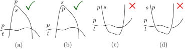
Figure 3: Bisectors intersecting twice; legal ($\checkmark$) and illegal($\times$).

[[8]] In an admissible bisector system, no cycle in the arrangment of bisectors related to $p$ can have the label $p$ on the exterior of the cycle, for all of its arcs.

Any component $\alpha$ of a bisector curve $J(p,q)$ is called an arc. We use $s_{\alpha}\in S$ to denote the site such that arc $\alpha\subseteq J(p,s_{\alpha})$. Any component of $\Gamma$ is called a $\Gamma$-arc. The arrangement of a bisector set $\mathcal{J}_{x}\subseteq\mathcal{J}$ is denoted by $\mathcal{A}(\mathcal{J}_{x})$.

3 Defining abstract Voronoi-like graphs and cycles

In order to define Voronoi-like graphs in a broader sense, we can relax axioms A1-A4 in this section. In particular, we drop axiom A1 to allow disconnected Voronoi regions and relax axiom A3 to allow disconnected (or even closed) bisecting curves. The bisector $J(p,q)$ of two sites $p,q\in S$ still subdivides the plane into two open domains: the dominance region of $p$, $D(p,q)$, and the dominance region of $q$, $D(q,p)$, however, $D(p,q)$ may be disconnected or bounded. Axioms A2 and A4 remain. Unless otherwise specified, we use the general term abstract bisector system to denote such a relaxed variant in the subsequent definitions and in Theorem 3.4. The term admissible bisector system always implies axioms A1-A4.

Let $G=(V,E)$ be a graph on the arrangement of an abstract bisector system $\mathcal{J}$, truncated within a simply connected domain $D\subseteq D_{\Gamma}$ (the leaves of $G$ are on $\partial D$). The vertices of $G$ are arrangement vertices and the edges are maximal bisector arcs connecting pairs of vertices. Figure 5 illustrates examples of such graphs on a bisector arrangment (shown in grey). Under the general position assumption, the vertices of $G$, except the leaves on $\partial D$, are of degree 3.

Definition 3.1.

A vertex $v$ in graph $G$ is called locally Voronoi, if $v$ and its incident graph edges, within a small neighborhood around $v$, $N(v)$, appear in the Voronoi diagram of the set of three sites defining $v$, denoted $S_{v}$, see Figure 4(a).

If instead we consider the farthest Voronoi diagram of $S_{v}$, then $v$ is called locally Voronoi of the farthest-type, see Figure 4(b). An ordinary locally Voronoi vertex is of the nearest-type.

Figure 4: (a) Vertex $v$ is locally Voronoi: $G\cap N(v)=\mathcal{V}(\{p,s,t\})\cap N(v)$; $N(v)$ is shaded, $G$ is bold, and bisectors are grey. (b) Vertex $v$ is locally farthest Voronoi.

Definition 3.2.

A graph $G$ on the arrangement of an abstract bisector system, enclosed within a simply connected domain $D$, is called Voronoi-like, if its vertices (other than its leaves on $\partial D$) are locally Voronoi vertices. If $G$ is disconnected, we further require that consecutive leaves on $\partial D$ have consistent labels, i.e., they are incident to the dominance region of the same site, as implied by the incident bisector edges in $G$, see Figure 5.

Figure 5: Voronoi-like graphs shown in bold on an arrangement of bisectors shown in grey.

The graph $G$ is actually called an abstract Voronoi-like graph but, for brevity, we typically skip the term abstract. We next consider the relation between a Voronoi-like graph $G$ and the Voronoi diagram $\mathcal{V}(S)\cap D$, where $S$ is the set of sites involved in the edges of $G$. Since the vertices of $G$ are locally Voronoi, each face $f$ in $G$ must have the label of exactly one site $s_{f}$ in its interior, which is called the site of $f$.

Definition 3.3.

Imagine we superimpose $G$ and $\mathcal{V}(S)\cap D$. A face $f$ of $\mathcal{V}(S)\cap D$ is said to be missing from $G$, if $f$ is covered by faces of $G$ that belong to sites that are different from the site of $f$, see Figure 7, which is derived from Figure 6.

Figure 6: A Voronoi diagram of 4 segments.

Figure 7: (a) Voronoi diagram $V(S)\cap D$; (b) Voronoi-like graph $G$; $r^{\prime}\subseteq r$; $f$ is missing from (b).

Theorem 3.4.

Let $r$ be a face of an abstract Voronoi-like graph $G$ and let $s_{r}$ denote its site (the bisectors bounding $r$ have the label $s_{r}$ inside $r$). Then one of the following holds:

1. there is a Voronoi face $r^{\prime}$ in $\mathcal{V}(S)\cap D$, of the same site $s_{r}$, $r^{\prime}\subseteq\mbox{VR}(s_{r},S)$, such that $r^{\prime}\subseteq r$, see Figure 7.

2. face $r$ is disjoint from the Voronoi region $\mbox{VR}(s_{r},S)$. Further, it is entirely covered by Voronoi faces of $\mathcal{V}(S)\cap D$, which are missing from $G$, see Figure 8.

Proof 3.5.

Imagine we superimpose $G$ and $\mathcal{V}(S)\cap D$. Face $r$ in $G$ cannot partially overlap any face of the Voronoi region $\mbox{VR}(s_{r},S)$ because if it did, some $s_{r}$-related bisector, which contributes to the boundary of $r$, would intersect the interior of $\mbox{VR}(s_{r},S)$, which is not possible by the definition of a Voronoi region. For the same reason, $r$ cannot be contained in $\mbox{VR}(s_{r},S)$. Since Voronoi regions cover the plane, the claim, except from the last sentence in item 2, follows.

Consider a Voronoi face $c^{\prime}$ of $\mathcal{V}(S)\cap D$ that overlaps with face $r$ of $G$ in case 2, where the site of $c^{\prime}$, $s_{c}$, is different from $s_{r}$. Since $c^{\prime}$ overlaps with $r$, it follows that $c^{\prime}$ cannot be entirely contained in any face of site $s_{c}$ in $G$. Furthermore, $c^{\prime}$ cannot overlap partially with any face of $s_{c}$ in $G$, by the proof in the previous paragraph. Thus, $c^{\prime}$ is disjoint from any face of $G$ of site $s_{c}$, i.e., it must be missing from $G$. In Figure 8, face $c^{\prime}$ contains $r$.

Figure 8: (a) Voronoi-like graph $G$; (b) $V(S)\cap D$; face $c^{\prime}$, which covers $r$, is missing from $G$.

Corollary 3.6.

If no Voronoi face of $\mathcal{V}(S)\cap D$ is missing from $G$, then $G=\mathcal{V}(S)\cap D$.

Let us now consider an admissible bisector system, satisfying axioms A1-A4.

Corollary 3.7.

In an admissible bisector system $\mathcal{J}$, if $D$ corresponds to the entire plane, then any Voronoi-like graph on $\mathcal{J}$ equals the Voronoi diagram of the relevant set of sites.

In an admissible bisector system, Voronoi regions are connected, thus, only faces incident to $\partial D$ may be missing from $\mathcal{V}(S)\cap D$.

Corollary 3.8.

In an admissible bisector system, any face $f$ of $G$ that does not touch $\partial D$ either coincides with or contains the Voronoi region $\mbox{VR}(s_{f},S)$.

By Corollary 3.8, in an admissible bisector system, we need to characterize the faces of a Voronoi-like graph that interact with the boundary of the domain $D$. That is, we are interested in Voronoi-like trees and forests.

Let $p$ be a site in $S$ and let $\mathcal{J}_{p}$ denote the set of $p$-related bisectors in $\mathcal{J}$.

Definition 3.9.

Let $C$ be a cycle in the arrangement of $p$-related bisectors $\mathcal{A}(\mathcal{J}_{p}\cup\Gamma)$ such that the label $p$ appears in the interior of $C$. A vertex $v$ in $C$ is called degree-2 locally Voronoi, if its two incident bisector arcs correspond to edges in the Voronoi diagram $\mathcal{V}(S_{v})$ of the three sites that define $v$ ($p\in S_{v}$). In particular, $C\cap N(v)\subseteq\mathcal{V}(S_{v})\cap N(v)$, where $N(v)$ is a small neighborhood around $v$. The cycle $C$ is called Voronoi-like, if its vertices are either degree-2 locally Voronoi or points on $\Gamma$. For brevity, $C$ is also called a $p$-cycle or site-cycle, if the site $p$ is not specified. If $C$ bounds a Voronoi region, then it is called a Voronoi cycle.

$C$ is called bounded if it contains no $\Gamma$-arcs, otherwise, it is called unbounded.

The part of the plane enclosed by $C$ is called the domain of $C$, denoted as $D_{C}$. Any $\Gamma$-arc of $C$ indicates an opening of the domain to infinity. Figure 9 illustrates a Voronoi-like cycle for site $p$, which is unbounded (see the $\Gamma$-arc $\gamma$). It is easy to see in this figure that other $p$-cycles exist, on the same set of sites, which may enclose or be enclosed by $C$. The innermost such cycle is the boundary of a Voronoi region, see Figure 10.

Figure 9: A Voronoi-like cycle for site $p$. $S_{c}=\{s,t,k,q,r,l\}$.

Let $S_{C}\subseteq S\setminus\{p\}$ denote the set of sites that (together with $p$) contribute the bisector arcs of $C$, $S_{C}=\{s_{\alpha}\in S\setminus\{p\}\mid\alpha\in C\setminus\Gamma\}$. We refer to $S_{C}$ as the set of sites relevant to $C$. Let $\hat{C}$ denote the Voronoi cycle $\hat{C}=\partial(\mbox{VR}(p,S_{C}\cup\{p\})\cap D_{\Gamma})$.

In an admissible bisector system, there can be many different Voronoi-like cycles involving the same set of sites. Any such cycle $C$ must enclose the Voronoi cycle $\hat{C}$. Further, $S_{\hat{C}}\subseteq S_{C}$. In the special case of a line arrangement, e.g., bisectors of point-sites in the Euclidean plane, a site-cycle $C$ is unique for $S_{C}$; in particular, $C=\hat{C}$.

A Voronoi-like cycle $C$ must share several bisector arcs with its Voronoi cycle $\hat{C}$, at least one bisector arc for each site in $S_{\hat{C}}$. Let $C\cap\hat{C}$ denote the sequence of common arcs between $C$ and $\hat{C}$. Several other $p$-cycles $C^{\prime}$, where $S_{\hat{C}}\subseteq S_{C^{\prime}}\subseteq S_{C}$, may lie between $C$ and $\hat{C}$, all sharing $C\cap\hat{C}$. Other $p$-cycles may enclose $C$. Figure 10 shows such cycles, where the innermost one is $\hat{C}$; its domain (a Voronoi region) is shown in solid grey.

Figure 10: Voronoi-like cycles for site $p$, $S_{c}=\{s,t,k,q,r,l\}$.

4 The Voronoi-like graph of a cycle

Let $\mathcal{J}$ be an admissible bisector system and let $C$ be a Voronoi-like cycle for site $p$, which involves a set of sites $S_{C}$ ($p\not\in S_{C}$). Let $\mathcal{J}_{C}\subseteq\mathcal{J}$ be the subset of all bisectors that are related to the sites in $S_{c}$. The cycle $C$ corresponds to a sequence of site-occurrences from $S_{C}$, which imply a Voronoi-like graph $\mathcal{V}_{l}(C)$ in the domain of $C$, defined as follows:

Definition 4.1.

The Voronoi-like graph $\mathcal{V}_{l}(C)$, implied by a Voronoi-like cycle $C$, is a graph on the underlying arrangement of bisectors $\mathcal{A}(\mathcal{J}_{C})\cap D_{C}$, whose leaves are the vertices of $C$, and its remaining (non-leaf) vertices are locally Voronoi vertices, see Figure 11.

(The existence of such a graph on $\mathcal{A}(\mathcal{J}_{C})\cap D_{C}$ remains to be established).

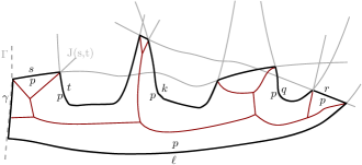
Figure 11: The Voronoi-like graph $\mathcal{V}_{l}(C)$ (red tree) of the site-cycle $C$ of Fig. 9

In this section we prove the following theorem for any Voronoi-like cycle $C$ on $\mathcal{A}(\mathcal{J}_{p}\cup\Gamma)$.

Theorem 4.2.

The Voronoi-like graph $\mathcal{V}_{l}(C)$ of a $p$-cycle $C$ has the following properties:

1. it exists and is unique;

2. it is a tree if $C$ is bounded, and a forest if $C$ is unbounded;

3. it can be computed in expected linear time, if it is the boundary of a Voronoi region. Otherwise, in expected linear time we can compute $\mathcal{V}_{l}(C^{\prime})$ for some $p$-cycle $C^{\prime}$ that is enclosed by $C$ (possibly, $C^{\prime}=C$ or $C^{\prime}=\hat{C}$).

Recall that $\hat{C}$ denotes the Voronoi-cycle enclosed by $C$, where $\hat{C}=\partial[\mbox{VR}(p,S_{C}\cup\{p\})\cap D_{\Gamma}]$. Then $\mathcal{V}_{l}(\hat{C})$ is the Voronoi diagram $\mathcal{V}(S_{C})\cap D_{\hat{C}}$. To derive Theorem 4.2 we show each item separately in subsequent lemmas.

Lemma 4.3.

Assuming that it exists, $\mathcal{V}_{l}(C)$ is a forest, and if $C$ is bounded, then $\mathcal{V}_{l}(C)$ is a tree. Each face of $\mathcal{V}_{l}(C)$ is incident to exactly one bisector arc $\alpha$ of $C$, which is called the face (or region) of $\alpha$, denoted $R(\alpha,C)$.

Proof 4.4.

We first show that $\mathcal{V}_{l}(C)$ contains no cycles. By Observation 3, any Voronoi-like cycle for a site $s\in S_{C}$ must entirely enclose $\mbox{VR}(s,S_{C})$, thus, it must also enclose $\mbox{VR}(s,S_{C}\cup\{p\})\subseteq\mbox{VR}(s,S_{C})$. Since $J(p,s)$ contributes arc(s) to $C$, it follows that $\mbox{VR}(s,S_{C}\cup\{p\})$ must extend outside of $C$, hense, $\mbox{VR}(s,S_{C})$ must also extend outside of $C$. Since $\mbox{VR}(s,S_{C})$ cannot be enclosed by $C$, the same must hold for any $s$-cycle on $S_{C}$. Thus, $\mathcal{V}_{l}(C)$ may not contain a cycle. The same argument implies that $\mathcal{V}_{l}(C)$ cannot have a face that is incident to $\Gamma$ without also being incident to a bisector arc of $C$.

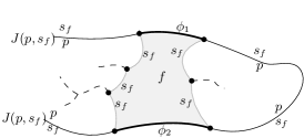
Figure 12: Proof of Lemma 4.3; face $f$ is shown shaded.

Suppose now that $\mathcal{V}_{l}(C)$ has a face $f$, which belongs to a site $s_{f}\in S_{c}$, incident to two bisector arcs $\phi_{1},\phi_{2}\in C$ such that $\phi_{1},\phi_{2}\subseteq J(p,s_{f})$, see Figure 12. Then one brunch of $\partial f\setminus\{\phi_{1},\phi_{2}\}$ and the component of $J(p,s_{f})$ between $\phi_{1}$ and $\phi_{2}$ would form a cycle having the label $s_{f}$ outside, see Figure 12. Such a cycle is not possible in an admissible bisector system, by Observation 3, deriving a contradiction. Thus, each face of $\mathcal{V}_{l}(C)$ must be incident to exactly one bisector arc.

If $C$ is the boundary of a Voronoi region, the tree property of the Voronoi diagram $\mathcal{V}(S)\cap D_{C}$ had been previously shown in [8, 4]. Lemma 4.3 generalizes it to Voronoi-like graphs for any Voronoi-like cycle $C$.

In [8], a Voronoi-like diagram was defined as a tree structure subdividing the domain of a so-called boundary curve, which was implied by a set of Voronoi edges. A boundary curve is a Voronoi-like cycle but not necessarily vice versa. That is, the tree structure of [8] was defined using some of the properties in Lemma 4.3 as definition, and the question whether such a tree always existed had remained open. In this paper a Voronoi-like graph is defined entirely differently, but Lemma 4.3 implies that the two structures are equivalent within the domain of a boundary curve. As a result, we can use and extend the results of [8].

Given a $p$-cycle $C$, and a bisector $J(p,s)$ that intersects it, an arc-insertion operation can be defined [8] as follows. Let $\alpha\subseteq J(p,s)$ be a maximal component of $J(p,s)$ in the domain of $C$, see Figure 13. Let $C_{\alpha}=C\oplus\alpha$ denote the $p$-cycle obtained by substituting with $\alpha$ the superflous portion of $C$ between the endpoints of $\alpha$. (Note that only one portion of $C$ forms a $p$-cycle with $\alpha$, thus, no ambiguity exists). There are three different main cases possible as a result, see Figure 13: 1) $\alpha$ may lie between two consecutive arcs of $C$, in which case $|C_{\alpha}|=|C|+1$; 2) $\alpha$ may cause the deletion of one or more arcs in $C$, thus, $|C_{\alpha}|\leq|C|$; 3) the endpoints of $\alpha$ may lie on the same arc $\omega$ of $C$, in which case $\omega$ splits in two different arcs, thus, $|C_{\alpha}|=|C|+2$. In all cases $C_{\alpha}$ is enclosed by $C$ ($|\cdot|$ denotes cardinality).

Figure 13: Three cases of the arc insertion operation.

The arc-insertion operation can be naturally extended to the Voronoi-like graph $\mathcal{V}_{l}(C)$ to insert arc $\alpha$ and obtain $\mathcal{V}_{l}(C_{\alpha})$. We use the following lemma, which can be extracted from [8] (using Theorem 18, Theorem 20, and Lemma 21 of [8]).

Lemma 4.5 ([8]).

Given $\mathcal{V}_{l}(C)$, arc $\alpha\in J(p,s)\cap D_{C}$, and the endpoints of $\alpha$ on $C$, we can compute the merge curve $J(\alpha)=\partial R(\alpha,C_{\alpha})$, using standard techniques as in ordinary Voronoi diagrams. If the endpoints of $\alpha$ lie on different arcs of $C$, or $\Gamma$, the time complexity is $O(|J(\alpha)|+|C\setminus C_{\alpha}|)$. Otherwise, $\alpha$ splits a bisector arc $\omega$, and its region $R(\omega,C)$, into $R(\omega_{1},C_{\alpha})$ and $R(\omega_{2},C_{\alpha})$; the time complexity increases to $O(|J(\alpha)|+\min\{|R(\omega_{1},C_{\alpha})|,|R(\omega_{2},C_{\alpha})|\})$.

The correctness proofs from [8, 10], which are related to Lemma 4.5, remain intact if performed on a Voronoi-like cycle, as long as the arc $\alpha$ is contained in the cycle’s domain; see also [10, Lemma 9]. Thus, Lemma 4.5 can be established.

Next we prove the existence of $\mathcal{V}_{l}(C)$ by construction. To this goal we use a split relation between bisectors in $\mathcal{J}_{p}$ or sites in $S_{C}$, which had also been considered in [9], see Figure 14.

Definition 4.6.

For any two sites $s,t\in S_{C}$, we say that $J(p,s)$ splits $J(p,t)$ (we also say that $s$ splits $t$, with respect to $p$), if $J(p,t)\cap D(p,s)$ contains two connected components.

Figure 14: $J(p,s)$ splits $J(p,t)$. In the partial order, $s<_{p}t$.

From the fact that related bisectors in an admissible bisector system intersect at most twice, as shown in Figs. 2 and 3, we can infer that the split relation is asymmetric and transitive, thus, it is also acyclic. The split relation induces a strict partial order on $S_{C}$, where $s<_{p}t$, if $J(p,s)$ splits $J(p,t)$, see Figure 14. Let $o_{p}$ be a topological order of the resulting directed acyclic graph, which underlies the split relation on $S_{c}$ induced by $p$.

The following lemma shows that $\mathcal{V}_{l}(C)$ exists by construction. It builds upon a more restricted version regarding a boundary curve that had been considered in [9].

Lemma 4.7.

Given the topological ordering of the split relation $o_{p}$, $\mathcal{V}_{l}(C)$ can be constructed in $O(|C|^{2})$ time; thus, $\mathcal{V}_{l}(C)$ exists. Further, at the same time, we can construct $\mathcal{V}_{l}(C^{\prime})$ for any other Voronoi-like cycle $C^{\prime}$ that is enclosed by $C$, $S_{C^{\prime}}\subseteq S_{C}$.

Proof 4.8.

Given the order $o_{p}$, we follow the randomized approach of Chew [5], and apply the arc-insertion operation of Lemma 4.5, which is extracted from [8]. Let the sites in $S_{C}$ be numbered according to $o_{p}=(s_{1},s_{2}\ldots s_{m})$, $m=|S_{C}|$. We first show that $C$ can be constructed incrementally, by arc-insertion, following $o_{p}$.

Let $C_{i}$ denote the $p$-cycle constructed by the first $i$ sites in $o_{p}$. $C_{1}$ consists of $J(s_{1},p)$ and a $\Gamma$-arc, that is, $C_{1}=\partial(D(p,s_{i})\cap D_{\Gamma})$. Clearly $C_{1}$ encloses $C$. Suppose that $C_{i}$ encloses $C$. Then, given $C_{i}$, let $C_{i+1}$ by the $p$-cycle obtained by inserting to $C_{i}$ the components of $J(s_{i+1},p)\cap D_{C_{i}}$, which correspond to arcs in $C$. For each such component $\alpha$ ($\alpha\in J(s_{i+1},p)\cap D_{C_{i}}$), if some portion of $\alpha$ appears in $C$, then compute $C_{i}\oplus\alpha$; if $\alpha$ does not appear in $C$, ignore it. Let $C_{i+1}$ be the resulting $p$-cycle after all such components of $J(s_{i+1},p)$ have been inserted to $C_{i}$, one by one. Because any site whose $p$-bisector splits $J(p,s_{i+1})$ has already been processed, a distinct component of $J(s_{i+1},p)\cap D_{C_{i}}$ must exist for each arc of $s_{i+1}$ in $C$. Thus, $C_{i+1}$ can be derived from $C_{i}$ and must enclose $C$.

We have shown that $C$ can be constructed incrementally, if we follow $o_{p}$, in time $O(|C|^{2})$. It remains to construct the Voronoi-like graph $\mathcal{V}_{l}(C_{i})$ at each step $i$. To this end, we use Lemma 4.5, starting at $\mathcal{V}_{l}(C_{1})=\emptyset$. Given $\mathcal{V}_{l}(C_{i})$ and $C_{i+1}$, we can apply Lemma 4.5 to each arc $\alpha\subseteq J(s_{i+1},p)$ in $C_{i+1}\setminus C_{i}$. The correctness proof of [8] ensures the feasibility and the correctness of each arc insertion, thus, it also ensures the existence of $\mathcal{V}_{l}(C_{i+1})$.

The above incremental construction can also compute $\mathcal{V}_{l}(C^{\prime})$ by computing both $C_{i}$ and $C_{i}^{\prime}$ at each step $i$. Suppose $C_{i}=C_{i}^{\prime}$, where $C_{1}^{\prime}=C_{1}$. When considering site $s_{i+1}$, we insert to $C_{i}^{\prime}$ all components of $J(s_{i+1},p)\cap D_{C_{i}}$ corresponding to arcs of $s_{i+1}$, which appear in either $C$ or $C^{\prime}$. Thus, $C_{i+1}^{\prime}$ is derived from $C_{i+1}$ by inserting any additional arcs $\alpha^{\prime}$ of $s_{i+1}$, where $\alpha^{\prime}\in C^{\prime}\setminus C$. Note that all arcs of $s_{i+1}$ that appear in $C$ are inserted to $C_{i+1}^{\prime}$, even if they do not appear in $C^{\prime}$. This is possible because of the order $o_{p}$: any site whose $p$-bisector splits $J(p,s_{i+1})$ has already been processed, thus, a distinct component of $J(s_{i+1},p)\cap D_{C_{i}}$ must exist for each arc of $s_{i+1}$ in either $C$ or $C^{\prime}$, which can be identified.

Referring to $\mathcal{V}_{l}(C_{i+1})$, the insertion of an additional arc $\alpha^{\prime}$ may only cause an existing region to shrink. Therefore, we derive two invariants: 1. $R(\beta,C_{i+1}^{\prime})\subseteq R(\beta,C_{i+1})$ for any arc $\beta\in C_{i+1}\cap C_{i+1}^{\prime}$; and 2. $C_{i+1}^{\prime}$ is enclosed by $C_{i}$. The invariants are maintained in subsequent steps. The fact that step $i+1$ starts with $C_{i+1}^{\prime}$, which is enclosed by $C_{i+1}$, does not make a difference to the above arguments. Thus, the invariants hold for $C_{n}$ and $C_{n}^{\prime}$, therefore, $C_{n}^{\prime}=C^{\prime}$.

The following lemma can also be extracted from [8, 10]. It can be used to establish the uniqueness of $\mathcal{V}_{l}(C)$. Similarly to Lemma 4.5, its original statement does not refer to a $p$-cycle, however, nothing in its proof prevents its adaptation to a $p$-cycle, see [10, Lemma 29].

Lemma 4.9.

[10] Let $C$ be a $p$-cycle and let $\alpha,\beta$ be two bisector arcs in $C$, where $s_{\alpha}\neq s_{\beta}$. Suppose that a component $e$ of $J(s_{\alpha},s_{\beta})$ intersects $R(\alpha,C)$. Then $J(p,s_{\beta})$ must intersect $D_{c}$ with a component $\beta^{\prime}\subseteq J(p,s_{\beta})\cap D_{c}$ such that $e$ is a portion of $\partial R(\beta^{\prime},C\oplus\beta^{\prime})$.

By Lemma 4.9, if $J(s_{\alpha},s_{\beta})$ intersects $R(\alpha,C)$, then a face of $s_{\beta}$ must be missing from $\mathcal{V}_{l}(C)$ (compared to $\mathcal{V}_{l}(\hat{C})$) implying that an arc of $J(p,s_{\beta})$ is missing from $C$. Then $\mathcal{V}_{l}(C)$ must be unique.

We now use the randomized incremental construction of [8] to construct $\mathcal{V}_{l}(C)$, which in turn follows Chew [5], to establish the last claim of Theorem 4.2. Let $o=(\alpha_{1},\ldots\alpha_{n})$ be a random permutation of the bisector arcs of $C$, where each arc represents a different occurrence of a site in $S_{C}$. The incremental algorithm works in two phases. In phase 1, delete arcs from $C$ in the reverse order $o^{-1}$, while registering their neighbors at the time of deletion. In phase 2, insert the arcs one by one, following $o$, using their neighbors information from phase 1.

Let $C_{i}$ denote the $p$-cycle constructed by considering the first $i$ arcs in $o$ in this order. $C_{1}$ is the $p$-cycle consisting of $J(s_{\alpha_{1}},p)$ and the relevant $\Gamma$-arc. Given $C_{i}$, let $\alpha_{i+1}^{\prime}$ denote the bisector component of $J(p,s_{\alpha_{i+1}})\cap D_{C_{i}}$ that contains $\alpha_{i+1}$ (if any), see Figure 13 where $\alpha$ stands for $\alpha_{i+1}^{\prime}$. If $\alpha_{i+1}$ lies outside $C_{i}$, then $\alpha_{i+1}^{\prime}=\emptyset$ (this is possible if $C_{i}$ is not a Voronoi cycle). Let cycle $C_{i+1}=C_{i}\oplus\alpha_{i+1}^{\prime}$ (if $\alpha_{i+1}^{\prime}=\emptyset$, then $C_{i+1}=C_{i}$). Given $\alpha_{i+1}^{\prime}$, and $\mathcal{V}_{l}(C_{i})$, the graph $\mathcal{V}_{l}(C_{i+1})$ is obtained by applying Lemma 4.5.

Let us point out a critical case, which differentiates from [5]: both endpoints of $\alpha_{i+1}^{\prime}$ lie on the same arc $\omega$ of $C_{i}$, see Figure 13(c) where $\alpha$ stands for $\alpha_{i+1}^{\prime}$. That is, the insertion of $\alpha_{i+1}$ splits the arc $\omega$ in two arcs, $\omega_{1}$ and $\omega_{2}$. (Note $s_{\alpha_{i+1}}<_{p}s_{\omega}$ but $\omega$ was inserted to $C_{i}$ before $\alpha_{i+1}$). Because of this split, $C_{i}$, and thus $\mathcal{V}_{l}(C_{i})$, is order-dependent: if $\alpha_{i+1}$ were considered before $\omega$, in some alternative ordering, then $\omega_{1}$ or $\omega_{2}$ would not exist in the resulting cycle, and similarly for their faces in $\mathcal{V}_{l}(C_{i+1})$. The time to split $R(\omega,C_{i})$ is proportional to the minimum complexity of $R(\omega_{1},C_{i+1})$ and $R(\omega_{2},C_{i+1})$, which is added to the time complexity of step $i$. Another side effect of the split relation is that $\alpha_{i+1}$ may fall outside $C_{i}$, if $C$ is not a Voronoi-cycle, in which case, $C_{i+1}=C_{i}$. Then $C_{n}\neq C$, in particular, $C_{n}$ is enclosed by $C$.

Because the computed cycles are order-dependent, standard backwards analysis cannot be directly applied to step $i$. In [10] an alternative technique was proposed, which can be applied to the above construction. The main difference from [10] is case $C_{i+1}=C_{i}$, however, such a case has no effect to time complexity, thus, the analysis of [10] can be applied.

Proposition 4.10.

By the variant of backwards analysis in [10], the time complexity of step $i$ is expected $O(1)$.

4.1 The relation among the Voronoi-like graphs $\mathcal{V}_{l}(C)$, $\mathcal{V}_{l}(C^{\prime})$, and $\mathcal{V}_{l}(\hat{C})$

In the following proposition, the first claim follows from Theorem 3.4 and the second follows from the proof of Lemma 4.7.

Proposition 4.11.

Let $C^{\prime}$ be a Voronoi-like cycle between $C$ and $\hat{C}$ such that $S_{\hat{C}}\subseteq S_{C^{\prime}}\subseteq S_{C}$.

1. $R(\alpha,C^{\prime})\supseteq R(\alpha,\hat{C})$, for any arc $\alpha\in C^{\prime}\cap\hat{C}$.

2. $R(\alpha,C^{\prime})\subseteq R(\alpha,C)$, for any arc $\alpha\in C\cap C^{\prime}$.

Proposition 4.11 indicates that the faces of $\mathcal{V}_{l}(C^{\prime})$ shrink as we move from the outer cycle $C$ to an inner one, until we reach the Voronoi faces of $\mathcal{V}_{l}(\hat{C})$, which are contained in all others. It also indicates that $\mathcal{V}_{l}(C)$, $\mathcal{V}_{l}(C^{\prime})$ and $\mathcal{V}_{l}(\hat{C})$ share common subgraphs, and that the adjacencies of the Voronoi diagram $\mathcal{V}_{l}(\hat{C})$ are preserved. More formally,

Definition 4.12.

Let $\mathcal{V}_{l}(C^{\prime},C\cap C^{\prime})$ be the following subgraph of $\mathcal{V}_{l}(C^{\prime})$: vertex $v\in\mathcal{V}_{l}(C^{\prime})$ is included in $\mathcal{V}_{l}(C^{\prime},C\cap C^{\prime})$, if all three faces incident to $v$ belong to arcs in $C\cap C^{\prime}$; edge $e\in\mathcal{V}_{l}(C^{\prime})$ is included to $\mathcal{V}_{l}(C^{\prime},C\cap C^{\prime})$ if both faces incident to $e$ belong to arcs in $C\cap C^{\prime}$.

Proposition 4.13.

For any Voronoi-like cycle $C^{\prime}$, enclosed by $C$, where $S_{C^{\prime}}\subseteq S_{C}$, it holds: $\mathcal{V}_{l}(C^{\prime},C\cap C^{\prime})\subseteq\mathcal{V}_{l}(C)$.

Depending on the problem at hand, computing $\mathcal{V}_{l}(C^{\prime})$ (instead of the more expensive task of computing $\mathcal{V}_{l}(C)$) may be sufficient. For an example see Section 5.

Computing $\mathcal{V}_{l}(C)$ in linear expected time, instead of $\mathcal{V}_{l}(C^{\prime})$, is possible if the faces of $\mathcal{V}_{l}(C)$ are Voronoi regions. This can be achieved by deleting the superflous arcs in $C^{\prime}\setminus C$, created during the arc-splits, which are called auxiliary arcs. A concrete example is given in Section 6. During any step of the construction, if $R(\alpha^{\prime},C_{i})$ is a Voronoi region, but $\alpha^{\prime}\cap C=\emptyset$, we can call the site-deletion procedure of [8] to eliminate $\alpha^{\prime}$ and $R(\alpha^{\prime},C_{i})$ from $\mathcal{V}_{l}(C_{i})$. In particular,

Proposition 4.14.

Given $\mathcal{V}_{l}(C_{i})$, $1\leq i\leq n$, we can delete $R(\alpha,C_{i})$, if $R(\alpha,C_{i})\subseteq\mbox{VR}(s_{\alpha},S_{\alpha})$, where $S_{\alpha}\subseteq S_{C}$ is the set of sites that define $\partial R(\alpha,C_{i})$, in expected time linear on $|S_{\alpha}|$.

There are two ways to use Proposition 4.14, if applicable:

1. Use it when necessary to maintain the invariant that $C_{i}$ encloses $C$ (by deleting [8] any auxiliary arc in $C_{i-1}$ that blocks the insertion of $\alpha_{i}$, thus, eliminating the case $C_{i}=C_{i-1}$).

2. Eliminate any auxiliary arc at the time of its creation. If the insertion of $\alpha_{i}$ splits an arc $\omega\in C_{i-1}$ into $\omega_{1}$ and $\omega_{2}$, but $\omega_{2}\not\in C$, then eliminate $R(\omega_{2},C_{i})$ by calling [8].

The advantage of the latter is that Voronoi-like cycles become order-independent, therefore, backwards analysis becomes possible to establish the algorithm’s time complexity. We give the backwards analysis argument on the concrete case of Section 6; the same type of argument, only more technical, can be derived for this abstract formulation as well.

5 Extending to Voronoi-like cycles of $k$ sites

Theorem 4.2 can extend to a Voronoi-like $k$-cycle, for brevity, a $k$-cycle, which involves a set $P$ of $k$ sites whose labels appear in the interior of the cycle. A $k$-cycle $C_{k}$ lies in the arrangement $\mathcal{A}(\mathcal{J}_{P}\cup\Gamma)$ and its vertices are degree-2 locally Voronoi, where $\mathcal{J}_{P}$ denotes the set of bisectors related to the sites in $P$. It implies a Voronoi-like graph $\mathcal{V}_{l}(C_{k})$, which involves the set of sites $S_{C}\subseteq S\setminus P$, which (together with the sites in $P$) define the bisector arcs of $C_{k}$. $\mathcal{V}_{l}(C_{k})$ is defined analogously to Def. 4.1, given $C_{k}$ and the set of sites $S_{C}$.

We distinguish two different types of $k$-cycles on $\mathcal{A}(\mathcal{J}_{P}\cup\Gamma)$: 1. a $k$-site Voronoi-like cycle whose vertices are all of the nearest type, e.g., the boundary of the union of $k$ neighboring Voronoi regions; and 2. an order-$k$ Voronoi-like cycle whose vertices are both of the nearest and the farthest type, e.g., the boundary of an order-$k$ Voronoi face. In either case we partition a $k$-cycle $C_{k}$ into maximal compound arcs, each induced by one site in $S_{C}$. Vertices in the interior of a compound arc are switches between sites in $P$, and the endpoints of compound arcs are switches between sites in $S_{c}$. For an order-$k$ cycle, the former vertices are of the farthest type, whereas the latter (endpoints of compound arcs) are of the nearest type. Given a compound arc $\alpha$, let $J(\alpha)$ denote the bisector curve that consists of the arc $\alpha$ extending the bisector arcs incident to its endpoints to $\Gamma$, see Figure 15. Let $P_{\alpha}\subseteq P$ be the subset of sites that (together with one site in $S_{C}$) define $\alpha$.

Figure 15: Bisector $J(\alpha)$ for a compound arc $\alpha$ in a $k$-site cycle (a) and an order-$k$ cycle (b).

Lemma 5.1.

Assuming that it exists, $\mathcal{V}_{l}(C_{k})$ is a forest, and if $C_{k}$ is bounded, then $\mathcal{V}_{l}(C_{k})$ is a tree. Each face of $\mathcal{V}_{l}(C_{k})$ is incident to exactly one compound arc $\alpha$ of $C_{k}$, which is denoted as $R(\alpha,C_{k})$.

Proof 5.2.

$\mathcal{V}_{l}(C_{k})$ may not contain cycles because $\mbox{VR}(s,S_{C}),s\in S_{C}$, cannot be enclosed by $C_{k}$, as in the proof of Lemma 4.3. For the same reason, any face of $\mathcal{V}_{l}(C_{k})$ must be incident to a bisector arc. Thus, $\mathcal{V}_{l}(C_{k})$ is a forest whose leaves are incident to the endpoints of compound arcs. It remains to show that no face of $\mathcal{V}_{l}(C_{k})$ can be incident to a pair of compound arcs of the same site $s\in S_{c}$.

Suppose, for the sake of contradiction, that a face $f$ is incident to two compound arcs $\alpha,\alpha^{\prime}\in C_{k}$ of the same site $s\in S_{C}$ ($s=s_{f}$). We first consider an order-$k$ cycle, see Figure 16. Arcs $\alpha$ and $\alpha^{\prime}$ consist of bisector pieces in $J(s,p_{i})$, $p_{i}\in P$. Any two of these $s$-related bisectors $J(s,p_{i})$, $J(s,p_{j})$ must intersect at least once, as otherwise $\mbox{VR}(s,\{s,p_{i},p_{j}\})$ would be disconnected, violating axiom A1. Furthermore, any two $J(s,p_{i})$ and $J(s,p_{r})$ contributing to the same compound arc must intersect exactly once, because if they intersected twice, they would intersect under an illegal pattern of Figure 3(d), see Figure 16(c).

Figure 16: Proof of Lemma 5.1 for an order-$k$ Voronoi-like cycle; face $f$ is shown shaded.

Consider the two branches of $\partial f\setminus\{\alpha,\alpha^{\prime}\}$, see Figure 16. Choose one such brunch, say $B_{1}$, and let $\alpha_{i}\subset J(s,p_{i})$ and $\alpha_{j}\subset J(s,p_{j})$ be the bisector arcs of $\alpha$ and $\alpha^{\prime}$ respectively incident to the endpoints of $B_{1}$. If $J(s,p_{i})$ and $J(s,p_{j})$ intersect at a point $I$ at opposite side of $B_{1}$ as $\alpha_{i}$ and $\alpha_{j}$, then we have a cycle formed by $B_{1}$ and the pieces of $J(s,p_{i})$ and $J(s,p_{j})$ incident to $I$ that has the label $s$ outside. But such a cycle cannot exist, by Observation 3. Thus, $I$ cannot exist and $J(s,p_{i})$, $J(s,p_{j})$ must intersect at a point $I^{\prime}$ on the other side of $B_{1}$.

Bisector $J(s,p_{i})$ (resp. $J(s,p_{j})$) cannot enter face $f$ because otherwise $J(s,p_{i})$ (resp. $J(s,p_{j})$) would intersect twice with another $s$-related bisector contributing to arc $\alpha$ (resp. $\alpha^{\prime})$, which is not possible as claimed above. Thus, $I^{\prime}$ cannot lie within $f$.

Consider the other brunch $B_{2}$ of $\partial f\setminus\{\alpha,\alpha^{\prime}\}$ and expand the arcs incident to its endpoints until one hits $J(s,p_{i})$ and the other hits $J(s,p_{j})$, see Figure 16(b). The bisectors constituting $B_{2}$ are $s$-related, thus, they must intersect $J(s,p_{i})$ and $J(s,p_{j})$, as otherwise the illegal pattern of Figure 2(b) would appear. Suppose now that $J(s,p_{i})$ and $J(s,p_{j})$ intersect at a point $I^{\prime}$ at the opposite side of $B_{2}$ as $f$. Then an illegal cycle with the label $s$ outside is constructed by the expanded brunch $B_{2}$ and the pieces of $J(s,p_{i})$ and $J(s,p_{j})$ incident to $I^{\prime}$, concluding that $I^{\prime}$ is not possible either, by Observation 3. We derive a contradiction as $J(s,p_{i})$ and $J(s,p_{j})$ must intersect at least once. Thus, each face of $\mathcal{V}_{l}(C_{k})$ must be incident to exactly one order-$k$ arc of $C_{k}$.

Suppose now that $C_{k}$ is a $k$-site Voronoi-like cycle and face $f$ is incident to compound arcs $\alpha$ and $\alpha^{\prime}$. Consider the curves $J(\alpha)$ and $J(\alpha^{\prime})$, which can not intersect $B_{1}$ nor $B_{2}$ because otherwise an illegal cycle, having the label $s$ outside, would be created contradicting Observation 3. (In Figure 15(a) an illegal cycle would be created if $J(\alpha)$ turned to intersect $B_{1}$). Furthermore, $J(\alpha)$ and $J(\alpha^{\prime})$ must intersect otherwise $\mbox{VR}(s,P_{\alpha}\cup P_{\alpha^{\prime}}\cup\{s\})$ would be disconnected. But then an illegal cycle, with the label $s$ outside, would be created between the intersecting pieces of $J(\alpha)$ and $J(\alpha^{\prime})$, and $B_{1}$ or $B_{2}$, contradicting Observation 3.

Given Lemma 5.1, the remaining claims of Theorem 4.2 can be derived as in Section 4. Let $J(s_{\alpha},P)$ denote the bisector curve associated with a compound arc $\alpha$, $s_{\alpha}\in S_{C}$. For a $k$-site cycle, $J(s_{\alpha},P)=\partial\mbox{VR}(s_{\alpha},P\cup\{s_{\alpha}\})$. For an order-$k$ cycle, $J(s_{\alpha},P)=\partial\mbox{FVR}(\alpha,P\cup\{s_{\alpha}\})$, where $\mbox{FVR}(\alpha,P\cup\{s_{\alpha}\})$ denotes the face of the farthest Voronoi region of $s_{\alpha}$, which is incident to arc $\alpha$. In both cases $J(\alpha)=J(s_{\alpha},P_{\alpha})$.

The curve $J(s_{\alpha},P)$ is expensive to compute, however, we never need to entirely compute it. Instead of $J(s_{\alpha},P)$, we use $J(s_{\alpha},\tilde{P}_{\alpha})$, where $P_{\alpha}\subseteq\tilde{P}_{\alpha}\subseteq P$, and $|P_{\alpha}|\leq|\tilde{P}_{\alpha}|\leq|P_{\alpha}|+2$. $J(s_{\alpha},\tilde{P}_{\alpha})$ is readily available from $J(\alpha)$ and the two neighbors of $\alpha$ at its insertion time in the current Voronoi-like cycle. Using $J(s_{\alpha},\tilde{P}_{\alpha})$ in the place of the $p$-bisectors of Section 3 the same essentially incremental algorithm can be applied on the compound arcs of $c_{k}$. Some properties of $J(s_{\alpha},\tilde{P}_{\alpha})$ in the case of an order-$k$ cycle are given in [10].

5.1 Computing a Voronoi-like graph in an order-$k$ Voronoi face

We now review an example by Junginger and Papadopoulou [9] when $C_{k}$ is the boundary of a face $f$ of an order-$k$ Voronoi region. It is known that $\mathcal{V}_{l}(C_{k})$ can be computed in linear-expected time [10], but an even simpler technique can be derived by computing the Voronoi-like graph of an appropriately defined Voronoi-like cycle $C$ [9]. In fact, the Voronoi-like graph of any Voronoi-like cycle $C^{\prime}$, between $C$ and $\hat{C}$, turns out fully sufficient.

Let $f$ be a face of an order-$k$ Voronoi region of a set $H$ of $k$ sites. Let $S_{f}$ denote the set of sites that, together with the sites in $H$, define the boundary $\partial f$. The graph $\mathcal{V}_{l}(\partial f)$ gives the order-$(k{+}1)$ Voronoi subdivision within $f$, which is the Voronoi diagram $\mathcal{V}(S_{f})$, truncated within $f$, i.e., $\mathcal{V}(S_{f})\cap f$.

Computing the Voronoi diagram $\mathcal{V}(S_{f})\cap f=\mathcal{V}_{l}(\partial f)$ [9].

• Given $\partial f$, and any $h\in H$, compute an $h$-cycle $C$ as implied by the order of sites along the boundary of $f$. Note that $C$ encloses the Voronoi region $\mbox{VR}(h,S_{f})$, which in turn encloses $f$. $\mbox{VR}(h,S_{f})$ is not known, however, $C$ can be derived directly from $\partial f$.

• Run the randomized incremental technique of [8] on $C$ in linear expected time (see Section 4). It will compute $\mathcal{V}_{l}(C^{\prime})$ for some $h$-cycle between $C$ and $\hat{C}$.

• Truncate $\mathcal{V}_{l}(C^{\prime})\cap f$. No matter which $h$-cycle is computed, $\mathcal{V}_{l}(C^{\prime})\cap f=\mathcal{V}(S_{f})\cap f$.

The claim follows by the fact that $R(\alpha^{\prime},\hat{C})\cap f=\emptyset$, for any $\alpha^{\prime}\in\hat{C}\setminus C^{\prime}$, and $C\setminus C^{\prime}\subseteq\hat{C}\setminus C$. Thus, $\mathcal{V}_{l}(\hat{C})\cap f=\mathcal{V}_{l}(\hat{C},\hat{C}\cap C^{\prime})\cap f=\mathcal{V}_{l}(\hat{C},\hat{C}\cap C)\cap f$.

6 Updating a constraint Delaunay triangulation

We give an example of a Voronoi-like cycle $C$, which does not correspond to a Voronoi region, but we need to compute the adjacencies of the Voronoi-like graph $\mathcal{V}_{l}(C)$. The problem appears in the incremental construction of a constraint Delaunay triangulation (CDT), a well-known variant of the Delaunay triangulation, in which a given set of segments is constrained to appear in the triangulation of a point set $Q$, which includes the endpoints of the segments, see [15] and references therein.

Every edge of the CDT is either an input segment or is locally Delaunay (see Section 1). The incremental construction to compute a CDT, first constructs an ordinary Delaunay triangulation of the points in $Q$, and then inserts segment constraints, one by one, updating the triangulation after each insertion. Shewchuk and Brown [15] gave an expected linear-time algorithm to perform each update. Although the algorithm is summarized in a pseudocode, which could then be directly implemented, the algorithmic description is quite technical having to make sense of self-intersecting polygons, their triangulations, and other exceptions. We show that the problem corresponds exactly to computing (in dual sense) the Voronoi-like graph of a Voronoi-like cycle. Thus, a very simple randomized incremental construction, with occasional calls to Chew’s algorithm [5] to delete a Voronoi region of points, can be derived. Quoting from [15]: incremental segment insertion is likely to remain the most used CDT construction algorithm, so it is important to provide an understanding of its performance and how to make it run fast. We do exactly the latter in this section.

Figure 17: Point set from [15, Fig. 3]. (a) The given CDT and the segment $s$ superimposed; (b) the cavity $P$ in blue; (c) $\mathcal{V}_{l}(C)$ in red, $C=\partial\mbox{VR}(s,S\cup\{s\})$ in black; (d) the re-triangulated $P$.

When a new constraint segment $s$ is inserted in a CDT, the triangles, which get destroyed by that segment, are identified and deleted [15]. This creates two cavities that need to be re-triangulated using constrained Delaunay triangles, see Figure 17(a),(b), borrowed from [15], where one cavity is shown shaded (in light blue) and the other unshaded. The boundary of each cavity need not be a simple polygon. However, each cavity implies a Voronoi-like cycle, whose Voronoi-like graph re-triangulates the cavity, see Figure 17(c),(d).

Figure 18: The Voronoi-like cycle $C$ and $\mathcal{V}_{l}(C)$ (in red) for the example of Fig. 17.

Let $P=(p_{1},p_{2},\ldots,p_{n})$ denote one of the cavities, where $p_{1}\ldots p_{n}$ is the sequence of cavity vertices in counterclockwise order, and $p_{1},p_{n}$ are the endpoints of $s$. Let $S$ denote the corresponding set of points ($|S|\leq n$) and let $\mathcal{J}_{s}$ denote the underlying bisector system involving the segment $s$ and points in $S$. Let $C$ be the $s$-cycle in $\mathcal{A}(\mathcal{J}_{S}\cup\Gamma)$ that has one $s$-bisector arc for each vertex in $P$, in the same order as $P$, see Figure 18. Note that one point in $S$ may contibute more than one arc in $C$.

Lemma 6.1.

The $s$-cycle $C$ exists and can be derived from $P$ in linear time.

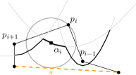
Figure 19: Proof of Lemma 6.1.

Proof 6.2.

Let $p_{i}\in P,1<i<n$. The diagonal of the original CDT, which bounded the triangle incident to $p_{i}p_{i-1}$ (resp. $p_{i}p_{i+1}$) was a locally Delaunay edge intersected by $s$. Thus, there is a circle through $p_{i}$ that is tangent to $s$ that contains neither $p_{i-1}$ nor $p_{i+1}$, see Figure 19. Hense, an arc of $J(p_{i},s)$ must exist, which contains the center of this circle, and extends from an intersection point of $J(p_{i},s)\cap J(p_{i-1},s)$ to an intersection point of $J(p_{i},s)\cap J(p_{i+1},s)$. The portion of $J(p_{i},s)$ between these two intersections corresponds to the arc of $p_{i}$ on $C$, denoted $\alpha_{i}$. Note that the $s$-bisectors are parabolas that share the same directrix (the line through $s$), thus, they may intersect twice. It is also possible that $p_{i-1}=p_{i+1}$. In each case, we can determine which intersection is relavant to arc $\alpha_{i}$, given the counterclockwise order of $P$. Such questions can be reduced to in-circle tests involving the segment $s$ and three points.

Let $\text{CDT}(P)$ denote the constraint Delaunay triangulation of $P$. Its edges are either locally Delaunay or they are cavity edges on the boundary of $P$.

Lemma 6.3.

The $\text{CDT}(P)$ is dual to $\mathcal{V}_{l}(C)$, where $C$ is the $s$-cycle derived from $P$.

Proof 6.4.

The claim derives from the definitions, Lemma 6.1, which shows the existence of $C$, and the properties of Theorem 4.2. The dual of $\mathcal{V}_{l}(C)$ has one node for each $s$-bisector arc of $C$, thus, one node per vertex in $P$. An edge of $\mathcal{V}_{l}(C)$ incident to two locally Voronoi vertices $v,u$ involves four different sites in $S$; thus, its dual edge is locally Delaunay. The dual of an edge incident to a leaf of $C$, is an edge of the boundary of $P$.

Next, we compute $\mathcal{V}_{l}(C)$ in expected linear time. Because $C$ is not the complete boundary of a Voronoi-region, if we apply the construction of Theorem 4.2, the computed cycle $C_{n}$ may be enclosed by $C$. This is because of occasional split operations, given the random order of arc-insertion, which may create auxiliary arcs that have no correspondence to vertices of $P$. However, we can use Proposition 4.14 to delete such auxiliary arcs and their faces. The sites in $S$ are points, thus, any Voronoi-like cycle in their bisector arrangement coincides with a Voronoi region. By calling Chew’s algorithm [5] we can delete any face of any auxiliary arc in expected time linear in the complexity of the face.

It is easy to dualize the technique to directly compute constraint Delaunay triangles. In fact, the cycle $C$ can remain conceptual with no need to explicitly compute it. The dual nodes are graph theoretic, each one corresponding to an $s$-bisector arc, which in turn corresponds to a cavity vertex. This explains the polygon self-crossings of [15] if we draw these graph-theoretic nodes on the cavity vertices during the intermediate steps of the construction.

The algorithm to compute $\mathcal{V}_{l}(C)$ (or its dual $\text{CDT}(C)=\text{CDT}(P)$) is very simple. Let $o=(v_{1},\ldots v_{n})$ be a random permutation of the vertices in $P$, except the endpoints of $s$; let $v_{1}=p_{1}$ and $v_{2}=p_{n}$. Let $P_{i}$ denote the sub-sequence of $P$ consisting of the first $i$ vertices in $o$. Let $C_{i}$ denote the corresponding $s$-cycle, which has one $s$-bisector arc for each vertex in $P_{i}$ in the order of $P_{i}$ (see Lemma 6.1). In an initial phase 1, starting at $P_{n}=P$, delete vertices in reverse order $o^{-1}$, recording the neighbors of each vertex $v_{i}$ in $P_{i}$ at the time of its deletion. In phase 2, consider the vertices in $o$ in increasing order, starting with $\mathcal{V}_{l}(C_{3})$, and using the arc-insertion operation (Lemma 4.5) to build $C_{i}$ and $\mathcal{V}_{l}(C_{i})$ incrementally, $3\leq i\leq n$. Instead of $\mathcal{V}_{l}(C_{i})$, we can equivalently be constructing the dual $\text{CDT}(C_{i})$.

In more detail, let $C_{3}$ be the $s$-cycle obtained by the two perpendicular lines through the endpoints of $s$, which are truncated on one side by $\Gamma$, and on the other by $J(v_{3},s)$. $C_{3}$ consists of four arcs on: $J(s,p_{1}),J(v_{3},s),J(s,p_{n})$ and $\Gamma$, respectively. $\mathcal{V}_{l}(C_{3})$ has one Voronoi vertex for $(p_{1},v_{3},p_{n})$, see Figure 21(a).

Given $\mathcal{V}_{l}(C_{i-1})$, we insert $v_{i}$ between its two neighboring vertices $w,u$, which have been recorded in phase 1. Suppose $w,v_{i},u$ appear in counterclockwise order in $P$, see Figure 20(a), where $v_{i}=v$. Let $\alpha_{i}$ denote the arc of $v_{i}$ in $C_{i}$, in particular, $\alpha_{i}$ is the component of $J(v_{i},s)\cap D_{C_{i-1}}$ whose endpoints lie between the arcs of $u$ and $w$ in $C_{i-1}$, call them $\beta$ and $\omega$ respectively, see Figure 20(a), where $\alpha_{i}=\alpha$. Among the three cases of the arc insertion operation, we only consider the split case (depicted in Figure 13(c) and 20(a)), where $J(v_{i},s)$ splits (intersects twice) the arc $\omega\subseteq J(w,s)$ in $C_{i-1}$; the other cases are straightforward. In this case, when inserting $\alpha_{i}$ to $\mathcal{V}_{l}(C_{i-1})$, the region $R(\omega,C_{i-1})$ is split in two faces, where one, say $R(\omega_{2},C_{i})$, does not correspond to $w$ (since it is out of order with respect to $w,v_{i},u$). That is, we compute $\mathcal{V}_{l}(C_{i}^{\prime})$, where $C_{i}^{\prime}=C_{i-1}\oplus\alpha_{i}$ and includes the auxiliary arc $\omega_{2}$. To obtain $\mathcal{V}_{l}(C_{i})$ we can call Chew’s algorithm to delete $R(\omega_{2},C_{i}^{\prime})$, thus, restore $C_{i}$ to its original definition. The increase to the time complexity of step $i$ is expected $O(|R(\omega_{2},C_{i})|$. This is not covered by the argument of [10], which proves the expected constant time complexity of step $i$. However, by deleting auxiliary arcs, $\mathcal{V}_{l}(C_{i})$ becomes order-independent, therefore, we can prove the time complexity of step $i$ in simpler terms by invoking backwards analysis.

Lemma 6.5.

The time complexity of step $i$, which computes $\mathcal{V}_{l}(C_{i})$ enhanced by calling Chew’s algorithm to delete any generated auxiliary arc, is expected $O(1)$.

Proof 6.6.

Since $C_{i-1}$ contains no auxiliary arcs, step $i$ can be performed in time proportional to $|R(\alpha_{i},C_{i}^{\prime})|$ + $|R(\omega_{2},C_{i}^{\prime})|$, where $C_{i}^{\prime}=C_{i-1}\oplus\alpha_{i}$, and $\omega_{2}$ is the auxiliary arc when inserting $\alpha_{i}$ to $\mathcal{V}_{l}(C_{i-1})$. The first term $|R(\alpha_{i},C_{i}^{\prime})|\leq|R(\alpha_{i},C_{i})|$. The second term can be expressed as $|R(\omega_{2},C_{i}\oplus\omega_{2}|)$, i.e, the face complexity of $\omega_{2}$, if we insert the arc $\omega_{2}$ to $\mathcal{V}_{l}(C_{i})$. We charge 1 unit, on behalf of $v_{i}$, to any vertex of $\mathcal{V}_{l}(C_{i})$ that would get deleted if we inserted the arc $\omega_{2}$.

Let $V_{i}=\{v_{3}\ldots v_{i}\}$. Any vertex in $V_{i}$ is equally likely to be the last one considered at step $i$. Thus, we can add up the time complexity of step $i$ when considering each vertex in $V_{i}$ as last, and take the average. The total is $O(|\mathcal{V}_{l}(C_{i})|)$ for the first term, plus the total number of charges for the second. By the following lemma the total number of charges is also $O(|\mathcal{V}_{l}(C_{i})|)$. Therefore, the average time complexity is $O(1)$.

Figure 20: Proof of Lemma 6.7.

Lemma 6.7.

At step $i$, any vertex of $\mathcal{V}_{l}(C_{i})$ can be charged at most twice.

Proof 6.8.

Consider a vertex $t$ of $\mathcal{V}_{l}(C_{i})$ and its Delaunay circle $C_{t}$ passing through three vertices of $P_{i}$, indicated by crosses in Figure 20(b). The three vertices partition $C_{t}$ in three arcs: $A_{1},A_{2},A_{3}$. The segment $s$ must cross through (intersect twice) one of these arcs, say $A_{1}$, since $s$ must be visible to $t$ and the three defining sites of $C_{t}$.

Suppose $t$ is charged one unit by $v\in V_{i}$. Suppose $w,v,u$ appear consecutively counterclockwise around $P_{i}$. Let $\omega,\beta$ be the arcs corresponding to $w$ and $u$, respectively, in $C_{i-1}$, see Figure 20(a). Since $t$ is charged one unit by $v$, it follows that $\omega\in C_{i-1}$ gets split by the insertion of $v$ creating an auxiliary arc $\omega_{2}$, and $t$ lies in $R(\omega_{2},C_{i}\oplus\omega_{2})$. That is, $w$ is enclosed by $C_{t}$ but $v$ and $u$ are not. Thus, diagonal $vu$ must intersect $C_{t}$, and since it cannot obstruct the visibility between $s$ and the defining points of $C_{t}$, it must cross through another arc of $C_{t}$, say $A_{2}$; diagonal $uv$ leaves $w$ and $t$ on opposite sides. But $s$ must be visible to diagonal $uv$, thus, no other diagonal of $P_{i}$ can also cross through $A_{2}$, obstructing the visibility of $uv$ and $s$. Thus, $v$ can receive at most one charge in relation to arc $A_{2}$. This implies that $v$ can receive at most one more charge in total, which corresponds to $A_{3}$.

Figure 21 illustrates the incremental construction for an indicated order $o=(v_{1},\ldots,v_{6})$. Vertices $v_{4}$ and $v_{6}$ coincide. The insertion of $v_{5}$ causes the arc of $v_{4}$ to split, see Fig. 21(c). The result of deleting the created auxiliary arc is shown in Fig. 21(d); we insert $v_{6}$ in Fig. 21(e). In this example, we could avoid deleting the auxiliary arc of $v_{4}$, which is created by inserting $v_{5}$ in Fig. 21(c), because it overlaps with an arc of $C$, therefore, it is known that it will later be re-inserted and it cannot obstruct the insertion process of other arcs.

Figure 21: The incremental construction following $o=(v_{1},\ldots,v_{6})$. (a) $\mathcal{V}_{l}(C_{3})$; (b) $\mathcal{V}_{l}(C_{4})$; (c) $\mathcal{V}_{l}(C_{5}^{\prime})$; (d) $\mathcal{V}_{l}(C_{5})$; (e) $\mathcal{V}_{l}(C_{6})$.

7 Concluding remarks

We have also considered the variant of computing, in linear expected time, a Voronoi-like tree (or forest) within a simply connected domain $D$, of constant boundary complexity, given the ordering of some Voronoi faces along the boundary of $D$. In an extended paper, we will provide conditions under which the same essentially technique can be applied.

In future research, we are also interested in considering deterministic linear-time algorithms to compute abstract Voronoi-like trees and forests as inspired by [1].

References

- [1] Alok Aggarwal, Leonidas J. Guibas, James B. Saxe, and Peter W. Shor. A linear-time algorithm for computing the Voronoi diagram of a convex polygon. Discrete and Computational Geometry, 4:591–604, 1989.
- [2] Franz Aurenhammer, Rolf Klein, and Der-Tsai Lee. Voronoi Diagrams and Delaunay Triangulations. World Scientific, 2013.
- [3] Cecilia Bohler, Rolf Klein, and Chih-Hung Liu. Abstract Voronoi diagrams from closed bisecting curves. International Journal of Computational Geometry and Applications, 2017.
- [4] Cecilia Bohler, Rolf Klein, and Chih-Hung Liu. An efficient randomized algorithm for higher-order abstract voronoi diagrams. Algorithmica, 81(6):2317–2345, 2019.
- [5] L. Paul Chew. Building Voronoi diagrams for convex polygons in linear expected time. Technical report, Dartmouth College, Hanover, USA, 1990.
- [6] B. Delaunay. Sur la sphère vide. A la memoire de Georges Voronoiï. Bulletin de l’Académie des Sciences de l’URSS, 6:793–800, 1934.
- [7] H. Edelsbrunner and R. Seidel. Voronoi diagrams and arrangements. Discrete and Comptational Geometry, 1:25–44, 1986.
- [8] Kolja Junginger and Evanthia Papadopoulou. Deletion in Abstract Voronoi Diagrams in Expected Linear Time. In 34th International Symposium on Computational Geometry (SoCG), volume 99 of LIPIcs, pages 50:1–50:14, Dagstuhl, Germany, 2018.
- [9] Kolja Junginger and Evanthia Papadopoulou. On tree-like abstract Voronoi diagrams in expected linear time. In CGWeek Young Researchers Forum (CG:YRF), 2019.
- [10] Kolja Junginger and Evanthia Papadopoulou. Deletion in abstract Voronoi diagrams in expected linear time and related problems. arXiv:1803.05372v2 [cs.CG], 2020. To appear in Discrete and Computational Geometry.
- [11] Rolf Klein. Concrete and Abstract Voronoi Diagrams, volume 400 of Lecture Notes in Computer Science. Springer-Verlag, 1989.
- [12] Rolf Klein, Elmar Langetepe, and Z. Nilforoushan. Abstract Voronoi diagrams revisited. Computational Geometry: Theory and Applications, 42(9):885–902, 2009.
- [13] Rolf Klein, Kurt Mehlhorn, and Stefan Meiser. Randomized incremental construction of abstract Voronoi diagrams. Computational Geometry: Theory and Applications, 3:157–184, 1993.
- [14] Micha Sharir and Pankaj K. Agarwal. Davenport-Schinzel sequences and their geometric applications. Cambridge university press, 1995.
- [15] Jonathan Richard Shewchuk and Brielin C. Brown. Fast segment insertion and incremental construction of constrained Delaunay triangulations. Computational Geometry: Theory and Applications, 48(8):554–574, 2015.