About the de Almeida-Thouless line in neural networks

Abstract

In this work we present a rigorous and straightforward method to detect the onset of the instability of replica-symmetric theories in information processing systems, which does not require a full replica analysis as in the method originally proposed by de Almeida and Thouless for spin glasses. The method is based on an expansion of the free-energy obtained within one-step of replica symmetry breaking (RSB) around the RS value. As such, it requires solely continuity and differentiability of the free-energy and it is robust to be applied broadly to systems with quenched disorder. We apply the method to the Hopfield model and to neural networks with multi-node Hebbian interactions, as case studies. In the appendices we test the method on the Sherrington-Kirkpatrick and the Ising $P$-spin models, recovering the AT lines known in the literature for these models, as a special limit, which corresponds to assuming that the transition from the RS to the RSB phase can be obtained by varying continuously the order parameters. Our method provides a generalization of the AT approach, which does not rely on this limit and can be applied to systems with discontinuous phase transitions, as we show explicitly for the spherical P-spin model, recovering the known RS instability line.

1 Introduction

Replica symmetry breaking in neural networks has attracted increasing attention in recent years Albanese2021 ; Zecchina-Pnas2016 ; Zecchina-PRL2021 ; Haiping-PRR2023 ; Gavin-PRE2022 , however there is, as yet, no general broken replica-symmetry theory for these systems and no simple method to systematically detect their transition from the replica-symmetric (RS) to the replica-symmetry-broken (RSB) phase.

While the first point is still out of reach, the second question can be addressed by adapting approaches originally developed for spin glasses. Indeed, the instability line of the RS phase in the Sherrington-Kirkpatrick (SK) spin glass model was derived by de Almeida and Thouless (AT) many decades ago de1978stability , using a method based on replicas. Since their seminal work, rigorous techniques have been developed and tested in archetypical mean-field as well as short-ranged spin glass models, by many researchers (see e.g. talagrand2003spin ; bardina2004 ; guerra2006replica ; chen2021almeida ; Holler-PRE2020 ; Chokri-JSP2022 ; Charbonneau-PRE2019 ; Kondor-arxiv2022 ).

As neural networks are particular realizations of spin glasses, it is quite natural to ask if we can devise a systematic method to derive the RS instability line also for these systems. In this work we answer affirmatively to this question, using the Hopfield model of neural networks and a model of dense associative memory, which extends Hebbian learning to multi-node interactions, as case studies. To this purpose, we devise a method inspired by the approach proposed by Toninelli in toninelli2002almeida , which builds on Guerra’s work on broken replica-symmetry bounds guerra_broken . As a technical note we remark that at difference with conventional spin glasses, here we focus on the RS instability in the parameter space $(\alpha,T)$ where $\alpha$ is the storage load of the network and $T$ is the noise level, rather than in the space $(h,T)$ (i.e. magnetic field, temperature) conventionally used in spin glasses.

For the Hopfield model, our method recovers the instability line obtained by Coolen coolen2001statistical using the AT approach, as a special limit, which corresponds to assuming a continuous transition from the RS to the RSB phase, in the order parameters. Therefore, our method provides a generalization of the AT approach, which can be applied to systems with a discontinuous transition from the RS to the 1RSB phase. Another advantage of our method, when compared to the involved calculations of the AT method in the Hopfield model coolen2001statistical , is its remarkable simplicity. This allows for straightforward application to more complex neural network models, such as dense associative memories with $P$-node interactions. We supplement the results in the main text with appendix A where we show our method at work on conventional spin-glass models, namely the Sherrington-Kirkpatrick model, the Ising $P$-spin and the spherical $P$-spin model, the latter providing an example of system which exhibits a discontinuous phase transition from the RS to the RSB phase. In all cases, we retrieve the AT lines known for these models de1978stability ; gardner1985spin ; Crisanti ; coolen2001statistical in a specific limit, confirming the validity of our approach as a generalization of the AT method. As expected from the decomposition theorem of multi-node Hebbian networks proved in Albanese2021 , for dense associative memories with $P$-node interactions we retrieve the instability line of the Ising $P$-spin model derived in Appendix A. Appendices B and C provide further technical details.

2 The Hopfield model

In this section we illustrate the method for the Hopfield model with $N$ Ising neurons $\sigma_{i}\in\{1,-1\},\ i=1,\ldots,N$ and $K=\alpha N$ stored patterns $\bm{\xi}^{\mu}$, $\mu=1,\ldots,K$. Each pattern $\bm{\xi}^{\mu}$ is a sequence of $N$ Rademacher entries (i.e. Bernoulli variables) $\xi_{i}^{\mu}$, $i=1,\ldots,N$, with distribution

$$\mathbb{P}(\xi_{i}^{\mu})=\dfrac{1}{2}\left(\delta_{\xi_{i}^{\mu},+1}+\delta_{\xi_{i}^{\mu},-1}\right).$$ (1)

The Hamiltonian of the model is

$$H_{N}(\bm{\sigma}|\bm{\xi})=-\dfrac{1}{N}\sum_{i,j=1,1}^{N,N}\sum_{\mu=1}^{K}\xi^{\mu}_{i}\xi^{\mu}_{j}\sigma_{i}\sigma_{j}$$ (2)

and we denote the associated Boltzmann factor, at inverse temperature $\beta=1/T$, as

$$\mathcal{B}_{N}(\bm{\sigma}|\bm{\xi})=\frac{e^{-\beta H_{N}(\bm{\sigma}|\bm{\xi})}}{Z},\quad\quad\quad Z=\sum_{{\bm{\sigma}}}e^{-\beta H_{N}(\bm{\sigma}|\bm{\xi})}.$$ (3)

In the so-called ‘retrieval’ phase, the equilibrium local configurations are correlated only with a single pattern, say $\nu$. As the couplings $J_{ij}=\sum_{\mu=1}^{K}\xi^{\mu}_{i}\xi^{\mu}_{j}$ are symmetric w.r.t. permutations of the patterns, it is assumed without loss of generality that $\nu=1$. It is then convenient to define as the order parameters of the system, the so-called Mattis magnetization

$$m({\bm{\sigma}}):=\dfrac{1}{N}\displaystyle\sum\limits_{i=1}^{N}\xi_{i}^{1}\sigma_{i}$$ (4)

which quantifies the alignment of the system configuration ${\bm{\sigma}}$ with the retrieval pattern $\bm{\xi}^{1}$, and the two-replica overlap

$$q({\bm{\sigma}}^{(1)},{\bm{\sigma}}^{(2)})\!\!:=\dfrac{1}{N}\displaystyle\sum\limits_{i=1}^{N}\sigma_{i}^{(1)}\sigma_{i}^{(2)}$$ (5)

which quantifies the correlations between two configurations ${\bm{\sigma}}^{(1)},{\bm{\sigma}}^{(2)}$ of the system, with the same realization of the patterns (i.e. quenched disorder).

The RS analysis assumes that the order parameters $m$ and $q$ self-average around their equilibrium values ${\bar{m}}$ and $\bar{q}$, in the thermodynamic limit, namely

$$\lim_{N\rightarrow+\infty}P_{N}(m)= \delta(m-\bar{m}),$$ (6)

$$\lim_{N\rightarrow+\infty}P^{\prime}_{N}(q)= \delta(q-\bar{q}),$$ (7)

where $P_{N}(m)=\mathbb{E}_{\bm{\xi}}\sum_{\bm{\sigma}}\mathcal{B}_{N}(\bm{\sigma}|\bm{\xi})\delta(m-m(\bm{\sigma}))$ and $P_{N}^{\prime}(q)=\mathbb{E}_{\bm{\xi}}\sum_{{\bm{\sigma}}^{(1)},{\bm{\sigma}}^{(2)}}\mathcal{B}_{N}(\sigma^{(1)}|\bm{\xi})\mathcal{B}_{N}({\bm{\sigma}}^{(2)}|\bm{\xi})\delta(q-q_{12}({\bm{\sigma}}^{(1)},{\bm{\sigma}}^{(2)}))$, with $\mathbb{E}_{\bm{\xi}}$ denoting the expectation over the pattern distribution (or ’quenched’ disorder). Under this assumption, the free-energy, averaged over the pattern distribution, $f$, is given by (see Amit )

$$-\beta f_{RS}({\bar{m}},\bar{q}|\beta,\alpha)= \ln 2-\dfrac{\alpha}{2}\ln(1-\beta(1-\bar{q}))-\dfrac{\beta}{2}{\bar{m}}^{2}+\dfrac{\alpha\beta\bar{q}}{2(1-\beta(1-\bar{q}))}$$

$$-\dfrac{\alpha\beta^{2}}{2}\dfrac{\bar{q}(1-\bar{q})}{(1-\beta(1-\bar{q}))^{2}}+\mathbb{E}\ln\cosh\left(\beta z\sqrt{\dfrac{\alpha\bar{q}}{(1-\beta(1-\bar{q}))^{2}}}+\beta{\bar{m}}\right),$$ (8)

where $z$ is a random Gaussian variable with zero average and unit variance, $\mathbb{E}$ denotes the average over $z$ and $\alpha$ is the load capacity of the network. In this limit, the order parameters $\bar{q}$ and ${\bar{m}}$ fulfill the celebrated Amit-Gutfreund-Sompolinsky self-consistency equations Amit ; Coolen :

$$\bar{q} =\mathbb{E}\tanh^{2}\left(\beta{\bar{m}}+\beta\sqrt{\dfrac{\alpha\bar{q}}{(1-\beta(1-\bar{q}))^{2}}}z\right),$$ (9)

$${\bar{m}} =\mathbb{E}\tanh\left(\beta{\bar{m}}+\beta\sqrt{\dfrac{\alpha\bar{q}}{(1-\beta(1-\bar{q}))^{2}}}z\right).$$ (10)

On the other hand, within one step of the replica-symmetry breaking (1RSB) scheme Crisanti-RSB ; Steffan-RSB ; AABO-JPA2020 it is assumed that the distribution of the two-replica overlap $q$, in the thermodynamic limit, displays two delta-peaks at the equilibrium values $\bar{q}_{0}$ and $\bar{q}_{1}>\bar{q}_{0}$ and the concentration on these two values is ruled by the parameter $\theta\in[0,1]$, while $m$ self-averages as in the RS case :

$${\color[rgb]{0,0,0}\lim_{N\rightarrow+\infty}P_{N}(m)} {\color[rgb]{0,0,0}=\delta(m-\bar{m}_{1})},$$ (11)

$$\lim_{N\rightarrow+\infty}P^{\prime}_{N}(q) =\theta\delta(q-\bar{q}_{0})+(1-\theta)\delta(q-\bar{q}_{1}),$$ (12)

Within this assumption, the disorder-averaged free-energy is given by (see e.g. AABO-JPA2020 )

$$-\beta f_{1RSB}({\bar{m}_{1}},\bar{q}_{1},\bar{q}_{0}|\beta,\alpha,\theta) =\ln 2-\dfrac{\alpha}{2}\ln\left(\Delta_{1}(\beta,\bar{q}_{1})\right)+\dfrac{\alpha}{2\theta}\ln\left(\dfrac{\Delta_{1}(\beta,\bar{q}_{1})}{\Delta_{2}(\beta,\theta,\bar{q}_{0},\bar{q}_{1})}\right)+\dfrac{\alpha\beta\bar{q}_{0}}{2\Delta_{2}(\beta,\theta,\bar{q}_{0},\bar{q}_{1})}$$

$$-\dfrac{\beta}{2}{\bar{m}_{1}}^{2}+\frac{1}{2}\alpha\beta^{2}\theta\frac{\bar{q}_{0}^{2}}{\Delta_{2}^{2}(\beta,\theta,\bar{q}_{0},\bar{q}_{1})}+\dfrac{1}{\theta}\mathbb{E}_{1}\ln\mathbb{E}_{2}\cosh^{\theta}g_{\theta}(\beta,\alpha,{\bar{m}_{1}},\bar{q}_{0},\bar{q}_{1})$$

$$-\frac{1}{2}\alpha\beta^{2}\theta\bar{q}_{1}\!\left(\frac{\bar{q}_{0}}{\Delta_{2}^{2}(\beta,\theta,\bar{q}_{0},\bar{q}_{1})}+\frac{\bar{q}_{1}-\bar{q}_{0}}{\Delta_{1}(\beta,\bar{q}_{1})\Delta_{2}(\beta,\theta,\bar{q}_{0},\bar{q}_{1})}\!\right)$$

$$-\frac{1}{2}\alpha\beta^{2}(1\!-\!\bar{q}_{1})\!\left(\frac{\bar{q}_{0}}{\Delta_{2}^{2}(\beta,\theta,\bar{q}_{0},\bar{q}_{1})}\!+\!\frac{\bar{q}_{1}-\bar{q}_{0}}{\Delta_{1}(\beta,\bar{q}_{1})\Delta_{2}(\beta,\theta,\bar{q}_{0},\bar{q}_{1})}\!\right)$$ (13)

where, for mathematical convenience, we defined

$$\Delta_{1}(\beta,\bar{q}_{1}):=1-\beta(1-\bar{q}_{1})$$ (14)

$$\Delta_{2}(\beta,\theta,\bar{q}_{0},\bar{q}_{1}):=1-\beta(1-\bar{q}_{1})-\beta\theta(\bar{q}_{1}-\bar{q}_{0})$$ (15)

$$g_{\theta}(\beta,\alpha,{\bar{m}_{1}},\bar{q}_{1},\bar{q}_{0}):=\beta{\bar{m}_{1}}+\frac{\beta z^{(1)}\sqrt{\alpha\bar{q}_{0}}}{\Delta_{2}(\beta,\theta,\bar{q}_{0},\bar{q}_{1})}+\beta z^{(2)}\sqrt{\frac{\alpha(\bar{q}_{1}-\bar{q}_{0})}{\Delta_{1}(\beta,\bar{q}_{1})\Delta_{2}(\beta,\theta,\bar{q}_{0},\bar{q}_{1})}}$$ (16)

and we have denoted with $\mathbb{E}_{1}$, $\mathbb{E}_{2}$ the averages w.r.t. the standard normal variables $z^{(1)}$ and $z^{(2)}$, respectively. From now on, we imply the dependence of all the functions on $\beta$ and $\alpha$. By extremizing the 1RSB free-energy w.r.t. its order parameters $\bar{q}_{0},\ \bar{q}_{1},\ {\bar{m}_{1}}$, it is possible to show that the latter fulfill the following self-consistency equations

$$\begin{array}[]{lll}{\bar{m}_{1}}&=\mathbb{E}_{1}\left[\dfrac{\mathbb{E}_{2}\cosh^{\theta}{g_{\theta}({\color[rgb]{0,0,0}{\bar{m}_{1}},\,}\bar{q}_{1},\bar{q}_{0})}\tanh{g_{\theta}({\color[rgb]{0,0,0}{\bar{m}_{1}},\,}\bar{q}_{1},\bar{q}_{0})}}{\mathbb{E}_{2}\cosh^{\theta}{g_{\theta}({\color[rgb]{0,0,0}{\bar{m}_{1}},\,}\bar{q}_{1},\bar{q}_{0})}}\right],\\ \\ \bar{q}_{1}&=\mathbb{E}_{1}\left[\dfrac{\mathbb{E}_{2}\cosh^{\theta}{g_{\theta}({\color[rgb]{0,0,0}{\bar{m}_{1}},\,}\bar{q}_{1},\bar{q}_{0})}\tanh^{2}{g_{\theta}({\color[rgb]{0,0,0}{\bar{m}_{1}},\,}\bar{q}_{1},\bar{q}_{0})}}{\mathbb{E}_{2}\cosh^{\theta}{g_{\theta}({\color[rgb]{0,0,0}{\bar{m}_{1}},\,}\bar{q}_{1},\bar{q}_{0})}}\right],\\ \\ \bar{q}_{0}&=\mathbb{E}_{1}\left[\dfrac{\mathbb{E}_{2}\cosh^{\theta}{g_{\theta}({\color[rgb]{0,0,0}{\bar{m}_{1}},\,}\bar{q}_{1},\bar{q}_{0})}\tanh{g_{\theta}({\color[rgb]{0,0,0}{\bar{m}_{1}},\,}\bar{q}_{1},\bar{q}_{0})}}{\mathbb{E}_{2}\cosh^{\theta}{g_{\theta}({\color[rgb]{0,0,0}{\bar{m}_{1}},\,}\bar{q}_{1},\bar{q}_{0})}}\right]^{2}.\end{array}$$ (17)

The key idea of our method is to assume that at the onset of the RS instability, one of the two delta-peaks in equation (12) has vanishing weight, i.e. either $\theta\!\to\!0$ or $\theta\!\to\!1$. Consistency with the RS theory then requires the dominating peak to be located at the value $\bar{q}$ of the RS order parameter, so either $\lim_{\theta\to 0}\bar{q}_{1}\!=\!\bar{q}$ or $\lim_{\theta\to 1}\bar{q}_{0}\!=\!\bar{q}$. As we will see below, both these relations are generally satisfied, hence we appeal to the physical interpretation of RS breaking to determine which scenario applies. Noting that when the RS theory becomes unstable, a multiplicity of states emerges with mutual overlap $\bar{q}_{0}$ and self-overlap $\bar{q}_{1}$, within the single state (or each of the states) predicted by the RS theory, it is natural to assume that the value of the mutual overlap between the newly born states is equal to the self-overlap $\bar{q}$ of the state(s) assumed by the RS theory. Thus, we will assume that at the onset of the RS instability, $\bar{q}_{0}\to\bar{q}$, hence $\theta\to 1$. For the Hopfield model, taking this limit in (17), and using

$$g_{1}({\color[rgb]{0,0,0}{\bar{m}_{1}},\,}\bar{q}_{1},\bar{q}_{0})=\beta{\bar{m}_{1}}+\beta z^{(1)}\dfrac{\sqrt{\alpha\bar{q}_{0}}}{\Delta_{1}(\bar{q}_{0})}+\beta z^{(2)}\sqrt{\dfrac{\alpha(\bar{q}_{1}-\bar{q}_{0})}{\Delta_{1}(\bar{q}_{1})\Delta_{1}(\bar{q}_{0})}},$$ (18)

we get

$$\lim_{\theta\to 1}\bar{q}_{0} =\mathbb{E}_{1}\left[\dfrac{\mathbb{E}_{2}\sinh{g_{1}({\color[rgb]{0,0,0}{\bar{m}_{1}},\,}\bar{q}_{1},\bar{q}_{0})}}{\mathbb{E}_{2}\cosh{g_{1}({\color[rgb]{0,0,0}{\bar{m}_{1}},\,}\bar{q}_{1},\bar{q}_{0})}}\right]^{2}$$

$$=\mathbb{E}_{1}\left[\dfrac{\exp\left(\dfrac{\beta^{2}\alpha(\bar{q}_{1}-\bar{q}_{0})}{2\Delta_{1}(\bar{q}_{1})\Delta_{1}(\bar{q}_{0})}\right)\sinh\left(\beta{\bar{m}_{1}}+\beta\sqrt{\dfrac{\alpha\bar{q}_{0}}{(1-\beta(1-\bar{q}_{0}))^{2}}}z^{(1)}\right)}{\exp\left(\dfrac{\beta^{2}\alpha(\bar{q}_{1}-\bar{q}_{0})}{2\Delta_{1}(\bar{q}_{1})\Delta_{1}(\bar{q}_{0})}\right)\cosh\left(\beta{\bar{m}_{1}}+\beta\sqrt{\dfrac{\alpha\bar{q}_{0}}{(1-\beta(1-\bar{q}_{0}))^{2}}}z^{(1)}\right)}\right]^{2}$$

$$=\mathbb{E}_{1}\tanh^{2}\left(\beta{\bar{m}_{1}}+\beta\sqrt{\dfrac{\alpha\bar{q}_{0}}{(1-\beta(1-\bar{q}_{0}))^{2}}}z^{(1)}\right)$$ (19)

where in the second line we have used $\sinh(A+B)=\sinh A\cosh B+\sinh B\cosh A$ and $\cosh(A+B)=\cosh A\cosh B+\sinh B\sinh A$ ($A$ denoting the first two terms on the RHS of (18) and $B$ the last one) and have performed the integral over $z^{(2)}$ using the oddity of the $\sinh$ function. As (19) is identical to (9), in the limit $\theta\to 1$, $\bar{q}_{0}$ is indeed equal to the RS order parameter $\bar{q}$, as anticipated. Similarly, we can show that

$$\lim_{\theta\to 1}{\bar{m}_{1}} ={\bar{m}}$$ (20)

and one can easily verify that $f_{1RSB}({\bar{m}_{1}},\bar{q}_{1},\bar{q}_{0}|\theta)|_{\theta=1}=f_{RS}({\bar{m}},\bar{q})$, as expected from the fact that, for $\theta=1$, Eq. (12) reduces to (7) and one retrieves the RS scheme. Our purpose is then to prove that for values of $\theta$ close but away from one, the 1RSB expression of the quenched free-energy is smaller than the RS expression, i.e. $f_{1RSB}({\bar{m}_{1}},\bar{q}_{1},\bar{q}_{0}|\theta)<f_{RS}({\bar{m}},\bar{q})$, below a critical line in the parameters space $(\alpha,\beta)$.

To this purpose, we expand the 1RSB quenched free-energy around $\theta=1$ (i.e. around the replica symmetric expression) to the first order, writing

$$f_{1RSB}({\color[rgb]{0,0,0}{\bar{m}_{1}},\,}\bar{q}_{1},\bar{q}_{0}|\theta)= f_{1RSB}({\color[rgb]{0,0,0}{\bar{m}_{1}},\,}\bar{q}_{1},\bar{q}_{0}|\theta)|_{\theta=1}+(\theta-1)\partial_{\theta}f_{1RSB}({\color[rgb]{0,0,0}{\bar{m}_{1}},\,}\bar{q}_{1},\bar{q}_{0}|\theta)|_{\theta=1},$$ (21)

where $f_{1RSB}({\color[rgb]{0,0,0}{\bar{m}_{1}},\,}\bar{q}_{1},\bar{q}_{0}|\theta)|_{\theta=1}=f_{RS}({\color[rgb]{0,0,0}{\bar{m}},\,}\bar{q})$. To determine when the RS solution becomes unstable, i.e. $f_{1RSB}({\color[rgb]{0,0,0}{\bar{m}_{1}},\,}\bar{q}_{1},\bar{q}_{0}|\theta)<f_{RS}({\color[rgb]{0,0,0}{\bar{m}},\,}\bar{q})$ we inspect the sign of $\partial_{\theta}f_{1RSB}({\color[rgb]{0,0,0}{\bar{m}_{1}},\,}\bar{q}_{1},\bar{q}_{0}|\theta)|_{\theta=1}$, keeping in mind that $\theta-1<0$. To evaluate the latter, we need to expand the self-consistency equations for ${\bar{m}_{1}},$ $\bar{q}_{0}$ and $\bar{q}_{1}$ around $\theta=1$, to linear orders in $\theta-1$. We obtain

$$\bar{q}_{0} =\mathbb{E}_{1}\tanh^{2}\left(\beta{\bar{m}}+\beta\sqrt{\dfrac{\alpha\bar{q}_{0}}{(1-\beta(1-\bar{q}_{0}))^{2}}}z^{(1)}\right)+(\theta-1)A({\color[rgb]{0,0,0}{\bar{m}_{1}},\,}\bar{q}_{0},\bar{q}_{1})$$ (22)

where $A({\color[rgb]{0,0,0}{\bar{m}_{1}},\,}\bar{q}_{0},\bar{q}_{1})$ is a function of ${\color[rgb]{0,0,0}{\bar{m}_{1}}}$, $\bar{q}_{0}$ and $\bar{q}_{1}$ that will drop out of the calculation, whose expression is provided in (117). As to $\mathcal{O}((\theta-1)^{0})$, $\bar{q}_{0}$ and ${\bar{m}_{1}}$ are equal to the RS order parameters $\bar{q}$ and ${\bar{m}}$, respectively, we can rewrite (22) as

$$\bar{q}_{0}=\bar{q}+(\theta-1)A({\color[rgb]{0,0,0}{\bar{m}},\,}\bar{q},\bar{q}_{1}).$$ (23)

Following the same path for $\bar{q}_{1}$, and using (23), we have

$$\bar{q}_{1} =:\mathbb{E}_{1}\left[\dfrac{\mathbb{E}_{2}\cosh{g_{1}({\color[rgb]{0,0,0}{\bar{m}},\,}\bar{q}_{1},\bar{q})}\tanh^{2}{g_{1}({\color[rgb]{0,0,0}{\bar{m}},\,}\bar{q}_{1},\bar{q})}}{\mathbb{E}_{2}\cosh{g_{1}({\color[rgb]{0,0,0}{\bar{m}},\,}\bar{q}_{1},\bar{q})}}\right]+(\theta-1)B({\color[rgb]{0,0,0}{\bar{m}_{1}},\,}\bar{q}_{0},\bar{q}_{1})$$ (24)

where $B({\color[rgb]{0,0,0}{\bar{m}_{1}},\,}\bar{q}_{0},\bar{q}_{1})$ is provided in (118) and will drop out of the calculation. For $\theta=1$, we have

$$\bar{q}_{1}=\mathbb{E}_{1}\left[\dfrac{\mathbb{E}_{2}\cosh{g_{1}({\color[rgb]{0,0,0}{\bar{m}},\,}\bar{q}_{1},\bar{q})}\tanh^{2}{g_{1}({\color[rgb]{0,0,0}{\bar{m}},\,}\bar{q}_{1},\bar{q})}}{\mathbb{E}_{2}\cosh{g_{1}({\color[rgb]{0,0,0}{\bar{m}},\,}\bar{q}_{1},\bar{q})}}\right]$$ (25)

which is a self-consistency equation for $\bar{q}_{1}$, that depends only on $\bar{q}$ and ${\bar{m}}$. Denoting with $\tilde{q}_{1}({\color[rgb]{0,0,0}{\bar{m}},\,}\bar{q})$ its solution, we can then write (24) as

$$\bar{q}_{1}=\tilde{q}_{1}({\color[rgb]{0,0,0}{\bar{m}},\,}\bar{q})+(\theta-1)B({\color[rgb]{0,0,0}{\bar{m}},\,}\bar{q},\tilde{q}_{1}({\color[rgb]{0,0,0}{\bar{m}},\,}\bar{q}))$$ (26)

and, finally,

$$\bar{q}_{0}=\bar{q}+(\theta-1)A({\color[rgb]{0,0,0}{\bar{m}},\,}\bar{q},\tilde{q}_{1}({\color[rgb]{0,0,0}{\bar{m}},\,}\bar{q})).$$ (27)

Similarly to $\bar{q}_{0}$ and $\bar{q}_{1}$ we can expand also ${\bar{m}_{1}}$ as

$${\bar{m}_{1}}={\bar{m}}+(\theta-1)C({\color[rgb]{0,0,0}{\bar{m}},\,}\bar{q},\tilde{q}_{1}({\color[rgb]{0,0,0}{\bar{m}},\,}\bar{q}))$$ (28)

where $C({\color[rgb]{0,0,0}{\bar{m}},\,}\bar{q},\tilde{q}_{1}({\color[rgb]{0,0,0}{\bar{m}},\,}\bar{q}))$ is provided in (119).

Using (28), (26) and (27) to evaluate the derivative of $f_{1RSB}({\color[rgb]{0,0,0}{\bar{m}_{1}},\,}\bar{q}_{1},\bar{q}_{0}|\theta)$ w.r.t. $\theta$ and finally setting $\theta=1$, we obtain:

$$K({\color[rgb]{0,0,0}{\bar{m}},\,} \bar{q},\tilde{q}_{1}({\color[rgb]{0,0,0}{\bar{m}},\,}\bar{q})):=\partial_{\theta}(-\beta f_{1RSB}({\color[rgb]{0,0,0}{\bar{m}_{1}},\,}\bar{q}_{1},\bar{q}_{0}|\theta))|_{\theta=1}$$

$$= -\dfrac{\alpha}{2}\log\left[\dfrac{\Delta_{1}(\tilde{q}_{1}({\color[rgb]{0,0,0}{\bar{m}},\,}\bar{q}))}{\Delta_{1}(\bar{q})}\right]+\dfrac{\alpha\beta(\tilde{q}_{1}({\color[rgb]{0,0,0}{\bar{m}},\,}\bar{q})-\bar{q})}{2\Delta_{1}(\bar{q})}-\dfrac{\alpha\beta^{2}(1-\tilde{q}_{1}({\color[rgb]{0,0,0}{\bar{m}},\,}\bar{q}))(\tilde{q}_{1}({\color[rgb]{0,0,0}{\bar{m}},\,}\bar{q})-\bar{q})}{2\Delta_{1}(\tilde{q}_{1}({\color[rgb]{0,0,0}{\bar{m}},\,}\bar{q}))\Delta_{1}(\bar{q})}$$

$$-\mathbb{E}\log\cosh\left(\beta{\bar{m}}+\beta z\dfrac{\sqrt{\alpha\bar{q}}}{2\Delta_{1}(\bar{q})}\right)+\mathbb{E}_{1}\left[\dfrac{\mathbb{E}_{2}\cosh g_{1}({\color[rgb]{0,0,0}{\bar{m}},\,}\tilde{q}_{1}({\color[rgb]{0,0,0}{\bar{m}},\,}\bar{q}),\bar{q})\log\cosh g_{1}({\color[rgb]{0,0,0}{\bar{m}},\,}\tilde{q}_{1}({\color[rgb]{0,0,0}{\bar{m}},\,}\bar{q}),\bar{q})}{\mathbb{E}_{2}\cosh g_{1}({\color[rgb]{0,0,0}{\bar{m}},\,}\tilde{q}_{1}({\color[rgb]{0,0,0}{\bar{m}},\,}\bar{q}),\bar{q})}\right].$$ (29)

Next, we study the sign of (29), where $\bar{q}$ and $\tilde{q}_{1}({\color[rgb]{0,0,0}{\bar{m}},\,}\bar{q})$ are the solutions of the self-consistency equations (9) and (25), respectively. To this purpose, it is useful to study the behaviour of the function $K({\color[rgb]{0,0,0}{\bar{m}},\,}\bar{q},x)$ for $x\in[0,\bar{q}]$. For $x=\bar{q}$, regardless of the value assigned to ${\bar{m}}$, we have $K({\color[rgb]{0,0,0}{\bar{m}},\,}\bar{q},\bar{q})=0$, while the extremum of $K({\color[rgb]{0,0,0}{\bar{m}},\,}\bar{q},x)$ is found from

$$\partial_{x}K({\color[rgb]{0,0,0}{\bar{m}},\,}\bar{q},x) =\dfrac{\beta^{2}\alpha x}{2\Delta_{1}(x)^{2}}\left[x-\mathbb{E}_{1}\dfrac{\mathbb{E}_{2}\cosh g_{1}({\color[rgb]{0,0,0}{\bar{m}},\,}x,\bar{q})\tanh^{2}g_{1}({\color[rgb]{0,0,0}{\bar{m}},\,}x,\bar{q})}{\mathbb{E}_{2}\cosh g_{1}({\color[rgb]{0,0,0}{\bar{m}},\,}x,\bar{q})}\right]=0$$

at

$$x=\mathbb{E}_{1}\dfrac{\mathbb{E}_{2}\cosh g_{1}({\color[rgb]{0,0,0}{\bar{m}},\,}x,\bar{q})\tanh^{2}g_{1}({\color[rgb]{0,0,0}{\bar{m}},\,}x,\bar{q})}{\mathbb{E}_{2}\cosh g_{1}({\color[rgb]{0,0,0}{\bar{m}},\,}x,\bar{q})}\equiv\tilde{q}_{1}({\color[rgb]{0,0,0}{\bar{m}},\,}\bar{q}),$$ (30)

where the last equality follows from Eq. (25). Given that $K({\color[rgb]{0,0,0}{\bar{m}},\,}\bar{q},x)$ vanishes for $x=\bar{q}$, if the extremum $x=\tilde{q}_{1}({\color[rgb]{0,0,0}{\bar{m}},\,}\bar{q})$ is global in the domain considered, we must have that $K(\bar{q},\tilde{q}_{1}(\bar{q}))>0$ if $x=\tilde{q}_{1}(\bar{q})$ is a maximum and $K({\color[rgb]{0,0,0}{\bar{m}},\,}\bar{q},\tilde{q}_{1}(\bar{q}))<0$ if $x=\tilde{q}_{1}({\color[rgb]{0,0,0}{\bar{m}}},\bar{q})$ is a minimum. Therefore, if

$$\partial_{x}^{2}K(\bar{q},x)|_{x=\tilde{q}_{1}({\color[rgb]{0,0,0}{\bar{m}},\,}\bar{q})} =-\dfrac{\beta^{2}\alpha}{2\Delta_{1}(\tilde{q}_{1}({\color[rgb]{0,0,0}{\bar{m}},\,}\bar{q}))^{2}}\left\{1-\dfrac{\beta^{2}\alpha}{\Delta_{1}(\tilde{q}_{1}({\color[rgb]{0,0,0}{\bar{m}},\,}\bar{q}))^{2}}\mathbb{E}_{1}\left[\dfrac{\mathbb{E}_{2}\ \textnormal{sech}^{3}g_{1}({\color[rgb]{0,0,0}{\bar{m}},\,}\tilde{q}_{1}({\color[rgb]{0,0,0}{\bar{m}},\,}\bar{q}),\bar{q})}{\mathbb{E}_{2}\cosh g_{1}({\color[rgb]{0,0,0}{\bar{m}},\,}\tilde{q}_{1}({\color[rgb]{0,0,0}{\bar{m}},\,}\bar{q}),\bar{q})}\right]^{2}\right\}$$ (31)

is positive, $K({\color[rgb]{0,0,0}{\bar{m}},\,}\bar{q},\tilde{q}_{1}({\color[rgb]{0,0,0}{\bar{m}},\,}\bar{q}))$ is negative and

$${f}_{1RSB}({\color[rgb]{0,0,0}{\bar{m}},\,}\tilde{q}_{1}({\color[rgb]{0,0,0}{\bar{m}},\,}\bar{q}),\bar{q}|\theta)=f_{RS}({\color[rgb]{0,0,0}{\bar{m}},\,}\bar{q})-(\theta-1)\frac{K({\color[rgb]{0,0,0}{\bar{m}},\,}\tilde{q}_{1}({\color[rgb]{0,0,0}{\bar{m}},\,}\bar{q}),\bar{q})}{\beta}<f_{RS}({\color[rgb]{0,0,0}{\bar{m}},\,}\bar{q}),$$ (32)

hence the RS theory becomes unstable when the expression in the curly brackets in (31) becomes negative i.e. for

$$(1-\beta(1-\tilde{q}_{1}({\color[rgb]{0,0,0}{\bar{m}},\,}\bar{q})))^{2}<{\beta^{2}\alpha}\mathbb{E}_{1}\left[\dfrac{\mathbb{E}_{2}\ \textnormal{sech}^{3}g_{1}({\color[rgb]{0,0,0}{\bar{m}},\,}\tilde{q}_{1}({\color[rgb]{0,0,0}{\bar{m}},\,}\bar{q}),\bar{q})}{\mathbb{E}_{2}\cosh g_{1}({\color[rgb]{0,0,0}{\bar{m}},\,}\tilde{q}_{1}({\color[rgb]{0,0,0}{\bar{m}},\,}\bar{q}),\bar{q})}\right]^{2}$$ (33)

This expression recovers the result found by Coolen in coolen2001statistical using the de Almeida-Thouless approach de1978stability , in the limit $\tilde{q}_{1}({\color[rgb]{0,0,0}{\bar{m}},\,}\bar{q})\to\bar{q}$, where (33) reduces to

$$(1-\beta(1-\bar{q}))^{2}<{\alpha\beta^{2}}\,\mathbb{E}\cosh^{-4}\left[\beta{\bar{m}}\!+\!\beta z\dfrac{\sqrt{\alpha\bar{q}}}{1-\beta(1-\bar{q})}\right].$$ (34)

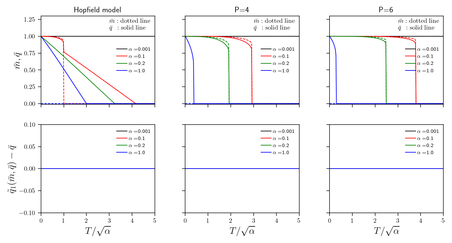
Figure 1: RS overlap $\bar{q}$ (top row) and the difference between $\tilde{q}_{1}({\color[rgb]{0,0,0}{\bar{m}},\,}\bar{q})$ and $\bar{q}$ (bottom row) versus the scaled parameter $T/\sqrt{\alpha}$, for different values of $\alpha$ (as shown in the legend), for the Hopfield model (left) and Hebbian networks with $P$-node interactions, for $P=4$ (mid) and $P=6$ (right).

While this limit is a priori unjustified, as $\bar{q}$ and $\tilde{q}_{1}({\color[rgb]{0,0,0}{\bar{m}},\,}\bar{q})$ should be solved from the self-consistency equations (9) and (25), respectively, one can check numerically that the solutions of these equations are virtually indistinguishable for any temperature (see Fig. 1, left panel), and the resulting RS instability line is almost identical to the AT line derived in coolen2001statistical , see Fig. 2 (left panel). Small deviations can be appreciated in the retrieval region (see right panel), but these are likely due to numerical precision.

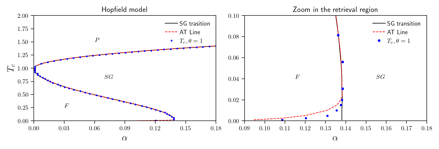
Figure 2: RS instability line (i.e. $T_{c}$ versus $\alpha$) obtained via our method (blue crosses) and the AT line obtained in the limit $\tilde{q}_{1}({\color[rgb]{0,0,0}{\bar{m}},\,}\bar{q})\to\bar{q}$ (red dashed curve), for the Hopfield model model. The several branches separate the paramagnetic (P), spin-glass (SG) and retrieval (M) region. The black curve show the critical temperature $T^{\star}$ at which $\bar{q}$ becomes non-zero within the RS theory, i.e. the spin-glass (SG) transition.

As our method does not rely on the assumption $\tilde{q}_{1}({\color[rgb]{0,0,0}{\bar{m}},\,}\bar{q})\to\bar{q}$, it provides a more general approach than the one originally devised by de Almeida and Thouless, that can be carried over to systems with discontinuous phase transitions, where $\bar{q}_{1}$ differs from $\bar{q}_{0}$ even at the onset of the RS instability, implying $\tilde{q}_{1}({\color[rgb]{0,0,0}{\bar{m}},\,}\bar{q})\neq\bar{q}$.

Before concluding this section, we note that, although we have disregarded the limit $\theta\to 0$ as lacking physical interpretation, such limit is still well defined mathematically and one may ask what would be the outcome of a similar analysis carried out in this limit. We will perform such analysis in Appendix B. Intriguingly, we find that the analysis for $\theta\to 0$ gives the same instability line as the analysis for $\theta\to 1$, in all the models we considered, except in the spherical $P$-spin model. Reassuringly, in the latter case, the analysis at $\theta\to 0$ leads to a lower temperature for the RS instability, confirming that the limit $\theta\to 1$ gives the physical transition and it is therefore the relevant one.

3 Hebbian networks with $P$-node interactions

In this section we consider generalizations of the Hopfield model, where neurons interact in P-tuples of even $P\geq 4$ (rather than pairwise, i.e. $P=2$). Such networks were shown to store many more patterns than the number of their nodes, so they work as dense associative memories HopKro1 . They are also known to be dual to deep neural networks Fachechi1 ; Albanese2021 and to exhibit information processing capabilities that are forbidden in shallow networks, such as the existence of a region in the parameter space where they can retrieve patterns although these are overshadowed by the noise Barra-PRLdetective . As before, we consider a network of $N$ interacting Ising neurons $\sigma_{i}\in\{1,-1\}$, with $K$ stored patterns $\bm{\xi}^{\mu}$ and $P$-node interactions $J_{i_{1}\ldots i_{P}}=\frac{1}{P!}\sum_{\mu=1}^{K}\xi^{\mu}_{i_{1}}\ldots\xi^{\mu}_{i_{P}}$. The Hamiltonian of this model can be written as

$${H_{N}(\bm{\sigma}|\bm{\xi})=-\dfrac{N^{1-P}}{P!}\sum_{\mu=1}^{K}\sum_{i_{1},\ldots,i_{P}}\xi^{\mu}_{i_{1}}\ldots\xi^{\mu}_{i_{P}}\sigma_{i_{1}}\ldots\sigma_{i_{P}}}$$ (35)

The order parameters are still the Mattis magnetization $m$ and the two-replicas overlap $q$, as introduced in (4), with their RS distributions given in (6) and (7) and their 1RSB generalizations given in (12) and (11). The quenched free-energy in RS assumption is (see Gardner )

$$-\beta^{{}^{\prime}}f_{RS}({\bar{m}},\bar{q}|\beta^{{}^{\prime}},\alpha)= \ln 2-\dfrac{{\beta^{{}^{\prime}}}}{2}(P-1){\bar{m}}^{P}+\dfrac{{\beta^{{}^{\prime}}}^{2}\alpha}{4}(1-\bar{q}^{P})-\dfrac{{\beta^{{}^{\prime}}}^{2}\alpha P}{4}\bar{q}^{P-1}(1-\bar{q})$$

$$+\mathbb{E}\ln\cosh\left(\beta^{{}^{\prime}}\dfrac{P}{2}{\bar{m}}^{P-1}+\beta^{{}^{\prime}}z\sqrt{\alpha\dfrac{P}{2}\bar{q}^{P-1}}\right)$$ (36)

with $\beta^{{}^{\prime}}:=2\beta/P!$, where $\beta$ is the inverse temperature and $\alpha=\lim_{N\to\infty}K/N^{P-1}$ is the network load. $\mathbb{E}$ is the average w.r.t. the standard Gaussian random variable $z$, and $\bar{q}$ and ${\bar{m}}$ satisfy the self-consistency equations:

$${\bar{m}}=\mathbb{E}\tanh\left(\beta^{{}^{\prime}}\dfrac{P}{2}{\bar{m}}^{P-1}+\beta^{{}^{\prime}}\sqrt{\alpha\dfrac{P}{2}\bar{q}^{P-1}}z\right),$$

$$\bar{q}=\mathbb{E}\tanh^{2}\left(\beta^{{}^{\prime}}\dfrac{P}{2}{\bar{m}}^{P-1}+\beta^{{}^{\prime}}\sqrt{\alpha\dfrac{P}{2}\bar{q}^{P-1}}z\right).$$ (37)

On the other hand, the quenched free-energy within the 1RSB approximation (see Albanese2021 ), reads as

$$-\beta^{{}^{\prime}}f_{1RSB}({\bar{m}_{1}},\bar{q}_{1},\bar{q}_{0}|\beta^{{}^{\prime}},\alpha,\theta)= \ln 2-\dfrac{{\beta^{{}^{\prime}}}}{2}(P-1){\bar{m}_{1}}^{P}+\dfrac{{\beta^{{}^{\prime}}}^{2}\alpha}{4}\left[1-\theta\bar{q}_{0}^{P}+(\theta-1)\bar{q}_{1}^{P}\right]$$

$$-\dfrac{{\beta^{{}^{\prime}}}^{2}\alpha P}{4}\bar{q}_{1}^{P-1}-\dfrac{{\beta^{{}^{\prime}}}^{2}}{4}P\alpha\left[(\theta-1)\bar{q}^{P}_{1}-\theta\bar{q}_{0}^{P}\right]$$

$$+\dfrac{1}{\theta}\mathbb{E}_{1}\ln\mathbb{E}_{2}\cosh^{\theta}g(\beta^{{}^{\prime}},\alpha,{\bar{m}_{1}},\bar{q}_{0},\bar{q}_{1})$$ (38)

where $\mathbb{E}_{1}$, $\mathbb{E}_{2}$ are the average w.r.t. the standard normal random variables $z^{(1)}$ and $z^{(2)}$, respectively, and

$$g({\bar{m}_{1}},\bar{q}_{1},\bar{q}_{0}|\beta^{{}^{\prime}},\alpha)= \dfrac{\beta^{{}^{\prime}}P}{2}{\bar{m}_{1}}^{P-1}+\beta^{{}^{\prime}}z^{(1)}\sqrt{\dfrac{P}{2}\alpha\bar{q}_{0}^{P-1}}+\beta^{{}^{\prime}}z^{(2)}\sqrt{\dfrac{P}{2}\alpha\left(\bar{q}_{1}^{P-1}-\bar{q}_{0}^{P-1}\right)}.$$ (39)

In this approximation the self-consistency equations for the order parameter $\bar{q}_{1}$, $\bar{q}_{0}$ and ${\bar{m}}$ are as in (17), with the argument of the hyperbolic cosine and tangent replaced by (39). As before, for $\theta=1$, $\bar{q}_{0}=\bar{q}$ and the 1RSB expression for the quenched free-energy reduces to the RS one.

From now on, we imply the dependence of the functions on $\beta^{{}^{\prime}}$ and $\alpha$. Our objective is to prove that for $\theta$ close but away from one, the 1RSB quenched free-energy is smaller than its replica symmetric counterpart i.e. $f_{1RSB}({\color[rgb]{0,0,0}{\bar{m}_{1}},\,}\bar{q}_{1},\bar{q}_{0}|\theta)<f_{RS}({\color[rgb]{0,0,0}{\bar{m}},\,}\bar{q})$ above a critical value of the effective parameter $\sqrt{\alpha}\beta^{\prime}$. To this purpose, we proceed as in the Hopfield model: we expand, to the leading order in $\theta-1$, the 1RSB quenched free-energy around its RS expression, as shown in (21). Since the self-consistency equations also depend on $\theta$, we need to expand them too. Following the same steps as in the Hopfield model, we can write ${\bar{m}_{1}}$ as in (28) with $C({\bar{m}},\bar{q},{\color[rgb]{0,0,0}\tilde{q}_{1}({\bar{m}},\bar{q})})$ as in (125), where $\tilde{q}_{1}({\color[rgb]{0,0,0}{\bar{m}},\,}\bar{q})$ is the solution of the self-consistency equation

$$\bar{q}_{1} =\mathbb{E}_{1}\left[\dfrac{\mathbb{E}_{2}\cosh{g({\color[rgb]{0,0,0}{\bar{m}},\,}\bar{q}_{1},\bar{q})}\tanh^{2}{g({\color[rgb]{0,0,0}{\bar{m}},\,}\bar{q}_{1},\bar{q})}}{\mathbb{E}_{2}\cosh{g({\color[rgb]{0,0,0}{\bar{m}},\,}\bar{q}_{1},\bar{q})}}\right],$$ (40)

$\bar{q}_{0}$ as in (27), with $A({\color[rgb]{0,0,0}{\bar{m}_{1}},\,}\bar{q},\tilde{q}_{1}({\bar{m}},\bar{q}))$ given in (123), and $\bar{q}_{1}$ as given in (26) with $B({\color[rgb]{0,0,0}{\bar{m}},\,}\bar{q},\tilde{q}_{1}({\color[rgb]{0,0,0}{\bar{m}},\,}\bar{q}))$ given in (124). With the above expressions in hand, we can now calculate the derivative of $f_{\rm 1RSB}$ w.r.t. $\theta$ when $\theta=1$, as needed in (21)

$$K({\color[rgb]{0,0,0}{\bar{m}},\,}\tilde{q}_{1}({\color[rgb]{0,0,0}{\bar{m}},\,}\bar{q}),\bar{q}):=\partial_{\theta}(-\beta^{{}^{\prime}}f_{\rm 1RSB}({\color[rgb]{0,0,0}{\bar{m}_{1}},\,}\bar{q}_{1},\bar{q}_{0}|\theta))|_{\theta=1}$$

$$=-\dfrac{{\beta^{{}^{\prime}}}^{2}\alpha}{4}(P-1)[(\tilde{q}_{1}({\color[rgb]{0,0,0}{\bar{m}},\,}\bar{q}))^{P}-\bar{q}^{P}]-\dfrac{{\beta^{{}^{\prime}}}^{2}\alpha}{4}P[(\tilde{q}_{1}({\color[rgb]{0,0,0}{\bar{m}},\,}\bar{q}))^{P-1}-\bar{q}^{P-1}]$$

$$-\mathbb{E}\ln\cosh\left(\beta^{{}^{\prime}}\sqrt{\dfrac{P}{2}\bar{q}^{P-1}}z+\beta^{{}^{\prime}}{\bar{m}}^{P-1}\right)+\mathbb{E}_{1}\left[\dfrac{\mathbb{E}_{2}\cosh g({\color[rgb]{0,0,0}{\bar{m}},\,}\tilde{q}_{1}({\color[rgb]{0,0,0}{\bar{m}},\,}\bar{q}),\bar{q})\log\cosh g({\color[rgb]{0,0,0}{\bar{m}},\,}\tilde{q}_{1}({\color[rgb]{0,0,0}{\bar{m}},\,}\bar{q}),\bar{q})}{\mathbb{E}_{2}\cosh g({\color[rgb]{0,0,0}{\bar{m}},\,}\tilde{q}_{1}({\color[rgb]{0,0,0}{\bar{m}},\,}\bar{q}),\bar{q})}\right]$$ (41)

Again, we have that $K({\color[rgb]{0,0,0}{\bar{m}},\,}\bar{q},\bar{q})=0$, regardless of the value assigned to ${\bar{m}}$, (this follows from the fact that for $\theta=1$, $\bar{q}$ is an extremum of the free-energy). Next, we inspect the sign of $K({\color[rgb]{0,0,0}{\bar{m}},\,}\tilde{q}_{1}({\color[rgb]{0,0,0}{\bar{m}},\,}\bar{q}),\bar{q})$. To this purpose, we study $K({\color[rgb]{0,0,0}{\bar{m}},\,}\bar{q},x)$ for $x\in[0,\bar{q}]$ and locate its extrema, which are found from

$$\partial_{x}K({\color[rgb]{0,0,0}{\bar{m}},\,}\bar{q},x)= -\dfrac{{\beta^{{}^{\prime}}}^{2}\alpha}{4}(P-1)Px^{P-2}\left[x-\mathbb{E}_{1}\left[\dfrac{\mathbb{E}_{2}\sinh g({\color[rgb]{0,0,0}{\bar{m}},\,}\bar{q},x)\tanh g({\color[rgb]{0,0,0}{\bar{m}},\,}\bar{q},x)}{\mathbb{E}_{2}\cosh g({\color[rgb]{0,0,0}{\bar{m}},\,}\bar{q},x)}\right]\right]=0$$ (42)

as

$$x=\mathbb{E}_{1}\left[\dfrac{\mathbb{E}_{2}\cosh{g(x,\bar{q})}\tanh^{2}{g(x,\bar{q})}}{\mathbb{E}_{2}\cosh{g(x,\bar{q})}}\right]\equiv\tilde{q}_{1}({\color[rgb]{0,0,0}{\bar{m}},\,}\bar{q})$$ (43)

where the last equality follows from (40). Under the assumption that the extremum $x=\tilde{q}_{1}({\color[rgb]{0,0,0}{\bar{m}},\,}\bar{q})$ is global in the domain considered and reasoning as in the Hopfield case, we have that $K({\color[rgb]{0,0,0}{\bar{m}},\,}\tilde{q}_{1}({\color[rgb]{0,0,0}{\bar{m}},\,}\bar{q}),\bar{q})>0$ if $x=\tilde{q}_{1}({\color[rgb]{0,0,0}{\bar{m}},\,}\bar{q})$ is a maximum and $K({\color[rgb]{0,0,0}{\bar{m}},\,}\tilde{q}_{1}({\color[rgb]{0,0,0}{\bar{m}},\,}\bar{q}),\bar{q})<0$ if it is a minimum. In particular, if

$$\partial^{2}_{x}K({\color[rgb]{0,0,0}{\bar{m}},\,}\bar{q},x)|_{x=\tilde{q}_{1}({\color[rgb]{0,0,0}{\bar{m}},\,}\bar{q})}= -\dfrac{{\beta^{{}^{\prime}}}^{2}\alpha(P-1)P}{4}(\tilde{q}_{1}({\color[rgb]{0,0,0}{\bar{m}},\,}\bar{q}))^{P-2}$$

$$\cdot\left\{1-\dfrac{{\beta^{{}^{\prime}}}^{2}\alpha}{2}(P-1)P(\tilde{q}_{1}({\color[rgb]{0,0,0}{\bar{m}},\,}\bar{q}))^{P-2}\mathbb{E}_{1}\left[\dfrac{\mathbb{E}_{2}\textnormal{sech}^{3}g({\color[rgb]{0,0,0}{\bar{m}},\,}\tilde{q}_{1}({\color[rgb]{0,0,0}{\bar{m}},\,}\bar{q}),\bar{q})}{\mathbb{E}_{2}\cosh g({\color[rgb]{0,0,0}{\bar{m}},\,}\tilde{q}_{1}({\color[rgb]{0,0,0}{\bar{m}},\,}\bar{q}),\bar{q})}\right]\right\}$$ (44)

is positive, $K({\color[rgb]{0,0,0}{\bar{m}},\,}\tilde{q}_{1}({\color[rgb]{0,0,0}{\bar{m}},\,}\bar{q}),\bar{q})<0$ and $f_{1RSB}<f_{RS}$. This happens when the expression in the curly brackets of the equation above is negative, i.e. when the parameter $\alpha{\beta^{{}^{\prime}}}^{2}$ satisfies the inequality

$$\dfrac{{\beta^{{}^{\prime}}}^{2}\alpha}{2}(P-1)P(\tilde{q}_{1}({\color[rgb]{0,0,0}{\bar{m}},\,}\bar{q}))^{P-2}\mathbb{E}_{1}\left[\dfrac{\mathbb{E}_{2}\textnormal{sech}^{3}g({\color[rgb]{0,0,0}{\bar{m}},\,}\bar{q},\tilde{q}_{1}({\color[rgb]{0,0,0}{\bar{m}},\,}\bar{q}))}{\mathbb{E}_{2}\cosh g({\color[rgb]{0,0,0}{\bar{m}},\,}\bar{q},\tilde{q}_{1}({\color[rgb]{0,0,0}{\bar{m}},\,}\bar{q}))}\right]>1.$$ (45)

As noted in Albanese2021 ; glassy , Hebbian networks with $P$-node interactions are equivalent to Ising $P$-spin models under a suitable rescaling of the temperature $\beta^{{}^{\prime}}\sqrt{\alpha}\to\beta^{\prime}$. With this rescaling, (45) retrieves indeed the RS instability line of the Ising P-spin model, that we have for completeness derived in Appendix A, using our method (see eq. (75)). In the limit $\tilde{q}_{1}({\color[rgb]{0,0,0}{\bar{m}},\,}\bar{q})\to\bar{q}$, (75) retrieves the AT line of the Ising $P$-spin model gardner1985spin . In Fig. 1 (mid and right panels) we plot the difference between $\tilde{q}_{1}({\color[rgb]{0,0,0}{\bar{m}},\,}\bar{q})$ and $\bar{q}$ for Hebbian networks with $P$-node interactions (obtained solving numerically the self-consistency equations (40) and (37)) as a function of the scaled parameter $T/\sqrt{\alpha}$, for different values of $\alpha$. As for the Hopfield model, we find that $\tilde{q}_{1}({\color[rgb]{0,0,0}{\bar{m}},\,}\bar{q})$ is indistinguishable from $\bar{q}$, hence the limit $\tilde{q}_{1}({\color[rgb]{0,0,0}{\bar{m}},\,}\bar{q})\to\bar{q}$ can be justified a posteriori.

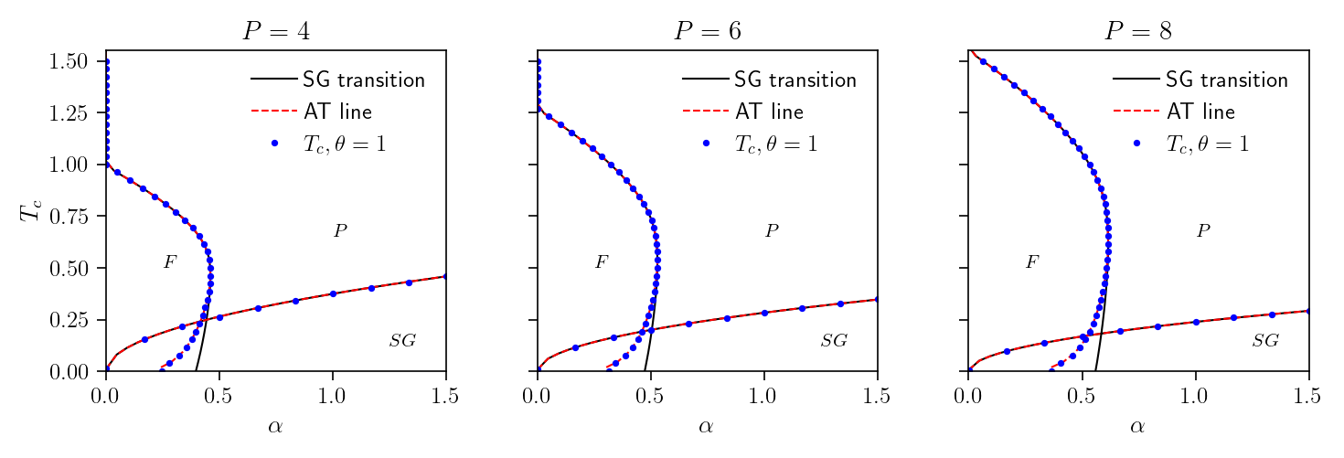
Figure 3: RS instability line (i.e. $T_{c}$ versus $\alpha$) obtained via our method, i.e. by expanding the free-energy around $\theta=1$ (blue dots) and the AT line obtained in the limit $\tilde{q}_{1}({\color[rgb]{0,0,0}{\bar{m}},\,}\bar{q})\to\bar{q}$ (red curve), for the Hebbian network with $P$-node interactions, with $P=2,4,6$ from left to right. The black curves show the critical temperature $T^{\star}$ at which $\bar{q}$ becomes non-zero within the RS theory, i.e. the spin-glass (SG) transition.

In Fig. 3 we show the RS instability lines resulting from our method and the classic AT line obtained in the limit $\tilde{q}_{1}({\color[rgb]{0,0,0}{\bar{m}},\,}\bar{q})\rightarrow\bar{q}$, for different values of $P$. The two lines coincides for all values of $P$. As explained earlier, we could have expanded the free-energy around $\theta=0$ (as opposed to $\theta=1$). In Appendix B we show that such analysis leads to the same line.

4 Discussion

In this work we proposed a simple and systematic method to derive the critical line in the parameter space $(\alpha,\beta)$, below which the 1RSB expression for the free-energy is smaller than the RS expression, in Hebbian neural networks. The same analysis for spin-glass models is carried out in appendix A. For the Hopfield model, our approach recovers the critical line obtained by Coolen using the AT approach coolen2001statistical as a special limit. Similarly, we recover the known AT lines of all the spin-glass models considered in the appendix, in the same limit, showing that our method provides a generalization of the approach originally devised by de Almeida and Thouless. Owing to its simplicity, our method allows for straightforward application to Hebbian networks with multi-node interactions, for which the AT-line was unknown.

The key idea of our method is to regard the 1RSB theory, which assumes two delta-peaks in the overlap distribution $P(q)$, located at $\bar{q}_{1}$ and $\bar{q}_{0}<\bar{q}_{1}$, with weights $1-\theta$ and $\theta$, respectively, as departing continuously from the RS theory, which assumes only one peak at $\bar{q}$. This leads us to assume that at the onset of the RS instability, the 1RSB overlap distribution is dominated by one peak, so that either $\theta\to 0$ or $\theta\to 1$. Then, consistency with the RS theory requires either $\lim_{\theta\to 0}\bar{q}_{1}\!=\!\bar{q}$ or $\lim_{\theta\to 1}\bar{q}_{0}\!=\!\bar{q}$. As the physical interpretation of RS breaking suggests that the mutual overlap between 1RSB states should be equal to the self-overlap of the RS states, we regard the 1RSB theory as a continuous variation of the RS theory, when the parameter $\theta$ is decreased from one. Crucially, we do not make any assumption on the location of the peaks of the 1RSB theory, which are fixed by the 1RSB self-consistency equations. We then compare the 1RSB and the RS free-energies when $\theta$ (the only free-parameter in our analysis) is close to one, by performing simple expansions to linear orders in $\theta-1$. In doing so, we solely require that $f_{1RSB},\bar{q}_{1},\bar{q}_{0}$ and ${\bar{m}_{1}}$ are differentiable up to the first order in a neighborhood of $\theta\!=\!1$ and that the derivative of $f_{1RSB}$ exists at $\theta=1$.

Although our method is similar in spirit to the one introduced by Toninelli in toninelli2002almeida , there is a crucial difference, in that the latter relies on the assumption $\bar{q}_{1}\to\bar{q}$, which is, in our view, unjustified a priori. In fact, while $\bar{q}_{0}=\bar{q}$ for $\theta=1$, $\bar{q}_{1}$ may differ from $\bar{q}$, even in the limit $\theta\to 1$. This consideration also leads to a departure of our approach from the method originally devised by de Almeida and Thouless, which relies on a variation of the RS free-energy as the order parameters are varied continuously around their RS values. In contrast, we study the variation of the RS free-energy as the statistical weight of the order parameters is varied continuously (rather than the actual value of the order parameters). This approach allows us to determine the instability line of the RS theory also in spin-glass models which exhibit a discontinuous phase transition. As a prototypical example of this class of models, we consider in Appendix A the spherical $P$-spin model Crisanti-RSB .

In conclusion, in this work we have presented a new method to find the instability line of the RS approximation. A compelling advantage of our method, when compared to the approach by de Almeida and Thouless de1978stability , is that it does not require to compute the full eigenspectrum of the Hessian of the quadratic fluctuations of the free-energy around its RS value and it does not rely on the availability of an “ansatz-free” expression for the free-energy. This makes the computations easier and affordable also for neural networks. The method still requires the availability of explicit expressions for the RS and 1RSB free-energies, which however can be computed using different techniques (e.g. Guerra’s interpolation) in addition to the replica trick. Our approach can in principle be extended to compute the stability of the $k$-RSB solution, expanding the corresponding $k\!+\!1$-RSB free-energy, provided one has an explicit expression for the two. For example, it would be interesting to see whether the well-known transition from $1$RSB to full-RSB occurring at the Gardner temperature gardner1985spin in the Ising $P$-spin model can be recovered within our approach, by studying the stability of the $2$RSB solution. In addition, in recent years there has been a boost of renewed interest in mixed $P$-spherical models, as introduced in AnnibaleGualdiCavagna04 ; CrisantiLeuzzi04 , as they have been shown to display unexpected dynamical behaviour FolenaFranzTersenghi20 and new types of spin-glass phases CrisantiLeuzzi05 , TonoloNieddaGradenigo as well as for their relevance to the modelling of random lasers Antenucci15 ; Antenucci15b ; Antenucci15c ; Antenucci16 ; Antenucci21 . These models similarly display transitions from $1$RSB to full-RSB and would be good lab systems to test extensions of our theory. Another interesting avenue for future work would be a generalization of the $1$-RSB scheme, which does not assume the Mattis magnetization to be self-averaging. Preliminary work in AABO-JPA2020 suggests that the RS assumption is not the right approximation for Mattis magnetization.

Finally, an attractive perspective would be to apply our approach to predict the onset of ergodicity breaking in systems with sparse interactions. In such systems, the free-energy is typically expressed, already at the simplest RS level, in terms of order-parameter functions to be determined self-consistently. At 1RSB level, recursive equations for functional distributions of such functions must be solved. Working out the fluctuations of ansatz-free free-energies around their RS value, as it would be required by the de Almeida and Thouless approach would be unfeasible and no similar approach has been proposed to date. An alternative approach has been devised in Thouless86 , for the Bethe lattice with regular degrees, however it strongly relies on the assumptions of homogeneity in the network nodes and large degrees. We envisage that, owing to its simplicity, our method may carry over to more general sparse systems, where it would require an expansion of the functional 1RSB self-consistency equation to linear orders around the RS equation, which should be feasible.

Appendix A Applications to Spin-glasses models

In this appendix, we derive the critical line for the instability of the RS theory for three archetypical spin-glass models, namely the SK model, the Ising $P$-spin and the spherical $P$-spin model, using the technique developed in the main text. In all cases, we will recover the AT lines known in the literature for the three models, in a specific limit, confirming the validity and higher generality of our approach.

A.1 Sherrington-Kirkpatrick Model

The Sherrington-Kirkpatrick (SK) model sherrington1975solvable is a system of $N$ Ising spins $\sigma_{i}\in\{\pm 1\}$ interacting via symmetric pairwise interactions $J_{ij}$ which are i.i.d. Gaussian variables with zero average and variance $J^{2}/N$. The Hamiltonian of the model is

$$H_{N}(\bm{\sigma}|J):=-\dfrac{1}{2}\sum_{i,j}^{N,N}J_{ij}\sigma_{i}\sigma_{j}$$ (46)

and the order parameter is the two-replica overlap $q$ as defined in (4). The quenched free-energy in RS assumption is sherrington1975solvable

$$-\beta f_{RS}(\bar{q}|\beta,J)=\ln 2+\dfrac{\beta^{2}J^{2}}{4}(1-\bar{q})^{2}+\mathbb{E}\left[\ln\cosh\left(\beta J\sqrt{\bar{q}}z\right)\right]$$ (47)

where $\mathbb{E}$ is the average w.r.t. the Gaussian variable $z$ and the order parameter $\bar{q}$ fulfills the self-consistency equation

$$\bar{q}=\mathbb{E}\tanh^{2}\left(\beta J\sqrt{\bar{q}}z\right).$$ (48)

The 1RSB approximation of the quenched free-energy is (see e.g. nishimori2001statistical )

$$-\beta f_{1RSB}(\bar{q}_{1},\bar{q}_{0}|\beta,J,\theta)= \ln 2+\dfrac{\beta^{2}J^{2}}{2}(1-\bar{q}_{1})+\dfrac{1}{\theta}\mathbb{E}_{1}\left[\ln\mathbb{E}_{2}\cosh^{\theta}g(\beta,J,\bar{q}_{1},\bar{q}_{0})\right]$$

$$-\dfrac{\beta^{2}J^{2}}{4}\left[1-\bar{q}_{1}^{2}+\theta(\bar{q}_{1}^{2}-\bar{q}_{0}^{2})\right],$$ (49)

where

$$g(\bar{q}_{1},\bar{q}_{0}|\beta,J)=\beta J\sqrt{\bar{q}_{1}-\bar{q}_{0}}z^{(2)}+\beta J\sqrt{\bar{q}_{0}}z^{(1)}$$ (50)

and $\mathbb{E}_{1}$, $\mathbb{E}_{2}$ are the average w.r.t. the standard Gaussian variables $z^{(1)}$ and $z^{(2)}$, respectively. From now on, we imply the dependence of $g$, $f_{RS}$ and $f_{1RSB}$ on $\beta$ and $J$. The order parameters $\bar{q}_{0}$ and $\bar{q}_{1}$ fulfill the following self-consistency equations

$$\bar{q}_{1} =\mathbb{E}_{1}\left[\dfrac{\mathbb{E}_{2}\cosh^{\theta}g(\bar{q}_{1},\bar{q}_{0})\tanh^{2}g(\bar{q}_{1},\bar{q}_{0})}{\mathbb{E}_{2}\cosh^{\theta}g(\bar{q}_{1},\bar{q}_{0})}\right],$$

$$\bar{q}_{0} =\mathbb{E}_{1}\left[\dfrac{\mathbb{E}_{2}\cosh^{\theta}g(\bar{q}_{1},\bar{q}_{0})\tanh g(\bar{q}_{1},\bar{q}_{0})}{\mathbb{E}_{2}\cosh^{\theta}g(\bar{q}_{1},\bar{q}_{0})}\right]^{2}.$$ (51)

Noting that $\lim_{\theta\to 1}\bar{q}_{0}=\bar{q}$ and $f_{1RSB}(\bar{q}_{1},\bar{q}_{0}|\theta=1)=f_{RS}(\bar{q})$, our objective is to expand the 1RSB quenched free-energy for $\theta\simeq 1$. To this purpose, we expand the self-consistency equations for $\bar{q}_{0}$ and $\bar{q}_{1}$ to linear order in $\theta-1$. Proceding as in the Hopfield model, we get

$$\bar{q}_{0} =\bar{q}+(\theta-1)A(\bar{q},\tilde{q}_{1}(\bar{q}))$$ (52)

$$\bar{q}_{1} =\tilde{q}_{1}(\bar{q})+(\theta-1)B(\bar{q},\tilde{q}_{1}(\bar{q}))$$ (53)

where $\tilde{q}_{1}(\bar{q})$ solves the self-consistency equation

$$\bar{q}_{1}=\mathbb{E}_{1}\left\{\dfrac{\mathbb{E}_{2}\cosh g(\bar{q}_{1},\bar{q})\tanh^{2}g(\bar{q}_{1},\bar{q})}{\mathbb{E}_{2}\cosh g(\bar{q}_{1},\bar{q})}\right\}$$ (54)

and $A(\bar{q}_{0},\bar{q}_{1})$ and $B(\bar{q}_{0},\bar{q}_{1})$ are given in (129) and (130), respectively. Next, we derive w.r.t. $\theta$ the 1RSB free-energy (49) where we replace $\bar{q}_{0}$ and $\bar{q}_{1}$ with (52), (53), obtaining

$$\partial_{\theta}(-\beta f_{1RSB}(\bar{q}_{1},\bar{q}_{0},|\theta))= -\dfrac{{\beta}^{2}J^{2}}{4}\left[(\tilde{q}_{1}(\bar{q}))^{2}-\bar{q}^{2}\right]-\dfrac{1}{\theta^{2}}\mathbb{E}_{1}\ln\mathbb{E}_{2}\cosh^{\theta}g(\tilde{q}_{1}(\bar{q}),\bar{q})$$

$$-\dfrac{{\beta}^{2}J^{2}}{2}B(\tilde{q}_{1}(\bar{q}),\bar{q})\bar{q}+\dfrac{1}{\theta}\mathbb{E}_{1}\left[\dfrac{\mathbb{E}_{2}\cosh^{\theta}g(\tilde{q}_{1}(\bar{q}),\bar{q})\log\cosh g(\tilde{q}_{1}(\bar{q}),\bar{q})}{\mathbb{E}_{2}\cosh^{\theta}g(\tilde{q}_{1}(\bar{q}),\bar{q})}\right]$$

$$+\dfrac{{\beta}^{2}J^{2}}{2}B(\tilde{q}_{1}(\bar{q}),\bar{q})\theta\mathbb{E}_{1}\left[\dfrac{\mathbb{E}_{2}\cosh^{\theta}g(\tilde{q}_{1}(\bar{q}),\bar{q})\tanh g(\tilde{q}_{1}(\bar{q}),\bar{q})}{\mathbb{E}_{2}\cosh^{\theta}g(\tilde{q}_{1}(\bar{q}),\bar{q})}\right]^{2},$$ (55)

which for $\theta=1$, using (48) and similar manipulations to those used in (19), evaluates to

$$K(\tilde{q}_{1}(\bar{q}),\bar{q}):=\partial_{\theta}(-\beta f_{1RSB} (\bar{q}_{1},\bar{q}_{0},|\theta))|_{\theta=1}=-\dfrac{{\beta}^{2}J^{2}}{4}\left[(\tilde{q}_{1}(\bar{q}))^{2}-\bar{q}^{2}\right]-\dfrac{{\beta}^{2}J^{2}}{2}(\tilde{q}_{1}(\bar{q})-\bar{q})$$

$$-\mathbb{E}\ln\cosh\left(\beta\sqrt{\bar{q}}z\right)+\mathbb{E}_{1}\left[\dfrac{\mathbb{E}_{2}\cosh g(\tilde{q}_{1}(\bar{q}),\bar{q})\log\cosh g(\tilde{q}_{1}(\bar{q}),\bar{q})}{\mathbb{E}_{2}\cosh g(\tilde{q}_{1}(\bar{q}),\bar{q})}\right].$$ (56)

We then study the sign of (56), where $\bar{q}$ and $\tilde{q}_{1}(\bar{q})$ are the solutions of the self-consistency equations (48) and (54), respectively. To this purpose, it is useful to study the behaviour of the function $K(\bar{q},x)$ for $x\in[0,\bar{q}]$. For $x=\bar{q}$, we have $K(\bar{q},\bar{q})=0$, while the extremum of $K(\bar{q},x)$ is found from

$$\partial_{x}K(x,\bar{q}) =-\dfrac{{\beta}^{2}J^{2}}{2}x+\dfrac{{\beta}^{2}J^{2}}{2}\mathbb{E}_{1}\left[\dfrac{\mathbb{E}_{2}\sinh g(x,\bar{q})\tanh g(x,\bar{q})}{\mathbb{E}_{2}\cosh g(x,\bar{q})}\right]=0,$$ (57)

as

$$x=\mathbb{E}_{1}\left[\dfrac{\mathbb{E}_{2}\sinh g(x,\bar{q})\tanh g(x,\bar{q})}{\mathbb{E}_{2}\cosh g(x,\bar{q})}\right]\equiv\tilde{q}_{1}(\bar{q})$$ (58)

via Eq. (54). Given that $K(\bar{q},x)$ vanishes for $x=\bar{q}$, if the extremum $x=\tilde{q}_{1}(\bar{q})$ is global in the domain considered, we must have that $K(\tilde{q}_{1}(\bar{q}),\bar{q})>0$ if $x=\tilde{q}_{1}(\bar{q})$ is a maximum and $K(\tilde{q}_{1}(\bar{q}),\bar{q})<0$ if $x=\tilde{q}_{1}(\bar{q})$ is a minimum. Therefore, if

$$\partial_{x}^{2}K(x,\bar{q})|_{x=\tilde{q}_{1}(\bar{q})}= -\dfrac{{\beta}^{2}J^{2}}{2}\left(1-\dfrac{{\beta}^{2}J^{2}}{2}\mathbb{E}_{1}\left[\dfrac{\mathbb{E}_{2}\textnormal{sech}^{3}g(\tilde{q}_{1}(\bar{q}),\bar{q})}{\mathbb{E}_{2}\cosh g(\tilde{q}_{1}(\bar{q}),\bar{q})}\right]\right)$$ (59)

is positive, $K(\bar{q},\tilde{q}_{1}(\bar{q}))$ is negative, so the RS theory becomes unstable for

$$1-\dfrac{{\beta}^{2}J^{2}}{2}\mathbb{E}_{1}\left[\dfrac{\mathbb{E}_{2}\textnormal{sech}^{3}\ g(\tilde{q}_{1}(\bar{q}),\bar{q})}{\mathbb{E}_{2}\cosh g(\tilde{q}_{1}(\bar{q}),\bar{q})}\right]<0.$$ (60)

We note that for $\tilde{q}_{1}(\bar{q})\to\bar{q}$, such condition retrieves the well-known AT line de1978stability

$$1-{\beta^{2}J^{2}}\mathbb{E}\left(\dfrac{1}{\cosh^{4}\left(\beta J\sqrt{\bar{q}}z\right)}\right)<0.$$ (61)

By numerically solving the self-consistency equations (48) and (54), we can verify that $\tilde{q}_{1}(\bar{q})=\bar{q}$ for all temperatures, hence this limit can be justified a posteriori for the SK model (see Fig. 4, left panel). We anticipate that this remains true for the Ising $P$-spin model analysed in the next section.

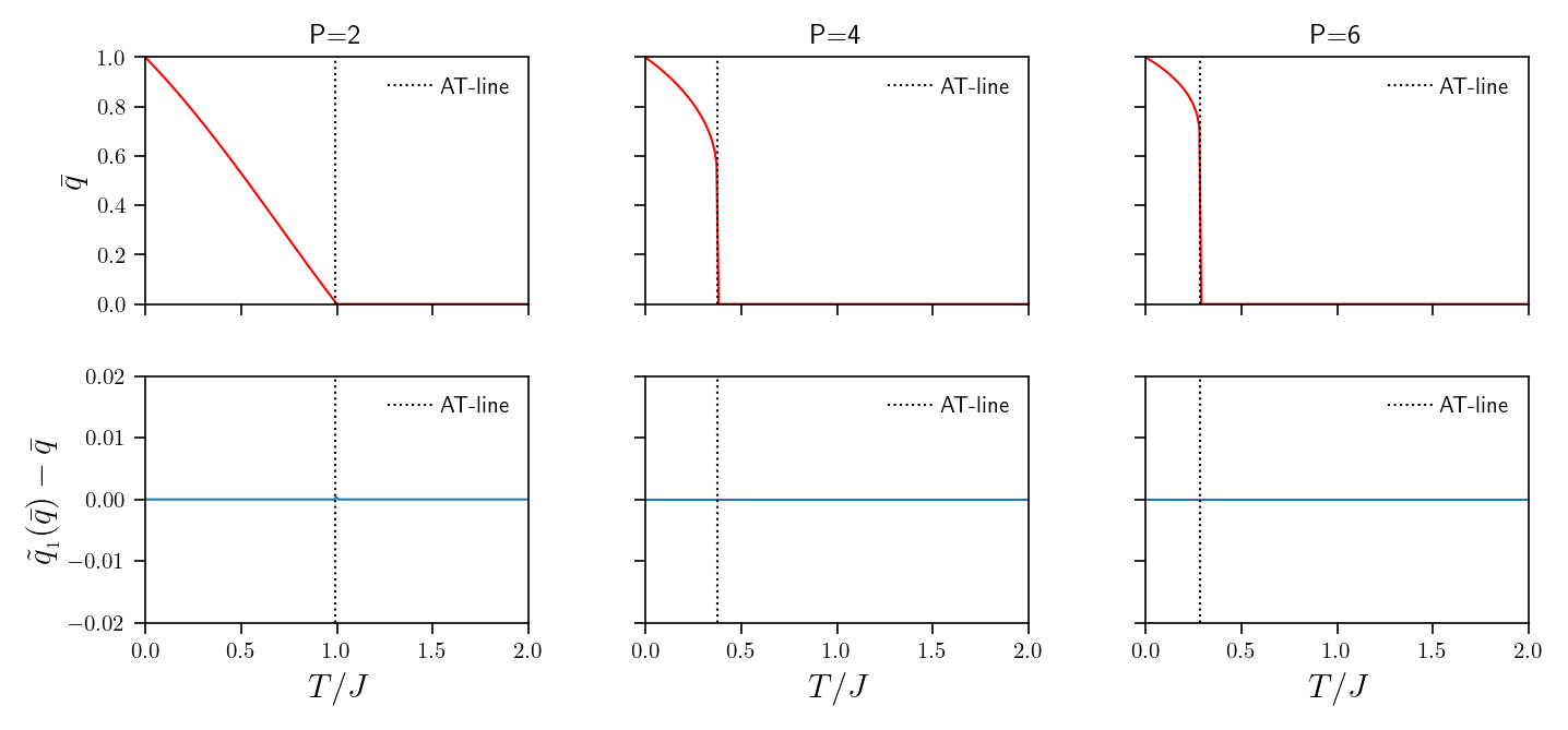
Figure 4: RS overlap $\bar{q}$ (top) and difference between $\bar{q}_{1}(\bar{q})$ and $\bar{q}$ (bottom) versus the ratio $T/J$, for the SK model (left) and the Ising $P$-spin model, with $P=4$ (mid) and $P=6$ (right panel). The dotted vertical line marks the onset of the RS instability.

A.2 The Ising P-spin model

In this section, we consider a system of $N$ Ising spins $\sigma_{i}=\pm 1$, $i=1,\ldots,N$ governed by the Hamiltonian

$$H_{N}(\bm{\sigma}|J) =-\dfrac{1}{N^{P-1}P!}\sum_{i_{1},\ldots,i_{P}=1,\ldots,1}^{N,\ldots,N}J_{i_{1},\ldots,i_{P}}\sigma_{i_{1}}\ldots\sigma_{i_{P}}$$ (62)

where $J_{i_{1},\ldots,i_{P}}$ are Gaussian i.i.d. variables, $J_{i_{1},\ldots,i_{P}}\sim\mathcal{N}(0,J^{2})$. As in the previous cases, the order parameter of the model is the two-replica overlap $q$ defined in (4). The quenched free-energy in RS assumption, at inverse temperature $\beta$ reads as gardner1985spin

$$-\beta^{{}^{\prime}}f_{RS}(\bar{q}|\beta^{\prime},J)= \ln 2+\dfrac{{\beta^{{}^{\prime}}}^{2}J^{2}}{4}[1-P\bar{q}^{P-1}+(P-1)\bar{q}^{P}]+\mathbb{E}\ln\cosh\left(\beta^{{}^{\prime}}Jz\sqrt{\dfrac{P}{2}\bar{q}^{P-1}}\right)$$ (63)

where $\beta^{{}^{\prime}}=2\beta/P!$, $\mathbb{E}$ is the average w.r.t. the Gaussian variable $z$ and $\bar{q}$ fulfills the following self-consistency equation:

$$\bar{q}=\mathbb{E}\tanh^{2}\left(\beta^{{}^{\prime}}Jz\sqrt{\dfrac{P}{2}\bar{q}^{P-1}}\right).$$ (64)

The 1RSB expression of the quenched free-energy in the thermodynamic limit is gardner1985spin

$$-\beta^{{}^{\prime}}f_{1RSB}(\bar{q}_{1},\bar{q}_{0}|\beta^{\prime},J,\theta)= \ln 2+\dfrac{{\beta^{{}^{\prime}}}^{2}J^{2}}{4}\left[1-P\bar{q}_{1}^{P-1}+(P-1)\bar{q}_{1}^{P}\right]$$

$$+\dfrac{1}{\theta}\mathbb{E}_{1}\ln\mathbb{E}_{2}\cosh^{\theta}g(\beta^{\prime},J,\bar{q}_{1},\bar{q}_{0})-\dfrac{{\beta^{{}^{\prime}}}^{2}J^{2}}{4}(P-1)\theta(\bar{q}_{1}^{P}-\bar{q}_{0}^{P})$$ (65)

where

$$g(\beta^{\prime},J,\bar{q}_{1},\bar{q}_{0})=\beta^{{}^{\prime}}Jz^{(1)}\sqrt{\dfrac{P}{2}\bar{q}_{0}^{P-1}}+\beta^{{}^{\prime}}Jz^{(2)}\sqrt{\dfrac{P}{2}(\bar{q}_{1}^{P-1}-\bar{q}_{0}^{P-1})},$$ (66)

$\mathbb{E}_{1}$, $\mathbb{E}_{2}$ are the average w.r.t. the standard Gaussian variables $z^{(1)}$ and $z^{(2)}$ and $\bar{q}_{0},\ \bar{q}_{1}$ fulfill the following self-consistency equations

$$\begin{array}[]{lll}\bar{q}_{1}&=\mathbb{E}_{1}\left[\dfrac{\mathbb{E}_{2}\cosh^{\theta}g(\beta^{\prime},J,\bar{q}_{1},\bar{q}_{0})\tanh^{2}g(\beta^{\prime},J,\bar{q}_{1},\bar{q}_{0})}{\mathbb{E}_{2}\cosh^{\theta}g(\beta^{\prime},J,\bar{q}_{1},\bar{q}_{0})}\right],\\ \\ \bar{q}_{0}&=\mathbb{E}_{1}\left[\dfrac{\mathbb{E}_{2}\cosh^{\theta}g(\beta^{\prime},J,\bar{q}_{1},\bar{q}_{0})\tanh(\beta^{\prime},J,\bar{q}_{1},\bar{q}_{0})}{\mathbb{E}_{2}\cosh^{\theta}g(\beta^{\prime},J,\bar{q}_{1},\bar{q}_{0})}\right]^{2}.\end{array}$$ (67)

From now on, we imply the dependence of $g$ and of the RS and 1RSB quenched free energies $f_{RS}$, $f_{1RSB}$ on $\beta^{\prime}$ and $J$. The aim is to prove that the 1RSB approximation of the quenched free-energy is smaller than the replica symmetric one, above a critical value of the parameter $\beta^{\prime}J$.

As before, we note that $\lim_{\theta\to 1}\bar{q}_{0}=\bar{q}$ and $f_{1RSB}(\bar{q}_{1},\bar{q}_{0}|\theta=1)=f_{RS}(\bar{q})$ and we aim at expanding the 1RSB quenched free-energy for $\theta\simeq 1$. To this purpose, we first expand the self-consistency equations for $\bar{q}_{0}$ and $\bar{q}_{1}$ to linear order in $\theta-1$, to obtain

$$\bar{q}_{0} =\bar{q}+(\theta-1)A(\bar{q},\tilde{q}_{1}(\bar{q}))$$ (68)

$$\bar{q}_{1} =\tilde{q}_{1}(\bar{q})+(\theta-1)B(\bar{q},\tilde{q}_{1}(\bar{q}))$$ (69)

where $\tilde{q}_{1}(\bar{q})$ solves the self-consistency equation

$$\bar{q}_{1}=\mathbb{E}_{1}\left\{\dfrac{\mathbb{E}_{2}\cosh g(\bar{q}_{1},\bar{q})\tanh^{2}g(\bar{q}_{1},\bar{q})}{\mathbb{E}_{2}\cosh g(\bar{q}_{1},\bar{q})}\right\}$$ (70)

and $A(\bar{q}_{0},\bar{q}_{1})$ and $B(\bar{q}_{0},\bar{q}_{1})$ are given (131) and (132), respectively. Then, we derive w.r.t. $\theta$ the 1RSB free-energy (65) where we replace $\bar{q}_{0}$ and $\bar{q}_{1}$ with (68), (69), obtaining

$$\partial_{\theta}(-\beta^{{}^{\prime}}f_{1RSB}(\bar{q}_{1},\bar{q}_{0},|\theta)) =-\dfrac{{\beta^{{}^{\prime}}}^{2}J^{2}}{4}(P-1)((\tilde{q}_{1}(\bar{q}))^{P}-\bar{q}^{P})-\dfrac{1}{\theta^{2}}\mathbb{E}_{1}\ln\mathbb{E}_{2}\cosh^{\theta}g(\tilde{q}_{1}(\bar{q}),\bar{q})$$

$$+\dfrac{1}{\theta}\mathbb{E}_{1}\left[\dfrac{\mathbb{E}_{2}\cosh^{\theta}g(\tilde{q}_{1}(\bar{q}),\bar{q})\log\cosh g(\tilde{q}_{1}(\bar{q}),\bar{q})}{\mathbb{E}_{2}\cosh^{\theta}g(\tilde{q}_{1}(\bar{q}),\bar{q})}\right]$$

$$+\dfrac{{\beta^{{}^{\prime}}}^{2}J^{2}}{4}P(P-1)B(\tilde{q}_{1}(\bar{q}),\bar{q})\theta\bar{q}^{P-2}\mathbb{E}_{1}\left[\dfrac{\mathbb{E}_{2}\cosh^{\theta}g(\tilde{q}_{1}(\bar{q}),\bar{q})\tanh g(\tilde{q}_{1}(\bar{q}),\bar{q})}{\mathbb{E}_{2}\cosh^{\theta}g(\tilde{q}_{1}(\bar{q}),\bar{q})}\right]^{2}$$

$$-\dfrac{{\beta^{{}^{\prime}}}^{2}J^{2}}{4}P(P-1)B(\tilde{q}_{1}(\bar{q}),\bar{q})\bar{q}^{P-1},$$ (71)

which, for $\theta=1$, using (64) and performing similar calculations to those in (19), evaluates to

$$K(\tilde{q}_{1}(\bar{q}),\bar{q}):=\partial_{\theta}(-\beta^{{}^{\prime}}f_{1RSB}(\bar{q}_{1},\bar{q}_{0},|\theta)) |_{\theta=1}=-\dfrac{{\beta^{{}^{\prime}}}^{2}J^{2}}{4}(P-1)((\tilde{q}_{1}(\bar{q}))^{P}-\bar{q}^{P})$$

$$+\mathbb{E}_{1}\left[\dfrac{\mathbb{E}_{2}\cosh g(\tilde{q}_{1}(\bar{q}),\bar{q})\log\cosh g(\tilde{q}_{1}(\bar{q}),\bar{q})}{\mathbb{E}_{2}\cosh g(\tilde{q}_{1}(\bar{q}),\bar{q})}\right]$$

$$-\mathbb{E}\ln\cosh\left(\beta^{{}^{\prime}}\sqrt{\dfrac{P}{2}\bar{q}^{P-1}}\right)-\dfrac{{\beta^{{}^{\prime}}}^{2}J^{2}}{4}P((\tilde{q}_{1}(\bar{q}))^{P-1}-\bar{q}^{P-1}).$$ (72)

Next, we study the sign of (72), where $\bar{q}$ and $\tilde{q}_{1}(\bar{q})$ are the solutions of the self-consistency equations (64) and (70), respectively. To this purpose, we study the behaviour of the function $K(x,\bar{q})$ for $x\in[0,\bar{q}]$. For $x=\bar{q}$, we have $K(\bar{q},\bar{q})=0$, while the extremum of $K(\bar{q},x)$ is found from

$$\partial_{x}K(x,\bar{q}) =-\dfrac{{\beta^{{}^{\prime}}}^{2}J^{2}}{4}(P-1)Px^{P-1}+\dfrac{{\beta^{{}^{\prime}}}^{2}J^{2}}{4}(P-1)Px^{P-2}\mathbb{E}_{1}\left[\dfrac{\mathbb{E}_{2}\sinh g(x,\bar{q})\tanh g(x,\bar{q})}{\mathbb{E}_{2}\cosh g(x,\bar{q})}\right]=0,$$ (73)

as

$$x=\mathbb{E}_{1}\left[\dfrac{\mathbb{E}_{2}\sinh g(x,\bar{q})\tanh g(x,\bar{q})}{\mathbb{E}_{2}\cosh g(x,\bar{q})}\right]\equiv\tilde{q}_{1}(\bar{q})$$ (74)

from Eq. (70). Given that $K(x,\bar{q})$ vanishes for $x=\bar{q}$, if the extremum $x=\tilde{q}_{1}(\bar{q})$ is global in the domain considered, we must have that $K(\tilde{q}_{1}(\bar{q}),\bar{q})>0$ if $x=\tilde{q}_{1}(\bar{q})$ is a maximum and $K(\tilde{q}_{1}(\bar{q}),\bar{q})<0$ if $x=\tilde{q}_{1}(\bar{q})$ is a minimum. Therefore, if

$$\partial_{x^{2}}K(x,\bar{q})|_{x=\tilde{q}_{1}}= -\dfrac{{\beta^{{}^{\prime}}}^{2}J^{2}}{4}(P-1)P\tilde{q}_{1}^{P-2}\left(1-\dfrac{{\beta^{{}^{\prime}}}^{2}J^{2}}{2}(P-1)P(\tilde{q}_{1}(\bar{q}))^{P-2}\mathbb{E}_{1}\left[\dfrac{\mathbb{E}_{2}\textnormal{sech}^{3}g(\tilde{q}_{1}(\bar{q}),\bar{q})}{\mathbb{E}_{2}\cosh g(\tilde{q}_{1}(\bar{q}),\bar{q})}\right]\right)$$ (75)

is positive, $K(\tilde{q}_{1}(\bar{q}),\bar{q})$ is negative and the RS theory becomes unstable. This occurs for

$$1-\dfrac{{\beta^{{}^{\prime}}}^{2}J^{2}}{2}(P-1)P(\tilde{q}_{1}(\bar{q}))^{P-2}\mathbb{E}_{1}\left[\dfrac{\mathbb{E}_{2}\textnormal{sech}^{3}\ g(\tilde{q}_{1}(\bar{q}),\bar{q})}{\mathbb{E}_{2}\cosh g(\tilde{q}_{1}(\bar{q}),\bar{q})}\right]<0.$$ (76)

In the limit $\tilde{q}_{1}(\bar{q})\to\bar{q}$ this recovers the AT line found in gardner1985spin

$$\dfrac{(P-1){\beta^{{}^{\prime}}}^{2}J^{2}P\bar{q}^{P-2}}{2}\mathbb{E}\left[\dfrac{1}{\cosh^{4}\sqrt{{\beta^{{}^{\prime}}}^{2}J^{2}P\bar{q}^{P-1}z/2}}\right]>1.$$ (77)

By numerically solving the self-consistency equations (64) and (70), we can check that the parameters $\bar{q}$ and $\tilde{q}_{1}(\bar{q})$, are indeed equal at all temperatures see Fig. 4 (mid and right panels), hence the above limit is justified a posteriori.

A.3 P-spin spherical model

In this section we consider the spherical $P$-spin model, introduced for the first time in Crisanti . The Hamiltonian of the model is the same as in (62), however the $N$ spins $\sigma_{i}$ are now real variables, satisfying the so-called ’spherical’ constraint $\sum_{i=1}^{N}\sigma_{i}^{2}=N$. As in previous cases, the order parameter is the two-replica overlap $q$ introduced in (4). In the thermodynamic limit, at inverse temperature $\beta$, the quenched free-energy under the RS assumption (6) is given by

$$-2\beta f_{RS}(\bar{q}|\beta)=\dfrac{\beta^{2}}{2}(1-\bar{q}^{P})+\log(1-\bar{q})+\dfrac{\bar{q}}{1-\bar{q}},$$ (78)

where $\bar{q}$ fulfills the self-consistency equation

$$\dfrac{\beta^{2}}{2}P\bar{q}^{P-1}=\dfrac{\bar{q}}{(1-\bar{q})^{2}}$$ (79)

For later convenience, it is useful to note that the temperature $T^{\star}$ at which $\bar{q}$ becomes non-zero within the RS theory is found by demanding that (79) allows non-zero solutions satisfying

$$\dfrac{2}{P}T^{2}=\bar{q}^{P-2}(1-\bar{q})^{2}$$ (80)

Denoting the RHS with $f(\bar{q})$ and noting that $f(0)=f(1)=0$, a simple graphical argument shows that a non-zero solution exists when the LHS is smaller than $f(\bar{q})$ evaluated at its maximum point $q=\dfrac{P-2}{P}$, i.e. for $T<T^{\star}$ with $T^{\star}=\sqrt{2(P-2)^{P-2}/P^{P-1}}$ Crisanti ; Cavagna .

Within the 1RSB assumption (12), the quenched free-energy evaluates to

$$-2\beta f_{1RSB}(\bar{q}_{1},\bar{q}_{0}|\beta,\theta)= \dfrac{\beta^{2}}{2}\left[1+(\theta-1)\bar{q}_{1}^{P}-\theta\bar{q}_{0}^{P}\right]$$

$$+\dfrac{\theta-1}{\theta}\log\left(1-\bar{q}_{1}\right)+\dfrac{\bar{q}_{0}}{1-\bar{q}_{1}+\theta(\bar{q}_{1}-\bar{q}_{0})}$$

$$+\dfrac{1}{\theta}\log\left(1-\bar{q}_{1}+\theta(\bar{q}_{1}-\bar{q}_{0})\right),$$ (81)

where $\bar{q}_{1}$ and $\bar{q}_{0}$ fulfill the self-consistency equations

$$\dfrac{\beta^{2}}{2}P\bar{q}_{0}^{P-1} =\dfrac{\bar{q}_{0}}{(1-\bar{q}_{1}+\theta(\bar{q}_{1}-\bar{q}_{0}))^{2}}$$ (82)

$$\dfrac{\beta^{2}}{2}P\bar{q}_{1}^{P-1} =\dfrac{\beta^{2}}{2}P\bar{q}_{0}^{P-1}+\dfrac{\bar{q}_{1}-\bar{q}_{0}}{(1-\bar{q}_{1}+\theta(\bar{q}_{1}-\bar{q}_{0}))^{2}}.$$ (83)

From now on, we imply the dependence of $f_{RS}$ and $f_{1RSB}$ on $\beta$. We note that for $\theta=1$, (82) becomes equal to (79), hence $\bar{q}_{0}(\theta=1)=\bar{q}$ and we also have $f_{1RSB}(\bar{q}_{1},\bar{q}_{0}|\theta)|_{\theta=1}=f_{RS}(\bar{q})$. The aim is to expand the 1RSB quenched free-energy around $\theta=1$ to linear orders in $\theta-1$. To this purpose, we expand the 1RSB self-consistency equations around $\theta=1$ to obtain

$$\dfrac{\beta^{2}}{2}P\bar{q}_{0}^{P-1} =\dfrac{\bar{q}_{0}}{(1-\bar{q}_{0})^{2}}+(\theta-1)A(\bar{q}_{0},\bar{q}_{1})$$ (84)

where $A(\bar{q}_{0},\bar{q}_{1})$ is defined in (133) and

$$\dfrac{\beta^{2}}{2}P\bar{q}_{1}^{P-1} =\dfrac{\bar{q}_{0}}{(1-\bar{q}_{0})^{2}}+\dfrac{\bar{q}_{1}-\bar{q}_{0}}{(1-\bar{q}_{0})(1-\bar{q}_{1})}+(\theta-1)B(\bar{q}_{0},\bar{q}_{1})$$ (85)

where $B(\bar{q}_{0},\bar{q}_{1})$ is as in (134). As noted above, if $\theta=1$, $\bar{q}_{0}(\theta=1)=\bar{q}$, while $\bar{q}_{1}(\theta=1)$ fulfills the following equation

$$\dfrac{\beta^{2}}{2}P\bar{q}_{1}^{P-1} =\dfrac{\bar{q}_{1}}{(1-\bar{q}_{1})}$$ (86)

We will see below that the RS instability occurs at a temperature $T_{c}>T^{\star}$, hence the only solution of (82) at $T_{c}$ is $\bar{q}_{0}=0$. For $\theta=1$, this corresponds to the paramagnetic solution $\bar{q}=0$. For $\theta<1$, the solution $\bar{q}_{0}=0$ remains valid as in the absence of external field all the states must be orthogonal to each other, leading to a vanishing mutual overlap Cavagna . As the 1RSB theory requires $\bar{q}_{1}>\bar{q}_{0}$, we are interested in the non-zero solution of (86), which we can denote with $\tilde{q}_{1}$ and can be found explicitly from

$$\bar{q}_{1}^{P-2}(1-\bar{q}_{1})=\frac{2}{P}T^{2}$$ (87)

Denoting the LHS with $g(\bar{q}_{1})$ and noting that $g(0)=g(1)=0$, and reasoning as for $T^{\star}$, a non-zero solution exists when the RHS is smaller than $g(\bar{q}_{1})$ evaluated at its maximum point $\bar{q}_{1}^{\star}=(P-2)/(P-1)$, giving $T<\sqrt{P(P-2)^{P-2}/2(P-1)^{P-1}}$ Cavagna . Next, we compute the derivative w.r.t. $\theta$ of $-2\beta f_{1RSB}$ at $\bar{q}_{0}=\bar{q}$ and $\bar{q}_{1}=\tilde{q}_{1}$:

$$K(\tilde{q}_{1},\bar{q})= \partial_{\theta}\left(-2\beta f_{1RSB}(\bar{q}_{1},\bar{q}_{0}|\theta)\right)|_{\theta=1}=\log\left(\dfrac{1-\tilde{q}_{1}}{1-\bar{q}}\right)$$

$$+(\bar{q}-\tilde{q}_{1})\dfrac{P(1-\bar{q})(1-2\bar{q})(1-\tilde{q}_{1})-\bar{q}(1+\bar{q})-\tilde{q}_{1}(1-3\bar{q})}{P(1-\bar{q})^{3}(1-\tilde{q}_{1})}$$ (88)

Substituting $\bar{q}=0$ and the value of $\tilde{q}_{1}=\bar{q}_{1}^{\star}$ this evaluates to

$$K(\bar{q}_{1}^{*},0)=2-\dfrac{4}{P}-\log(P-1)$$ (89)

which is always negative for $P>2$, implying

$$f_{1RSB}(\tilde{q}_{1}^{*},0|\theta)=f_{RS}(0)+(1-\theta)\left(\dfrac{K(0,\tilde{q}_{1}^{*})}{2\beta}\right)<f_{RS}(0).$$ (90)

This shows that at the temperature $T_{c}=\sqrt{P(P-2)^{P-2}/2(P-1)^{P-1}}$, where a non-zero overlap $\bar{q}_{1}$ first emerges, the RS theory becomes unstable, as known in the literature Crisanti ; Cavagna . It can be easily verified that $T_{c}>T^{\star}$ for all $P>2$.

Appendix B Expanding around $\theta=0$

Although we have so far regarded the limit $\theta\to 1$ (where $\bar{q}_{0}=\bar{q}$ and $f_{\rm 1RSB}=f_{\rm RS}$) as the physical one, in the opposite limit, $\theta\to 0$, we would equally find, for all the models considered above, $f_{\rm 1RSB}=f_{\rm RS}$ (with $\bar{q}_{1}=\bar{q}$), suggesting that a similar analysis could have been carried for $\theta\to 0$.

In this section we present such analysis for the Hopfield model, the Hebbian networks with multi-node interactions and the spherical $P$-spin. The same analysis can be carried out for the other spin-glass models considered in Appendix A. Given the strong similarity of the SK and the Ising $P$-spin models with the Hopfield and the dense associative memory models, respectively, we will not report such analysis here.

B.1 The Hopfield model

From (17), one finds

$$\lim_{\theta\to 0}\bar{q}_{1} =\lim_{\theta\to 0}\mathbb{E}_{1}\mathbb{E}_{2}\tanh^{2}\left(\beta{\bar{m}}+\beta z^{(1)}\frac{\sqrt{\alpha\bar{q}_{0}}}{\Delta_{2}(\theta,\bar{q}_{0},\bar{q}_{1})}\right.+\left.\beta z^{(2)}\sqrt{\alpha\frac{\bar{q}_{1}-\bar{q}_{0}}{\Delta_{1}(\bar{q}_{1})\Delta_{2}(\theta,\bar{q}_{0},\bar{q}_{1})}}\right)$$

$$=\mathbb{E}_{1}\mathbb{E}_{2}\tanh^{2}\left(\beta{\bar{m}}+\beta z^{(1)}\dfrac{\sqrt{\alpha\bar{q}_{0}}}{\Delta_{1}(\bar{q}_{1})}+\beta z^{(2)}\dfrac{\sqrt{\alpha(\bar{q}_{1}-\bar{q}_{0})}}{\Delta_{1}(\bar{q}_{1})}\right)$$

$$=\mathbb{E}\tanh^{2}\left(\beta{\bar{m}}+\beta\sqrt{\dfrac{\alpha\bar{q}_{1}}{(1-\beta(1-\bar{q}_{1}))^{2}}}z\right)$$ (91)

where we have used that for $\theta=0$, $\Delta_{2}(0,\bar{q}_{0},\bar{q}_{1})=\Delta_{1}(\bar{q}_{1})$ and the relation

$$\mathbb{E}_{\lambda,Y}[F(a_{1}+\lambda a_{2}+Ya_{3})]=\mathbb{E}_{{}_{Z}}\left[F\left(a_{1}+Z\sqrt{a_{2}^{2}+a_{3}^{2}}\right)\right],$$ (92)

with $F$ any smooth function, $a_{1},\ a_{2},\ a_{3}\in\mathbb{R}$, and $\lambda$, $Y$ and $Z$ i.i.d. standard normal random variables. As (91) is identical to (9), in the limit $\theta\to 0$, $\bar{q}_{1}$ is equal to the RS order parameter $\bar{q}$. Similarly, one can show that

$$\lim_{\theta\to 0}{\bar{m}_{1}} ={\bar{m}}$$ (93)

and can easily verify that $f_{1RSB}({\color[rgb]{0,0,0}{\bar{m}_{1}},\,}\bar{q}_{1},\bar{q}_{0}|\theta)|_{\theta=0}=f_{RS}({\color[rgb]{0,0,0}{\bar{m}},\,}\bar{q})$. Our purpose is then to prove that for small but finite values of $\theta$ the 1RSB expression of the quenched free-energy is smaller than the RS expression, i.e. $f_{1RSB}({\color[rgb]{0,0,0}{\bar{m}_{1}},\,}\bar{q}_{1},\bar{q}_{0}|\theta)<f_{RS}({\color[rgb]{0,0,0}{\bar{m}},\,}\bar{q})$, below a critical line in the parameters space $(\alpha,\beta)$.

To this purpose, we expand the 1RSB quenched free-energy around $\theta=0$ -namely around the replica symmetric expression- to the first order, to write

$$f_{1RSB}({\color[rgb]{0,0,0}{\bar{m}_{1}},\,}\bar{q}_{1},\bar{q}_{0}|\theta)= f_{1RSB}({\color[rgb]{0,0,0}{\bar{m}_{1}},\,}\bar{q}_{1},\bar{q}_{0}|\theta)|_{\theta=0}+\theta\partial_{\theta}f_{1RSB}({\color[rgb]{0,0,0}{\bar{m}_{1}},\,}\bar{q}_{1},\bar{q}_{0}|\theta)|_{\theta=0},$$ (94)

where $f_{1RSB}({\color[rgb]{0,0,0}{\bar{m}_{1}},\,}\bar{q}_{1},\bar{q}_{0}|\theta)|_{\theta=0}=f_{RS}({\color[rgb]{0,0,0}{\bar{m}},\,}\bar{q})$. To determine when the RS solution becomes unstable, i.e. $f_{1RSB}({\color[rgb]{0,0,0}{\bar{m}_{1}},\,}\bar{q}_{1},\bar{q}_{0}|\theta)<f_{RS}({\color[rgb]{0,0,0}{\bar{m}},\,}\bar{q})$ we inspect the sign of $\partial_{\theta}f_{1RSB}({\color[rgb]{0,0,0}{\bar{m}_{1}},\,}\bar{q}_{1},\bar{q}_{0}|\theta)|_{\theta=0}$. To evaluate the latter, we need to expand the self-consistency equations for $\bar{q}_{0}$, $\bar{q}_{1}$ and ${\bar{m}_{1}}$ around $\theta=0$ to linear orders in $\theta$. Using (91) and denoting

$$g_{0}({\color[rgb]{0,0,0}{\bar{m}_{1}},\,}\bar{q}_{1},\bar{q}_{0})=\beta{\bar{m}_{1}}+\beta z^{(1)}\dfrac{\sqrt{\alpha\bar{q}_{0}}}{\Delta_{1}(\bar{q}_{1})}+\beta z^{(2)}\dfrac{\sqrt{\alpha(\bar{q}_{1}-\bar{q}_{0})}}{\Delta_{1}(\bar{q}_{1})},$$ (95)

we obtain

$$\bar{q}_{1} =\mathbb{E}_{1}\mathbb{E}_{2}\tanh^{2}g_{0}({\color[rgb]{0,0,0}{\bar{m}},\,}\bar{q}_{1},\bar{q}_{0})+\theta A({\color[rgb]{0,0,0}{\bar{m}_{1}},\,}\bar{q}_{0},\bar{q}_{1})$$ (96)

where $A({\color[rgb]{0,0,0}{\bar{m}_{1}},\,}\bar{q}_{0},\bar{q}_{1})$ is a function of $\bar{q}_{0}$ and $\bar{q}_{1}$ that will drop out of the calculation, whose expression is provided in (120). It follows from (91) that to $\mathcal{O}(\theta^{0})$, $\bar{q}_{1}$ is equal to the RS order parameter $\bar{q}$ so we can rewrite (96) as

$$\bar{q}_{1}=\bar{q}+\theta A({\color[rgb]{0,0,0}{\bar{m}_{1}},\,}\bar{q}_{0},\bar{q}).$$ (97)

Following the same path for $\bar{q}_{0}$, and using (97), we have

$$\bar{q}_{0} =\tilde{q}_{0}({\color[rgb]{0,0,0}{\bar{m}},\,}\bar{q})+\theta B({\color[rgb]{0,0,0}{\bar{m}_{1}},\,}\bar{q}_{0},\bar{q})$$ (98)

where $B({\color[rgb]{0,0,0}{\bar{m}_{1}},\,}\bar{q}_{0},\bar{q})$ is provided in (121) and will drop out of the calculation, and we have denoted with $\tilde{q}_{0}({\color[rgb]{0,0,0}{\bar{m}},\,}\bar{q})$ the solution of

$$\bar{q}_{0}=\mathbb{E}_{1}\left(\mathbb{E}_{2}\tanh g_{0}({\color[rgb]{0,0,0}{\bar{m}},\,}\bar{q}_{0},\bar{q})\right)^{2}.$$ (99)

Finally, we can write the magnetization as

$${\bar{m}_{1}}={\bar{m}}+\theta C({\color[rgb]{0,0,0}{\bar{m}},\,}\bar{q},{\color[rgb]{0,0,0}\tilde{q}_{0}({\bar{m}},\bar{q})})$$ (100)

where $C({\color[rgb]{0,0,0}{\bar{m}},\,}\bar{q},{\color[rgb]{0,0,0}\tilde{q}_{0}({\bar{m}},\bar{q})})$ is given in (122) and rewrite (97) and (98) as

$$\bar{q}_{1} = \bar{q}+\theta A({\color[rgb]{0,0,0}{\bar{m}},\,}\tilde{q}_{0}({\bar{m}},\bar{q}),\bar{q})$$ (101)

$$\bar{q}_{0} = \tilde{q}_{0}({\color[rgb]{0,0,0}{\bar{m}},\,}\bar{q})+\theta B({\color[rgb]{0,0,0}{\bar{m}},\,}\tilde{q}_{0}({\bar{m}},\bar{q}),\bar{q})$$ (102)

Using (101), (100) and (102) to evaluate the derivative of $f_{1RSB}({\color[rgb]{0,0,0}{\bar{m}_{1}},\,}\bar{q}_{1},\bar{q}_{0}|\theta)$ w.r.t. $\theta$ and finally setting $\theta=0$, we obtain:

$$K({\color[rgb]{0,0,0}{\bar{m}},\,}\bar{q},\tilde{q}_{0}({\bar{m}},\bar{q})):=\partial_{\theta}(-\beta f_{1RSB}({\color[rgb]{0,0,0}{\bar{m}_{1}},\,}\bar{q}_{1},\bar{q}_{0}|\theta))|_{\theta=0}$$

$$=-\dfrac{\alpha\beta^{2}(\bar{q}^{2}\!-\!{\tilde{q}_{0}({\color[rgb]{0,0,0}{\bar{m}},\,}\bar{q})}^{2})}{4\Delta_{1}(\bar{q})^{2}}\!+\!\dfrac{1}{2}\mathbb{E}_{1}\mathbb{E}_{2}\ln^{2}\cosh g_{0}({\color[rgb]{0,0,0}{\bar{m}},\,}\bar{q},\tilde{q}_{0}({\color[rgb]{0,0,0}{\bar{m}},\,}\bar{q}))-\dfrac{1}{2}\mathbb{E}_{1}\left(\mathbb{E}_{2}\ln\cosh g_{0}({\color[rgb]{0,0,0}{\bar{m}},\,}\bar{q},\tilde{q}_{0}({\color[rgb]{0,0,0}{\bar{m}},\,}\bar{q}))\right)^{2}$$ (103)

Next, we study the sign of (103), where $\bar{q}$ and $\tilde{q}_{0}({\color[rgb]{0,0,0}{\bar{m}},\,}\bar{q})$ are the solutions of the self-consistency equations (9) and (99), respectively. To this purpose, it is useful to study the behaviour of the function $K({\color[rgb]{0,0,0}{\bar{m}},\,}\bar{q},x)$ for $x\in[0,\bar{q}]$. For $x=\bar{q}$, we have $K({\color[rgb]{0,0,0}{\bar{m}},\,}\bar{q},\bar{q})=0$, regardless of the value assigned to ${\bar{m}}$, while the extremum of $K({\color[rgb]{0,0,0}{\bar{m}},\,}\bar{q},x)$ is found from

$$\partial_{x}K({\color[rgb]{0,0,0}{\bar{m}},\,}\bar{q},x) =\dfrac{\beta^{2}\alpha x}{2\Delta_{1}(\bar{q})^{2}}\left[x-\mathbb{E}_{1}\left(\mathbb{E}_{2}\tanh g_{0}({\color[rgb]{0,0,0}{\bar{m}},\,}\bar{q},x)\right)^{2}\right]=0$$

as

$$x=\mathbb{E}_{1}\left(\mathbb{E}_{2}\tanh g_{0}({\color[rgb]{0,0,0}{\bar{m}},\,}\bar{q},x)\right)^{2}\equiv\tilde{q}_{0}({\color[rgb]{0,0,0}{\bar{m}},\,}\bar{q}),$$ (104)

from Eq. (99). Given that $K({\color[rgb]{0,0,0}{\bar{m}},\,}\bar{q},x)$ vanishes for $x=\bar{q}$, if the extremum $x=\tilde{q}_{0}({\color[rgb]{0,0,0}{\bar{m}},\,}\bar{q})$ is global in the domain considered, we must have that $K({\color[rgb]{0,0,0}{\bar{m}},\,}\bar{q},\tilde{q}_{0}({\color[rgb]{0,0,0}{\bar{m}},\,}\bar{q}))>0$ if $x=\tilde{q}_{0}({\color[rgb]{0,0,0}{\bar{m}},\,}\bar{q})$ is a maximum and $K({\color[rgb]{0,0,0}{\bar{m}},\,}\bar{q},\tilde{q}_{0}({\color[rgb]{0,0,0}{\bar{m}},\,}\bar{q}))<0$ if $x=\tilde{q}_{0}({\color[rgb]{0,0,0}{\bar{m}},\,}\bar{q})$ is a minimum. Therefore, if

$$\partial_{x}^{2}K({\color[rgb]{0,0,0}{\bar{m}},\,}\bar{q},x)|_{x=\tilde{q}_{0}({\color[rgb]{0,0,0}{\bar{m}},\,}\bar{q})} =\dfrac{\beta^{2}\alpha}{2\Delta_{1}(\bar{q})^{2}}\left\{1-\dfrac{\beta^{2}\alpha}{\Delta_{1}(\bar{q})^{2}}\mathbb{E}_{1}\left\{\mathbb{E}_{2}\left[\dfrac{1}{\cosh^{2}g_{0}({\color[rgb]{0,0,0}{\bar{m}},\,}\tilde{q}_{0}({\color[rgb]{0,0,0}{\bar{m}},\,}\bar{q}),\bar{q})}\right]\right\}^{2}\right\}$$ (105)

is negative, $K({\color[rgb]{0,0,0}{\bar{m}},\,}\bar{q},\tilde{q}_{0}({\color[rgb]{0,0,0}{\bar{m}},\,}\bar{q}))$ is positive and $f_{1RSB}({\color[rgb]{0,0,0}{\bar{m}},\,}\bar{q},\tilde{q}_{0}({\color[rgb]{0,0,0}{\bar{m}},\,}\bar{q})|\theta)<f_{RS}({\color[rgb]{0,0,0}{\bar{m}},\,}\bar{q})$, hence the RS theory becomes unstable when the expression in the curly brackets in (105) becomes negative i.e. for

$$(1-\beta(1-\bar{q}))^{2}<{\beta^{2}\alpha}\mathbb{E}_{1}\left\{\mathbb{E}_{2}\left[\dfrac{1}{\cosh^{2}g_{0}({\color[rgb]{0,0,0}{\bar{m}},\,}\bar{q},\tilde{q}_{0}({\color[rgb]{0,0,0}{\bar{m}},\,}\bar{q}))}\right]\right\}^{2}$$ (106)

Interestingly, also in this case, the result found by Coolen in coolen2001statistical using the de Almeida and Thouless’ approach de1978stability , is recovered from the expression above in the limit $\tilde{q}_{0}({\color[rgb]{0,0,0}{\bar{m}},\,}\bar{q})\to\bar{q}$. Solving numerically $\bar{q}$ and $\tilde{q}_{0}({\color[rgb]{0,0,0}{\bar{m}},\,}\bar{q})$ from the self-consistency equations (9) and (99), respectively, one can verify that these two quantities are indeed identical for any temperature, and the resulting RS instability line coincides with the classical AT line and the critical line given in (33), obtained by expanding around $\theta=1$, see Fig. 5 (left panel). We anticipate that this will remain the case for Hebbian networks with $P$-node interactions, that we will analyse in the next section (see mid and right panels of Fig. 5). Although we do not report such analysis here, we have checked that this is also the case for the SK model.

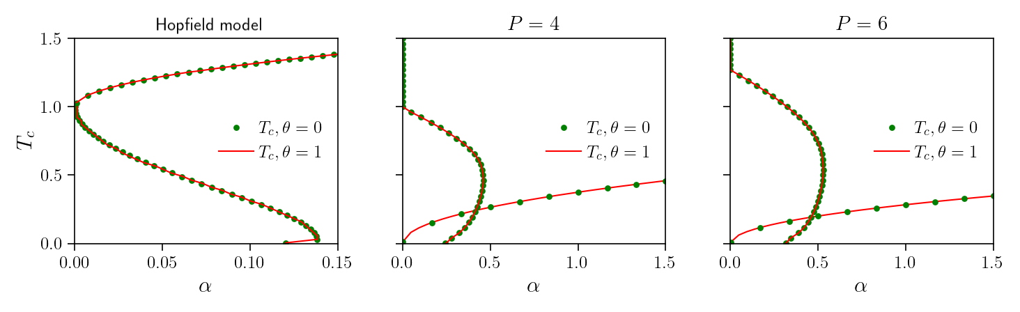
Figure 5: RS instability lines for the Hopfield model (left) and Hebbian networks with $P$-node interactions, with $P=4$ (mid) and $P=6$ (right), obtained via our method for $\theta\to 0$ and $\theta\to 1$. In the all the case the lines obtained for $\theta\to 0$ and $\theta\to 1$ are indistinguishable.

B.2 Hebbian Networks with multi-node interactions

Here we apply the same analysis to Hebbian networks with multi-node interactions, defined by the Hamiltonian given in Eq. (35). Our objective is to prove that the 1RSB quenched free-energy is smaller than its replica symmetric counterpart i.e. $f_{1RSB}(\beta^{{}^{\prime}},\alpha,\theta)<f_{RS}(\beta^{{}^{\prime}},\alpha)$ above a critical value of the effective parameter $\sqrt{\alpha}\beta^{\prime}$. To this purpose we expand, to linear orders in $\theta$, the 1RSB quenched free-energy around $\theta=0$, as shown in (94). Since the self-consistency equations also depend on $\theta$, we need to expand them too. Following the same steps as in the Hopfield model, we can write ${\bar{m}_{1}}$ as in (100), with $C({\color[rgb]{0,0,0}{\bar{m}},\,}\bar{q},\tilde{q}_{0}({\bar{m}},\bar{q}))$ as in (128), $\bar{q}_{1}$ as in (97), with $A({\color[rgb]{0,0,0}{\bar{m}},\,}\bar{q},\tilde{q}_{0}({\color[rgb]{0,0,0}{\bar{m}},\,}\bar{q}))$ given in (126), and $\bar{q}_{0}$ as given in (98), where $\tilde{q}_{0}({\color[rgb]{0,0,0}{\bar{m}},\,}\bar{q})$ is the solution of the self-consistency equation

$$\bar{q}_{0} =\mathbb{E}_{1}\left(\mathbb{E}_{2}\tanh g({\color[rgb]{0,0,0}{\bar{m}},\,}\bar{q},\bar{q}_{0})\right)^{2}$$ (107)

and $B({\color[rgb]{0,0,0}{\bar{m}},\,}\bar{q},\tilde{q}_{0}({\color[rgb]{0,0,0}{\bar{m}},\,}\bar{q}))$ is given in (127). With the above expressions in hand, we can now calculate the derivative of $f_{\rm 1RSB}$ w.r.t. $\theta$ when $\theta=0$, as needed in (94)

$$K({\color[rgb]{0,0,0}{\bar{m}},\,}\bar{q},\tilde{q}_{0}({\color[rgb]{0,0,0}{\bar{m}},\,}\bar{q})):=\partial_{\theta}(-\beta^{{}^{\prime}}f_{\rm 1RSB}({\color[rgb]{0,0,0}{\bar{m}_{1}},\,}\bar{q}_{1},\bar{q}_{0}|\theta))|_{\theta=0}$$

$$=\dfrac{-{\alpha\beta^{{}^{\prime}}}^{2}(P\!-\!1)}{4}(\bar{q}^{P}\!-\!({\tilde{q}_{0}}({\color[rgb]{0,0,0}{\bar{m}},\,}\bar{q}))^{P})\!+\!\dfrac{1}{2}\mathbb{E}_{1}\mathbb{E}_{2}\ln^{2}\cosh g({\color[rgb]{0,0,0}{\bar{m}},\,}\bar{q},\tilde{q}_{0}({\color[rgb]{0,0,0}{\bar{m}},\,}\bar{q}))-\dfrac{1}{2}\mathbb{E}_{1}\left(\mathbb{E}_{2}\ln\cosh g({\color[rgb]{0,0,0}{\bar{m}},\,}\bar{q},\tilde{q}_{0}({\color[rgb]{0,0,0}{\bar{m}},\,}\bar{q}))\right)^{2}$$ (108)

Again, we have that $K({\color[rgb]{0,0,0}{\bar{m}},\,}\bar{q},\bar{q})=0$, regardless of the value assigned to ${\bar{m}}$ (this follows from the fact that for $\theta=0$, $\bar{q}$ is an extremum of the free-energy). Next, we inspect the sign of $K({\color[rgb]{0,0,0}{\bar{m}},\,}\bar{q},\tilde{q}_{0}({\color[rgb]{0,0,0}{\bar{m}},\,}\bar{q}))$. To this purpose, we study $K({\color[rgb]{0,0,0}{\bar{m}},\,}\bar{q},x)$ for $x\in[0,\bar{q}]$ and locate its extrema, which are found from

$$\partial_{x}K({\color[rgb]{0,0,0}{\bar{m}},\,}\bar{q},x)= \dfrac{{\beta^{{}^{\prime}}}^{2}\alpha P(P-1)}{4}{x}^{P-2}\left[x-\mathbb{E}_{1}\left(\mathbb{E}_{2}\tanh g({\color[rgb]{0,0,0}{\bar{m}},\,}\bar{q},x)\right)^{2}\right]=0$$ (109)

as

$$x=\mathbb{E}_{1}\left(\mathbb{E}_{2}\tanh g({\color[rgb]{0,0,0}{\bar{m}},\,}\bar{q},x)\right)^{2}\equiv\tilde{q}_{0}({\color[rgb]{0,0,0}{\bar{m}},\,}\bar{q})$$ (110)

where the last equality follows from (107). Under the assumption that the extremum $x=\tilde{q}_{0}({\color[rgb]{0,0,0}{\bar{m}},\,}\bar{q})$ is global in the domain considered and reasoning as in the Hopfield case, we have that $K({\color[rgb]{0,0,0}{\bar{m}},\,}\bar{q},\tilde{q}_{0}({\color[rgb]{0,0,0}{\bar{m}},\,}\bar{q}))>0$ if $x=\tilde{q}_{0}({\color[rgb]{0,0,0}{\bar{m}},\,}\bar{q})$ is a maximum and $K({\color[rgb]{0,0,0}{\bar{m}},\,}\bar{q},\tilde{q}_{0}({\color[rgb]{0,0,0}{\bar{m}},\,}\bar{q}))<0$ if it is a minimum. In particular, if

$$\partial^{2}_{x}K({\color[rgb]{0,0,0}{\bar{m}},\,}\bar{q},x)|_{x=\tilde{q}_{0}({\color[rgb]{0,0,0}{\bar{m}},\,}\bar{q})}= -\dfrac{{\beta^{{}^{\prime}}}^{2}\alpha P(P-1)}{4}{\tilde{q}_{0}({\color[rgb]{0,0,0}{\bar{m}},\,}\bar{q})}^{P-2}$$

$$\cdot\left\{1-\dfrac{{\beta^{{}^{\prime}}}^{2}\alpha P(P-1){(\tilde{q}_{0}({\color[rgb]{0,0,0}{\bar{m}},\,}\bar{q}))}^{P-2}}{2}\mathbb{E}_{1}\left[\mathbb{E}_{2}\dfrac{1}{\cosh^{2}g({\color[rgb]{0,0,0}{\bar{m}},\,}\bar{q},\tilde{q}_{0}({\color[rgb]{0,0,0}{\bar{m}},\,}\bar{q}))}\right]^{2}\right\}$$ (111)

is negative, $K({\color[rgb]{0,0,0}{\bar{m}},\,}\bar{q},\tilde{q}_{0}({\color[rgb]{0,0,0}{\bar{m}},\,}\bar{q}))>0$ and $f_{1RSB}<f_{RS}$. This happens when the expression in the curly brackets of the equation above is negative, i.e. when the parameter $\alpha{\beta^{{}^{\prime}}}^{2}$ satisfies the inequality

$$\dfrac{\alpha{\beta^{{}^{\prime}}}^{2}P(P-1)(\tilde{q}_{0}({\color[rgb]{0,0,0}{\bar{m}},\,}\bar{q}))^{P-2}}{2}\mathbb{E}_{1}\left\{\mathbb{E}_{2}\left[\dfrac{1}{\cosh^{2}g({\color[rgb]{0,0,0}{\bar{m}},\,}\bar{q},\tilde{q}_{0}({\color[rgb]{0,0,0}{\bar{m}},\,}\bar{q}))}\right]\right\}^{2}>1.$$ (112)

The resulting critical line is found to be identical to the critical line (45) obtained from the expansion around $\theta=1$ (see Fig. 5, mid and right panels).

B.3 Spherical $P$-spin

Expanding for small $\theta$ the self-consistency equations (82), (83) to linear orders, we get

$$\dfrac{\beta^{2}}{2}P\bar{q}_{1}^{P-1} =\dfrac{\beta^{2}}{2}P\bar{q}_{0}^{P-1}+\dfrac{\bar{q}_{1}-\bar{q}_{0}}{(1-\bar{q}_{1})^{2}}+\theta A(\bar{q}_{0},\bar{q}_{1})$$ (113)

$$\dfrac{\beta^{2}}{2}P\bar{q}_{0}^{P-1} =\dfrac{\bar{q}_{0}}{(1-\bar{q}_{1})^{2}}+\theta B(\bar{q}_{0},\bar{q}_{1})$$ (114)

where the expression for $A(\bar{q}_{0},\bar{q}_{1})$ and $B(\bar{q}_{0},\bar{q}_{1})$ are provided in (135) and (136), respectively. If $\theta=0$, summing the two equations gives

$$\dfrac{\beta^{2}}{2}P\bar{q}_{1}^{P-1} =\dfrac{\bar{q}_{1}}{(1-\bar{q}_{1})^{2}}$$ (115)

showing that, to orders ${\mathcal{O}}(\theta^{0})$, $\bar{q}_{1}=\bar{q}$, while $\bar{q}_{0}$ fulfills the following self-consistency equation

$$\dfrac{\beta^{2}}{2}P\bar{q}_{0}^{P-1} =\dfrac{\bar{q}_{0}}{(1-\bar{q}_{1})^{2}}$$ (116)

whose solution is denoted with $\tilde{q}_{0}(\bar{q})$. The latter equation is solved by $\tilde{q}_{0}(\bar{q})=0$ (which corresponds to the paramagnetic solution and remains valid when ergodicity is broken, as explained earlier). Similarly, $\bar{q}_{1}=0$ is always a solution of (115), however the 1RSB scenario requires $\bar{q}_{1}>0$. As explained in the previous section, such non-zero solution appears at $T\leq T^{\star}=\sqrt{2(P-2)^{P-2}/P^{P-1}}$, which is below $T_{c}$ for any $P>2$, hence we can immediately conclude that the instability of the RS theory occurs at the larger temperature $T_{c}$, without further comparing the free-energies $1$RSB and RS for $\theta$ close to zero.

Appendix C Contributions to sub-leading orders

In this appendix we provide expressions for all the functions that we left unspecified in the main text, as they did not contribute to leading orders, including the functions $A(\bar{q}_{0},\bar{q}_{1})$ and $B(\bar{q}_{0},\bar{q}_{1})$ for all the models considered.

• For the Hopfield model, in the expansion around $\theta=1$ the subleading contributions to (22) and (24) are,

  $$A({\color[rgb]{0,0,0}{\bar{m}},\,}\bar{q}_{0},\bar{q}_{1})=2\mathbb{E}_{1} \left[\tanh\left(\beta{\bar{m}}+\dfrac{\beta z^{(1)}\sqrt{\alpha\bar{q}_{0}}}{(1-\beta(1-\bar{q}_{0})}\right)\right.$$

  $$\left.\cdot\dfrac{\mathbb{E}_{2}\log\cosh g_{1}({\color[rgb]{0,0,0}{\bar{m}},\,}\bar{q}_{0},\bar{q}_{1})\sinh g_{1}({\color[rgb]{0,0,0}{\bar{m}},\,}\bar{q}_{0},\bar{q}_{1})(1-\tanh g_{1}({\color[rgb]{0,0,0}{\bar{m}},\,}\bar{q}_{0},\bar{q}_{1}))}{\mathbb{E}_{2}\cosh g_{1}({\color[rgb]{0,0,0}{\bar{m}},\,}\bar{q}_{0},\bar{q}_{1})}\right],$$ (117)

  $$B({\color[rgb]{0,0,0}{\bar{m}},\,}\bar{q}_{0},\bar{q}_{1})=\dfrac{\beta^{3}\alpha(\bar{q}_{1}-\bar{q}_{0})}{(1-\beta(1-\bar{q}_{0}))^{2}}\left(\dfrac{\bar{q}_{0}}{(1-\beta(1-\bar{q}_{0}))}+\dfrac{(\bar{q}_{1}-\bar{q}_{0})}{(1-\beta(1-\bar{q}_{1}))}\right)$$

  $$\cdot\mathbb{E}_{1}\left\{1+\dfrac{\mathbb{E}_{2}\tanh^{2}g_{1}({\color[rgb]{0,0,0}{\bar{m}},\,}\bar{q}_{0},\bar{q}_{1})}{\mathbb{E}_{2}\cosh g_{1}({\color[rgb]{0,0,0}{\bar{m}},\,}\bar{q}_{0},\bar{q}_{1})}+\dfrac{\mathbb{E}_{2}\log\cosh g_{1}({\color[rgb]{0,0,0}{\bar{m}},\,}\bar{q}_{0},\bar{q}_{1})(1-\tanh^{2}g_{1}({\color[rgb]{0,0,0}{\bar{m}},\,}\bar{q}_{0},\bar{q}_{1}))}{\mathbb{E}_{2}\cosh g_{1}({\color[rgb]{0,0,0}{\bar{m}},\,}\bar{q}_{0},\bar{q}_{1})}\right\}$$

  $$-\dfrac{\beta^{3}\alpha(\bar{q}_{1}-\bar{q}_{0})^{2}}{(1-\beta(1-\bar{q}))^{3}}\mathbb{E}_{1}\left\{\tanh^{2}g_{1}({\color[rgb]{0,0,0}{\bar{m}},\,}\bar{q}_{0},\bar{q}_{1})\left(1-\right.\right.\left.\dfrac{\mathbb{E}_{2}\sinh g_{1}({\color[rgb]{0,0,0}{\bar{m}},\,}\bar{q}_{0},\bar{q}_{1})\tanh^{2}g_{1}({\color[rgb]{0,0,0}{\bar{m}},\,}\bar{q}_{0},\bar{q}_{1})}{\mathbb{E}_{2}\cosh g_{1}({\color[rgb]{0,0,0}{\bar{m}},\,}\bar{q}_{0},\bar{q}_{1})}\right)$$

  $$+\left(2-3\tanh^{3}\left(\beta{\bar{m}}+\dfrac{\beta z^{(1)}\sqrt{\alpha\bar{q}_{0}}}{(1-\beta(1-\bar{q}_{0})}\right)\right)\dfrac{\mathbb{E}_{2}\sinh g_{1}({\color[rgb]{0,0,0}{\bar{m}},\,}\bar{q}_{0},\bar{q}_{1})\tanh^{2}g_{1}({\color[rgb]{0,0,0}{\bar{m}},\,}\bar{q}_{0},\bar{q}_{1})}{\mathbb{E}_{2}\cosh g_{1}({\color[rgb]{0,0,0}{\bar{m}},\,}\bar{q}_{0},\bar{q}_{1})}$$

  $$\left.+\tanh\left(\beta{\bar{m}}+\dfrac{\beta z^{(1)}\sqrt{\alpha\bar{q}_{0}}}{(1-\beta(1-\bar{q}_{0})}\right)\dfrac{\mathbb{E}_{2}\log\cosh g_{1}({\color[rgb]{0,0,0}{\bar{m}},\,}\bar{q}_{0},\bar{q}_{1})\tanh g_{1}({\color[rgb]{0,0,0}{\bar{m}},\,}\bar{q}_{0},\bar{q}_{1})}{\mathbb{E}_{2}\cosh g_{1}({\color[rgb]{0,0,0}{\bar{m}},\,}\bar{q}_{0},\bar{q}_{1})}\right\}$$

  $$\dfrac{\beta^{3}\alpha(\bar{q}_{1}-\bar{q}_{0})^{2}}{2(1-\beta(1-\bar{q}_{0}))^{2}(1-\beta(1-\bar{q}_{1}))}\mathbb{E}_{1}\left\{\tanh\left(\beta{\bar{m}}+\dfrac{\beta z^{(1)}\sqrt{\alpha\bar{q}_{0}}}{(1-\beta(1-\bar{q}_{0})}\right)\right.$$

  $$\left.\cdot\dfrac{\mathbb{E}_{2}\sinh g_{1}({\color[rgb]{0,0,0}{\bar{m}},\,}\bar{q}_{0},\bar{q}_{1})\tanh g_{1}({\color[rgb]{0,0,0}{\bar{m}},\,}\bar{q}_{0},\bar{q}_{1})}{\mathbb{E}_{2}\cosh g_{1}({\color[rgb]{0,0,0}{\bar{m}},\,}\bar{q}_{0},\bar{q}_{1})}\right\}$$

  $$-\mathbb{E}_{1}\left\{\dfrac{\mathbb{E}_{2}\sinh g_{1}({\color[rgb]{0,0,0}{\bar{m}},\,}\bar{q}_{0},\bar{q}_{1})\tanh g_{1}({\color[rgb]{0,0,0}{\bar{m}},\,}\bar{q}_{0},\bar{q}_{1})\mathbb{E}_{2}\cosh g_{1}({\color[rgb]{0,0,0}{\bar{m}},\,}\bar{q}_{0},\bar{q}_{1})\log\cosh g_{1}({\color[rgb]{0,0,0}{\bar{m}},\,}\bar{q}_{0},\bar{q}_{1})}{(\mathbb{E}_{2}\cosh g_{1}({\color[rgb]{0,0,0}{\bar{m}},\,}\bar{q}_{0},\bar{q}_{1}))^{2}}\right\},$$ (118)

  and

  $$C({\color[rgb]{0,0,0}{\bar{m}},\,}\bar{q},\bar{q}_{1})=\left(-3\beta\dfrac{\sqrt{\alpha\bar{q}}}{\Delta_{1}(\bar{q})}-\beta\sqrt{\dfrac{\alpha(\bar{q}_{1}-\bar{q})}{\Delta_{1}(\bar{q})\Delta_{1}(\bar{q}_{1})}}\right)\mathbb{E}\tanh\left(\beta{\bar{m}}+\beta\sqrt{\dfrac{\alpha\bar{q}}{(1-\beta(1-\bar{q}))^{2}}}z\right)$$

  $$+2\beta\mathbb{E}\tanh^{3}\left(\beta{\bar{m}}+\beta\sqrt{\dfrac{\alpha\bar{q}}{(1-\beta(1-\bar{q}))^{2}}}z\right)\dfrac{\sqrt{\alpha\bar{q}}}{\Delta_{1}(\bar{q})}$$

  $$-\beta\dfrac{\sqrt{\alpha\bar{q}}}{\Delta_{1}(\bar{q})}\mathbb{E}_{1}\left[\sinh g_{1}({\bar{m}},\bar{q}_{0},\bar{q}_{1})\dfrac{\mathbb{E}_{2}\cosh g_{1}({\bar{m}},\bar{q}_{0},\bar{q}_{1})\tanh g_{1}({\bar{m}},\bar{q}_{0},\bar{q}_{1})\log\cosh g_{1}({\bar{m}},\bar{q}_{0},\bar{q}_{1})}{\mathbb{E}_{2}\cosh g_{1}({\bar{m}},\bar{q}_{0},\bar{q}_{1})}\right]$$

  $$+\left(\beta\dfrac{\sqrt{\alpha\bar{q}}}{\Delta_{1}(\bar{q})}+\beta\sqrt{\dfrac{\alpha(\bar{q}_{1}-\bar{q})}{\Delta_{1}(\bar{q})\Delta_{1}(\bar{q}_{1})}}\right)\left(\mathbb{E}_{1}\left[\dfrac{\mathbb{E}_{2}\cosh g_{1}({\bar{m}},\bar{q}_{0},\bar{q}_{1})\log\cosh g_{1}({\bar{m}},\bar{q}_{0},\bar{q}_{1})}{\mathbb{E}_{2}\cosh g_{1}({\bar{m}},\bar{q}_{0},\bar{q}_{1})}\right]\right.$$

  $$\left.+\mathbb{E}_{1}\left[\dfrac{2\cosh g_{1}({\bar{m}},\bar{q}_{0},\bar{q}_{1})\tanh^{2}g_{1}({\bar{m}},\bar{q}_{0},\bar{q}_{1})}{\mathbb{E}_{2}\cosh g_{1}({\bar{m}},\bar{q}_{0},\bar{q}_{1})}\right]\right)$$ (119)

  respectively, where $g_{1}({\color[rgb]{0,0,0}{\bar{m}},\,}\bar{q}_{0},\bar{q}_{1})$ is defined as in (18).

  For the expansion around $\theta=0$ the subleading contributions to (96) and (98) are

  $$A({\color[rgb]{0,0,0}{\bar{m}},\,}\bar{q}_{0},\bar{q}_{1})= \mathbb{E}_{1}\left[\mathbb{E}_{2}\tanh^{2}g_{0}({\color[rgb]{0,0,0}{\bar{m}},\,}\bar{q}_{1},\bar{q}_{0})\ln\cosh g_{0}({\color[rgb]{0,0,0}{\bar{m}},\,}\bar{q}_{1},\bar{q}_{0})\right]$$

  $$-\mathbb{E}_{1}\left[\mathbb{E}_{2}\tanh^{2}\mathbb{E}_{2}\ln\cosh g_{0}({\color[rgb]{0,0,0}{\bar{m}},\,}\bar{q}_{1},\bar{q}_{0})\right]$$

  $$+\dfrac{\beta^{3}\alpha\bar{q}_{1}(\bar{q}_{1}-\bar{q}_{0})}{\Delta_{1}(\bar{q}_{1})^{3}}\left[1-\mathbb{E}_{1}\left(\mathbb{E}_{2}\tanh^{2}g_{0}({\color[rgb]{0,0,0}{\bar{m}},\,}\bar{q}_{1},\bar{q}_{0})\right)\right]$$

  $$+\dfrac{3\beta^{3}\alpha(\bar{q}_{1}^{2}-\bar{q}_{0}^{2})}{\Delta_{1}(\bar{q}_{1})^{3}}\mathbb{E}_{1}\left[\mathbb{E}_{2}\tanh^{2}g_{0}({\color[rgb]{0,0,0}{\bar{m}},\,}\bar{q}_{1},\bar{q}_{2})\left(1-\tanh^{2}g_{0}({\color[rgb]{0,0,0}{\bar{m}},\,}\bar{q}_{1},\bar{q}_{0})\right)\right]$$ (120)

  $$B({\color[rgb]{0,0,0}{\bar{m}},\,}\bar{q}_{0},\bar{q}_{1})=2\Big{\{}\mathbb{E}_{1}\left[\mathbb{E}_{2}\tanh g_{0}({\color[rgb]{0,0,0}{\bar{m}},\,}\bar{q}_{1},\bar{q}_{0})\mathbb{E}_{2}\log\cosh g_{0}({\color[rgb]{0,0,0}{\bar{m}},\,}\bar{q}_{1},\bar{q}_{0})\tanh g_{0}({\color[rgb]{0,0,0}{\bar{m}},\,}\bar{q}_{1},\bar{q}_{0})\right]$$

  $$-\mathbb{E}_{1}\left[\mathbb{E}_{2}\log\cosh g_{0}({\color[rgb]{0,0,0}{\bar{m}},\,}\bar{q}_{1},\bar{q}_{0})\left(\mathbb{E}_{2}\tanh g_{0}({\color[rgb]{0,0,0}{\bar{m}},\,}\bar{q}_{1},\bar{q}_{0})\right)^{2}\right]$$

  $$+\dfrac{2\beta^{2}\alpha\bar{q}_{0}(\bar{q}_{1}-\bar{q}_{0})}{\Delta_{1}(\bar{q}_{1})^{3}}\mathbb{E}_{1}\left[\mathbb{E}_{2}\left(1-\tanh^{2}g_{0}({\color[rgb]{0,0,0}{\bar{m}},\,}\bar{q}_{1},\bar{q}_{0})\right)\right]$$

  $$-\dfrac{4\beta^{3}\alpha\bar{q}_{0}(\bar{q}_{1}-\bar{q}_{0})}{\Delta_{1}(\bar{q}_{1})^{3}}\mathbb{E}_{1}\left[\mathbb{E}_{2}\tanh g_{0}({\color[rgb]{0,0,0}{\bar{m}},\,}\bar{q}_{1},\bar{q}_{0})(1-\tanh^{2}g_{0}({\color[rgb]{0,0,0}{\bar{m}},\,}\bar{q}_{1},\bar{q}_{0}))\mathbb{E}_{2}\tanh^{2}g_{0}(\bar{q}_{1},\bar{q}_{0})\right]$$

  $$+\dfrac{2\beta^{3}\alpha\bar{q}_{0}(\bar{q}_{1}-\bar{q}_{0})}{\Delta_{1}(\bar{q}_{1})^{3}}\mathbb{E}_{1}\left[\mathbb{E}_{2}\tanh^{2}g_{0}({\color[rgb]{0,0,0}{\bar{m}},\,}\bar{q}_{1},\bar{q}_{0})\mathbb{E}_{2}\left(1-\tanh^{2}g_{0}({\color[rgb]{0,0,0}{\bar{m}},\,}\bar{q}_{1},\bar{q}_{0})\right)\right]$$

  $$+\dfrac{\beta^{2}\alpha(\bar{q}_{1}-\bar{q}_{0})^{2}}{\Delta_{1}(\bar{q}_{1})^{3}}\mathbb{E}_{1}\left[\mathbb{E}_{2}\tanh g_{0}({\color[rgb]{0,0,0}{\bar{m}},\,}\bar{q}_{1},\bar{q}_{0})\mathbb{E}_{2}\tanh g_{0}({\color[rgb]{0,0,0}{\bar{m}},\,}\bar{q}_{1},\bar{q}_{0})(1-\tanh^{2}g_{0}({\color[rgb]{0,0,0}{\bar{m}},\,}\bar{q}_{1},\bar{q}_{0}))\right]\Big{\}}$$ (121)

  and

  $$C({\color[rgb]{0,0,0}{\bar{m}},\,}\bar{q},\bar{q}_{0})= \dfrac{\alpha\beta^{3}\bar{q}_{1}(\bar{q}_{1}-\bar{q}_{0})}{(1-\beta(1-\bar{q}_{1}))^{3}}\mathbb{E}\left[\left(1-\tanh^{2}g_{0}({\color[rgb]{0,0,0}{\bar{m}},\,}\bar{q}_{1},\bar{q}_{0})\right)\log\cosh g_{0}({\color[rgb]{0,0,0}{\bar{m}},\,}\bar{q}_{1},\bar{q}_{0})\right.$$

  $$\left.+\tanh^{2}g_{0}({\color[rgb]{0,0,0}{\bar{m}},\,}\bar{q}_{1},\bar{q}_{0})-2\tanh g_{0}({\color[rgb]{0,0,0}{\bar{m}},\,}\bar{q}_{1},\bar{q}_{0})+2\tanh^{3}g_{0}({\color[rgb]{0,0,0}{\bar{m}},\,}\bar{q}_{1},\bar{q}_{0})\right]$$ (122)

  where $g_{0}({\color[rgb]{0,0,0}{\bar{m}},\,}\bar{q}_{0},\bar{q}_{1})$ is defined in (95).

• For Hebbian networks with $P$-node interactions, the subleading contributions to the overlaps $\bar{q}_{0}$ and $\bar{q}_{1}$ in the expansion around $\theta=1$ are given by

  $$A({\color[rgb]{0,0,0}{\bar{m}},\,}\bar{q}_{0},\bar{q}_{1})= 2\mathbb{E}_{1}\left\{\dfrac{\mathbb{E}_{2}\ln\cosh g({\color[rgb]{0,0,0}{\bar{m}},\,}\bar{q}_{1},\bar{q}_{0})\sinh g({\color[rgb]{0,0,0}{\bar{m}},\,}\bar{q}_{1},\bar{q}_{0})\tanh g({\color[rgb]{0,0,0}{\bar{m}},\,}\bar{q}_{1},\bar{q}_{0})}{\mathbb{E}_{2}\cosh g({\color[rgb]{0,0,0}{\bar{m}},\,}\bar{q}_{1},\bar{q}_{0})}\right\}-$$

  $$2\mathbb{E}_{1}\left\{\dfrac{\mathbb{E}_{2}\ln\cosh g({\color[rgb]{0,0,0}{\bar{m}},\,}\bar{q}_{1},\bar{q}_{0})\cosh g({\color[rgb]{0,0,0}{\bar{m}},\,}\bar{q}_{1},\bar{q}_{0})\mathbb{E}_{2}\sinh g({\color[rgb]{0,0,0}{\bar{m}},\,}\bar{q}_{1},\bar{q}_{0})\tanh g({\color[rgb]{0,0,0}{\bar{m}},\,}\bar{q}_{1},\bar{q}_{0})}{\left(\mathbb{E}_{2}\cosh g({\color[rgb]{0,0,0}{\bar{m}},\,}\bar{q}_{1},\bar{q}_{0})\right)^{2}}\right\},$$ (123)

  $$B({\color[rgb]{0,0,0}{\bar{m}},\,}\bar{q}_{0},\bar{q}_{1})= 2\mathbb{E}_{1}\left\{\dfrac{\mathbb{E}_{2}\sinh g({\color[rgb]{0,0,0}{\bar{m}},\,}\bar{q}_{1},\bar{q}_{0})\tanh g({\color[rgb]{0,0,0}{\bar{m}},\,}\bar{q}_{1},\bar{q}_{0})\mathbb{E}_{2}\cosh g({\color[rgb]{0,0,0}{\bar{m}},\,}\bar{q}_{1},\bar{q}_{0})\log\cosh g({\color[rgb]{0,0,0}{\bar{m}},\,}\bar{q}_{1},\bar{q}_{0})}{\left(\mathbb{E}_{2}\cosh g({\color[rgb]{0,0,0}{\bar{m}},\,}\bar{q}_{1},\bar{q}_{0})\right)^{2}}\right\}$$

  $$-2\mathbb{E}_{1}\left\{\dfrac{\left(\mathbb{E}_{2}\sinh g({\color[rgb]{0,0,0}{\bar{m}},\,}\bar{q}_{1},\bar{q}_{0})\tanh g({\color[rgb]{0,0,0}{\bar{m}},\,}\bar{q}_{1},\bar{q}_{0})\right)^{2}\mathbb{E}_{2}\sinh g({\color[rgb]{0,0,0}{\bar{m}},\,}\bar{q}_{1},\bar{q}_{0})\log\cosh g({\color[rgb]{0,0,0}{\bar{m}},\,}\bar{q}_{1},\bar{q}_{0})}{\left(\mathbb{E}_{2}\cosh g({\color[rgb]{0,0,0}{\bar{m}},\,}\bar{q}_{1},\bar{q}_{0})\right)^{3}}\right\},$$ (124)

  $$C({\color[rgb]{0,0,0}{\bar{m}},\,}\bar{q}_{0},\bar{q}_{1})= \mathbb{E}_{1}\left[\dfrac{\mathbb{E}_{2}\sinh g({\color[rgb]{0,0,0}{\bar{m}},\,}\bar{q}_{1},\bar{q}_{0})\log\cosh g({\color[rgb]{0,0,0}{\bar{m}},\,}\bar{q}_{1},\bar{q}_{0})}{\mathbb{E}_{2}\cosh g({\color[rgb]{0,0,0}{\bar{m}},\,}\bar{q}_{1},\bar{q}_{0})}\right]-$$

  $$\mathbb{E}_{1}\left[\dfrac{\mathbb{E}_{2}\sinh g({\color[rgb]{0,0,0}{\bar{m}},\,}\bar{q}_{1},\bar{q}_{0})\mathbb{E}_{2}\cosh g({\color[rgb]{0,0,0}{\bar{m}},\,}\bar{q}_{1},\bar{q}_{0})\log\cosh g({\color[rgb]{0,0,0}{\bar{m}},\,}\bar{q}_{1},\bar{q}_{0})}{\left(\mathbb{E}_{2}\cosh g({\color[rgb]{0,0,0}{\bar{m}},\,}\bar{q}_{1},\bar{q}_{0})\right)^{2}}\right]$$ (125)

  respectively, whereas, for the expansion around $\theta=0$ they evaluate to

  $$A({\color[rgb]{0,0,0}{\bar{m}},\,}\bar{q}_{0},\bar{q}_{1})= \mathbb{E}_{1}\mathbb{E}_{2}\ln\cosh g({\color[rgb]{0,0,0}{\bar{m}},\,}\bar{q}_{1},\bar{q}_{0})\tanh^{2}g({\color[rgb]{0,0,0}{\bar{m}},\,}\bar{q}_{1},\bar{q}_{0})$$

  $$-\mathbb{E}_{1}\left(\mathbb{E}_{2}\ln\cosh g({\color[rgb]{0,0,0}{\bar{m}},\,}\bar{q}_{1},\bar{q}_{0})\mathbb{E}_{2}\tanh^{2}g({\color[rgb]{0,0,0}{\bar{m}},\,}\bar{q}_{1},\bar{q}_{0})\right)$$ (126)

  $$B({\color[rgb]{0,0,0}{\bar{m}},\,}\bar{q}_{0},\bar{q}_{1})= \left\{2\mathbb{E}_{1}\left[\mathbb{E}_{2}\tanh g({\color[rgb]{0,0,0}{\bar{m}},\,}\bar{q}_{1},\bar{q}_{0})\mathbb{E}_{2}\ln\cosh g({\color[rgb]{0,0,0}{\bar{m}},\,}\bar{q}_{1},\bar{q}_{0})\tanh g({\color[rgb]{0,0,0}{\bar{m}},\,}\bar{q}_{1},\bar{q}_{0})\right]\right.$$

  $$\left.-2\mathbb{E}_{1}\left[\left(\mathbb{E}_{2}\tanh g({\color[rgb]{0,0,0}{\bar{m}},\,}\bar{q}_{1},\bar{q}_{0})\right)^{2}\mathbb{E}_{2}\ln\cosh g({\color[rgb]{0,0,0}{\bar{m}},\,}\bar{q}_{1},\bar{q}_{0})\right]\right\},$$ (127)

  $$C({\color[rgb]{0,0,0}{\bar{m}},\,}\bar{q}_{0},\bar{q}_{1})= \mathbb{E}_{1}\left[\mathbb{E}_{2}\tanh g({\color[rgb]{0,0,0}{\bar{m}},\,}\bar{q}_{1},\bar{q}_{0})\log\cosh g({\color[rgb]{0,0,0}{\bar{m}},\,}\bar{q}_{1},\bar{q}_{0})\right]$$

  $$-\mathbb{E}_{1}\left[\mathbb{E}_{2}\tanh g({\color[rgb]{0,0,0}{\bar{m}},\,}\bar{q}_{1},\bar{q}_{0})\mathbb{E}_{2}\log\cosh g({\color[rgb]{0,0,0}{\bar{m}},\,}\bar{q}_{1},\bar{q}_{0})\right]$$ (128)

  where $g({\color[rgb]{0,0,0}{\bar{m}},\,}\bar{q}_{1},\bar{q}_{0})$ is defined in (39).

• For the Sherrington-Kirkpatrick model the subleading contributions to the overlaps $\bar{q}_{0}$ and $\bar{q}_{1}$ in the expansion around $\theta=1$ are given by

  $$A(\bar{q}_{0},\bar{q}_{1})=\mathbb{E}_{1} \left\{\dfrac{\mathbb{E}_{2}\log\cosh g(\bar{q}_{0},\bar{q}_{1})\sinh g(\bar{q}_{0},\bar{q}_{1})\tanh g(\bar{q}_{0},\bar{q}_{1})\mathbb{E}_{2}\cosh g(\bar{q}_{0},\bar{q}_{1})}{(\mathbb{E}_{2}\cosh g)^{2}}\right.$$

  $$\left.-\dfrac{\mathbb{E}_{2}\sinh g(\bar{q}_{0},\bar{q}_{1})\tanh g(\bar{q}_{0},\bar{q}_{1})\mathbb{E}_{2}\cosh g(\bar{q}_{0},\bar{q}_{1})\log\cosh g(\bar{q}_{0},\bar{q}_{1})}{(\mathbb{E}_{2}\cosh g(\bar{q}_{0},\bar{q}_{1}))^{2}}\right\}$$ (129)

  $$B(\bar{q}_{0},\bar{q}_{1})= \mathbb{E}_{1}\left\{\dfrac{\mathbb{E}_{2}\log\cosh g(\bar{q}_{0},\bar{q}_{1})\sinh g(\bar{q}_{0},\bar{q}_{1})\mathbb{E}_{2}\cosh g(\bar{q}_{0},\bar{q}_{1})}{(\mathbb{E}_{2}\cosh g(\bar{q}_{0},\bar{q}_{1}))^{2}}\right.$$

  $$\left.-\dfrac{\mathbb{E}_{2}\sinh g(\bar{q}_{0},\bar{q}_{1})\mathbb{E}_{2}\cosh g(\bar{q}_{0},\bar{q}_{1})\log\cosh g(\bar{q}_{0},\bar{q}_{1})}{(\mathbb{E}_{2}\cosh g(\bar{q}_{0},\bar{q}_{1}))^{2}}\right\}.$$ (130)

  where $g(\bar{q}_{1},\bar{q}_{0})$ is defined in (50).

• For the Ising P-spin model, these terms, in the expansion around $\theta=1$, evaluate to

  $$A(\bar{q}_{0},\bar{q}_{1})= \mathbb{E}_{1}\left\{\dfrac{\mathbb{E}_{2}\log\cosh g(\bar{q}_{1},\bar{q}_{0})\sinh g(\bar{q}_{1},\bar{q}_{0})\tanh g(\bar{q}_{1},\bar{q}_{0})\mathbb{E}_{2}\cosh g(\bar{q}_{1},\bar{q}_{0})}{(\mathbb{E}_{2}\cosh g(\bar{q}_{1},\bar{q}_{0}))^{2}}\right.$$

  $$\left.-\dfrac{\mathbb{E}_{2}\sinh g(\bar{q}_{1},\bar{q}_{0})\tanh g(\bar{q}_{1},\bar{q}_{0})\mathbb{E}_{2}\cosh g(\bar{q}_{1},\bar{q}_{0})\log\cosh g(\bar{q}_{1},\bar{q}_{0})}{(\mathbb{E}_{2}\cosh g(\bar{q}_{1},\bar{q}_{0}))^{2}}\right\}$$ (131)

  $$B(\bar{q}_{0},\bar{q}_{1})= \mathbb{E}_{1}\left\{\dfrac{\mathbb{E}_{2}\log\cosh g(\bar{q}_{1},\bar{q}_{0})\sinh g(\bar{q}_{1},\bar{q}_{0})\mathbb{E}_{2}\cosh g(\bar{q}_{1},\bar{q}_{0})}{(\mathbb{E}_{2}\cosh g(\bar{q}_{1},\bar{q}_{0}))^{2}}\right.$$

  $$\left.-\dfrac{\mathbb{E}_{2}\sinh g(\bar{q}_{1},\bar{q}_{0})\mathbb{E}_{2}\cosh g(\bar{q}_{1},\bar{q}_{0})\log\cosh g(\bar{q}_{1},\bar{q}_{0})}{(\mathbb{E}_{2}\cosh g(\bar{q}_{1},\bar{q}_{0}))^{2}}\right\}.$$ (132)

  where $g(\bar{q}_{1},\bar{q}_{0})$ is defined in (66).

• Finally, for the spherical $P$-spin model, the contributions to linear orders in the expansion around $\theta=1$ (see (84) and (85)) are

  $$A(\bar{q}_{0},\bar{q}_{1})= \dfrac{2\bar{q}_{0}(\bar{q}_{0}-\bar{q}_{1})}{(1-\bar{q}_{0})^{3}}$$ (133)

  $$B(\bar{q}_{0},\bar{q}_{1})= \dfrac{(\bar{q}_{1}-\bar{q}_{0})^{2}}{(1-\bar{q}_{0})(1-\bar{q}_{1})}+\dfrac{2\bar{q}_{0}(\bar{q}_{0}-\bar{q}_{1})}{(1-\bar{q}_{0})^{3}}.$$ (134)

  while the contributions to linear orders in the expansion around $\theta=0$ (see (113) and (114)) are:

  $$A(\bar{q}_{0},\bar{q}_{1})= \dfrac{(\bar{q}_{1}^{2}-\bar{q}_{0}^{2})}{(1-\bar{q}_{1})^{3}}$$ (135)

  $$B(\bar{q}_{0},\bar{q}_{1})= \dfrac{2\bar{q}_{0}(\bar{q}_{1}-\bar{q}_{0})}{(1-\bar{q}_{1})^{3}}$$ (136)

References

• (1) E. Agliari, L. Albanese, A. Barra, and G. Ottaviani. Replica symmetry breaking in neural networks: A few steps toward rigorous results. Journal of Physics A: Mathematical and Theoretical, 53, 2020.
• (2) E. Agliari, F. Alemanno, A. Barra, M. Centonze, and A. Fachechi. Neural networks with a redundant representation: Detecting the undetectable. Physical Review Letters, 124:28301, 2020.
• (3) E. Agliari, F. Alemanno, A. Barra, and A. Fachechi. Generalized guerra’s interpolation schemes for dense associative neural networks. Neural Networks, 128:254–267, 2020.
• (4) L. Albanese, F. Alemanno, A. Alessandrelli, and A. Barra. Replica symmetry breaking in dense hebbian neural networks. Journal of Statistical Physics, 189(2):1–41, 2022.
• (5) D. J. Amit. Modeling brain function: The world of attractor neural networks. Cambridge university press, 1989.
• (6) A. Annibale, G. Gualdi, and A. Cavagna. Coexistence of supersymmetric and supersymmetry-breaking states in spherical spin-glasses. J. Phys. A: Math. Gen. 37 11311, 37(47):11311, 2004.
• (7) F. Antenucci, C. Conti, A. Crisanti, and L. Leuzzi. General phase diagram of multimodal ordered and disordered lasers in closed and open cavities. Phys. Rev. Lett., 114:043901, Jan 2015.
• (8) F. Antenucci, A. Crisanti, M. Ibáñez-Berganza, A. Marruzzo, and L. Leuzzi. Statistical mechanics models for multimode lasers and random lasers. Philosophical Magazine, 96(7-9):704–731, 2016.
• (9) F. Antenucci, A. Crisanti, and L. Leuzzi. Complex spherical 2 + 4 spin glass: A model for nonlinear optics in random media. Phys. Rev. A, 91:053816, May 2015.
• (10) F. Antenucci, M. Ibáñez Berganza, and L. Leuzzi. Statistical physics of nonlinear wave interaction. Phys. Rev. B, 92:014204, Jul 2015.
• (11) F. Antenucci, G. Lerario, B. S. Fernandéz, L. De Marco, M. De Giorgi, D. Ballarini, D. Sanvitto, and L. Leuzzi. Demonstration of self-starting nonlinear mode locking in random lasers. Phys. Rev. Lett., 126:173901, Apr 2021.
• (12) C. Baldassi, C. Borgs, J. T. Chayes, A. Ingrosso, C. Lucibello, L. Saglietti, and R. Zecchina. Unreasonable effectiveness of learning neural networks: From accessible states and robust ensembles to basic algorithmic schemes. Proceedings of the National Academy of Sciences, 113(48):E7655–E7662, 2016.
• (13) C. Baldassi, C. Lauditi, E. M. Malatesta, G. Perugini, and R. Zecchina. Unveiling the structure of wide flat minima in neural networks. Physical Review Letters, 127(27):278301, 2021.
• (14) X. Bardina, D. Márquez-Carreras, C. Rovira, and S. Tindel. The p-spin interaction model with external field. Potential Analysis, 21:311–362, 2004.
• (15) A. Barra, G. Genovese, F. Guerra, and D. Tantari. How glassy are neural networks? Journal of Statistical Mechanics: Theory and Experiment, 2012(07):P07009, 2012.
• (16) T. Castellani and A. Cavagna. Spin-glass theory for pedestrians. Journal of Statistical Mechanics: Theory and Experiment, 2005(05):P05012, 2005.
• (17) P. Charbonneau, Y. Hu, A. Raju, J. P. Sethna, and S. Yaida. Morphology of renormalization-group flow for the de almeida–thouless–gardner universality class. Physical Review E, 99(2):022132, 2019.
• (18) W.-K. Chen. On the almeida-thouless transition line in the sherrington-kirkpatrick model with centered gaussian external field. Electronic Communications in Probability, 26:1–9, 2021.
• (19) A. Coolen. Statistical mechanics of recurrent neural networks i—statics. In Handbook of biological physics, volume 4, pages 553–618. Elsevier, 2001.
• (20) A. C. C. Coolen, R. Kühn, and P. Sollich. Theory of neural information processing systems. OUP Oxford, 2005.
• (21) A. Crisanti, D. J. Amit, and H. Gutfreund. Saturation level of the hopfield model for neural network. Europhysics Letters (EPL), 2:337–341, 8 1986.
• (22) A. Crisanti and L. Leuzzi. Spherical $2+p$ spin-glass model: An exactly solvable model for glass to spin-glass transition. Phys. Rev. Lett., 93:217203, Nov 2004.
• (23) A. Crisanti and L. Leuzzi. Spherical $2+p$ spin-glass model: An analytically solvable model with a glass-to-glass transition. Phys. Rev. B, 73:014412, Jan 2006.
• (24) A. Crisanti and H. J. Sommers. The spherical p-spin interaction spin glass model: the statics. Zeitschrift für Physik B Condensed Matter, 87:341–354, 1992.
• (25) J. R. de Almeida and D. J. Thouless. Stability of the sherrington-kirkpatrick solution of a spin glass model. Journal of Physics A: Mathematical and General, 11(5):983, 1978.
• (26) G. Folena, S. Franz, and F. Ricci-Tersenghi. Rethinking mean-field glassy dynamics and its relation with the energy landscape: The surprising case of the spherical mixed p-spin model. Phys. Rev. X, 10:031045, Aug 2020.
• (27) E. Gardner. Spin glasses with p-spin interactions. Nuclear Physics B, 257:747–765, 1985.
• (28) E. Gardner. Multiconnected neural network models. Journal of Physics A: General Physics, 20, 1987.
• (29) F. Guerra. Broken replica symmetry bounds in the mean field spin glass model. Communications in Mathematical Physics, 233:1–12, 2003.
• (30) F. Guerra. The replica symmetric region in the sherrington-kirkpatrick mean field spin glass model. the almeida-thouless line. arXiv preprint cond-mat/0604674, 2006.
• (31) G. S. Hartnett, E. Parker, and E. Geist. Replica symmetry breaking in bipartite spin glasses and neural networks. Physical Review E, 98(2):022116, 2018.
• (32) J. Höller and N. Read. One-step replica-symmetry-breaking phase below the de almeida–thouless line in low-dimensional spin glasses. Physical Review E, 101(4):042114, 2020.
• (33) D. Krotov and J. J. Hopfield. Dense associative memory for pattern recognition. Advances in Neural Information Processing Systems, pages 1180–1188, 2016.
• (34) C. Manai and S. Warzel. The de almeida–thouless line in hierarchical quantum spin glasses. Journal of Statistical Physics, 186(1):1–32, 2022.
• (35) H. Nishimori. Statistical physics of spin glasses and information processing: an introduction. Number 111. Clarendon Press, 2001.
• (36) D. Sherrington and S. Kirkpatrick. Solvable model of a spin-glass. Physical review letters, 35(26):1792, 1975.
• (37) H. Steffan and R. Kühn. Replica symmetry breaking in attractor neural network models. Zeitschrift für Physik B Condensed Matter, 95, 1994.
• (38) M. Talagrand et al. Spin glasses: a challenge for mathematicians: cavity and mean field models, volume 46. Springer Science & Business Media, 2003.
• (39) T. Temesvári and I. Kondor. Field theory for the almeida-thouless transition. arXiv preprint arXiv:2212.01654, 2022.
• (40) D. J. Thouless. Spin-glass on a bethe lattice. Phys. Rev. Lett., 56:1082–1085, Mar 1986.
• (41) F. L. Toninelli. About the almeida-thouless transition line in the sherrington-kirkpatrick mean-field spin glass model. EPL (Europhysics Letters), 60(5):764, 2002.
• (42) T. Tonolo, J. Niedda, and G. Gradenigo. Marginal stability in the spherical spin glass: on the competition between disorder and non-linearity. In preparation.
• (43) Y. Zhao, J. Qiu, M. Xie, and H. Huang. Equivalence between belief propagation instability and transition to replica symmetry breaking in perceptron learning systems. Physical Review Research, 4(2):023023, 2022.