CP Asymmetry in $\tau\to K\pi\nu_{\tau}$ within Non-Minimal $SU(5)$

Abstract

Direct CP asymmetry in semi-leptonic $\tau$ decays is an intriguing hint for new physics beyond the standard model. We investigate the CP asymmetry in $\tau^{-}\to K_{S}^{0}\pi^{-}\nu_{\tau}$ and $\tau^{-}\to K^{-}\pi^{0}\nu_{\tau}$ decays in non-minimal SU(5) model, with 45-dimensional Higgs multiplet. We show that the associate color-triplet scalar is a natural example of a scalar leptoquark that mediates the transition $\tau\to s\bar{u}\nu_{\tau}$, and accounts for the 2.8 $\sigma$ discrepancy between the $A_{\rm CP}(\tau^{-}\to K_{S}^{0}\pi^{-}\nu_{\tau})$ experimental results and the SM expectation. Furthermore, it predicts a sizable $A_{\rm CP}(\tau^{-}\to K^{-}\pi^{0}\nu_{\tau})$, of order ${\cal O}(10^{-3})$, which can be accessible in current and near future experiments.

I Introduction

Semi-leptonic $\tau$ decays are very interesting venue for investigating Physics Beyond the Standard Model (BSM). The CP asymmetry of $\tau\to K^{0}_{S}\pi\nu_{\tau}$ is an example of an observation that points to new physics. The Belle collaboration reported evidence for CP violation in the $\tau\to K_{S}\pi\nu$ decay mode in 2011 [1], which the BaBar collaborations later confirmed [2]. It was the first time to observe CP violation in a purely leptonic decay process. The observation of direct CP violation in the $\tau\to K^{0}_{S}\pi\nu$ decay has sparked further research into physics BSM. According to the result reported by BaBar collaborations, the CP asymmetry in $\tau^{-}\to K_{S}^{0}\pi^{-}\nu_{\tau}$ decay is given by [2].

$$A_{\rm CP}(\tau^{+}\to K_{S}^{0}\pi^{+}\nu_{\tau}) = \frac{\Gamma(\tau^{+}\to K_{S}^{0}\pi^{+}\nu_{\tau})-\Gamma(\tau^{-}\to K_{S}^{0}\pi^{-}\nu_{\tau})}{\Gamma(\tau^{-}\to K_{S}^{0}\pi^{-}\nu_{\tau})-\Gamma(\tau^{+}\to K_{S}^{0}\pi^{+}\nu_{\tau})}$$ (1)

$$= -(3.6\pm 2.3\pm 1.1)\times 10^{-3}.$$

According to the Standard Model (SM) this process occurs via $\tau^{-}\to s\bar{u}\nu_{\tau}$ transition and no direct CP violation signal is expected. However due to the CP violation in $K^{0}-\bar{K}^{0}$ mixing at one loop level, the SM expectation of $A_{\rm CP}(\tau^{+}\to K_{S}^{0}\pi^{+}\nu_{\tau})$ is of order $2\times Re(\varepsilon_{K})$, and the total signal should be [3, 4, 5, 6]

$$A_{\rm CP}(\tau^{+}\to K_{S}^{0}\pi^{+}\nu_{\tau})|_{\rm SM}=(3.32\pm 0.06)\times 10^{-3}.$$ (2)

Therefore, there is a 2.8 sigma discrepancy that may indicate the presence of direct CP violation, which is absent in the SM. The presence of new sources of CP violation beyond the Cabibbo-Kobayashi-Maskawa (CKM) matrix in BSM can contribute to the $\tau\to K^{0}_{S}\pi\nu$ decay’s direct CP asymmetry. These contributions could result from new interactions involving particles not found in the standard model, such as charged Higgs boson, new particles in supersymmetric extensions of the SM or the scalar leptoquark.

The decay $\tau^{-}\to K^{-}\pi^{0}\nu_{\tau}$ has also been investigated experimentally, with a branching ratio of order $2.7\times 10^{-3}$ [7]. There have been attempts to measure the direct CP asymmetry of this decay, motivated by observations of CP violation in the $\tau^{-}\to K_{S}^{0}\pi^{-}\nu_{\tau}$ decay channel. However, no reported results have been provided so far. Because these two processes are correlated, we will predict the direct CP asymmetry in the $K^{-}$ channel associated with accounting for the $2.8$ discrepancy in $K_{S}^{0}$ channel, by the new physics CP violation effect.

Non-vanishing direct CP asymmetry requires an interference between two contributed amplitudes with non-vanishing weak and strong relative phases. If the total amplitude is given by $A_{1}e^{i\delta_{1}^{s}}e^{i\delta_{1}^{w}}+A_{2}e^{i\delta_{2}^{s}}e^{i\delta_{2}^{w}}$, then the CP asymmetry is given by

$$A_{\rm CP}=-4|A_{1}||A_{2}|\sin\delta^{s}\sin\delta^{w},$$ (3)

where $\delta^{s}=\delta_{1}^{s}-\delta_{2}^{s}$ and $\delta^{w}=\delta_{1}^{w}-\delta_{2}^{w}$. Both $K^{-}$ and $K_{S}^{0}$ channels occur on quark level in the SM via the tree level transition $\tau\to s\bar{u}\nu_{\tau}$, so their amplitudes are essentially real. After going beyond the tree level, the SM predicts negligibly direct CP asymmetry of order $10^{-12}$ [8]. Previous studies of CP violation in this decay channel has been conducted in supersymmetric extension of the SM [9, 10], multi Higgs models with complex couplings [11] and effective models with scalar leptoquarks [11]. These studies demonstrated that the estimated direct CP asymmetry is so small that further research is warranted.

The scalar leptoquark is one of the best candidates for mediating this decay at the tree level. It contributes to the amplitude with scalar and tensor operators that have non-vanishing strong and CP weak phases that differ from the SM CKM phase. Furthermore, leptoquark is naturally predicted in GUT extensions of the SM. One version of the $SU(5)$ GUT model includes $45$ (adjoint) Higgs fields [12]. This model is known as the ”non-minimal $SO(5)$. The adjoint Higgs field contributes to $SU(5)$ breaking down to the SM gauge group and provides a good fit to the observed particle masses and mixing angles, thereby resolving one major problem with the minimal $SU(5)$. The color-triplet scalar is one of the components of the $45$ Higgs, which can be as light as TeV if fine tuning similar to the well-known doublet-triplet splitting in GUT models is considered [13]. It is worth noting that because it has no coupling with quark-quark [14], this triplet does not contribute to proton decay.

In this paper, we consider the above-mentioned $SU(5)$ color- triplet scalar, which is a natural example of scalar leptoquark. This type of leptoquark differs from the general adhoc examples of leptoquarks discussed in the literature. As previously stated, it interacts in a specific way, so it does not contribute to proton decay but does contribute to $\tau\to s\bar{u}\nu$ decay. We emphasize that this contribution can account for the observed direct CP asymmetry in $\tau\to K\pi\nu$ decay.

The paper is structured as follows. Section 2 provides a brief overview of the CP Asymmetry in $\tau\to K\pi\nu$ decay within the SM and beyond. Section 3 is devoted to discussing the $SU(5)$ scalar leptoquark and its associated interactions, emphasizing that while it does not contribute to proton decay, it can play a significant role in the decays under consideration. The analysis of the new contribution of our scalar leptoquark to direct CP asymmetries of the decay modes $\tau^{-}\to K^{0}_{S}\pi^{-}\nu$ and $\tau^{-}\to K^{-}\pi^{0}\nu$ is discussed in section 4. Finally our conclusions and prospects are give in section 5.

II CP Asymmetry in $\tau\to K\pi\nu$ decay

The effective Hamiltonian of $|\Delta S|=1$ $\tau$ decays is given by

$${\mathcal{H}}_{eff}=-\frac{G_{F}}{\sqrt{2}}V^{\star}_{us}\sum_{i=V,A,S,P,T}C_{i}(\mu)\,Q_{i}(\mu),$$ (4)

where $V_{us}$ is the CKM mixing matrix element and $Q_{i}$ represent the four-fermion local operators at low energy scale $\mu\simeq m_{\tau}$ where

$$Q_{V} = \big{(}\bar{\nu}_{\tau}\gamma_{\mu}\tau\big{)}\big{(}\bar{s}\gamma^{\mu}u\big{)},~{}~{}~{}~{}~{}~{}~{}~{}~{}Q_{A}=\big{(}\bar{\nu}_{\tau}\gamma_{\mu}\gamma_{5}\tau\big{)}\big{(}\bar{s}\gamma^{\mu}u\big{)},$$

$$Q_{S} = \big{(}\bar{\nu}_{\tau}\tau\big{)}\big{(}\bar{s}u\big{)},~{}~{}~{}~{}~{}~{}~{}~{}~{}~{}~{}~{}~{}~{}~{}~{}Q_{P}=\big{(}\bar{\nu}_{\tau}\gamma_{5}\tau\big{)}\big{(}\bar{s}u\big{)},$$

$$Q_{T} = \big{(}\bar{\nu}_{\tau}\sigma_{\mu\nu}(1+\gamma_{5})\tau\big{)}\big{(}\bar{s}\sigma^{\mu\nu}u\big{)},$$ (5)

with $\sigma_{\mu\nu}=\frac{i}{2}[\gamma_{\mu},\gamma_{\nu}]$. The Wilson coefficients, $C_{i}$, corresponding to the operators $Q_{i}$ can be expressed as

$$C_{i}=C^{SM}_{i}+C^{NP}_{i},$$ (6)

where $C^{SM}_{i}$ and $C^{NP}_{i}$ represent SM and NP contributions to the Wilson coefficients respectively. The Wilson coefficients $C_{i}$ are typically expressed in terms of three independent coefficients: $C_{V}$ (dominated by SM contribution), $C_{S}$, and $C_{T}$. The matrix elements of the vector, scalar and tensor quark currents in the operators listed in Eq.(5) relevant to the process $\tau^{-}\to K^{-}\pi^{0}\nu_{\tau}$, can be expressed as:

$$\langle K^{-}\pi^{0}|\bar{s}\gamma^{\mu}u|0\rangle = \frac{1}{\sqrt{2}}\bigg{(}(p_{K}-p_{\pi})^{\mu}f_{+}(s)+(p_{K}+p_{\pi})^{\mu}f_{-}(s)\bigg{)},$$

$$\langle K^{-}\pi^{0}|\bar{s}u|0\rangle = \frac{(M_{K}^{2}-M_{\pi}^{2})}{\sqrt{2}(m_{s}-m_{u})}f_{0}(s)=\frac{\Delta^{2}_{K\pi}}{\sqrt{2}(m_{s}-m_{u})}f_{0}(s),$$

$$\langle K^{-}\pi^{0}|\bar{s}\sigma^{\mu\nu}u|0\rangle = \frac{i(p_{K}^{\mu}p_{\pi}^{\nu}-p_{K}^{\nu}p_{\pi}^{\mu})}{\sqrt{2}M_{K}}B_{T}(s).$$ (7)

The matrix elements of the decay $\tau^{-}\to K^{0}_{S}\pi^{-}\nu_{\tau}$, on the other hand, can be obtained by multiplying the right hand side of the corresponding ones in Eq.(7) by $\sqrt{2}$. As shown in Ref.[11], the differential decay width of $\tau^{-}\to K^{-}\pi^{0}\nu_{\tau}$ is given by

$$\frac{d\Gamma}{ds} = G_{F}^{2}|V_{us}|^{2}|C_{V}|^{2}S_{\rm EW}\frac{\lambda^{1/2}(s,M_{\pi}^{2},M_{K}^{2})(m_{\tau}^{2}-s)^{2}\Delta^{4}_{K\pi}}{1024\pi^{3}m_{\tau}s^{3}}$$ (8)

$$\times \bigg{[}\frac{(m_{\tau}^{2}+2s)\lambda(s,M_{\pi}^{2},M_{K}^{2})}{3m_{\tau}^{2}\Delta^{4}_{K\pi}}\bigg{(}|f_{+}(s)-T(s)|^{2}+\frac{2(m_{\tau}^{2}-s)^{2}}{9sm_{\tau}^{2}}|T(s)|^{2}\bigg{)}+|S(s)|^{2}\bigg{]},$$

where $\lambda(x,y,z)$ is given by $\lambda(x,y,z)=x^{2}+y^{2}+z^{2}-2xy-2xz-2yz$. Here $s$ is the invariant mass of the $\pi K$ system defined as $s=(p_{K}+p_{\pi})^{2}$, $S_{\rm EW}=1.0194$ accounts for the electroweak running down to $m_{\tau}$, and $\Delta^{2}_{K\pi}=M_{K}^{2}-M_{\pi}^{2}$. The quantities $S(s)$ and $T(s)$ are defined as

$$S(s) = f_{0}(s)\bigg{(}1+\frac{s\,C_{S}}{m_{\tau}(m_{s}-m_{u})\,C_{V}}\bigg{)},$$

$$T(s) = \frac{3s}{m_{\tau}^{2}+2s}\frac{m_{\tau}\,C_{T}}{M_{K}C_{V}}\,B_{T}(s).$$ (9)

It should be noted that the differential decay width of $\tau^{-}\to K^{0}_{S}\pi^{-}\nu_{\tau}$ is twice that one of $\tau^{-}\to K^{-}\pi^{0}\nu_{\tau}$ due to the difference in their form factors by a factor $\sqrt{2}$. The decay rates $\Gamma(\tau^{-}\to K_{S}^{0}\pi^{-}\nu_{\tau})$ and $\Gamma(\tau^{-}\to K^{-}\pi^{0}\nu_{\tau})$ can be obtained after integrating the differential decay widths with respect to the kinematic variable $s$. This allows us to have a prediction of the direct CP asymmetry of the given decay mode. In fact, as concluded in Refs.[15, 11], this asymmetry can be generated through the interference between the SM vector operator and new physics tensor operator, while the new physics scalar operator does not contribute to the asymmetry. After fixing the matrix elements and other involved parameters with their central values, one finds that [15, 11]

$$|A_{CP}(\tau^{-}\to K_{S}^{0}\pi^{-}\nu_{\tau})| \;< \sim\; 0.03\times|{\rm Im}(C_{T})|,$$

$$|A_{CP}(\tau^{-}\to K^{-}\pi^{0}\nu_{\tau})| \;< \sim\; 0.014\times|{\rm Im}(C_{T})|,$$ (10)

III $SU(5)$ Scalar Leptoquark and its Role in $\tau\to K_{S}\pi\nu$

As previously advocated, extending the Higgs sector of $SU(5)$ by $45_{H}$ helps to solve some of the problems that this simple example of GUT model faces [16, 17, 18, 19]. The $45_{H}$ transforms under the SM gauge as

$$45_{H}=(8,2)_{1/2}\oplus(1,2)_{1/2}\oplus(3,1)_{-1/3}\oplus(3,3)_{-1/3}\oplus(6^{*},1){-1/3}\oplus(3^{*},2)_{-7/6}\oplus(3^{*},1)_{4/3}.$$ (11)

It also satisfies the following constraints: $45^{\alpha\beta}_{\gamma}=-45^{\beta\alpha}_{\gamma}$ and $\sum_{\alpha}^{5}(45)^{\alpha\beta}_{\alpha}=0$. Through non-vanishing Vacuum Expectation Values (VEVs) of $5_{H}$ and $45_{H}$: $\langle 5_{H}\rangle=v_{5},\langle 45_{H}\rangle^{15}_{1}=\langle 45_{H}\rangle^{25}_{2}=\langle 45_{H}\rangle^{35}_{3}=v_{45},\langle 45_{H}\rangle^{45}_{4}=-3v_{45}$, the electroweak symmetry $SU(2)_{L}\times U(1)_{Y}$ is spontaneously broken into $U(1)_{em}$.

The $45_{H}$ scalar triplets are defined as:

$$(3^{*},2)^{ij}_{c\ -7/6}\equiv(45_{H})^{ij}_{c}\equiv\Phi^{ij}_{c},$$ (12)

$$(3^{*},1)^{ab}_{k\ 4/3}\equiv(45_{H})^{ab}_{k}\equiv\Phi^{ab}_{k},$$

$$[(3,1)^{ib}_{c}\oplus(3,3)^{ib}_{c}]_{-1/3}\equiv(45_{H})^{ib}_{c}\equiv\Phi^{ib}_{c}.$$

It has been emphasized [14] that while the scalar triplets $\Phi^{ab}_{k}$ and $\Phi^{ib}_{c}$ contribute to the proton decay and they must be superheavy, the scalar triplet $\Phi^{ij}_{c}$ does not. It has no interaction terms that would cause proton decay. By writing $\Phi^{ij}_{c}$ as $(\phi^{i}_{1},\phi^{i}_{2})^{T}$, one can demonstrate that the scalar triplet has the following peculiar interactions in the weak eignestate basis[14]:

$${\cal L}=2Y^{\prime 2}_{AB}e^{\prime T}_{A}Cu^{\prime c}_{Bi}\phi^{i1*}+4(Y^{\prime 4}_{AB}-Y^{\prime 4}_{BA})u^{\prime iT}_{A}Ce^{\prime c}_{B}\phi_{i1}-2Y^{\prime 2}_{AB}\nu^{\prime T}_{A}Cu^{\prime c}_{Bi}\phi^{i2*}+4(Y^{\prime 4}_{AB}-Y^{\prime 4}_{BA})d^{\prime iT}_{A}Ce^{\prime c}_{B}\phi_{i2}.~{}$$

Working in the basis in which the weak eignestate basis $(d^{\prime},u^{\prime},\nu^{\prime},e^{\prime})$ are related to the mass eignestate basis $(d,u,\nu,e)$ via the trnasformations $d^{\prime}_{A}\to V^{CKM}_{AB}d_{B},~{}~{}\nu^{\prime}_{A}\to V^{\rm PMNS}_{AB}\nu_{B},~{}~{}u^{\prime}_{A}\to u_{A},~{}~{}e^{\prime}_{A}\to e_{A},$ and defining $Y^{2}_{AB}=Y^{\prime 2}_{AB}$, $Y^{4}_{AB}\equiv(Y^{\prime 4}_{AB}-Y^{\prime 4}_{BA})$ results in the Lagrangians expressing the Yukawa couplings describing the SM fermions interactions with the scalar leptoquark $\phi_{i2}$ and $\phi_{i1}$

$$\mathcal{L}_{\phi_{i1}} = -2Y^{2}_{AB}\bar{u}_{Bi}P_{L}e_{A}\phi^{i1*}-4Y^{4}_{AB}\bar{e}_{B}P_{L}u_{A}\phi_{i1}\!-2Y^{2\,*}_{AB}\bar{e}_{A}P_{R}u_{Bi}\phi^{i1}-4Y^{4\,*}_{AB}\bar{u}_{A}P_{R}e_{B}\phi^{*}_{i1}\!,$$

$$\mathcal{L}_{\phi_{i2}} = 2Y^{2}_{AB}V_{AK}^{\rm PMNS}\bar{u}_{Bi}P_{L}\nu_{k}\phi^{i2*}-4Y^{4}_{DB}V^{\rm CKM}_{DK}\bar{e}_{B}P_{L}d_{K}\phi_{i2}\!+2Y^{2\,*}_{AB}V_{AK}^{\rm PMNS*}\bar{\nu}_{K}P_{R}u_{Bi}\phi^{i2}$$ (14)

$$- 4Y^{4*}_{DB}V^{\rm CKM*}_{DK}\bar{d}_{K}P_{R}e_{B}\phi^{*}_{i2}\!,$$

where $P_{R,L}=(1\pm\gamma^{5})/2$ and we have used $C^{T}=-C$ and $\bar{\Psi}=\Psi_{L}^{cT}$. Clearly from the previous equation that the scalar leptoquarks $\phi_{i1}$ and $\phi_{i2}$ have electric charges $-5/3$ and $-2/3$ respectively. As can be seen also from the Lagrangians in Eq.(14) that, $\tau^{-}\to s\bar{u}\nu_{\tau}$ transition relevant to our process can be generated by integrating out the scalar leptoquark $\phi_{i2}$ while neutron EDM receive contributions after integrating out the scalar leptoquark $\phi_{i1}$. This feature in this model allows us to avoid the strong constraints imposed by neutron EDM on the Yukawa couplings relevant to the transition $\tau^{-}\to s\bar{u}\nu_{\tau}$ as we will show in the following. It should be remarked that in the previous studies both neutron EDM and $\tau^{-}\to s\bar{u}\nu_{\tau}$ transition receive contributions from one leptoquark. As a result, in those studies, the strong constraint obtained from the neutron EDM suppresses considerably the leptoquark contributions to the $\tau^{-}\to s\bar{u}\nu_{\tau}$ transition,

Integrating out $\phi_{i1}$ yields tensor contributions to the neutron EDM, which can be expressed by the effective Lagrangian $\mathcal{L}^{\rm EDM}_{T}$

$$\mathcal{L}^{\rm EDM}_{T} \equiv C^{\rm EDM}_{T}(\bar{\tau}\sigma_{\mu\nu}P_{R}\tau)(\bar{u}\sigma^{\mu\nu}P_{R}u)+{\rm h.c.},$$ (15)

The renormalization group evolution [20] of the operator $(\bar{\tau}\sigma_{\mu\nu}R\tau)(\bar{u}\sigma^{\mu\nu}Ru)$ can produce via insertion an up-quark EDM $d_{u}(\mu)$ [15]

$$\mathcal{L}_{\rm D}=-\frac{i}{2}d_{u}(\mu)\bar{u}\sigma^{\mu\nu}\gamma_{5}uF_{\mu\nu}.$$ (16)

Upon solving the RG following  [21, 22, 23] we obtain

$$d_{u}(\mu) = \frac{em_{\tau}}{\pi^{2}}\,Im\,C^{\rm EDM}_{T}(\mu)\log\frac{\Lambda}{\mu}$$ (17)

$$\simeq 3.6\,{\rm Im}\,C^{\rm EDM}_{T}(\mu)\log\frac{\Lambda}{\mu}\times 10^{-15}\,e\,cm.$$

From the experimental current $90\%$ C.L. upper bound on neutron EDM: $d_{n}=g_{T}^{u}(\mu)d_{u}(\mu)<1.8\times 10^{-26}\,e\,{\rm cm}$ [24, 25, 26], one obtains a strong constraint on ${\rm Im}C^{\rm EDM}_{T}(\mu)$. Thus, for a value $\Lambda\raise 1.29167pt\hbox{$\;>$\kern-7.5pt\raise-4.73611pt\hbox{$\sim\;$}}100{\rm GeV}$ and using and the recent lattice result [27] $g_{T}^{u}(\mu=2{\rm GeV})=-0.204(11)(10)$, one finds the constraint

$$|{\rm Im}C^{\rm EDM}_{T}(\mu_{\tau})|\raise 1.29167pt\hbox{$\;<$\kern-7.5pt\raise-4.73611pt\hbox{$\sim\;$}}8.8\times 10^{-12},$$ (18)

which yields

$$\left|{\rm Im}(Y^{2\,*}_{31}Y^{4\,*}_{13})\right|\raise 1.29167pt\hbox{$\;<$\kern-7.5pt\raise-4.73611pt\hbox{$\sim\;$}}8.8\times\big{[}\frac{m_{\phi_{i1}}}{GeV}\big{]}^{2}\times 10^{-12}.$$ (19)

It should be noted that, the above constraint is based on the assumption that there are no other contributions to $d_{n}$ that can cancel the effect of $C^{\rm EDM}_{T}$. As can be seen from Eq.(19) that $\left|{\rm Im}(Y^{2\,*}_{31}Y^{4\,*}_{13})\right|\raise 1.29167pt\hbox{$\;<$\kern-7.5pt\raise-4.73611pt\hbox{$\sim\;$}}8.8\times 10^{-6}$, for leptoquark masses $m_{\phi_{i1}}\simeq{\cal O}(1)$ TeV. This result agrees with the bound obtained in Eq.(31) in Ref.[15].

Possible constraints on the parameter space of the model can be obtained from the new contributions to the $D-\bar{D}$ mixing. This can be done upon integrating out the scalar leptoquark $\phi_{i1}$ leading to the effective Lagrangian $\mathcal{L}^{D\bar{D}}_{T}$

$$\mathcal{L}^{D\bar{D}}_{T} \equiv C^{D\bar{D}}_{T}(\bar{\tau}\sigma_{\mu\nu}P_{R}\tau)(\bar{c}\sigma^{\mu\nu}P_{R}u)+{\rm h.c.},$$ (20)

The double insertion of the operator $(\bar{\tau}\sigma_{\mu\nu}P_{R}\tau)(\bar{c}\sigma^{\mu\nu}P_{R}u)$ results in tensorial contribution to the $D-\bar{D}$ mixing that is proportional to $C^{D\bar{D}}_{T}=\frac{1}{4m^{2}_{\phi_{i1}}}Y^{2\,*}_{31}Y^{4\,*}_{23}$. Consequently, for a given leptoquark mass $m_{\phi_{i1}}$, one can obtain a bound on the Yukaw product $Y^{2\,*}_{31}Y^{4\,*}_{23}$.

The transition $\tau\to s\bar{u}v_{\tau}$ generating the decay process $\tau\to K^{0}_{S}\pi^{-}(K^{-}\pi^{0})\nu_{\tau}$ can be obtained upon integrating the leptoquark $\phi_{i2}$. Doing so and after using Fierz identities, we find that

$$\mathcal{L}_{eff}=-\frac{4}{m^{2}_{\phi_{i2}}}Y^{2\,*}_{A1}Y^{4\,*}_{D3}V^{\rm CKM*}_{D2}V_{A3}^{\rm PMNS*}\bigg{[}(\bar{\nu}_{\tau}P_{R}\tau)(\bar{s}P_{R}u)+\frac{1}{4}(\bar{\nu}_{\tau}\sigma_{\mu\nu}P_{R}\tau)(\bar{s}\sigma^{\mu\nu}P_{R}u)\ +\ {\rm h.c.}\bigg{]}.$$ (21)

The Yukawa couplings $Y^{2}$ and $Y^{4}$ are generally complex. In this case, the Wilson coefficients $C_{i}$, corresponding to the operators $Q_{i}$ in Eq.(5)are given by

$$C_{V} = 0,\,\,\,\,\,\,\,\,\,\,\,\,\,\,\,\,\,\,C_{S}=\frac{2\sqrt{2}\,Y^{2\,*}_{A1}Y^{4\,*}_{D3}V^{\rm CKM*}_{D2}V_{A3}^{\rm PMNS*}}{\,G_{F}V^{*}_{us}\,m^{2}_{\phi_{i2}}},\,\,\,\,\,\,\,\,\,\,\,\,\,\,\,\,\,\,C_{T}=\frac{1}{4}C_{S}.$$ (22)

Due to the strong constraint on $|Im(Y^{2\,*}_{31}Y^{4\,*}_{13})|$ obtained from the EDM of the neutron, we can neglect the contributions of $Y^{2\,*}_{31}Y^{4\,*}_{13}$ to ${\rm Im}(C_{T})$. This is the case also for the Yukawa product $Y^{2\,*}_{31}Y^{4\,*}_{23}$ which is expected to be suppressed by the constraint from $D-\bar{D}$ mixing as can be seen from the expression of $C^{D\bar{D}}_{T}$ given before. On the other hand and in order to maximize the CP asymmetry, we need large values of $Im(C_{T})$. This can be achieved by choosing $A=2$ and $D=2$ in Eq.(22) which correspond to large values of $V_{23}^{\rm PMNS*}$ and $V^{\rm CKM*}_{22}$ respectively. As a result, the relevant parameter space to our processes includes the leptoquark $\phi_{i2}$ mass and the Yukawa couplings product $Y^{2}_{21}Y^{4}_{23}$.

IV Results and Implications

In this section, we discuss how our $SU(5)$ Leptoquark contributes to the CP asymmetry of $\tau^{-}\to K^{-}\pi^{0}\nu_{\tau}$ and $\tau^{-}\to K_{S}^{0}\pi^{-}\nu_{\tau}$. The CP asymmetries of these decay processes are given in terms of the ${\rm Im}(C_{T})$, as shown in Eq.(10). From the discrepancy between the $1\sigma$ measured value of $A_{\rm CP}(\tau^{-}\to K_{S}^{0}\pi^{-}\nu_{\tau})$ and the SM expectation, one finds that ${\rm Im}(C_{T})$ is constrained as follows:

$$-0.342\leq{\rm Im}[C_{T}(m_{\tau})]\leq-0.118.$$ (23)

Here, the tensor Wilson coefficient at scale $m_{\tau}$, $C_{T}(m_{\tau})$, is defined in terms of tensor Wilson coefficient at scale $m_{\phi_{i2}}$, $C_{T}(m_{\phi_{i2}})$, through the renormalization group equation which can be expressed as

$$C_{T}(m_{\tau})=R_{T}(m_{\tau},m_{\phi_{i2}})\,C_{T}(m_{\phi_{i2}})\,,$$ (24)

where the evolution function $R_{T}(m_{\tau},m_{\phi_{i2}})$ at the leading logarithmic approximation is given by [28]

$$R_{T}(m_{\tau},m_{\phi_{i2}})\equiv\bigg{[}\frac{\alpha_{s}(m_{b})}{\alpha_{s}(m_{\tau})}\bigg{]}^{\frac{\gamma_{T}}{2\beta_{0}^{(4)}}}\,\bigg{[}\frac{\alpha_{s}(m_{t})}{\alpha_{s}(m_{b})}\bigg{]}^{\frac{\gamma_{T}}{2\beta_{0}^{(5)}}}\,\bigg{[}\frac{\alpha_{s}(m_{\phi_{i2}})}{\alpha_{s}(m_{t})}\bigg{]}^{\frac{\gamma_{T}}{2\beta_{0}^{(6)}}}\,,$$ (25)

here $\beta_{0}^{(n_{f})}=11-2n_{f}/3$ represents the leading-order coefficient of the QCD beta function, $n_{f}$ is the number of active quark flavours, and $\gamma_{T}=8/3$ [29] stands for the leading-order anomalous dimensions of the tensor current.

With the parameter space selection, it is critical to check that the predicted result of the branching ratio of $\tau^{-}\to K^{-}\nu_{\tau}$ to ensure that it remains within the experimental limits. The experimental results for the branching ratio of $\tau^{-}\to K^{-}\nu_{\tau}$ is given as ${\cal B}_{\rm Exp.}=(6.96\pm 0.10)\times 10^{-3}$ [7]. The SM expectation for this branching ratio can be expressed as

$${{\cal B}_{SM}}\left[{{\tau^{-}}\to K^{-}\nu_{\tau}}\right]=\frac{{{m^{3}_{{\tau^{-}}}}}}{{16\pi}}G_{F}^{2}{\tau_{{\tau^{-}}}}f_{{K}}^{2}{\left|{V^{*}_{us}}\right|^{2}}{\left({1-\frac{{m_{K^{-}}^{2}}}{{m_{{\tau^{-}}}^{2}}}}\right)^{2}}\left(1+\delta^{K}_{RC}\right)\,,$$ (26)

where $\delta^{K}_{RC}$ accounts for the short and long distance electromagnetic radiative corrections. Using the mean life $\tau_{\tau^{-}}=(290.3\pm 0.5)\times 10^{-15}s$ [7], $\delta^{\tau K^{-}}_{EM}=2.04(62)\%$ [30] and the results of the latest global SM analysis reported by the UTfit collaboration $|V_{us}|=0.2251(8)$ [31], $f_{\pi}=92.3(1)$ MeV [7] and $f_{K}=1.198f_{\pi}$ [7]. Numerically it leads to ${\cal B}_{SM}\sim 3.57\times 10^{-3}$. The branching ratio is modified by a New Physics (NP) contribution, such as leptoquark contribution given in Eq.(21), as follows:

$${{\cal B}_{NP}}={\cal B}_{SM}\bigg{(}1+\left|\frac{{m_{K}^{2}}}{\left(m_{u}+m_{s}\right)m_{\tau^{-}}}C_{S}\right|^{2}\bigg{)}$$ (27)

In this regard, the Wilson coefficient $C_{S}=4C_{T}$ is constrained by

$$|C_{S}|\raise 1.29167pt\hbox{$\;<$\kern-7.5pt\raise-4.73611pt\hbox{$\sim\;$}}\frac{(m_{u}+m_{s})m_{\tau}}{m_{K}^{2}}\left(\frac{{\cal B}_{Exp}}{{\cal B}_{SM}}-1\right)^{\frac{1}{2}}\simeq 0.67.$$ (28)

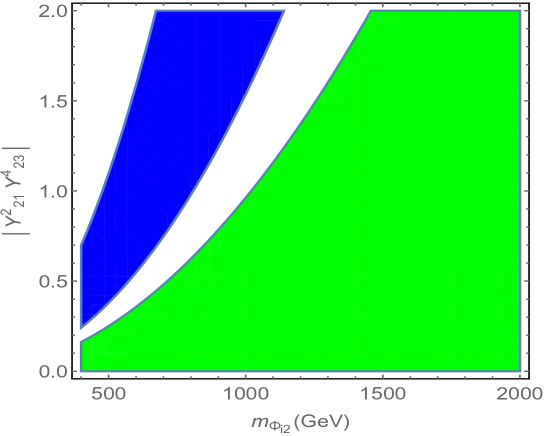
Figure 1: Allowed region of the parameter space $(m_{\phi_{i2}},|Y^{2}_{21}Y^{4}_{23}|)$ in blue (Green) color satisfying the obtained bound in Eq.(23) (Eq.28).

In Fig. 1, we plot in blue (Green) the allowed region of the parameter space $(m_{\phi_{i2}},|Y^{2}_{21}Y^{4}_{23}|)$ satisfying the obtained $1\sigma$ bound in Eq.(23) (Eq.28). As shown in the figure, there is no region in the $(m_{\phi_{i2}},|Y^{2}_{21}Y^{4}_{23}|)$ parameter space that meets both constraints. Therefore, the constraint from the branching ratio of of $\tau^{-}\to K^{-}\nu_{\tau}$ is stringent at $1\sigma$ level, and the new contributions of the scalar leptoquark cannot resolve the direct CP asymmetry of the decay $\tau^{-}\to K_{S}^{0}\pi^{-}\nu_{\tau}$. However, if we relax the limits in Eq.(23) to consider the $2\sigma$ level, we find that these new contributions can accommodate the mentioned CP asymmetry.

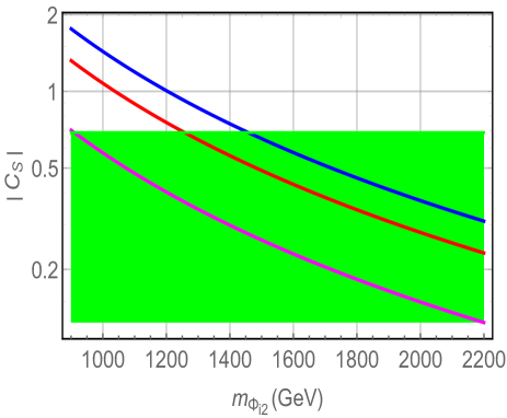
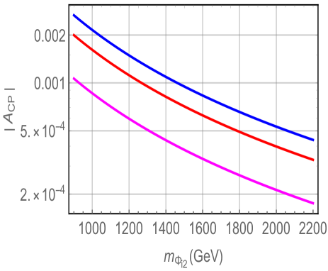
Figure 2: $|C_{S}|$ ($|A_{CP}|$) of the process $\tau^{-}\to K^{-}\pi^{0}\nu_{\tau}$ left (right) as function of leptoquark mass $|Y^{2}_{21}Y^{4}_{23}|=0.8,1.5,2.0$ in magenta, red and blue colors respectively. The green region represent the $1\sigma$ bound in eq.(28).

Our objective in this study is to give an estimation of the direct CP asymmetry of the decay mode $\tau^{-}\to K^{-}\pi^{0}\nu_{\tau}$. In Fig. 2, we show in the left plot $|C_{S}|$ at $m_{\tau}$ scale while in the right plot we display $|A_{CP}|$ of the mode $\tau^{-}\to K^{-}\pi^{0}\nu_{\tau}$ as a function of leptoquark mass at fixed Yukaw couplings product $|Y^{2}_{21}Y^{4}_{23}|=0.8,1.5,2.0$ in magenta, red and blue colors respectively. It should be noted that, the green region represent the $1\sigma$ bound in eq.(28). The left plot can be used to determine the value of the $|Y^{2}_{21}Y^{4}_{23}|$ corresponding to a given leptoquark mass, ensuring that the branching ratio of the decay $\tau^{-}\to K^{-}\nu_{\tau}$ remains consistent with its experimental value. From the right plot in Fig. 2, for these allowed values of parameter space $(m_{\phi_{i2}},|Y^{2}_{21}Y^{4}_{23}|)$, we can deduce from that $A_{\rm CP}(\tau\to K^{-}\pi\nu_{\tau})$ could be in the $10^{-3}$ to $10^{-4}$ range for a consistent branching ratio of $\tau^{-}\to K^{-}\nu_{\tau}$. This conclusion is supported by Fig.3, which shows the relationship between the $A_{\rm CP}(\tau\to K^{-}\pi\nu_{\tau})$ and ${\rm BR}(\tau\to K^{-}\nu_{\tau})$.

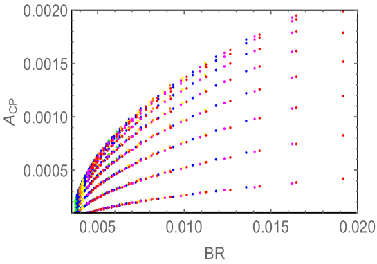
Figure 3: Correlation of $BR={{\cal B}_{NP}}\left[{{\tau^{-}}\to K^{-}\nu_{\tau}}\right]$ and $|A_{\rm CP}(\tau\to K^{-}\pi\nu_{\tau})|$ channel.

V Conclusion

In this paper, we have investigated the possibility of resolving the $2.8~{}\sigma$ deviation between the SM prediction and the experimental result of the CP asymmetry in the decay $\tau^{-}\to K_{S}^{0}\pi^{-}\nu_{\tau}$, using a low scale non-minimal $SU(5)$ mode. We emphasized that the non-minimal SU(5), in which the Higgs sector is extended by an extra 45-dimensional multiplet, provides a TeV scalar triplet leptoquark that generates direct CP asymmetry in semi-leptonic $\tau$ decay $\tau^{-}\to K_{S}^{0}\pi^{-}\nu_{\tau}$, and thus can account for this discrepancy. Furthermore, we demonstrated that, within the same parameter space, the CP asymmetry of $\tau^{-}\to K^{-}\pi^{0}\nu_{\tau}$ is of order ${\cal O}(10^{-3})$, which is a few orders of magnitude larger than the results obtained in other models beyond the SM. This can be attributed to the presence of Yukawa couplings of our leptoquark that do not contribute to proton decay, EDM and $D-\bar{D}$ mixing, enabling us to avoid the related constraints. The phases of these couplings allow us to enhance the CP asymmetries considerably. We also demonstrated that the branching ratio of $\tau\to K^{-}\nu_{\tau}$, after including the leptoquark contributions with large Yukawa couplings required to enhance the CP asymmetry $A_{\rm CP}(\tau\to K_{S}^{0}\pi^{-}\nu_{\tau})$, is well within the experimental limits.

References

• [1] M. Bischofberger et al. [Belle], Phys. Rev. Lett. 107, 131801 (2011) doi:10.1103/PhysRevLett.107.131801 [arXiv:1101.0349 [hep-ex]].
• [2] J. P. Lees et al. [BaBar], Phys. Rev. D 85, 031102 (2012) [erratum: Phys. Rev. D 85, 099904 (2012)] doi:10.1103/PhysRevD.85.031102 [arXiv:1109.1527 [hep-ex]].
• [3] Y. Grossman and Y. Nir, CP Violation in $\tau\to\nu\pi K_{S}$ and $D\to\pi K_{S}$: The Importance of $K_{S}-K_{L}$ Interference, JHEP 1204, 002 (2012) [arXiv:1110.3790 [hep-ph]].
• [4] I. I. Bigi and A. I. Sanda, A ‘known’ CP asymmetry in $\tau$ decays, Phys. Lett. B 625, 47 (2005) [arXiv:hep-ph/0506037].
• [5] G. Calderon, D. Delepine and G. L. Castro, Is there a paradox in CP asymmetries of $tau^{\pm}\to K_{[}L,\ S]\pi^{\pm}\nu$ decays?, Phys. Rev. D 75, 076001 (2007) [hep-ph/0702282 [HEP-PH]].
• [6] F. Z. Chen, X. Q. Li, Y. D. Yang and X. Zhang, Phys. Rev. D 100, no.11, 113006 (2019) doi:10.1103/PhysRevD.100.113006 [arXiv:1909.05543 [hep-ph]].
• [7] R. L. Workman et al. [Particle Data Group], PTEP 2022, 083C01 (2022) doi:10.1093/ptep/ptac097
• [8] D. Delepine, G. Lopez Castro and L. T. Lopez Lozano, Phys. Rev. D 72, 033009 (2005).
• [9] D. Delepine, G. Faisl, S. Khalil and G. L. Castro, Phys. Rev. D 74, 056004 (2006) doi:10.1103/PhysRevD.74.056004 [hep-ph/0608008].
• [10] D. Delepine, G. Faisel and S. Khalil, Phys. Rev. D 77, 016003 (2008) doi:10.1103/PhysRevD.77.016003 [arXiv:0710.1441 [hep-ph]].
• [11] D. Delepine, G. Faisel and C. A. Ramirez, Eur. Phys. J. C 81, no.4, 368 (2021) doi:10.1140/epjc/s10052-021-09150-4 [arXiv:1806.05090 [hep-ph]].
• [12] H. Georgi and S. L. Glashow, Phys. Rev. Lett. 32, 438–441, 1974.
• [13] S. Khalil and S. Salem, Nucl. Phys. B 876, 2013, hep-ph:1304.3689.
• [14] Ilja Dorsner, Svjetlana Fajfer, Nejc Kosnik, Phys. Rev. D 86, no. 1, 015013 (2012) [ arXiv:1204.0674v2 [hep-ph]].
• [15] V. Cirigliano, A. Crivellin and M. Hoferichter, Phys. Rev. Lett. 120, no.14, 141803 (2018) doi:10.1103/PhysRevLett.120.141803 [arXiv:1712.06595 [hep-ph]]. section III references
• [16] I. Dorsner and P. Fileviez Perez, Phys. Lett. B 642, 248-252 (2006) doi:10.1016/j.physletb.2006.09.034 [arXiv:hep-ph/0606062 [hep-ph]].
• [17] P. Fileviez Perez, [arXiv:0710.1321 [hep-ph]].
• [18] S. Khalil, S. Salem and M. Allam, Phys. Rev. D 89, 095011 (2014) [erratum: Phys. Rev. D 91, 119908 (2015)] doi:10.1103/PhysRevD.89.095011 [arXiv:1401.1482 [hep-ph]].
• [19] A. Ismael and S. Khalil, [arXiv:2301.02226 [hep-ph]].
• [20] E. E. Jenkins, A. V. Manohar and M. Trott, JHEP 01, 035 (2014) doi:10.1007/JHEP01(2014)035 [arXiv:1310.4838 [hep-ph]].
• [21] S. Bellucci, M. Lusignoli and L. Maiani, Nucl. Phys. B 189, 329-346 (1981) doi:10.1016/0550-3213(81)90384-9
• [22] G. Buchalla, A. J. Buras and M. K. Harlander, Nucl. Phys. B 337, 313-362 (1990) doi:10.1016/0550-3213(90)90275-I
• [23] V. Cirigliano, S. Davidson and Y. Kuno, Phys. Lett. B 771, 242-246 (2017) doi:10.1016/j.physletb.2017.05.053 [arXiv:1703.02057 [hep-ph]].
• [24] C. A. Baker, D. D. Doyle, P. Geltenbort, K. Green, M. G. D. van der Grinten, P. G. Harris, P. Iaydjiev, S. N. Ivanov, D. J. R. May and J. M. Pendlebury, et al. Phys. Rev. Lett. 97, 131801 (2006) doi:10.1103/PhysRevLett.97.131801 [arXiv:hep-ex/0602020 [hep-ex]].
• [25] J. M. Pendlebury, S. Afach, N. J. Ayres, C. A. Baker, G. Ban, G. Bison, K. Bodek, M. Burghoff, P. Geltenbort and K. Green, et al. Phys. Rev. D 92, no.9, 092003 (2015) doi:10.1103/PhysRevD.92.092003 [arXiv:1509.04411 [hep-ex]].
• [26] C. Abel, S. Afach, N. J. Ayres, C. A. Baker, G. Ban, G. Bison, K. Bodek, V. Bondar, M. Burghoff and E. Chanel, et al. Phys. Rev. Lett. 124, no.8, 081803 (2020) doi:10.1103/PhysRevLett.124.081803 [arXiv:2001.11966 [hep-ex]].
• [27] T. Bhattacharya, V. Cirigliano, R. Gupta, H. W. Lin and B. Yoon, Phys. Rev. Lett. 115, no.21, 212002 (2015) doi:10.1103/PhysRevLett.115.212002 [arXiv:1506.04196 [hep-lat]].
• [28] I. Doršner, S. Fajfer, A. Greljo, J. F. Kamenik and N. Košnik, Phys. Rept. 641, 1-68 (2016) doi:10.1016/j.physrep.2016.06.001 [arXiv:1603.04993 [hep-ph]].
• [29] J. A. Gracey, Phys. Lett. B 488, 175-181 (2000) doi:10.1016/S0370-2693(00)00859-5 [arXiv:hep-ph/0007171 [hep-ph]]. [30]
• [30] V. Cirigliano, D. Díaz-Calderón, A. Falkowski, M. González-Alonso and A. Rodríguez-Sánchez, JHEP 04, 152 (2022) doi:10.1007/JHEP04(2022)152 [arXiv:2112.02087 [hep-ph]].
• [31] M. Bona et al. [UTfit], [arXiv:2212.03894 [hep-ph]].