Improved self-consistency of the Reynolds stress tensor eigenspace perturbation for Uncertainty Quantification

Abstract

The limitations of turbulence closure models in the context of Reynolds-averaged Navier-Stokes (RANS) simulations play a significant part in contributing to the uncertainty of Computational Fluid Dynamics (CFD). Perturbing the spectral representation of the Reynolds stress tensor within physical limits is common practice in several commercial and open-source CFD solvers, in order to obtain estimates for the epistemic uncertainties of RANS turbulence models. Recent research revealed, that there is a need for moderating the amount of perturbed Reynolds stress tensor tensor to be considered due to upcoming stability issues of the solver. In this paper we point out that the consequent common implementation can lead to unintended states of the resulting perturbed Reynolds stress tensor. The combination of eigenvector perturbation and moderation factor may actually result in moderated eigenvalues, which are not linearly dependent on the originally unperturbed and fully perturbed eigenvalues anymore. Hence, the computational implementation is no longer in accordance with the conceptual idea of the Eigenspace Perturbation Framework. We verify the implementation of the conceptual description with respect to its self-consistency. Adequately representing the basic concept results in formulating a computational implementation to improve self-consistency of the Reynolds stress tensor perturbation.

I Introduction

Industrial aerodynamic designs increasingly rely on numerical analysis based on flow simulations using CFDhastargettrueComputational Fluid Dynamics (CFD) software. Such industrial applications usually feature turbulent flows. Due to its cost- and time-effective solution procedure, Reynolds-averaged Navier-Stokes (RANS) equations are an appropriate approach for design optimizations and virtual certification. Unfortunately, the RANShastargettrueReynolds-averaged Navier-Stokes (RANS) equations are not closed and, hence, require the determination of the second-moment Reynolds stress tensor. In this context, the Reynolds stress tensor is approximated using turbulence models. These models make assumptions regarding the relationship between the Reynolds stresses and available mean flow quantities, such as the mean velocity gradients, which limit their applicability in terms of accuracy on the one hand. On the other hand, the assumptions made in the formulation of closure models inevitably lead to uncertainties as soon as their range of validity is left. The quantification of these model-form uncertainties for industrial purposes is a demanding task in general.
Several approaches seek to account for these uncertainties at different modeling levels Duraisamy; XIAO20191. We focus on the EPFhastargettrueEigenspace Perturbation Framework (EPF) Emory; Iaccarino, which estimates the predictive uncertainty due to limitations in the turbulence model structure, namely its epistemic uncertainty. The EPFhastargettrueEPF is purely physics-based and introduces a series of perturbations to the shape, alignment and size of the modeled Reynolds stress ellipsoid to estimate its uncertainty. Because of its straight forward implementation, the EPFhastargettrueEPF has been used in diverse areas of application such as mechanical engineering razaaly2019optimization, aerospace engineering mishra2017uncertainty; cook2019optimization; mishra2020design; Chu2022a; Chu2022, civil engineering garcia2014quantifying; Lamberti, wind farm design EidiDataFree; Hornshoj, etc. The EPFhastargettrueEPF is the foundation of recent confidence-based design under uncertainty approaches gori2022confidence. There have been studies showing the potential to optimize it using data driven machine learning approaches Heyse; Eidi2022 and it has been applied for the virtual certification of aircraft designs Mukhopadhaya; nigam2021toolset. The EPFhastargettrueEPF has been integrated into several open and closed source flow solvers Edeling; Gorle2019; MishraSU2; MathaCF. This range of applications emphasizes the importance of the EPFhastargettrueEPF. Imperfections in the EPFhastargettrueEPF can have a cascading ramification to all these applications and fields.
There is need for VVhastargettrueVerification and Validation (V&V) for such novel methodologies. Validation focuses on the agreement of the computational simulation with physical reality oberkampf2002verification, which has been done for the EPFhastargettrueEPF in the aforementioned studies. On the other hand, verification focuses on the correctness of the programming and computational implementation of the conceptual model stern2001comprehensive. For the EPFhastargettrueEPF, this verification would involve the theory behind the conceptual model and the computational implementation. The theoretical foundations of the Reynolds stress tensor perturbations have been analyzed in detail mishra2019theoretical. In this investigation, we focus on the computational implementation of the EPFhastargettrueEPF, analyzing the consistency between the envisioned conceptual model and the actually implemented computational model.
In order to estimate the epistemic uncertainty for future design applications with respect to turbulence closure model, we review the current implementation of the framework in DLRhastargettrueDLR’s CFDhastargettrueCFD solver suite TRACE. Especially, we focus on the motivation, implementation and effects of applying a moderation factor $f$, which serves to mitigate the amount of perturbation and aid numerical convergence of CFDhastargettrueCFD solution MishraSU2; MathaCF (in some publications $f$ is called under-relaxation factor). The present investigation reveals a shortcoming when combining the eigenspace perturbation of the Reynolds stress tensor with the moderation factor, which has not yet been addressed in literature. On this basis, we formulate a way of improving self-consistency of the EPFhastargettrueEPF and recovering its originally intended, physically meaningful idea in the present paper. Such self-consistency adherence is an essential component of the verification assessment stage of VVhastargettrueV&V  roache1998verification in order to ensure agreement between the conceptual and the computational model (numerical implementation), thus ensuring verification as outlined by AIAA CFD Committee computational1998guide.
The paper is structured as follows: Section II introduces the Reynolds stress tensor’s eigenspace perturbation. We describe the fundamental motivation, the mathematical background and the deduced practical implementation of the EPFhastargettrueEPF. In Section II.1, we present the conceptual idea to apply an eigenspace decomposition of the anisotropy tensor. On this basis, the evident choice to perturb the eigenvalues and eigenvectors within physical limits is demonstrated from a practical engineering perspective in Section II.2. Propagating these limiting states of turbulence enables a CFDhastargettrueCFD practitioner to estimate the model-form uncertainty for certain QoIhastargettrueQuantities of Interest (QoI) with respect to the underlying turbulence model. Finally, we point out an inconsistency in the prevailing computational implementation of the eigenspace perturbation in CFDhastargettrueCFD solvers and suggest an alternative self-consistent formulation in LABEL:sec:self-consistentFomrulation. The uncertainty estimation for simulations of a turbulent boundary layer serve to demonstrate the envisioned benefits of the proposed consistent implementation of the EPFhastargettrueEPF in LABEL:sec:channelFlowExample. LABEL:sec:conclusion summarizes the findings of the paper and assesses their significance for future applications.

II Reynolds stress tensor perturbation to estimate uncertainties

II.1 Reynolds stress anisotropy and visualization

The symmetric, positive semi-definite Reynolds stress tensor $\tau_{ij}=\overline{u_{i}^{\prime}u_{j}^{\prime}}$ needs to be determined by turbulence models in order to close the RANShastargettrueRANS equations. It can be decomposed into an anisotropy tensor $a_{ij}$ and an isotropic part

$$\tau_{ij}=k\left(a_{ij}+\frac{2}{3}\delta_{ij}\right)\ \text{,}$$ (1)

where the turbulent kinetic energy is defined as $k=\frac{1}{2}\tau_{kk}$ and summation over recurring indices within a product is implied. As the Reynolds stress tensor and its symmetric anisotropic part only contain real entries, they are diagonalizable. Thus, based on an eigenspace decomposition, the anisotropy tensor can be expressed as

$$a_{ij}=v_{in}\Lambda_{nl}v_{jl}\ \text{.}$$ (2)

The orthonormal eigenvectors form the PCShastargettruePrincipal Coordinate System (PCS) and can be written as a matrix $v_{in}$ while the traceless diagonal matrix $\Lambda_{nl}$ contains the corresponding ordered eigenvalues $\lambda_{k}$ with respect to $a_{ij}|_{\mathrm{PCS}}$. Because of the definition of the anisotropy tensor in Eq. 1, Reynolds stress and anisotropy tensor share the same eigenvectors while the eigenvalues of the Reynolds stress tensor are $\rho_{k}=k(\lambda_{k}+2/3)$. Consequently, the eigenvalues and the eigenvectors represent the shape and the orientation of the positive semi-definite (3,3)-tensor and can be visualized as an ellipsoid (see Fig. 1).

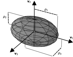
Figure 1: Representation of tensor as ellipsoid; eigenvalues $\rho_{k}$ and eigenvectors $v_{k}$ are highlighted.

Generally, the anisotropy tensor describes and measures the deviation of the Reynolds stress tensor from the isotropic state, where its geometric ellipsoid representation forms a perfect sphere ($\rho_{1}=\rho_{2}=\rho_{3}$). The invariants of the anisotropy tensor

$$\begin{split}\text{I}_{\mathbf{a}}&=\text{tr}\left(\mathbf{a}\right)=0\\ \text{II}_{\mathbf{a}}&=-\frac{1}{2}\text{tr}\left(\mathbf{a}^{2}\right)=\lambda_{1}\lambda_{2}+\lambda_{1}\lambda_{3}+\lambda_{2}\lambda_{3}\\ \text{III}_{\mathbf{a}}&=\det\left(\mathbf{a}\right)=\lambda_{1}\lambda_{2}\lambda_{3}\end{split}$$ (3)

can be used to visualize the tensor in a coordinate-system-invariant way, called the AIMhastargettrueAnisotropy Invariant Map (AIM) Lumley, in Fig. 2.

Figure 2: AIMhastargettrueAIM of the Reynolds stress tensor comparing second and third invariant of respective anisotropy tensor. The corners of the triangle (1C, 2C,3C) represent the componentiality of turbulence (see Table 1).

Because of the physical realizability constraints of the Reynolds stress tensor Schumann1977

$$\tau_{\alpha\alpha}\geq 0\ \text{,}\quad\tau_{\alpha\alpha}\cdot\tau_{\beta\beta}\geq\tau_{\alpha\beta}^{2}\ \text{,}\quad\text{det}\left(\mathbf{\tau}\right)\geq 0\ \text{,}\ \quad\alpha,\beta={1,2,3}$$ (4)

and the definition of the anisotropy tensor (see Eq. 1), the entries of the anisotropy tensor are bounded in the following ranges:

$$\begin{split}a_{ij}\in\left\{\begin{array}[]{ll}\left[-\frac{2}{3},\frac{4}{3}\right]&\text{for}\ i=j\\ \left[-1,1\right]&\text{for}\ i\neq j\end{array}\right..\end{split}$$ (5)

The eigenspace decomposition of the anisotropy tensor in combination with tensor diagonalization (see Eq. 2) leads to the fact that any physically realizable Reynolds stress tensor can be mapped to exactly one respective anisotropy tensor in its canonical form $\Lambda_{ij}=\mathrm{diag}(\lambda_{1},\lambda_{2},\lambda_{3})$. Applying Eq. 5 to $\Lambda_{ij}$, the ordered eigenvalues

$$\begin{split}\lambda_{1}&=\max_{\alpha}\left(a_{\alpha\alpha}|_{\mathrm{PCS}}\right)\\ \lambda_{2}&=\max_{\beta\neq\alpha}\left(a_{\beta\beta}|_{\mathrm{PCS}}\right)\\ \lambda_{3}&=-\lambda_{1}-\lambda_{2}=\min_{\gamma\neq\alpha,\beta}\left(a_{\gamma\gamma}|_{\mathrm{PCS}}\right)\ \text{,}\end{split}$$ (6)

are bounded accordingly Terentiev2006:

$$\lambda_{1}\geq\frac{3|\lambda_{2}|-\lambda_{2}}{2}\ \text{,}\ \lambda_{1}\leq\frac{1}{3}-\lambda_{2}\ \text{.}$$ (7)

Turbulence componentiality Terentiev2006 categorizes three fundamental states (one-, two- and three-component turbulence) based on the number of non-zero eigenvalues of the Reynolds stress tensor $\rho_{i}$ (and respective anisotropy tensor eigenvalues $\lambda_{i}$), presented in Table 1. Besides, axisymmetric turbulence is characterized by two eigenvalues being equal, while an isotropic state features three identical eigenvalues.

Table 1: Turbulence componentiality and limiting states of turbulence with respect to eigenvalues of the Reynolds stress tensor $\rho_{i}$ and the anisotropy tensor $\lambda_{i}$.

States of turbulence	componentiality	eigenvalues
	# $\rho_{i}\neq 0$ or # $\lambda_{i}\neq-\frac{2}{3}$	$\rho_{i}$	$\lambda_{i}$
One-component (1C)	1	$\rho_{1}=2k,\rho_{2}=\rho_{3}=0$	$\lambda_{1}=\frac{4}{3},\lambda_{2}=\lambda_{3}=-\frac{2}{3}$
Two-component	2	$\rho_{1}+\rho_{2}=2k,\rho_{3}=0$	$\lambda_{1}+\lambda_{2}=\frac{2}{3},\lambda_{3}=-\frac{2}{3}$
Two-component axisymmetric (2C)	2	$\rho_{1}=\rho_{2}=k,\rho_{3}=0$	$\lambda_{1}=\lambda_{2}=\frac{1}{3},\lambda_{3}=-\frac{2}{3}$
Three-component	3	$\rho_{1}+\rho_{2}+\rho_{3}=2k$	$\lambda_{1}+\lambda_{2}+\lambda_{3}=0$
Three-component isotropic (3C)	3	$\rho_{1}=\rho_{2}=\rho_{3}=\frac{2}{3}k$	$\lambda_{1}=\lambda_{2}=\lambda_{3}=0$

The corners of the AIMhastargettrueAIM in Fig. 2 can be classified as the (three-component) isotropic limit (3C), the two-component axisymmetric limit (2C) and the one-component limit (1C) (see also Table 1). Moreover, due to the boundedness of the anisotropy tensor entries (and its eigenvalues, respectively), all physically plausible states of turbulence must lie within the area spanned by the corners of the triangle. Furthermore, due to the boundedness of the anisotropy tensor’ eigenvalues, a barycentric triangle can be constructed based on the spectral theorem Banerjee2007. Consequently, every physically realizable state of the Reynolds stress tensor can be mapped onto barycentric coordinates

$$\begin{split}\mathbf{x}=&\frac{1}{2}\mathbf{x}_{\mathrm{1C}}\left(\lambda_{1}-\lambda_{2}\right)+\mathbf{x}_{\mathrm{2C}}\left(\lambda_{2}-\lambda_{3}\right)+\mathbf{x}_{\mathrm{3C}}\left(\frac{3}{2}\lambda_{3}+1\right)\\ \mathbf{x}=&\mathbf{Q}\bm{\lambda}\quad\text{with}\ \lambda_{1}\geq\lambda_{2}\geq\lambda_{3}\ \text{,}\end{split}$$ (8)

where $\mathbf{Q}$ depends on the choice of corners of the barycentric triangle. Fig. 3 shows these three limiting states of the Reynolds stress tensor, defined by the corners of the triangle ($\mathbf{x}_{\mathrm{1C}},\mathbf{x}_{\mathrm{2C}},\mathbf{x}_{\mathrm{3C}}$) representing the one-component, two-component axisymmetric and three-component (isotropic) turbulent state. A great benefit of the ABMhastargettrueAnisotropy Barycentric Map (ABM) is the possibility to obtain a linear interpolation between two points with respect to their eigenvalues. The eigenspace perturbation exploits this property as well. Hence, we will come back to it later.

II.2 Perturbation of Eigenspace Representation

As the Reynolds stresses are expressed as functions of the mean flow quantities for turbulence modeling, we need to consider the nature of their relationship. A common example are the state-of-the-art LEVMhastargettrueLinear Eddy Viscosity Models (LEVM), which assume this relationship to be linear and introduce a turbulent (eddy) viscosity $\nu_{t}$ to approximate the Reynolds stress tensor in analogy to the viscous stresses

$$\tau_{ij}=-2\nu_{t}\left(S_{ij}-\frac{1}{3}\frac{\partial u_{k}}{\partial x_{k}}\delta_{ij}\right)+\frac{2}{3}k\delta_{ij}\ \text{,}$$ (9)

where the strain-rate tensor is denoted as $S_{ij}$. In the past decades researchers have pointed out limitations of these LEVMhastargettrueLEVM for flow situations, which are not covered by the calibration cases Speziale; Mompean; CRAFT1996108; Lien. The estimated relationship between Reynolds stresses and mean rate of strain results in the inability to account correctly for its anisotropy and consequently lead to a significant degree of epistemic uncertainty. In order to account for such epistemic uncertainties due to the model-form, the perturbation approach suggests to modify the eigenspace (eigenvalues and eigenvectors) of the Reynolds stress tensor within physically permissible limits Emory; Iaccarino. The EPFhastargettrueEPF of the Reynolds stress tensor implemented in TRACE creates a perturbed state of the Reynolds stress tensor defined as

$$\begin{split}\tau_{ij}^{*}&=k\left(a_{ij}^{*}+\frac{2}{3}\delta_{ij}\right)\\ &=k\left(v_{in}^{*}\Lambda_{nl}^{*}v_{jl}^{*}+\frac{2}{3}\delta_{ij}\right)\ \text{,}\end{split}$$ (10)

where $a_{ij}^{*}$ is the perturbed anisotropy tensor, $\Lambda_{nl}^{*}$ is the perturbed eigenvalue matrix and $v^{*}_{in}$ is the perturbed eigenvector matrix. The turbulent kinetic $k$ energy is left unchanged. In the following sections, we will describe the mathematical and physical foundation of forming a perturbed eigenspace.

II.2.1 Eigenvalue perturbation

The eigenvalue perturbation utilizes the boundedness of the eigenvalues of the anisotropy tensor and their representation in terms of barycentric coordinates, as described in Section II.1. As the representation of the anisotropy tensor within the ABMhastargettrueABM enables linear interpolation between a starting point $\mathbf{x}$ and a target point $\mathbf{x}_{(t)}$, the perturbation methods creates a modified location $\mathbf{x}^{*}$, according to

$$\mathbf{x}^{*}=\mathbf{x}+\Delta_{B}\left(\mathbf{x}_{(t)}-\mathbf{x}\right)\ \text{,}$$ (11)

with the relative distance $\Delta_{B}\in[0,1]$ controlling the magnitude of eigenvalue perturbation as illustrated in Fig. 3. The starting point $\mathbf{x}$ is usually determined in the RANShastargettrueRANS simulation iteration via the relationship for the Reynolds stresses determined by the turbulence model, e.g. the Boussinesq assumption for LEVMhastargettrueLEVM (see Eq. 9). Due to their distinctive significance, the limiting states of turbulence at the corners act typically as the target point $\mathbf{x}_{(t)}\in\{\mathbf{x}_{\mathrm{1C}},\mathbf{x}_{\mathrm{2C}},\mathbf{x}_{\mathrm{3C}}\}$. Subsequently, the perturbed eigenvalues $\lambda_{i}^{*}$ can be remapped by the inverse of $\mathbf{Q}$

$$\bm{\lambda}^{*}=\mathbf{Q}^{-1}\mathbf{x}^{*}\ \text{.}$$ (12)

Figure 3: ABMhastargettrueABM representing the eigenvalues of the anisotropy tensor and its effect on the shape of the Reynolds stress tensor ellipsoid. The eigenvalue perturbation towards the two-component limiting state of turbulence is shown schematically.

II.2.2 Eigenvector perturbation

In contrast to the eigenvalues, there are no physical bounds for the orientation of the eigenvectors of the Reynolds stress tensor and there is no upper limit for the turbulent kinetic energy. Thus, the fundamental idea of perturbing the eigenvectors is to create bounding states for the production $P_{k}$ of turbulent kinetic energy $k$ in transport equation based LEVMhastargettrueLEVM . Hereby, the budget of turbulent kinetic energy is indirectly manipulated. The turbulent production term is defined as the Frobenius inner product of the Reynolds stress and the strain-rate tensor. Since both are positive semi-definite, the bounds of the Frobenius inner product can be written in terms of their eigenvalues $\rho_{i}$ and $\sigma_{i}$ arranged in decreasing order Lasserre:

$$\begin{split}P_{k}&=-\tau_{ij}\frac{\partial u_{i}}{\partial x_{j}}=-\tau_{ij}\cdot S_{ij}=-\langle\bm{\tau},\mathbf{S}\rangle_{F}=-\text{tr}\left(\bm{\tau}\mathbf{S}\right)\\ &\in\left[\rho_{1}\sigma_{3}+\rho_{2}\sigma_{2}+\rho_{3}\sigma_{1},\,\rho_{1}\sigma_{1}+\rho_{2}\sigma_{2}+\rho_{3}\sigma_{3}\right]\ \text{.}\end{split}$$ (13)

Since the Reynolds stress and the strain rate tensor share the same eigenvectors in LEVMhastargettrueLEVM (see Eq. 9), the lower bound of the turbulent production term can be obtained by commuting the first and third eigenvector of the Reynolds stress tensor, whereas maximum turbulent production is obtained by not changing the eigenvectors of the Reynolds stress tensor:

$$\begin{split}\mathbf{v}_{\textrm{max}}&=\begin{pmatrix}\mathbf{v}_{1_{\mathbf{S}}}&\mathbf{v}_{2_{\mathbf{S}}}&\mathbf{v}_{3_{\mathbf{S}}}\end{pmatrix}\rightarrow P_{k_{\textrm{max}}}\\ \mathbf{v}_{\textrm{min}}&=\begin{pmatrix}\mathbf{v}_{3_{\mathbf{S}}}&\mathbf{v}_{2_{\mathbf{S}}}&\mathbf{v}_{1_{\mathbf{S}}}\end{pmatrix}\rightarrow P_{k_{\textrm{min}}}\ \text{.}\end{split}$$ (14)

Note: Permuting of the eigenvectors of the Reynolds stress is equivalent to changing the order of the respective eigenvalues. Both change the alignment of the Reynolds stress ellipsoid with the principle axes of the strain-rate tensor.

II.2.3 Implications for CFDhastargettrueCFD practitioners

The eigenspace perturbation can be divided into eigenvalue and eigenvector modifications of the Reynolds stress tensor. For practical application purposes each eigenvalue perturbation towards one of the limiting states of turbulence can be combined with minimization or maximization of the turbulent production term (eigenvector perturbation). In summary, the model-form uncertainty of LEVMhastargettrueLEVM can be estimated by 6 additional CFDhastargettrueCFD simulations if $\Delta_{B}<1$ and only 5 perturbed simulations if $\Delta_{B}=1$ is chosen. This is because the Reynolds stress ellipsoid is a perfect sphere when targeting for the $\mathrm{3C}$ turbulence state with $\Delta_{B}=1$ (see Fig. 3), making an eigenvector perturbation obsolete. As the amount of considered turbulence model uncertainty scales with the relative perturbation strength $\Delta_{B}$, aiming for the corners of the barycentric triangle (applying $\Delta_{B}=1$) is common practice in order to obtain a worst case estimate corresponding to the most conservative uncertainty bounds on QoIhastargettrueQoI Emory; Iaccarino; MishraSU2; MathaCF. The analysis of additional CFDhastargettrueCFD simulations, propagating the effect of perturbed Reynolds stress tensor, enables a CFDhastargettrueCFD practitioner to quantify the derived effect of the turbulence model perturbation on certain QoIhastargettrue