3D hydrodynamic simulations of massive main-sequence stars II. Convective excitation and spectra of internal gravity waves

Abstract

Recent photometric observations of massive stars have identified a low-frequency power excess which appears as stochastic low-frequency variability in light curve observations. We present the oscillation properties of high resolution hydrodynamic simulations of a $25\;\mathrm{\mathrm{M}_{\odot}}$ star performed with the PPMstar code. The model star has a convective core mass of $\approx 12\;\mathrm{\mathrm{M}_{\odot}}$ and approximately half of the envelope simulated. From this simulation, we extract light curves from several directions, average them over each hemisphere, and process them as if they were real photometric observations. We show how core convection excites waves with a similar frequency as the convective time scale in addition to significant power across a forest of low and high angular degree $l$ modes. We find that the coherence of these modes is relatively low as a result of their stochastic excitation by core convection, with lifetimes on the order of 10s of days. Thanks to the still significant power at higher $l$ and this relatively low coherence, we find that integrating over a hemisphere produces a power spectrum that still contains measurable power up to the Brunt–Väisälä frequency. These power spectra extracted from the stable envelope are qualitatively similar to observations, with same order of magnitude yet lower characteristic frequency. This work further shows the potential of long-duration, high-resolution hydrodynamic simulations for connecting asteroseismic observations to the structure and dynamics of core convection and the convective boundary.

1 Introduction

Asteroseismology has evolved into a powerful tool in stellar physics, to probe stellar interiors and to validate our basic understanding of stellar physics and evolution. For example, asteroseismology has been able to constrain the extent and nature of convective boundary mixing in main-sequence stars (e.g. Aerts et al., 2003; Moravveji et al., 2015, 2016; Angelou et al., 2020; Viani & Basu, 2020; Michielsen et al., 2021; Bowman & Michielsen, 2021) and the theoretical studies suggest that even more detailed constraints may be possible in the future (Pedersen et al., 2018; Michielsen et al., 2019; Pedersen et al., 2021).

When a star’s hydrostatic equilibrium is perturbed, different kinds of oscillations can result. Familiar sound waves arise from pressure perturbations and propagate at the local speed of sound. On longer time scales, a second class of oscillation can also occur when there is a density disturbance. In this case, the force of gravity acts to counteract the over- or under-density, so they are referred to as gravity or buoyancy waves (Aerts et al., 2010). Gravity waves can occur in stratified fluids either at an interface between two disparate fluids, in which case they are called surface (or interfacial) waves, or in a continuously stratified fluid, in which case they are called internal gravity waves (IGWs). IGWs obey a dispersion relation where their wave vectors make lie at angles $\varphi$ with respect to surfaces of a constant density according to $\omega=N\cos(\varphi)$, where $N$ is the Brunt–Väisälä (BV) frequency. This quantity sets the maximum frequency at which gravity waves can propagate.

Gravity waves are important probes of stellar interiors, as they are sensitive to the physics of stellar structure and are particularly sensitive to the interior mixing and rotation profiles within massive stars (Rogers et al., 2013; Aerts & Rogers, 2015; Bowman, 2020). In asteroseismology, standing gravity waves are referred to as g modes, whereas standing pressure waves are referred to as p modes. We follow the convention that p modes are labelled with positive radial order $n$ and g modes are labelled with negative radial order $n$ (higher radial order g modes are more negative).

In massive stars, gravity waves are excited at the interface of convective and radiative regions such as the boundary of the hydrogen-burning convective core during the main-sequence phase of stellar evolution and partial ionization zones within the radiative envelope (Dziembowski & Pamyatnykh, 1993; Dziembowski et al., 1993). Since convection is a turbulent and intermittent process, the excitation is stochastic. These gravity waves have been hypothesized as significant contributors to photometric variability in massive stars, especially at low frequencies where coherent heat-driven g modes excited by local opacity enhancements in the iron-bump layer are not the dominant source of variability (Aerts & Rogers, 2015; Bowman et al., 2019a).

Recently, high-precision photometric observations of hundreds of massive stars assembled by the NASA K2 and TESS missions (Howell et al., 2014; Ricker et al., 2015) have revealed the distinct features of stochastic low-frequency variability inferred to be caused by gravity waves (Bowman et al., 2019a). From such observations, Bowman et al. (2020); Bowman & Dorn-Wallenstein (2022) demonstrated that the morphology of the stochastic low-frequency variability (i.e. dominant periodicities and amplitudes) directly probes the evolutionary properties of the host star (i.e. its mass and age).

From a stellar structure model using a given set of input physics, such as those available from the 1D evolution code MESA (Paxton et al., 2011, 2013, 2015, 2018, 2019), pulsation codes such as GYRE are able to calculate the resonant eigenmodes for various pulsation mode geometries of a stellar model (Townsend & Teitler, 2013; Townsend et al., 2018). Such calculations for a grid of models allow forward seismic modelling of stars based on a quantitative comparison of the observed and theoretically-predicted pulsation mode frequencies (Aerts, 2021). Furthermore, non-adiabatic calculations reveal the growth rate of pulsation modes and allow the excitation physics of heat (i.e. opacity) driven coherent pulsations to be probed. However, as demonstrated by recent space-based observations of massive stars, there remain large uncertainties associated with rotation and stellar opacities which significantly affect the predictions of opacity-driven coherent mode excitation (e.g. Burssens et al. 2020).

To study the excitation of gravity waves by convection, astrophysicists have turned to two and three dimensional hydrodynamic simulations (Ratnasingam et al., 2020; Horst et al., 2020; Le Saux et al., 2023; Ratnasingam et al., 2023; Anders et al., 2023). These codes directly simulate the motions and properties of fluids. Rogers et al. (2013) and Edelmann et al. (2019a) have surmised that the excitation of stochastic IGWs in massive stars is driven predominantly by convective plumes that overshoot the convective boundary between the core and the stable envelope. Some of these simulations required very high heating factors beyond the nominal luminosity of the star (on the order of $10^{6}$ times higher) and correspondingly high viscosities to maintain numerical stability. These simulations showed plumes tend to excite g modes with large wavelengths, or low angular degrees $l$.

In Paper I (Herwig et al., 2023) we presented 3D stellar hydrodynamic simulations with heating factors ranging from $10^{1.5}$ to $10^{4}$ and high grid resolution based on the explicit, compressible gas-dynamics approach using the PPMstar code. Those simulations allow us to characterize the large-scale and turbulent nature of core convection in massive stars and establish the converged excitation spectrum up to angular spherical harmonic degree $l\approx 100$.

The global flow morphology leads to boundary layer separation flows in which small-scale instabilities are generated causing perturbations. This is reflected in the flat spectrum of the radial component of convective motions near the boundary compared to a fully-developed Kolmogorov spectrum in the core region far away from the boundary.

The stable layers immediately outside the convective core host IGWs with the dominant power in the radial velocity component at radial order $n=-1$ and large wave number $l\approx 70$. These IGWs have been hypothesized as a source of mixing in the stable layers adjacent to the convective boundary (Blouin et al., 2022, and discussion there). The IGW spectrum of the horizontal velocity component follows the turbulent spectrum maintaining the familiar $\propto l^{-5/3}$ power law spectrum, whereas the radial velocity component assumes a distinctly different spatial spectrum that peaks at high wave numbers $l\approx 30\dots 70$. Reynolds stresses cause a tight correlation between the horizontal spectrum in the convection and stable layers, but a broad spectrum of radial plume-like excitations facilitate the distinct spectral morphology of the radial velocity component.

In this paper we explore the properties of IGWs further out in the stable layers and present a detailed theoretical asteroseismic analysis of three simulations with heating factor $1000\times$. The goal of this paper is to expand our analysis of IGWs from the boundary region explored in Paper I to the stable envelope further away from the boundary, and to establish the spectral properties of synthetic observations of light curves of the oscillating envelope. We are motivated by the observed asteroseismic features of massive stars such as the near-ubiquitous low-frequency variability reported by Bowman et al. (2019a), but note that our simulations do not include the outer envelope and surface that are probed by real observations, nor the effects of radiative damping. Despite these limitations, this work nonetheless aims to identify mechanisms and effects that could play a role in the origin of a spectrum with a low-frequency excess.

We begin in §2 by describing our methods including a brief account of the underlying hydrodynamic simulations, the asteroseismic analysis technique, and the GYRE analysis of the spherically averaged radial profiles for the mode identification. In §3, we present the flow morphology of convection in the core and oscillations in the envelope. Then, we present simulated synthetic light curves extracted as if we were observing the luminosity of the star partway through the radiative envelope. We perform an asteroseismic analysis of these light curves and reveal a strong low-frequency excess. From there, the remainder of the paper is dedicated to dissecting this luminosity power spectrum and explaining how its various features come to be. Finally, §4 presents discussion and conclusions.

2 Methods

Based on 3D hydrodynamic simulations of a $25\;\mathrm{\mathrm{M}_{\odot}}$ main-sequence star slightly evolved beyond the zero-age main sequence (Paper I, Herwig et al., 2023) we generate simulated observations of light curves to compare them with observations. We decompose the oscillations in three dimensions into spherical harmonics, and compare them with eigenmodes calculated using GYRE to identify specific IGW modes.

2.1 Hydrodynamic simulations

Table 1: The most important simulations from Paper I analyzed in this paper. Additional simulations featured only in §3.5 are described in detail in Paper I. The table provides the run name, the grid size, number of dumps (see details on PPMstar dumps in Paper I), total length of run in simulated star time.

Name	Resolution	Dumps	Duration
M107	$768^{3}$	9943	$290\;\mathrm{\mathrm{d}}$
M114	$1152^{3}$	5926	$170\;\mathrm{\mathrm{d}}$
M115	$1728^{3}$	3584	$103\;\mathrm{\mathrm{d}}$

The simulations used here are summarized in Table 1 and described in more detail in Paper I. The simulations have been performed with the PPMstar gas dynamics code (Woodward et al., 2015; Jones et al., 2017; Andrassy et al., 2020; Stephens et al., 2021), with several important updates. The most relevant for this work relates to PPMstar now solving the conservation laws in terms of perturbations with respect to a base state which aids computational accuracy. It also makes the mapping of a 1D stratification from a stellar evolution code to 3D substantially easier and results in an initial 3D stratification that is by definition in hydrostatic equilibrium. At the bounding sphere we impose a reflecting boundary condition using ghost cells that mirror the cells across the bounding surfaces (see section 2.2 in Paper I for details).

In our $25\mathrm{M}_{\odot}$ simulation, the convective boundary is located at $\approx 1500\mathrm{M}\mathrm{m}$ on top of which is a stable envelope with a radial extent of $1200\mathrm{M}\mathrm{m}$. The MESA model has a radius of $5000\mathrm{M}\mathrm{m}$ and therefore the simulation includes $54\%$ of the star’s radius. Since we dedicate a significant fraction of our resolution budget to the core, the simulations resolve the large-scale flows and turbulence, as well as interactions between convective flows and the boundary. This allows the simulation to accurately capture the excitation process. We include enough of the stable envelope to probe oscillation properties several pressure scale heights away from the convective boundary without getting close to the outer edge of the simulation domain.

The base state of the 3D hydrodynamic simulations approximates the structure of a $25\;\mathrm{\mathrm{M}_{\odot}}$ stellar evolution model calculated with the MESA stellar evolution code (Davis et al., 2019, template run). Details are provided in Paper I. The model star is near the zero-age main-sequence, $1.64\times 10^{6}\mathrm{yr}$ after the start of H burning, and its central H mass fraction has decreased to $X(\mathrm{H})_{\mathrm{c}}=0.606$ from the initial $0.706$.

The three simulations differ by grid resolution. In all cases the output (dump) cadence is $\approx 43\mathrm{min}$, which is comparable to the observational cadence of the 30-min (“long-cadence”) observing mode of the K2 and TESS planet-hunting satellites (Howell et al., 2014; Ricker et al., 2015). The $768^{3}$ simulation M107 was followed for slightly over nine months of simulated time. The long baseline and correspondingly high resolution for low frequencies allow at least qualitative comparisons to asteroseismic observations. However, with regard to some mixing properties this grid resolution is not entirely sufficient. Simulation M114 with a $1152^{3}$ grid still follows $170\;\mathrm{\mathrm{d}}$ of simulated time and is ideal to study the internal structure of the star and its oscillations. The M115 simulation was performed on a $1728^{3}$ grid for $103\;\mathrm{\mathrm{d}}$ containing over five billion grid cells and is used to determine the convergence properties of the oscillation results.

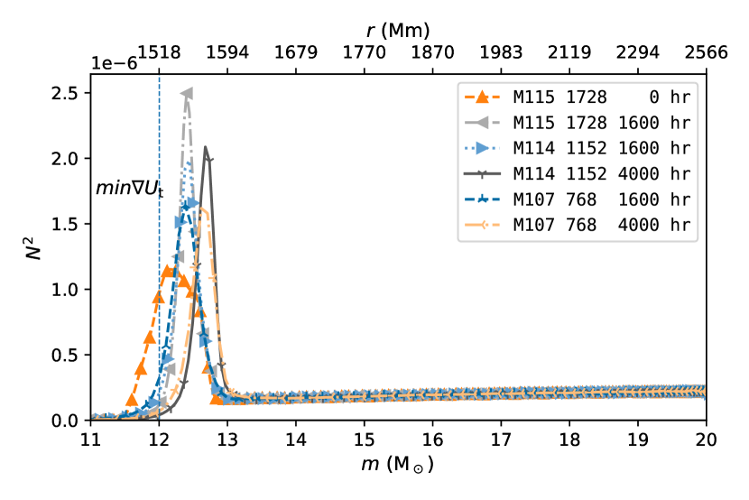
Figure 1: Profile of BV frequency for the three simulations. $N^{2}$ has been calculated from the spherically averaged profiles of the 3D hydrodynamic simulations. The labels indicate the run ID, the grid resolution and the time of the simulation for which each profile is shown. The vertical dashed line indicates the location of the minimum gradient of the tangential velocity component for run M107, $t=1600\mathrm{h}$ which is discussed in Paper I as one criterion to define the convective boundary. $N$ has units of the angular frequency $\mathrm{rad\ s^{-1}}$.

The Brunt–Väisälä frequency profile of the adopted base state and its changes during subsequent simulation run-time are shown in Fig. 1. Despite applying a heating factor of $1000$ which makes the convective flows $10\times$ faster compared to nominal heating, the flows remain very slow. It takes about $40\;\mathrm{d}$ of simulated time until a steady state is reached. By then, it has established a convective boundary profile due to hydrodynamic processes only. This can be seen in the evolution of the $N^{2}$ peak profile in Fig. 1 (cf. Fig. 15 in Paper I). At higher resolutions, the maximum of the $N^{2}$-peak is larger and the boundary region is narrower. In the real star the shape of the $N^{2}$-peak in the boundary is the convolution of its dynamic-, thermal-, and nuclear-time scale evolution. The base states we adopted for these simulations reflect the convective boundary mixing assumptions adopted in the MESA stellar evolution model and may have to be revised in future. Note that the values in Table 1 are the total simulated time, including the initial transition period.

Fourier analysis of the oscillations requires a long duration baseline, but we nonetheless avoid the initial phase in which the $N^{2}$ boundary is changing because it might affect details of the wave excitation. We therefore exclude the initial $1300$ dumps ($930\mathrm{h}$) from the analysis.

As the simulations run, the following data are output for later analysis. Rendered images of the simulation are created from full resolution two-dimensional outputs at each dump (Fig. 3; Section 2.2 of Paper I for details). Likewise, one dimensional radial profile outputs prepared by the simulation code are based on uncompressed, full resolution data at the time of each dump. This includes asteroseismic observables (Fig. 4). Analysis of the three dimensional structure of the simulation, on the other hand, is carried out against reduced resolution data (that we call briquette data, see Stephens et al., 2021, for details) that contains three dimensional outputs of some quantities with a resolution reduced by a factor 4 in each direction but full 4-byte precision. The decomposition of oscillation motions into spherical harmonics is based on this type of filtered output data.

2.2 Asteroseismic analysis

The PPMstar code generates simulated observations of the luminosity fluctuations by first calculating the bolometric radiance $L$ of each octant of each grid cell using its temperature and treating it as a black body. These simulated observations are generated at each radius in the simulation up to $54\%$ of the radius of the star. The luminosity is instead reported at mass coordinates up to $m_{\mathrm{r}}=20\;\mathrm{\mathrm{M}_{\odot}}$.

Eight different vantage points from which the simulated star might be observed are chosen not to align with the simulation grid. The first four lines of sight (los) to the star are chosen to be along:

$$\overrightarrow{\mathrm{los}_{1}}= (1,1,1)$$

$$\overrightarrow{\mathrm{los}_{2}}= \overrightarrow{\mathrm{los}_{1}}\times(0,0,1)$$

$$\overrightarrow{\mathrm{los}_{3}}= \overrightarrow{\mathrm{los}_{1}}\times\overrightarrow{\mathrm{los}_{2}}$$

$$\overrightarrow{\mathrm{los}_{4}}= \overrightarrow{\mathrm{los}_{1}}+\overrightarrow{\mathrm{los}_{2}}+\overrightarrow{\mathrm{los}_{3}}$$

Each vector is normalized before it is used to define the others. The subsequent four are anti-parallel to the first four, i.e. $\overrightarrow{\mathrm{los}_{5}}=-\overrightarrow{\mathrm{los}_{1}}$ and $\overrightarrow{\mathrm{los}_{6}}=-\overrightarrow{\mathrm{los}_{2}}$, etc. This choice allows us to examine the simulation from all sides and avoids grid-alignment. The radiance $L$ is integrated over one hemisphere for each line-of-sight  and for each radius. We apply Lambert’s factor $\cos(\theta)$ where $\theta$ is the angle between the surface normal and the line-of-sight. This factor changes the surface integral into an integral over the projected face of the star, mimicking an observation of an unresolved point source (though of course, we do not simulate the surface and the boundary condition is different between the simulation and a real star).

This surface integral is evaluated by computing the volume integral of $L\cos(\theta)$ in one hemisphere of a thin shell divided by its thickness at each radius. This is repeated at every dump of the simulation, giving a time sequence of eight simulated photometric observations at every radius. In §3.4.2 we demonstrate the impact of applying Lambert’s cosine factor which deemphasizes the outer annulus of the integration, and thereby the contribution of modes with high angular degree $l$. We also demonstrate how approximating the full sphere integral with just one point on the hemisphere (see for example Edelmann et al., 2019a) overemphasizes the power at frequencies just below the BV frequency.

In long duration simulations there is a slow expansion of the core. To account for this we work in Lagrangian coordinates converting our radial luminosity profiles into mass coordinates at each time step. For each simulation run, we analyze the time series luminosity data as if they were real observations of a star. As noted in Paper I, these simulations neglect the effects of radiation. As heat is added in the core, the luminosity throughout the star slowly increases. We begin by removing this trend to the luminosity.

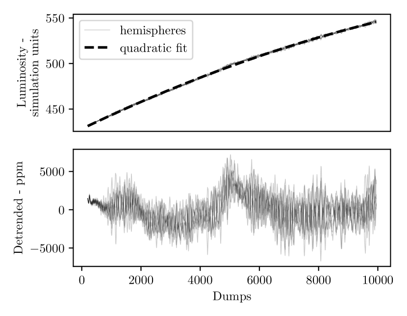
Figure 2: We take out the global luminosity trend (top panel) by fitting a quadratic to the average of all eight lines of sight. Dividing the luminosity time series from each line-of-sight by this fit gives the relative luminosity. The time axis is in units of dumps which are written out with a frequency of $\frac{1}{43\;\mathrm{\mathrm{min}}}$. The second panel shows the unity-subtracted fluctuations in luminosity compared to the quadratic fit.

Fig. 2 shows how we detrend the integrated luminosity curves at each mass coordinate by fitting a quadratic, and dividing through to arrive at the relative luminosity. We then apply a Hanning window function to impose a periodic boundary condition and control spectral leakage, and take discrete Fourier transforms of each time series to arrive at power spectra (Fig. 4). We correct the amplitude spectra for power lost due to the window function. In the simulations listed in Table 1 the default dump frequency is approximately $370\;\mathrm{\mathrm{\mu{}Hz}}$.

These light curves and their resulting spectra may appear different since they have none of the typical noise sources present in real observations such as read noise or photon noise. The only noise source present is numerical noise, which as we will see in §3.5, does not significantly effect our study. As a result, certain subtle effects like spectral leakage may be visible. For this same reason, we believe it is valid to interpret signals close to the Nyquist limit and to the minimum resolvable frequency (besides the very lowest frequencies that we have removed with our luminosity detrending).

To investigate differences and similarities to observed spectra (§3.2.3 ) we re-produce the procedure applied to real time-series photometric observations of massive stars (e.g. Bowman et al. 2019a), we apply the method known as iterative pre-whitening (Degroote et al., 2009; Pápics et al., 2012; Bowman, 2017). As an iterative procedure, we identify the frequency and amplitude of the highest-amplitude and statistically significant peak in the amplitude spectrum of the light curve, optimise the frequency, amplitude and phase using a non-linear least-squares fit to the light curve using

$$\Delta\,m=A\,\cos\left(2\pi\nu\left(t-t_{0}\right)+\phi\right)$$ (1)

where $A$ is the amplitude, $\nu$ is the frequency, $\phi$ is the phase, $t$ is the time with respect to a zero-point $t_{0}$. The optimised sinusoid is then subtracted from the light curve to produce a residual light curve. From the residual light curve, a residual amplitude spectrum is calculated and the next iteration proceeds. In the study of coherent pulsation modes in intermediate- and high-mass stars, it is typical to continue iterative pre-whitening until an amplitude signal-to-noise (S/N) criterion is satisfied. Here we use the common value of an amplitude S/N $\geq 4$ to determine if a peak is significant, in which the noise is calculated using a $1^{-1}\;\mathrm{d}$ window centred at the frequency value of extracted peak at each iteration. In this way, our iterative pre-whitening procedure only excludes the few dominant high-amplitude peaks in the amplitude spectrum, which lie on top of the low-frequency power excess background (Bowman et al., 2019b).

To follow the same methodology as applied to observations, we fit the model

$$\alpha(\nu)=\frac{\alpha_{0}}{1+\left(\frac{\nu}{\nu_{\rm char}}\right)^{\gamma}}+C_{\rm w},$$ (2)

where $\alpha_{0}$ is the amplitude at zero frequency, $\gamma$ is the logarithmic amplitude gradient, $\nu_{\rm char}$ is the characteristic frequency, and $C_{\rm w}$ is a frequency-independent (i.e. white) noise term (Bowman et al., 2019b) using a least-squares regression fit to the logarithm of the residual (i.e. post iterative pre-whitening) simulation data. This model thus yields $\nu_{\rm{char}}$ and $\gamma$ that can be directly compared to their observed counterparts.

To produce spectrograms, also known as sliding Fourier transforms, we divide the time series into sub-sequences 512 dumps in length that advance one dump at a time. We apply a Hanning window to each sub-sequence and take the Fourier transform to arrive at low resolution amplitude spectra. These amplitude spectra are then stacked according to the time at the middle of the sub-sequence to reveal how modes change over time. To reveal pertinent features, we will show the power relative to a smoothed background spectrum.

2.3 Wavenumber-frequency decomposition

We generate wavenumber-frequency $l-\nu$ diagrams from the briquette data (Stephens et al., 2021) to decompose oscillations into both spatial and temporal frequencies as a post-processing step. Since we are working with the modes of a spherical object, we choose to compute the power using a spherical harmonic basis (i.e. with discrete spherical harmonic degree $l$ instead of continuous, replacing wavenumber $k$). For each mass coordinate of interest, we sample points across a regular grid of $\theta$ and $\phi$ angular coordinates using a trilinear interpolation. Although the longest runs include almost $10\,000$ dumps corresponding to $>54$ convective turnover times, we use only $2000$ dumps for the frequency wavenumber analysis. This is because the convective boundary is migrating (cf. §3.2.2 and Paper I) which may cause artefacts if a longer baseline is used. In our spectra the frequency resolution is therefore $0.185\;\mathrm{\mathrm{\mu{}Hz}}$.

We perform the spherical harmonic decomposition using the SHTools library (Wieczorek & Meschede, 2018). We decompose the radial component of the velocity field first into complex spherical harmonic coefficients for each time step. Next, we apply a Hanning window along the time axis to control spectral leakage. Finally, we take the discrete Fourier transform of each time series of spherical harmonic coefficients. To calculate the relative luminosity fluctuations, we divide the spherical harmonic coefficients by the time-averaged $l=0$, $m=0$ coefficient for each radius. No windowing function is required along the spatial axes since the boundary conditions are naturally periodic. Finally, we use the SHTools library to calculate the power spectral density of the radial velocity oscillations normalized by degree $l$ for each frequency bin. The spherical harmonic transform and Fourier transform are both linear, so we can apply them in either order. For high-resolution runs such as M115, this post-processing step requires parallelization on a computer cluster.

The power by frequency, degree $l$, and mass coordinate represent a reduction from four dimensions to three. The resulting data cube can be sliced by mass to give frequency-wavenumber diagrams at each radius, or by $l$ to identify specific modes.

2.4 Eigenmodes of the spherically-averaged radial stratification

We use the stellar oscillation code GYRE (Townsend et al., 2018; Townsend & Teitler, 2013) to identify the eigenmodes of waves based on the spherically averaged radial stratification of the 3D simulations. In this way we can identify modes and features in the $l-\nu$ diagrams extracted from the 3D simulations as described in §2.3. GYRE solves a two-point boundary value problem for the sets of the standard equations of stellar oscillations for the adiabatic and non-adiabatic cases with an option to include rotation. We consider the case of linear adiabatic non-radial oscillations for which the governing differential equations are summarized in Appendix A of Townsend & Teitler (2013). The code uses a novel Magnus Multiple Shooting numerical scheme to find eigenfrequencies of oscillations and their corresponding eigenfunctions representing radial displacement and Eulerian perturbations of pressure and gravitational potential. GYRE is an open source Fortran code that uses OpenMP directives for parallel computations on multiple cores. It offers several integrators of differential equations among which we have chosen the fourth-order Mono-Implicit Runge-Kutta method as the most stable for our model.

We transform state variable radial profiles from the hydrodynamic simulation dumps to the MESA format readable by GYRE. Because the hydrodynamic model has an insufficient number of radial zones for the GYRE code to work well, we map it into a larger number of radial zones of its corresponding MESA model using the Akima spline interpolation. For the outer boundary condition in our GYRE calculations we used the vacuum condition with a zero pressure at the surface.

We run the GYRE code for the harmonic degree $l$ ranging from 1 to 45 to identifity the resonant g mode oscillations of radial orders $-20\leq n\leq-1$, f modes, and low-radial order p modes. The selected ranges of $l$ and $n$ numbers are determined by the successfulness of our GYRE computations. From these computations we get the eigenfrequencies $\nu$ of oscillation modes and their corresponding radial $\xi_{r}$ and horizontal $L\xi_{\mathrm{h}}$ displacement amplitudes for a given dump of our hydrodynamic simulations, where $L=\sqrt{l(l+1)}$.

3 Results

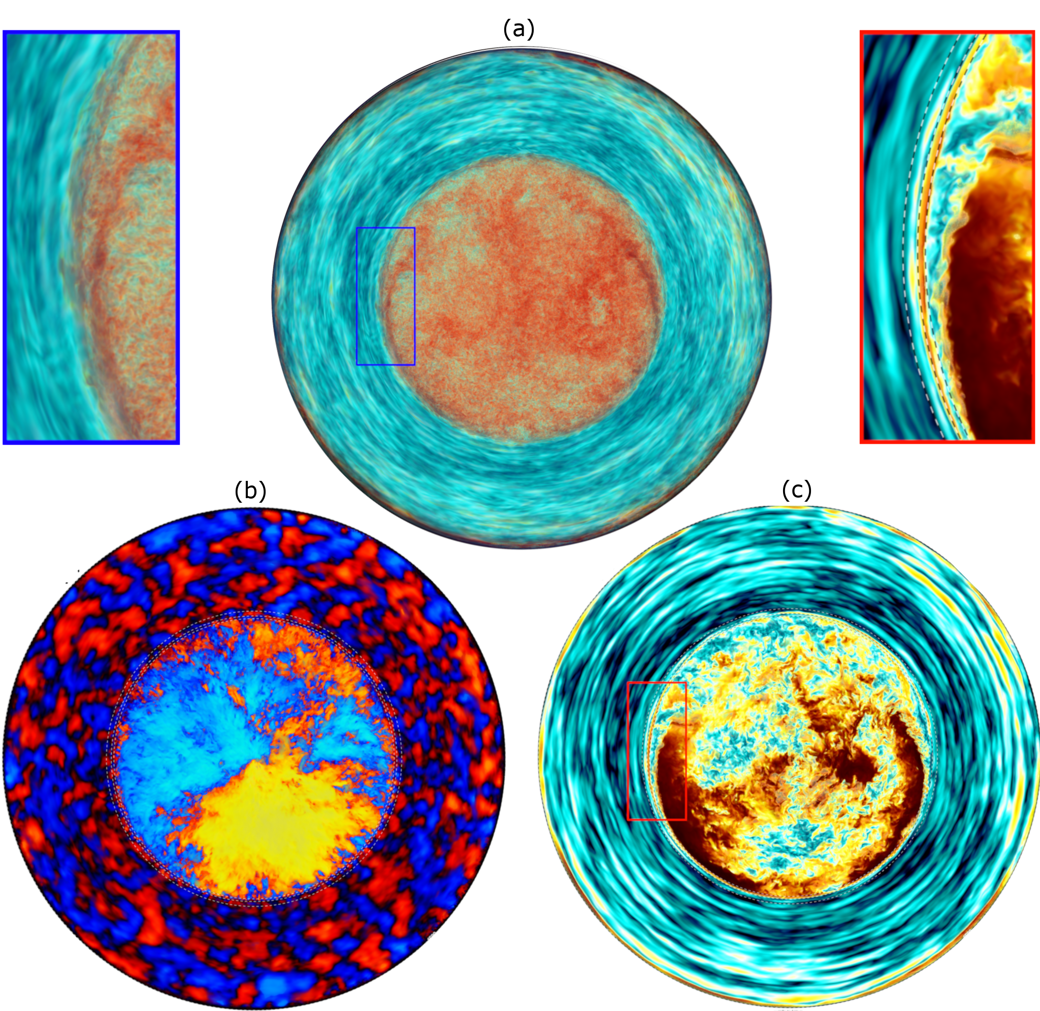
Figure 3: Centre-plane slice renderings from dump 1500 of run M115. (a) Vorticity. The color scheme has vorticity magnitude decreasing red, yellow, light and dark blue. (b) Radial velocity. The color scheme has radial velocity light to dark blue represent decreasing negative velocity magnitudes that are directed inward, yellow-orange-red represent decreasing positive radial velocity components. (c) Tangential velocity magnitude. The color scheme has tangential velocity magnitude decreasing from dark brown, red, yellow, white, light and dark blue. The white-black dashed circles have been added at the positions of $\min\bm{\nabla}|U_{\mathrm{t}}|$ (see Section 4.3 in Paper I), the radius $r_{\mathrm{N^{2}-peak}}$ where $N^{2}$ has a maximum and $r_{\mathrm{N^{2}-peak}}+0.15\mathrm{H_{P0}}$. Full resolution images and movies for runs M114 and M115 are available at https://www.ppmstar.org.

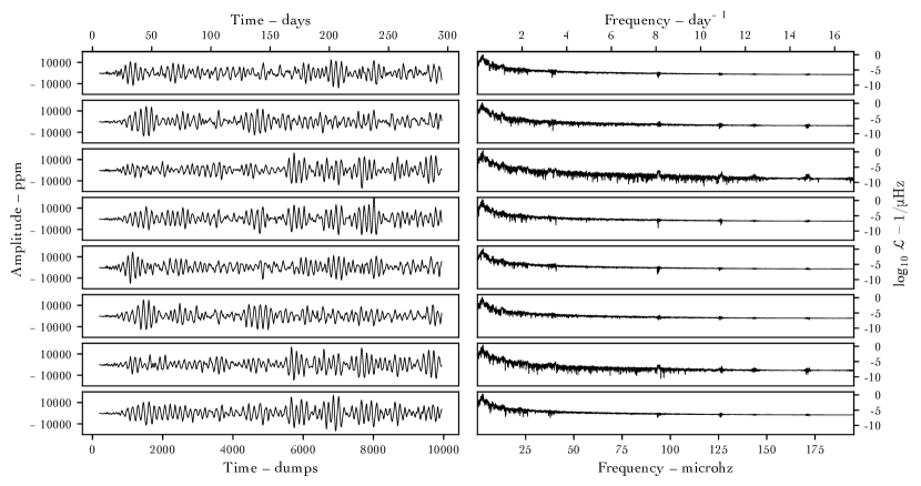
Figure 4: From top to bottom, eight simulated light curves (left panels) and their Fourier transforms (right panels) for different lines of sight of the simulation M107. The light curves are hemispheric integrations as described in §2.2. For these measurements, a radius corresponding to $19.5\;\mathrm{\mathrm{M}_{\odot}}$ was treated as the surface. The light curves have been de-trended by dividing out a quadratic fit (Fig. 2). The time unit along the bottom horizontal axis is dumps, which are written out with a frequency of $\frac{1}{43\;\mathrm{\mathrm{min}}}$. The amplitude axis plots the unity-subtracted luminosity divided by the fitted quadratic trend, in order to represent the change in luminosity amplitude in parts per million. The variable $\mathcal{L}$ is the power spectral density of the unity-subtracted, relative luminosity. Oscillations are plainly visible in first column. The second column, shown on a logarithmic scale, shows the distribution of power by frequency. The first $36\;\mathrm{d}$ of the simulation are are part of the initial transition period and omitted, see discussion in §3.2.2 regarding the inital phase of the simulation.

We present the results of our simulations and our analysis in the following order. First, we describe the general morphology of the simulations, such as the convection, the interaction with the convective boundary, and characteristics of oscillations directly visible in snapshots of the simulations. Next, we present oscillation properties of the simulation run M107 ($768^{3}$ grid) including light curves, luminosity power spectra, and the evolution of modes with time. Then, we decompose the oscillations in the simulation M114 ($1152^{3}$ grid) to reveal the breakdown by frequency and angular degree, the radial extent of each mode by mass coordinate, and the power spectrum responsible for exciting the waves. Finally, we compare the dispersion relations of our simulations to the predictions from GYRE to identify the nature of the oscillations in our simulations and to determine their specific mode numbers. We discuss the coherence time of g modes in our simulations based on the spectral line broadening and finally discuss the processes contributing to the formation of a stochastic low-frequency variability in the amplitude spectra of luminosity time series.

3.1 General morphology

The general flow morphology of the core-convection and envelope-wave fluid motions in our simulations are discussed in detail in Section 3 of Paper I. Here we summarize the most important points. Fig. 3 shows images of the vorticity, radial, and tangential velocity components for run M115 with $1728^{3}$ grid. The large-scale convective motions in the core are arranged like a giant dipole. At the time depicted in these figures, it is aligned from the north-east to the south-west direction. The radial velocity component shows inflow broadly in the top hemisphere and outflow in the bottom hemisphere representing a flow through the centre of the simulated star. In the horizontal velocity panel, the open (to the north-east) horseshoe-shaped tangential velocity arching along the boundary of the south-western hemisphere represents the return flow. We do not observe many smaller plumes impacting the convective boundary.

Instead, as the outgoing flow (panel b, red is positive radial velocity) in Fig. 3 impinges on the convective boundary, it is redirected into a sweeping tangential motion (panel b) back towards the antipode where opposing flows create a mutually adverse pressure field. Roughly $2/3$ to $3/4$ of the way around the boundary, the flow against the adverse pressure gradient starts to separate from the boundary and curls inwards to form the inflow of the dipole. As it does so, it produces a characteristic feature when projected in three dimensions like in Fig. 3. We call these boundary-layer separation wedges. They are most clearly seen in the vorticity and tangential velocity panels just inside the convective boundary in the north-west and south-east direction.

The vorticity is enhanced inside the wedges indicating additional instabilities generated due to the boundary-layer separation process, and it is here that most of the entrainment takes place due to these wedge instabilities (for details see Paper I). We have already identified and described the entrainment at the top of a convection zone through the boundary-layer separation mechanism in high-resolution simulations of He-shell flash convection in low-mass stars (Woodward et al., 2015, especially Fig. 10 and 11). Movies reveal more clearly than still images that these wedges launch waves into the stable layers. The features in the wedges are small compared to the largest convective scales like the dipole flow. Movies do not always show the convective dipole flow and the boundary-layer separation wedges clearly since the dipole axis migrates around, and may at times appear pole-on. For the images shown in Fig. 3, we selected a time where the dipole was aligned with the image rendering plane.

Focussing now on the convective boundary just above the core, ripples propagate along the interface, appearing to emanate from the flanks of the wedges. They travel along the boundary in predominantly the same direction as the flow from the wedges. At the inflow side of the dipole convection, the boundary waves are traveling in opposite directions and can be seen hitting each other, and exciting motions with finer scales. In Paper I we discussed how the immediate boundary layer where the peak of $N^{2}$ is located contains IGWs that have radial velocity components with power mostly with radial order $n=-1$ and high spherical harmonic degree $l$. Careful inspection of the shell regions around the radius $r_{\mathrm{N^{2}-peak}}$ indicated by dashed circles in Fig. 3 reveals these waves especially in the tangential velocity component along the north-western outer wedge rim, as well as on the opposite side on the outer wall of the south-east wedge.

Above the convective boundary are patterns of repeating, oscillatory motion in all velocity components. In the tangential velocity component these appear as long arcs of variable length and radial extent of $\approx 120\;\mathrm{\mathrm{M}\mathrm{m}}$. In the radial velocity component coherent patterns have substantially shorter angular extent than in the tangential velocity component and they have typically a radial extent that is twice the radial extent of the arcs in tangential components. The vorticity naturally shows smaller-scale features of the motions in the stable envelope. However, the vorticity does not show the irregular distribution of vortex-tubes that is characteristic for turbulence and clearly seen in the core. These regular velocity patterns represent wave motions that are excited by the core convection, as that is the only mechanism present in these simulations. These oscillations are predominantly larger and longer period compared to the fine structures rippling along the convective boundary.

We return to examine these waves quantitatively in §3.3. For a more complete discussion on convection, wedges, their interaction with the convective boundary, and mixing, see Paper I.

3.2 Photometric variability

We now present light curves extracted from simulation M107.

3.2.1 Simulated light curves

The eight light curves corresponding to different viewing angles of the star (cf. §2.2), taken at mass coordinate $19.5\;\mathrm{\mathrm{M}_{\odot}}$ are shown in Fig. 4. A prominent periodicity of approximately $2.5\;\mathrm{\mathrm{\mu{}Hz}}$ dominates the oscillation. This periodicity appears in each line-of-sight. In addition, the light curves show complex and irregular patterns of fluctuating amplitudes and additional frequencies can be identified. The oscillation patterns are stochastic and can be understood as the superposition of waves with a broad and fluctuating spectrum of modes. Importantly, the contribution of individual modes is variable leading to fluctuations of the amplitudes of the resulting total oscillation. The variable nature of the oscillation modes and the corresponding stochastic excitation of IGWs is discussed in detail in §3.2.2. The oscillation fluctuations are only weakly correlated or even uncorrelated for the different directions in the same hemisphere. Opposite directions are in general more correlated with each other than different directions in the same hemisphere.

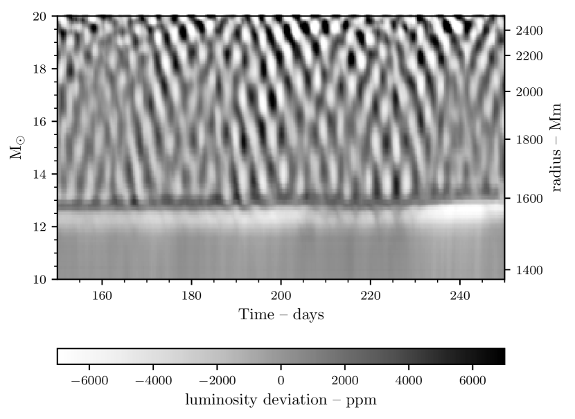
Figure 5: The evolution of the simulated photometry as a function of radius and time. The convective-boundary region begins at approximately $12\mathrm{M}_{\odot}$. Above this, oscillations are visible throughout the envelope. By visual inspection of the peaks and troughs going outward from the convective boundary, we can identify a prominent mode with radial order $n\approx 5$.

The second column of Fig. 4 shows the power spectrum corresponding to each time series. The spectra contain a rich assortment of peaks, with the highest power near $2.5\;\mathrm{\mathrm{\mu{}Hz}}$. Sharp features near 25, 95, 127, 150, and $170\;\mathrm{\mu{}Hz}$ visible from all lines of sight are p modes (see §3.3 and Fig. 13 for identification). These spectra also show that there is generally more power at lower frequencies. Below $\approx 50\;\mathrm{\mathrm{\mu{}Hz}}$ the spectrum shows more power than above. Thus, the oscillation spectra have a low-frequency excess to be discussed in more detail in §3.2.3. The sharp features visible in right panel where it may appear there is a line with a deficit of power are in fact the sidelobes of positive peaks, and are an artifact of plotting the spectrum on a log scale with little no instrumental or photon noise to hide these effects.

Considering only one light curve, we plot the time evolution of the luminosity as a function of radius in Fig. 5. This representation emphasizes the stark difference between the regular wave patterns involving radial scales of $100$ to $200\;\mathrm{\mathrm{M}\mathrm{m}}$ in the stable envelope and the turbulent noise in the convection zone. Since we integrate the light curve over one side of the simulation, the random turbulent motion averages away. The regular patterns at mass coordinates $\gtrapprox 13\;\mathrm{\mathrm{M}_{\odot}}$ represent standing waves, and again the irregular or stochastic fluctuation of the wave amplitudes in the envelope is evident.

3.2.2 Stochastic spectrum variability

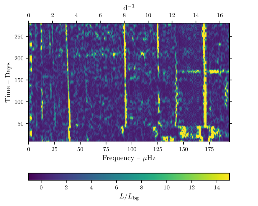
Figure 6: A sliding Fourier transform, or spectrogram, of the luminosity time series from one line-of-sight. The colour scale shows the luminosity power spectral density divided by a smooth background created by median filtering the power spectrum. Some modes are steady over time, while others are periodically re-excited such as the mode at $\approx 2\mathrm{\mu{}Hz}$. The initial transient is visible in the first $\approx 40\;\mathrm{d}$ of the simulation, which are excluded from further analysis. The window size is $15.3\;\mathrm{\mathrm{d}}$ and we advance advance each row in time by $11.5\;\mathrm{\mathrm{d}}$.

In Fig. 4, we see an apparently random variation in the power of most modes along each line of sight on the time scale of roughly $30\;\mathrm{d}$, which we call stochastic variability. For example, the 6th and 7th line of sight include periods of activity that seem uncorrelated with each other and with those at other times. The stochastic variability in integrated light is the result of the superposition of a spectrum of modes excited sporadically by core convection. This is visible most clearly in a spectrogram (Fig. 6) which shows the relative variation of power with respect to a smoothed background spectrum. Many prominent modes vary in power or frequency over the length of the simulation.

During the initial transition period of approximately one month, the core-envelope boundary ($N^{2}$-peak) migrates outward from the location defined in the initial setup (see Paper I, section 3.1.3 and 4.1 for details). After that time the $N^{2}$-peak shape does not change much and only continues to migrate outward slowly in mass and radius. Fig. 6 shows that during this initial transition period the dominant coherent modes are slightly different than at later times reflecting that the spectrum probes the shape of the $N^{2}$ profile. We generally excluded this transition period from our analysis. Note that this initial transition period is different from the much shorter initial transient time of about one convective time scale(§3.2.4) during which the velocity flow field in the convection zone and in the wave region reaches a dynamical steady-state (Paper I, section 3.1.3).

Power at some frequencies like $\approx 4\;\mathrm{\mathrm{\mu{}Hz}}$, periodically fade before being re-excited. Another example of a somewhat fainter mode can be found at $\approx 21\;\mathrm{\mathrm{\mu{}Hz}}$ which is at high power from $\approx 110$ to $150\;\mathrm{\mathrm{d}}$, then becomes weaker and is excited again at $214\;\mathrm{\mathrm{d}}$ for a duration of about $51\;\mathrm{\mathrm{d}}$. Our analysis suggests that power fluctuations shown in Fig. 6 on time scale as short as $3\;\mathrm{\mathrm{d}}$ are representative of the underlying data (cf. §3.4 for an estimate of the IGW coherence time based on the spectral line width presented below).

A sufficiently long spectrogram with a short window size, such as $15.3\;\mathrm{\mathrm{d}}$ in Fig. 6 can reveal spectral changes as a function of time, for example due to the migration of the boundary and by the adjustment of the spherically averaged structure due to heating without radiative transport. Modes in Fig. 6 migrate slightly over the duration of the simulation. For example, one mode that starts at $50\;\mathrm{\mathrm{d}}$ and $39.67\mathrm{\mu{}Hz}$ shifts to $36.95\mathrm{\mu{}Hz}$ at the end of the simulation. This could be caused by the convective boundary moving and by the adjustment of the spherically averaged structure due to heating without radiative transport and heat loss at the outer simulation boundary. We conclude that such dependency of the spectral features on the omission of radiation diffusion and the impact of this assumption on the structure is minor. This is also supported by the GYRE prediction error bars discussed at the end of §3.3.2.

Stochasticity requires not only a stochastic excitation mechanism but also some form of de-excitation or damping. After the initial transient, the tangential and radial velocity approaches a steady state, as seen in Figs. 7 and 8 of Paper I. Since these simulations do not contain the effects of radiative damping, nor significant numerical damping, a possible mechanism for damping or de-excitation in these simulations is that convection is not only a source but also a sink of wave energy. Depending on the phase of the wave and convective motions at the convective boundary where these two types of motions interface wave energy can be returned to the convection zone. In this picture the convective and wave energy content of the simulation assume an equilibrium according to the wave energy excitation and de-excitation efficiencies.

3.2.3 Low-frequency excess

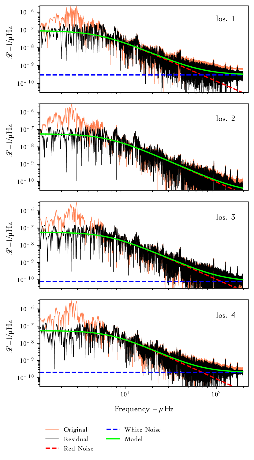
Figure 7: Fourier transforms of the photometric variability extracted from simulation M107, for four of the eight different lines of sight (los.) to the star. The variable on the vertical axis, $\mathcal{L}$, is the power spectral density of the unity-subtracted, relative luminosity. All time series were extracted at mass coordinate $19.5\mathrm{M}_{\odot}$. The orange lines are the original spectra, and the black lines are after applying iterative pre-whitening. The result is fit to the model described in §2.2.

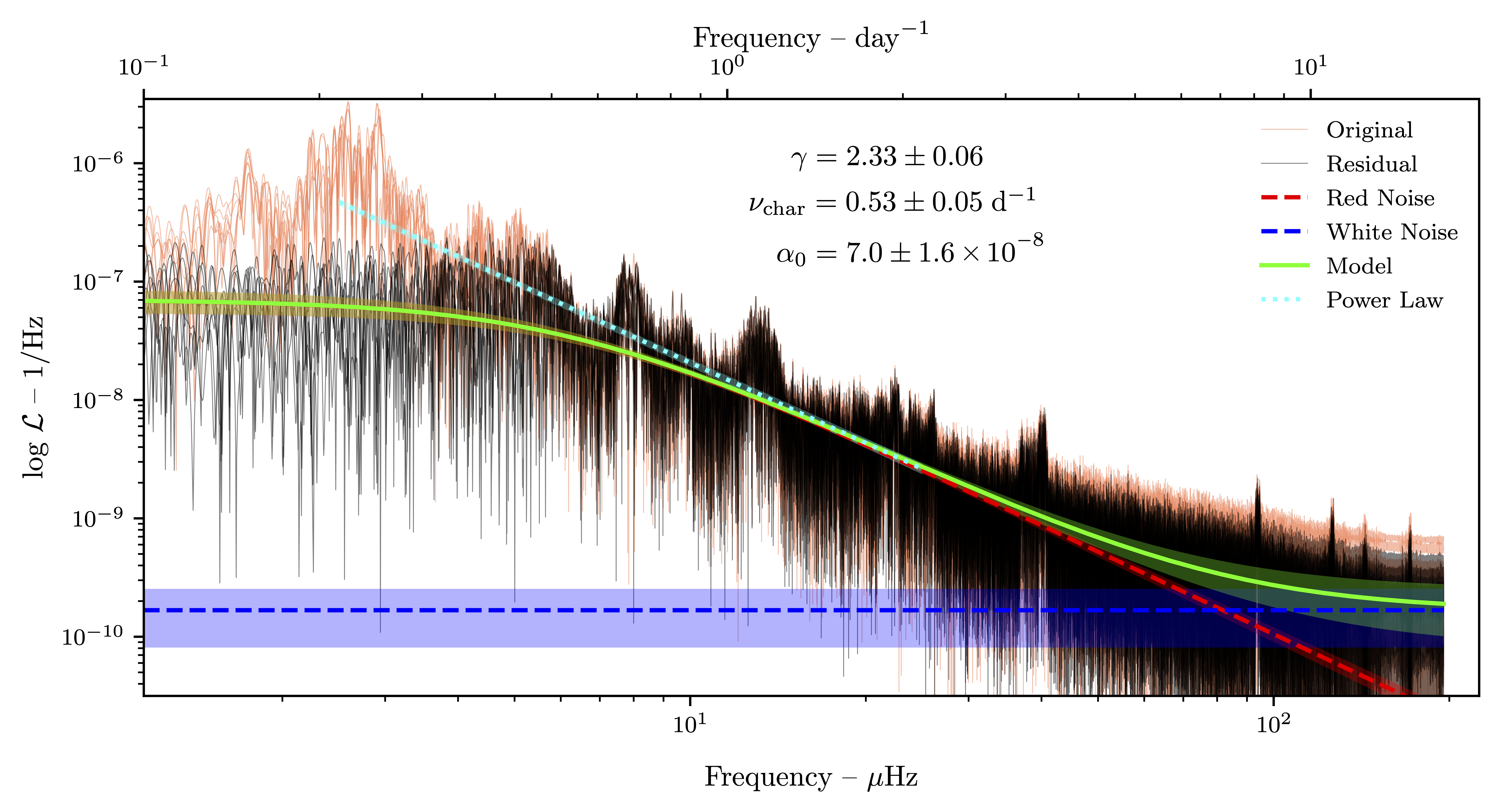
Figure 8: Superimposed luminosity power spectra (M107) of all eight lines of sight at a mass coordinate of $19.5\mathrm{M}_{\odot}$. As in Fig. 7, $\mathcal{L}$ is the power spectral density of the unity-subtracted, relative luminosity. We observe an excess of low-frequency power. The original spectra are shown in orange, and the pre-whitened spectra are shown in black. We over plot the mean of the best fitting models of each residual spectrum in green, with standard error between models marked by the shaded regions. The red and white noise components of the model are separately plotted in red and blue respectively. We also show a power law fit to the original, not pre-whitened data in cyan.

Taking the discrete Fourier transforms of these light curves leads to the eight panels in the right column of Fig. 4. These are the power spectra of relative luminosity variations, where the luminosity results from hemispheric integration and applying Lambert’s cosine factor. The power peaks at a period corresponding to a frequency of $2.5\;\mathrm{\mathrm{\mu{}Hz}}$ or $0.22\;\mathrm{\mathrm{d}^{-1}}$, the same period we identified in the time series and which is also clearly visible in Fig. 6. This frequency corresponds to the characteristic convective frequency (§3.2.4). Motivated by the observations of a low-frequency power excess by Bowman et al. (2019b, a, 2020) we apply the iterative pre-whitening procedure described in §2.2 that separates and iteratively removes statistically significant (i.e. $\mathrm{S/N}\geq 4$) periodicities to reveal the background. In doing so we do not suggest that the spectra obtained in such a way are an accurate representation of the observed spectra. An important difference is, of course, that our simulated spectra represent the conditions deep inside the envelope. However, by applying the same data processing steps as done for observed spectra we hope to gain a better understanding of the different effects that in combination may lead to the observed spectra.

The resulting spectra are presented in Fig. 7 for the first four lines-of-sight pointing which all point into one hemisphere. These log-log plots show both the original and pre-whitened spectra for each line-of-sight, taken at $19.5\;\mathrm{\mathrm{M}_{\odot}}$. The residual spectra obtained in this way show an excess of power at low frequencies with a flat portion at the frequencies below $\approx 10\;\mathrm{\mathrm{\mu{}Hz}}$ followed by a power-law slope that appears qualitatively similar to that observed in massive main-sequence stars with the K2 and TESS missions by Bowman et al. (2019b, a, 2020) but shifted slightly towards lower frequencies. Of course, our simulation does not include the surface or the effects of radiative damping, so we cannot say how the spectra would change towards the surface. We discuss the properties of the IGWs that contribute to the formation of this low-frequency excess once we have introduced the $l-\nu$ diagrams and IGW mode identification based on GYRE calculations in §3.3.1.

The qualitative similarity of the luminosity spectrum in the stable envelope of our 3D hydrodynamic simulation and the low-frequency excess observed at the surface suggest that we determine the fitting parameters of the Lorentzian function used to characterize the observed data. This is purely to ease the comparison with observations that have had the same pre-whitening and model fit procedure applied. We fit the Lorentzian model consisting of the sum of red noise and white noise components to each of the eight line-of-sight spectra. The level of the flat white noise components are expected to differ due to the absence of surface effects and instrumental noise. The results of the fit to each line-of-sight are over-plotted in Fig. 7. Fig. 8 shows the power spectrum that results from superposition of all eight lines-of-sight along with the best-fit model with the parameters $\gamma=2.33\pm 0.06$, characteristic frequency $\nu_{\mathrm{char}}=0.53\pm 0.05\;\mathrm{\mathrm{d}^{-1}}$, and $\alpha_{0}=7.0\pm 1.6\times 10^{-8}$, which are the mean and standard error of the fit parameters across the eight lines-of-sight to the simulation. This uncertainty is only the variation expected due to examining the simulated star from different directions; it does not consider the variation expected between different runs of the simulation.

In observations, the typical ranges reported by Bowman et al. (2020) for O dwarfs are $2$ to $9\;\mathrm{\mathrm{\mu{}Hz}}$ for $\nu_{\mathrm{char}}$ and $1.4$ to $2.5$ for $\gamma$. The characteristic frequency measured from our simulation is at the low end of the distribution for all observed massive stars including dwarfs and giants, but a factor $\approx 2$ to $5$ smaller than in the main-sequence O stars. This is roughly the same factor by which the Brunt–Väisäläis smaller at this radius than at the surface. This is discussed in more detail in §4. We do not compare $\alpha_{0}$, the amplitude of the variations, to observations as there are many factors that could impact the comparison to observations (most notably the radius at which it was measured below the surface and the enhanced heating rate). Finally, applying the iterative pre-whitening to our simulated spectrum as done for observations removes in our case mostly the power in a cluster of frequencies at and around the convective frequency. While the resulting residual spectrum can be reasonably well represented by a Lorentzian model the original simulation data would be better represented by a straight power-law fit (Horst et al., 2020) up to the peak near $2.5\;\mathrm{\mathrm{\mu{}Hz}}$. This is illustrated in Fig. 8 where a power-law fit in log-space to the non pre-whitened data is able to include the power removed by pre-whitening.

3.2.4 Convective frequency

The noted cluster of peaks in the region between $2.14$ and $3.00\;\mathrm{\mathrm{\mu{}Hz}}$ (Fig. 8) and first introduced in §3.2.1 near $2.5\;\mathrm{\mathrm{\mu{}Hz}}$ shown in Fig. 4, correspond to periods of $129.76$ and $92.56\;\mathrm{\mathrm{h}}$. The question naturally arises how these dominant low frequencies relate to a characteristic convective frequency. This is not a precisely defined quantity. It involves identifying typical velocities and length scales to determine a typical convective time scale that would correspond to a characteristic convective frequency. However, there are many length scales and velocity scales in the convection region, and their relative importance is a function of radius (§3.4.1 as well as Figure 6 and Section 3.1.2 in Paper I). Despite following the dipole pattern on the largest scales the flow is highly turbulent as can be seen from the small-scale chaotic and random distribution of the vorticity (Fig. 3).

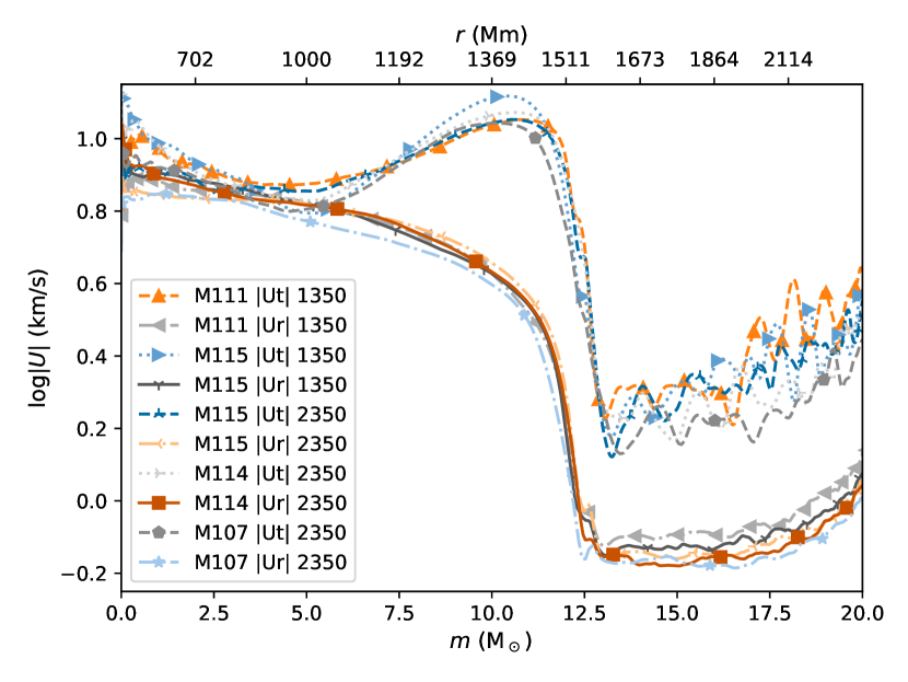
Figure 9: Spherically averaged radial and tangential velocity profiles for different resolutions (2688, 1728, 1152, 768, cf. Table 1). The legend provides simulation name, velocity component and time of profile in $\mathrm{\mathrm{h}}$.

As discussed in §3.1 the large-scale flow consists of a central radial column through the centre and a horizontal, arching return flow along the boundary. This general flow pattern is manifest in the spherically averaged tangential and radial velocity profiles (Fig. 9). In the centre of the core the radial and horizontal speeds are the same. Toward the boundary the radial velocity component decreases starting at a distance of about one pressure scale height. The horizontal velocity component however increases toward the boundary and peaks just below the convection boundary. This represents the comparatively fast boundary-layer flow. Inspection of the flow images (Fig. 3 and Paper I) shows that the boundary-layer flow separation typically starts around $3/4$ of the way from one end of the dipole to the other, (or $3/8$ of the circumference).

From these flow observations we estimate convective frequencies. In Paper I we have estimated a convective time scale adopting an average convective velocity of $U_{\mathrm{conv}}\approx 6.5\;\mathrm{km/\mathrm{s}}$ and as a distance the diameter of the convective dipole $2R_{\mathrm{conv}}$ which is $\approx 3000\;\mathrm{\mathrm{M}\mathrm{m}}$ with $R_{\mathrm{conv}}\approx 1500\;\mathrm{\mathrm{M}\mathrm{m}}$. This implies a convective time scale of $128.2\;\mathrm{\mathrm{h}}$, or a frequency of $2.17\;\mathrm{\mathrm{\mu{}Hz}}$. Alternatively one can consider the circular boundary-layer flow that returns material from where the radial flow impinges on the boundary to the antipode where the inflow forms. Considering that the excitation of waves is in part related to this boundary-layer flow one may adopt as a length scale the portion of the flow from where the radial outward-directed flow reaches the convective boundary and turns around to the location where the boundary flow separates as $3/4$ of $1/2$ of the circumference, which is $\frac{3}{4}\pi R_{\mathrm{conv}}$. The horizontal velocity magnitude near the convective boundary is higher ($U_{\mathrm{t}}\approx 10\;\mathrm{\mathrm{k}\mathrm{m}/\mathrm{s}}$) than the average radial velocity (Fig. 9). The convective time scale according to this adopted length scale and velocity is $T_{\mathrm{conv}}=98.2\;\mathrm{\mathrm{h}}$ corresponding to a frequency of $2.83\;\mathrm{\mathrm{\mu{}Hz}}$.

This exercise demonstrates that reasonably defined characteristic convective frequencies are in the same range as the prominent features of the low-frequency excess. The direct relation between these needs to be further investigated through a heating series of 3D simulations with the same radial stratification but different driving luminosities. Simulations at 10 times lower driving have $10^{1/3}$ times smaller velocities and therefore a characteristic convective frequency that is smaller by the same factor. The convective frequency at nominal ($1000\times$ smaller) luminosity is then $\approx 0.25\;\mathrm{\mathrm{\mu{}Hz}}$. Accordingly, if the prominent system of features evident in the spectrum of these simulations are directly reflective of the convective velocity they should be found at correspondingly lower frequency in simulations with lower driving luminosity. Demonstrating this effect requires very high frequency resolution and therefore very long runs. Such an analysis of the heating dependence of asteroseismic simulation properties (as in Le Saux et al., 2022; Blouin et al., 2022) is beyond the scope of this paper. However, spatial spectra for simulations with different heating factors discussed in §3.5 provide partial answers.

3.3 The nature of the oscillations in the stable envelope

Up to this point we have documented the stochastic properties of the luminosity oscillations and their correlation with velocity oscillations. We have established the presence of standing waves with stochastically variable amplitude. In order to further characterize the nature of these waves, and in order to determine the origin of the low-frequency excess of the luminosity spectra at a given radius of our simulation we construct frequency-wavenumber $l-\nu$ diagrams as in Herwig et al. (2006) where it was demonstrated how these diagrams allow the identification of IGWs and p modes as a function of radius when transitioning from the convection zone to the stable layer. However, first we determine the eigenmodes of the spherically-averaged radial stratification of the 3D simulations in order to place the $l-\nu$ diagrams from 3D simulations into context.

3.3.1 Predicted modes from GYRE

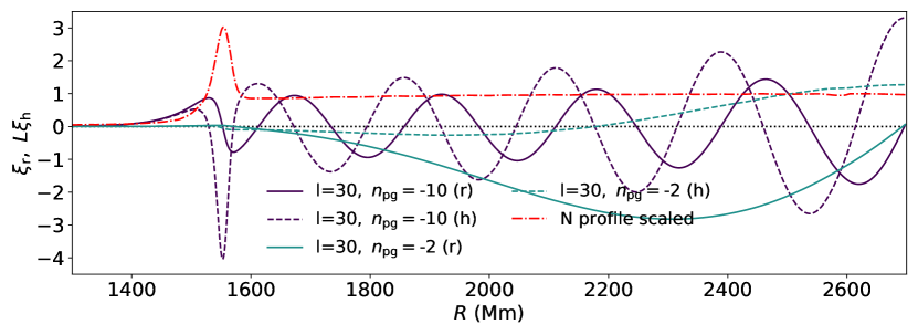
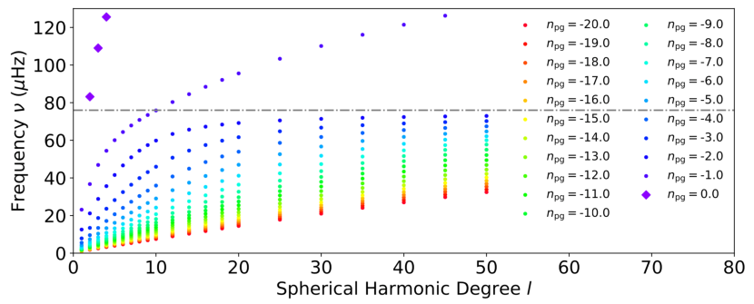
Figure 10: Top panel: Waveforms in terms of the radial $\xi_{r}$ and horizontal $L\xi_{\mathrm{h}}=\sqrt{l(l+1)}\xi_{\mathrm{h}}$ oscillation displacement amplitudes calculated using GYRE on spherically averaged radial profiles of simulation M114 at $116\;\mathrm{\mathrm{d}}$ for g modes with $l=30$ and $n=-2,-10$. The Brunt–Väisälä frequency is shown in red to indicate the location of the convective boundary region in which the $n=-1$ modes resonate (Paper I). Bottom panel: $l-\nu$ diagram calculated with GYRE for the same radial profile from run M114. The grey dash-dotted line shows the Brunt–Väisälä frequency representative for the envelope (Fig. 1). $n_{\mathrm{pg}}<0$ represent g modes. Low $l$ f modes for $n_{\mathrm{pg}}=0$ appear as well. p modes with low $l$ have frequencies larger than shown in this plot.

Usually GYRE is used to determine eigenmodes of a structure calculated by a stellar evolution code, such as the MESA code. Instead we use the spherically-averaged radial profile of a dump in the middle of the range used for the Fourier analysis of the 3D simulation M114 as input for the GYRE code. This allows us to identify the eigenmodes we expect in the 3D simulation (§2.4).

Fig. 10 shows the GYRE results (cf.  Pedersen et al., 2018, Fig. 2). In Paper I we have already discussed the role of the $n=-1$ g mode that dominates the $u_{\mathrm{r}}$ power in the narrow region of the $N^{2}$ peak where its prominent wave motions are clearly distinguishable in the velocity image renderings (Fig.  18, Paper I). Here we show the waveforms of some higher-radial order modes that have their largest amplitudes in the stable envelope above the convective boundary region. By identifying systematically the frequencies and $l$ for $-20\leq n\leq-1$ we arrive at the $l-\nu$ diagram schematic of eigenmodes shown in the bottom panel of Fig. 10. As expected g modes have frequencies in the envelope up to the Brunt–Väisälä frequency. For each radial order $n$ we obtain the arc-shaped dispersion relation that is characteristic of g modes.

GYRE can tell us $\nu$ and $l$ for each eigenmode with radial order $n$, but not how much power is in each of these eigenmodes. This information is of course contained in the output of our 3D simulation, and we will extract it in the next section.

3.3.2 $l-\nu$ diagram from the 3D simulations

The $l-\nu$ diagrams extracted from the 3D simulations are based on the last 2000 dumps ($\approx 1300\mathrm{hrs}$) of the $1152^{3}$-grid run M114. We choose to analyse a subset just long enough to achieve sufficient frequency resolution while limiting blurring the dispersion relations due to the slow evolution of the boundary in our simulations (Fig. 1 and Paper I).

In Fig. 11, we present diagrams from six mass coordinates from inside the convection zone and near convective boundary as well as from several locations in the stable envelope.

The power by mass coordinate and frequency is also plotted separately for 21 individual $l$ values in Fig. 12.

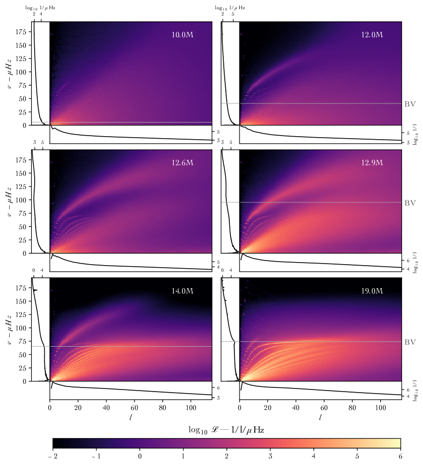
Figure 11: Oscillation power spectral density of relative luminosity decomposed by both frequency and spherical harmonic for run M114. The variable $\mathcal{L}$ is the power spectral density of the unity-subtracted, relative luminosity. The six panels correspond to different mass coordinates. Frequency in $\mathrm{\mu{}Hz}$ is plotted along the vertical axis, spherical harmonic degree $l$ along the horizontal, and power is represented logarithmically by the colour scale. The plots along the margins show the sum of the power along each axis. The horizontal line indicated by BV gives the Brunt–Väisälä frequency at that mass coordinate. Beginning from top left: at $10.0\;\mathrm{\mathrm{M}_{\odot}}$ the power inside the core is smooth and characteristic of turbulence, with few distinct features. At $12.0\;\mathrm{\mathrm{M}_{\odot}}$ which is inside the convection zone just below the convective boundary, the spectrum begins to show low order g modes couple to the convection. By $12.6\;\mathrm{\mathrm{M}_{\odot}}$, much more of the oscillation power is in a high $l$ mode confined to the boundary. By approximately $14.0\;\mathrm{\mathrm{M}_{\odot}}$ a full spectrum of g modes are excited and the spectrum (vs. frequency and vs. wavenumber) appears flatter out to the local Brunt–Väisälä frequency and $l\approx 60$. Further out in the envelope such as $19.0\;\mathrm{\mathrm{M}_{\odot}}$, the dominant mode from the boundary has died out at high $l$ as it exceeds the local Brunt–Väisälä frequency. We cropped the diagrams to only show lower frequencies and $l$ values where there is significant power and where we expect g modes.

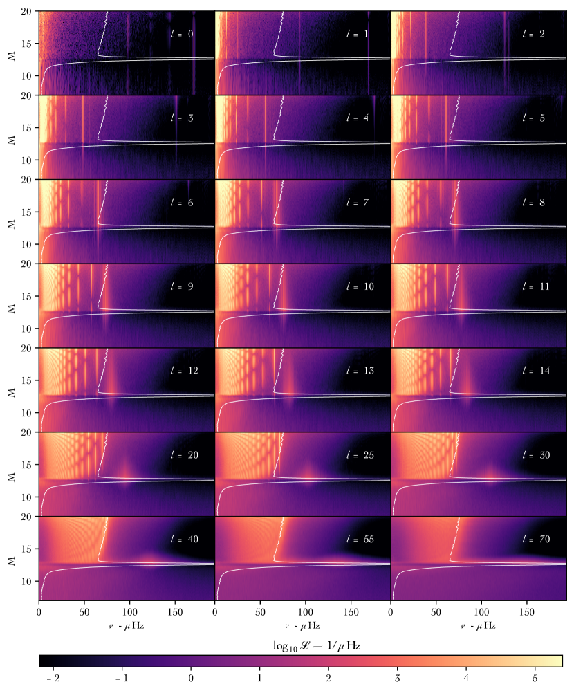
Figure 12: The relative luminosity power spectrum of M114 as a function of mass, separated by degree $l$. The variable $\mathcal{L}$ is the power spectral density of the unity-subtracted, relative luminosity. The turbulence visible throughout the core flattens as it approaches the convective boundary at approximately $12.5\;\mathrm{\mathrm{M}_{\odot}}$. At this point, a forest of g modes are excited in the envelope with frequencies approaching the maximum Brunt–Väisälä frequency of the envelope. The frequency and number of nodes along these vertical lines depend on their radial orders $n$, which are related to their angle of propagation through the envelope. The $n=-1$ boundary waves are visible above $f\approx 60$ peaking inside the narrow boundary region outlined by the Brunt–Väisälä profile in white. g modes cannot exist with $l=0$, so by process of elimination, the modes visible in the top-left panel must be f or p modes, which are not considered in this paper.

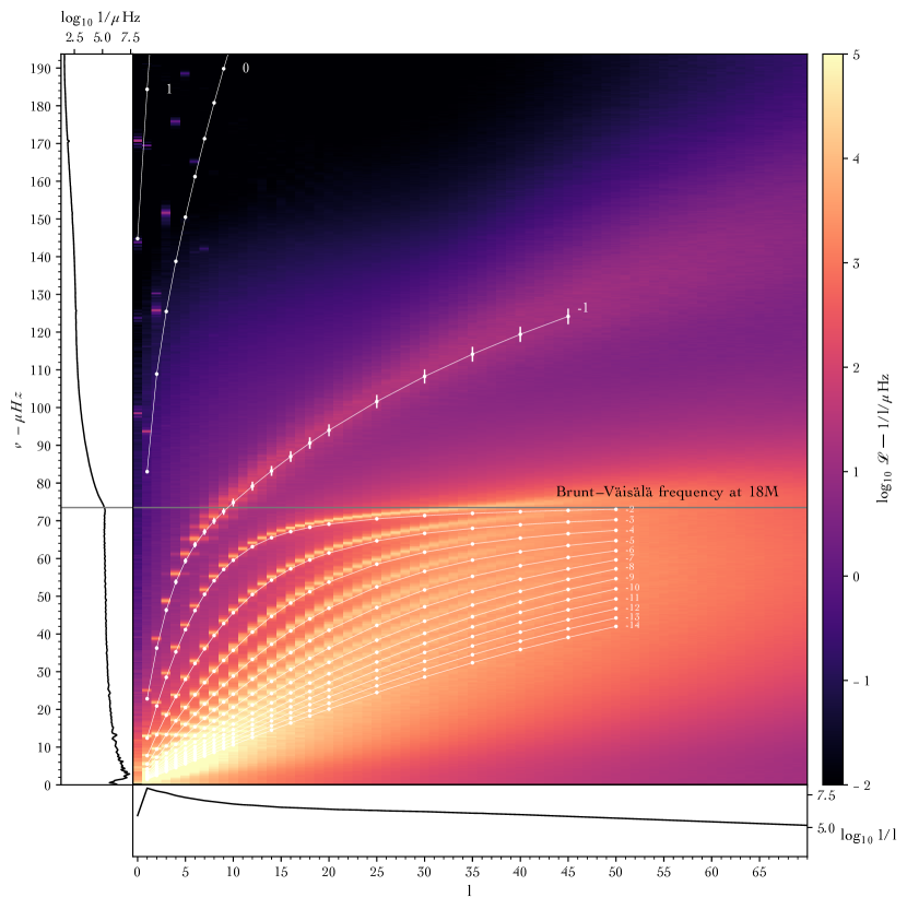
Figure 13: Frequency-wavenumber diagram averaged radially from the convective boundary to the edge of the M114 simulation. The colorscale displays $\mathcal{L}$, the power spectral density of the unity-subtracted, relative luminosity. We over-plot the eigenmodes predicted by GYRE as white lines and label them by their radial order $\mathrm{n_{pg}}$ where positive indices indicate pressure modes, zero indicates the f mode, and negative indices indicate g modes. The predictions of GYRE agree with the results of our simulations. This figure has been cropped – the numerical resolution of the simulation grid permits modes up to $l\approx 1800$. The GYRE calculations were run against the start and end dumps of the time span used to create the diagram, and then averaged. When visible, the vertical white bars indicate half of the difference between those calculations. We do expect some aliased p modes to visible in top left of the plot.

In $l-\nu$ diagrams gravity waves follow dispersion relations that appear as arcs that asymptotically approach the local Brunt–Väisälä frequency (see §3.3.1 for the corresponding GYRE predictions). The dispersion relations are modified by the radial order $n$, which relates to the angle of propagation, with oscillations in low $n$ waves being nearly radial and in high $n$ waves with the same $l$ approaching horizontal.

Beginning in the core at $10.0\;\mathrm{\mathrm{M}_{\odot}}$, the convection and turbulence produce smooth spectra (Fig. 11). The projection onto the spherical-harmonic degree $l$ horizontal axis shows power to be culminating at the lowest $l$ values and frequencies without any particular structure. This is typical for the irregular, intermittent turbulent motions of convective flow and has been documented already for deep interior simulations of He-shell flash convection (Herwig et al., 2006, Fig. 23, panel $y=4.70\;\mathrm{\mathrm{M}\mathrm{m}}$ and $y=7.45\;\mathrm{\mathrm{M}\mathrm{m}}$), for O-shell convection (although less clearly Meakin & Arnett, 2007, Fig. 7, middle panel) as well as core convection (Rogers et al., 2013). The accumulation of power in the convective region at low frequencies and low wave numbers reflects the nature of the turbulent spectrum of convection (e.g. Fig. 6, Paper I) and is most clearly displayed for radii sufficiently deep inside and distant from the convective boundary. The power in the lowest frequency bins of a few $\mathrm{\mu{}Hz}$ relates to the convective frequency (§3.2.4). However, at $10.0\;\mathrm{\mathrm{M}_{\odot}}$ which is approximately one pressure scale height below the convective boundary (Fig. 9), a faint signature emerges of the ordered arc-like pattern of power distribution associated with IGWs appears. This arc belongs to the $n=-1$ modes that have their largest displacement amplitude near the convective boundary.

Stepping outward, the general pattern is that power redistributes into different sets of IGW eigenmodes. The mass coordinate $12.0\;\mathrm{\mathrm{M}_{\odot}}$ is close to the convective boundary on the unstable side. The distribution of power shifts to a flatter $l$ spectrum. The arcs of the lowest radial order $n$ IGWs now contain more power. The $l-\nu$ diagram at this mass coordinate shows a mix of the unordered convective power distribution and the regular patterns reminiscent of IGWs. Thus, in the outermost layers of the convection zone motions are due to a mix of IGWs and turbulent convection. This gradual transition from convection-dominated to IGW-dominated flow fields is documented in Paper I. At $12.6\;\mathrm{\mathrm{M}_{\odot}}$ we arrive at the peak of the Brunt–Väisälä frequency profile. Here, the power in the region at low $l$ and $\nu$ which dominated inside the convection zone is momentarily diminished, demonstrating that irregular, turbulent convective motions generally do not reach this radial location. It also shows that at and above the $N^{2}$-peak radius, motions are dominated by IGWs and not, for example, by plume overshooting.

In Paper I we showed that the radial location of the $N^{2}$ peak is an important separation line between the convection-dominated flow below and the IGW wave dominated flow above. In this region of the $N^{2}$ peak significant power is present in the $n=-1$ g modes with a large range of $l\lessapprox 80$ (cf. Fig.  19, Paper I). Higher order g modes exist but have insignificant power. The power spectrum has now completely changed, peaking at $l\approx 70$ and $\nu\approx 140\;\mathrm{\mathrm{\mu{}Hz}}$. The dominant presence of the $n=-1$ mode depends on the exact shape of the $N^{2}$ profile, something that 3D hydrodynamic simulations aim to ultimately determine. This shape is a combination of hydrodynamic and secular time scale processes (Paper I). If real stars feature a prominent $N^{2}$ peak at the convective boundary the $n=-1$ IGW clearly plays a key role in the physics of convective boundary mixing.

The boundary region ends at approximately $12.9\;\mathrm{\mathrm{M}_{\odot}}$ where the $N^{2}$ profile reaches a local minimum. At this radius power shifts to IGW modes that oscillate predominantly in the envelope with $n\leq-2$ at lower frequencies, below the local Brunt–Väisälä frequency, and lower $l$. This general trend continues for larger radii. At $14.0\;\mathrm{\mathrm{M}_{\odot}}$, some distance from the boundary region and the bottom region of the stable envelope, the power in the high $l$, $n=-1$ boundary waves is greatly diminished as they now exceed the local Brunt–Väisälä frequency. The spatial power spectrum peaks at low $l$ but has significant power out to $l\approx 80$ thanks to a large population of modes with a wide range of $l$ and $n\leq-2$. At this point, the spectrum reaches a turning point at frequencies just below the BV frequency with a sharp drop of power beyond.

At the largest mass coordinate shown, the power in the $n=-1$ boundary mode has vanished. Essentially all power is in IGW modes with $n\leq-2$. A full range of g modes are excited for many $n$ and $l$ values exceeding 100. A key feature of the frequency spectrum summed up for all $l$ shown on the horizontal axis of each panel, is the large amount of power near the BV frequency. This power originates from high-$l$ and relatively low-radial order g modes. It becomes clear that in order to understand the low-frequency excess shown in Fig. 8 the substantial contributions of moderate-$l$, and high-radial order $n$ IGW modes near the BV frequency is key.

When interpreting the $l-\nu$ diagram panels for mass coordinates in the stable layer, one needs to keep in mind that the $l-\nu$ diagrams do not show any power where a mode has a radial node, and thus some modes along the regular arcs are not seen very strongly. This is clearly seen for example for the $n=-4$ g modes for the $19\;\mathrm{\mathrm{M}_{\odot}}$ panel in Fig. 11 and in Fig. 12 where the radial power distribution is shown as function of frequency separately for 21 $l$ values. In that diagram each vertical line in the stable layer corresponds to one radial order $n$, and the dark gaps in these vertical lines correspond to nodes. The frequency of the vertical line for each order $n$ increases from panel to panel with $l$, tracing out the dispersion relation arcs from Fig. 11.

It is worth noting that these modes are not sharp and have line widths much greater than we would expect from the Hanning window function applied to control spectral leakage. Some of this broadening comes from evolution of the Brunt–Väisälä profile throughout the simulation as can been seen in the white error bars of Fig. 13; however, the more significant contributor to the line width of these modes is their finite coherence, since the modes are driven stochastically and have a finite lifetime.

Before discussing the coherence of these modes below, we return briefly to the interpretation of Fig. 6 now that we have established that the waves are indeed IGW. The power at each frequency usually does not correspond to an individual IGW mode, but rather to a superposition of modes with different radial order $n$ and spherical harmonic degree $l$ as shown in §3.3.1. However, in order for the power to vary over time, the contributing modes must be variable. Thus, the variability of mode amplitudes as the result of their stochastic excitation by the underlying core convection is also evident from the sliding spectral representation of Fig. 6.

3.3.3 Internal gravity waves in the stable envelope

The general features of the power distribution in the $l-\nu$ diagrams shown in Fig. 11 show a close resemblance of the eigenmodes calculated by GYRE shown in Fig. 10. In fact, we can extend the comparison with the modes as shown in Fig. 12 to include the GYRE information. In the top panel of Fig. 10 the waveforms are shown for $n=-2,-10$ and spherical harmonic degree $l=30$. The solid lines gives the displacement amplitude for the radial velocity component and dashed lines give the horizontal displacement amplitude.

Comparing the GYRE calculations in Fig. 10 to the 3D simulations in Figs. 11 and 12, we can directly identify the individual eigenmodes at the correct frequencies and see that their power evolves with radius as expected.

Extending this comparison to many modes, Fig. 11 overlays eigenmodes calculated by GYRE from the spherically averaged radial profile to the a $l-\nu$ diagram of the 3D simulation, averaged radially across the envelope. The radial averaging avoids missing modes that have nodes at some radii. The GYRE g mode predictions and the results of the 3D simulation agree very well across the whole range of $l$ and $n$. This shows that fluid motions in the envelope are indeed predominantly IGWs. The f mode indicated by $n=0$ and first two p modes are also present but with frequencies approximately 20 percent higher frequency than calculated by GYRE.

The frequencies predicted by GYRE agree within at most 7 percent relative error for high-$l$ g modes with the frequencies of eigenmodes in the PPMstar simulation. In Fig. 13 we show the frequency difference of GYRE predictions based on the spherically averaged radial profiles of two dumps, one near the beginning of the sequence analyzed to create the $l-\nu$ diagrams, and one near the end. This shows that according to the GYRE prediction the small change in the profile contributes little to the broadening of the lines for all but the $n=-1$ modes.

3.3.4 Coherence time of modes

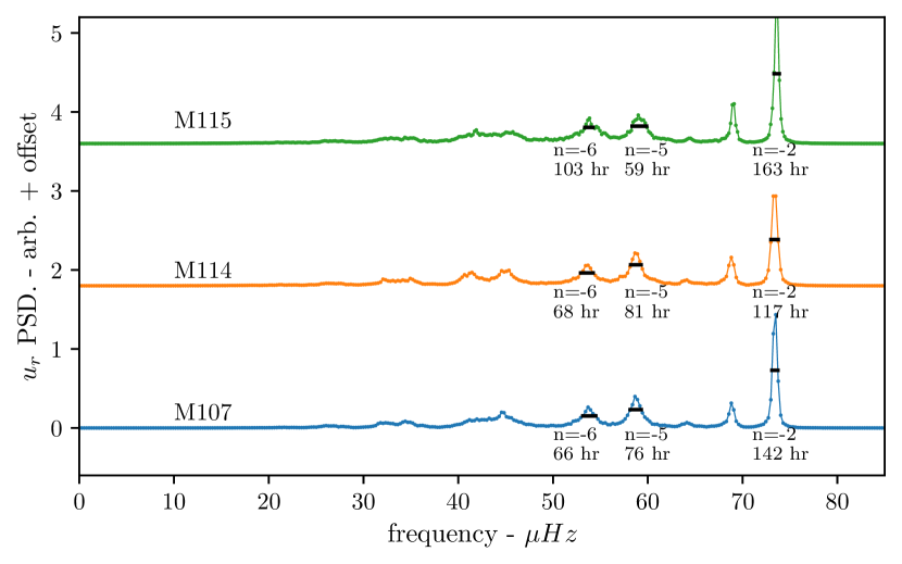
Figure 14: Coherence times measured from three modes at $l=30$ and a mass coordinate of $19\mathrm{M}_{\odot}$ for three different grid sizes. There is no clear trend in coherence time with grid resolution, and considerable variation between $n$ and $l$ mode numbers. The relatively short coherence times are a result of the stochastic excitation by convection in the core.

As visible in Fig. 6, we find that the standing g modes in the envelope vary in power considerably over time. To evaluate the coherence of these g modes, we measure the full width at half maximum of a few characteristic peaks in the M114 $l-\nu$ diagram in Fig. 14. The full width at half maximum $2\Delta\nu$ of a mode that is not otherwise broadened by other effects is directly related to the coherence time by the relation $1/(2\Delta\nu)$. For low-$n$ g modes of order $l=30$, we find coherence times in the range of 80-100 h. We attribute this limited coherence and short lifetimes to the stochastic nature of the excitation and re-excitation from core convection (cf. discussion at the end of §3.2.2).

3.4 Origin of the low-frequency excess

We are now equipped to describe the origin of the low-frequency excess (Fig. 8) described in §3.2.3. By doing so we reconsider two points that could be raised as possible challenges for a low-frequency excess having the general shape of the one shown in Fig. 8 to originate from excitation through core convection (e.g. Lecoanet et al., 2019a). One is that the core convection excitation is limited to low $l$ and the other related point is that higher-$l$ modes would cancel in the hemispheric integration. A third important point is the effect of radiation that we do not include in this paper (see §4).

3.4.1 The excitation spectrum

A key result from our high-resolution 3D core-convection simulation is a detailed characterization of the dynamic motions near and across the convective boundary (see Paper I for additional details). As concluded in §3.3.4, wave energy is also returned to the convective core to arrive at an equilibrium between excitation and de-excitation. For this reason, it might be better to describe this as the equilibrium spectrum. Regardless of the name, a simple picture of convection motivated by mixing-length theory would suggest that the dominant power resides in the lowest $l$ modes (representing the mixing-length blob rising for the distance of a mixing length). While we do see that power peaks at low $l$ modes, significant power is nonetheless present up to much higher $l$ as well.

We showed in Paper I (Fig. 6) that the spectrum of the radial velocity flattens significantly near the convective boundary compared to the regions deep inside the convective core and compared to the tangential velocity. This is simply a result of the low-$\mathcal{M}$ Mach number and therefore essentially incompressible flow changing from predominantly radial to predominantly horizontal near the convective boundary (Fig. 9). This flattening of the spatial spectrum near the convective boundary is a general feature of interior convection and has also been documented for He-shell flash convection in rapidly accreting white dwarfs (Stephens et al., 2021).

The motions contributing to power at large $l$ are physically associated with the boundary-layer separation wedges (§3.1, Paper I). Thus, at the convective boundary a broad spectrum of scales and frequencies with power at small and large $l$ are present that couple to and inject energy into the IGW modes of the stable envelope. Finally, Fig. 12 reveals that it is not strictly necessary to have as much power at a given $\nu$ and $l$ at the convection boundary as in an excited IGW in the stable layer.

3.4.2 Attenuation

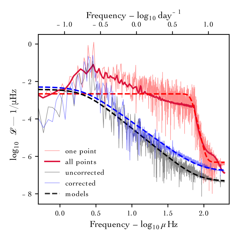
Figure 15: Luminosity spectra extracted at $19.5\;\mathrm{\mathrm{M}_{\odot}}$ from our M107 simulation in three different ways. The “one point” spectrum is measured at just a single point on the sphere. The uncorrected spectrum is integrated uniformly over one hemisphere. The corrected spectrum integrated over hemisphere and corrected for Lambert’s cosine factor $\cos(\theta)$, converting the surface integral into an integral over the projected disk of the star. The integrated luminosity power spectra are attenuated significantly where the spectrum is dominated by higher $l$ modes. The latter method is used throughout this paper. The all points spectrum is similar to the one point spectrum, but is instead extracted from a frequency-wavenumber diagram of M114 (left margin panel of Fig. 13). This is similar to averaging one point spectra across a surface of the sphere.

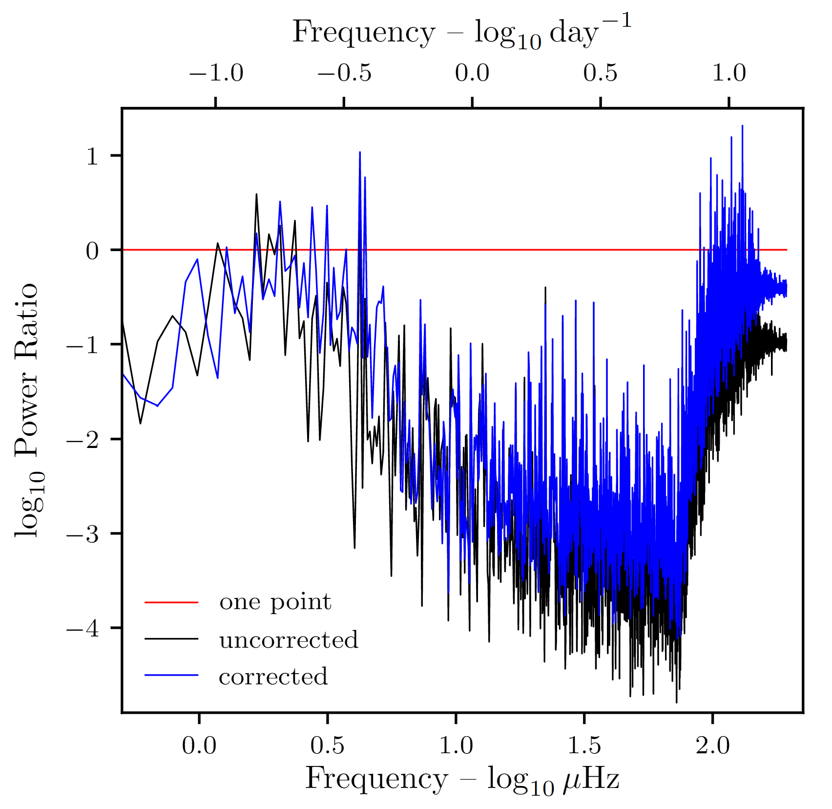
Figure 16: The attenuation of the luminosity power spectrum when integrated across one face of the simulation, compared to a spectrum extracted from a single point (integrated power spectra divided by the single point spectrum). The strongest attenuation occurs where the spectrum is dominated by higher $l$ modes.

Through the analysis of the $l-\nu$ diagrams presented in the previous section we have established that the fluid motions in the envelope are IGWs and that the substantial power contribution to frequencies just below the Brunt–Väisälä frequency originates from the superposition of modes with the approximate range of spherical harmonic degree $15\lessapprox l\lessapprox 40$ and with small radial orders in the range $-6\lessapprox n\leq-2$. While the highest power lies in individual modes with low $l$ and $\nu$, the combined power from the superposition of waves with a wide range of higher $l$ contributes significant power out near the Brunt–Väisälä frequency. Radial order $-5\leq n\leq-2$ and $l\approx 30$ modes are responsible for the power in the upper half of the frequency range up to the BV frequency.

We now consider how different approaches of turning the 3D wave field into a simulated light curve impact the resulting synthetic spectrum. We consider three options. The first is to take the luminosity only at one point on a 3D sphere of a given radius, somewhat similar to Edelmann et al. (2019b) who used eight points. We refer to this in Figs. 15 and 16 as one point. The second is to integrate at each dump over a hemisphere of the simulated star at a given radius and into the direction of a given line-of-sight (§2.2) to obtain time series of single luminosity values. Finally, we consider the correction due to Lambert’s cosine factor as described in §2.2. The latter two options are referred to as uncorrected and corrected respectively. The spectra generated using these three options are compared in Fig. 15. A tentative fit of a Lorentzian model to the one point spectrum places $\nu_{\mathrm{char}}\approx 3.8\;\mathrm{\mathrm{d}}^{-1}$ close to the BV frequency of this model, and much higher than the value determined for the spectrum according to the corrected approach reported in §3.2.3. The one point spectrum has a pronounced flat low-frequency plateau with a relatively gentle slope from the peak near the convective frequency toward the envelope BV frequency.

That said, a photometric observation receives light that is the 2D integration over the projected face of a hemisphere. This integration cancels luminosity peaks and troughs of oscillations. The cancellation is expected to be largest for high-$l$ modes, and for coherent oscillations only the partial peaks and troughs along the rim that have no exact counterpart are expected to contribute net flux to the oscillation. This rim contribution is further diminished by applying the $\cos(\theta)$ Lambertian projection factor (§2.2). These are all good reasons to expect that high-$l$ modes do not contribute significantly to spectra over an entire hemisphere. However, our simulations suggest otherwise.

The uncorrected spectrum in Fig. 15 also shows the spectrum of the same simulation, but integrated over a full hemisphere. The cancellation effect of the integration is clearly present, and it attenuates power from the higher frequency range below the BV frequency that is associated with high-$l$ modes (as explained in the previous section). Performing a Lorentzian model fit results in a substantially lower parameter $\nu_{\mathrm{char}}$ (which identifies the edge of the low-frequency plateau) and a smaller parameter $\gamma$ (that describes the slope from the red noise to the level of the white noise). However, the power is not attenuated completely and, at least in the simulation, we still detect power out to the BV frequency, Thus, the hemispheric integration indeed cancels high-$l$, but not to the level that they become entirely insignificant.

Applying the $\cos(\theta)$ correction further reduces $\nu_{\mathrm{char}}$, though the additional effect is relatively small. This can also be seen in Fig. 16 where we show again the spectra for all three cases as well as their ratios. Power at high $l$ is largely present at intermediate frequencies approaching the BV frequency of the envelope (see Fig. 11). Accordingly, the attenuation between considering just one point on the equator and integrating over one face of the simulation is strongest between frequencies of 1 and 10 $\mathrm{\mathrm{d}}^{-1}$. Applying the $\cos{\theta}$ correction does not effect the cancellation significantly.

This suggests that the oscillation contributions escaping cancellation do not primarily come from the rim, but that instead cancellation effects are smaller than one may expect because the oscillations are stochastic (Fig. 5,§3.2.2, 3.4). Especially stochasticity in phase would reduce cancellation effects compared to the case of coherent oscillations. In fact, we have seen in Fig. 4 that the luminosity oscillations have fluctuations in different directions of the same hemisphere with different phases.

This leads to a key result. A power spectrum such as the one shown in Fig. 8 is the result of attenuation through hemispheric integration of high-$l$ modes of an underlying spectrum relatively flat for $\nu<\nu_{\mathrm{BV}}$. The attenuation does not entirely suppress the modes with frequencies closer to the BV frequency. Instead, the slope of the decrease of power from the red noise level at $\nu_{\mathrm{char}}$ to the intercept of white and red noise changes by the cancellation due to hemispheric integration. This slope is expressed in terms of the parameter $\gamma$ of the Lorentzian model fit. It in turn depends on the power distribution in terms of $l$ and $\nu$ and on the stochastic nature of the excitation, as we believe this reduces the cancellation compared to the case of coherent oscillations.

Finally, we note that the low-frequency power excess falls to the level of the white noise at the BV frequency. In other words, the location where the red noise intercepts the white noise indicates the peak BV frequency in the envelope, assuming that no other observational white noise sources dominate. This frequency $\nu_{0}$ changes less than $\nu_{\mathrm{char}}$ when integrating over the hemisphere with and without Lambertian correction factor.

3.5 Convergence and dependence on heating factor

For results of any 3D hydrodynamic simulation an important question is always to what extent the finite grid resolution affects the results in question. This is especially true in light of conflicting results between simulations, and how those results depend on luminosity and resolution (Lecoanet & Edelmann, 2023).

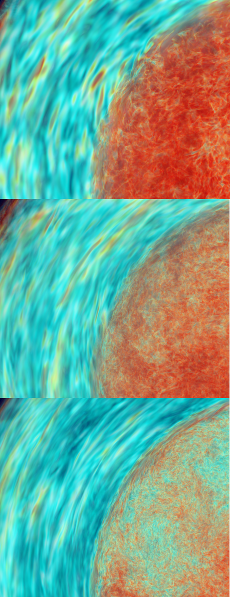
Figure 17: Zoom-in vorticity images (center plane) for dump 2150 ($1540\;\mathrm{\mathrm{h}}$) for simulations M107 ($768^{3}$), M114 ($1152^{3}$) and M115 ($1728^{3}$), from top to bottom.

Fig. 17 shows vorticity images for a zoomed-in region of the simulation for three different grid resolutions taken from the same time step. The overall morphology of the flow is similar for all three resolutions and as expected higher resolution simulations show more small-scale structure.

This is reflected in the spatial power spectra of the velocity magnitude shown in Fig. 18 for simulations with grids from $768^{3}$ to $2688^{3}$. Note that spatial spectra velocity magnitude are essentially identical to luminosity spectra which were for technical reasons not available for all simulations shown in Fig. 18. As expected, simulations with higher resolution contain power at increasingly higher spherical harmonic degree $l$. Considering the dispersion relation of IGWs (Fig. 13) high-$l$ power is associated with higher frequencies where most of the attenuation takes place (§3.4.2). This de-emphasizes the already small impact of grid resolution on the frequency spectra since geometric attenuation is most effective at high $l$. At lower $l$ the agreement between simulations with grids of $1152^{3}$ and higher is very good. Importantly, the shape of the spectrum depends little on grid resolution.

The temporal spectra for the same set of grid resolutions is shown in the top panel of Fig. 19. These have been obtained based on the time series shown in Fig. 20. As can be expected higher resolution runs are shorter. This impacts the frequency resolution. However all simulations are long enough to capture the peak of the power spectral density at $\approx 2.7\;\mathrm{\mathrm{\mu{}Hz}}$, essentially the same as the convective frequency (§3.2.4). We exclude as before the initial transition period (§3.2.1) and compared to spectra shown in §3.2.3 we are using for this comparison the same (smaller) radius as for the spatial spectra (Fig. 18). The good agreement between spatial and temporal spectra for the four resolution simulations spanning overall a grid size factor of $3.5$ as well as the absence of an obvious trend of the mode life times reported in Fig. 14 suggests that numerical effects commonly associated with insufficient numerical resolution are not impacting our results.

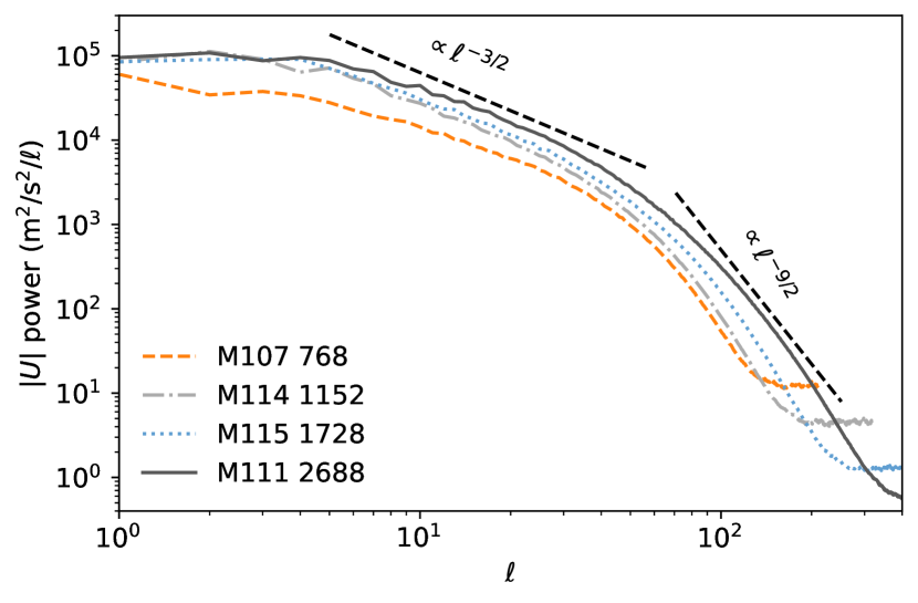
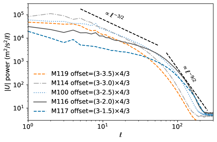
Figure 18: Spatial power spectra of velocity magnitude at radius $1900\;\mathrm{\mathrm{M}\mathrm{m}}$. Each line is the average of hundreds of dumps to remove short-term spectral variations. Top: Simulations with $1000\times$ ($10^{3}$) heating factor for different grid resolutions as indicated in the legend. Bottom: Spectra for different heating factors from $1152^{3}$-grid simulations (table 1, Paper I) as indicated in the legend. The heating factor for each case is given as the log heating rate subtracted from $3$ as given in the bracket in the legend. For example, the heating factor simulation M119 is $10^{3.5}$. Each heating run has been shifted according to the scaling $u_{\mathrm{IGW}}\propto L^{2/3}$, see section 5.2 in Paper I. Power laws have been added with dashed lines to guide the eye. Simulations shown that are not included in Table 1 are discussed in detail in Paper I.

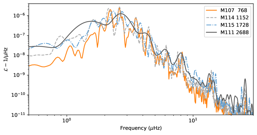
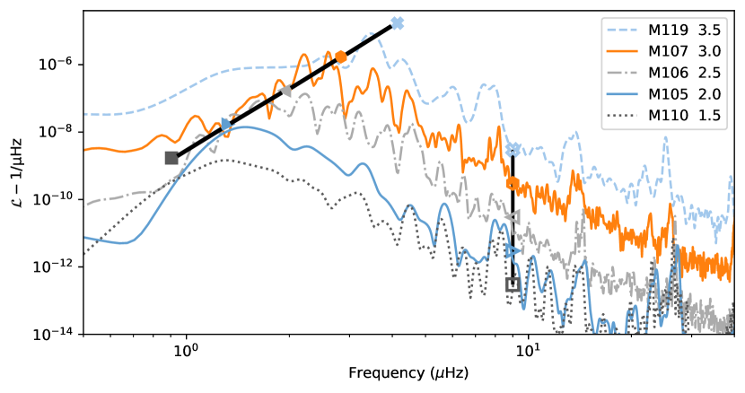
Figure 19: Temporal power spectral density of the unity-subtracted, relative, hemispherically integated luminosities $\mathcal{L}$, averaged over all eight lines-of-sight (§2.2), and using for each simulation the time series shown in Figs. 20 and 21 at radius $1900\;\mathrm{\mathrm{M}\mathrm{m}}$. Spectra have different frequency resolutions due to the different simulated time range available and/or adopted in the analysis. Top: Simulations with $1000\times$ heating factor for different grid resolutions as indicated in the legend. Bottom: Spectra for different log heating factors based on $768^{3}$-grid simulations, except M119 which is $1152^{3}$ grid. Filled markers are added at frequencies $\propto L^{1/3}$ reflecting the scaling of the convective frequency. The vertical position of the markers is $\propto L^{2}$ and the offset is chosen to approximately match the power of simulation M107. A second set of open markers connected with a vertical line is added at $9\;\mathrm{\mathrm{\mu{}Hz}}$ with the same heating factor scaling. Simulations shown that are not included in Table 1 are discussed in detail in Paper I.

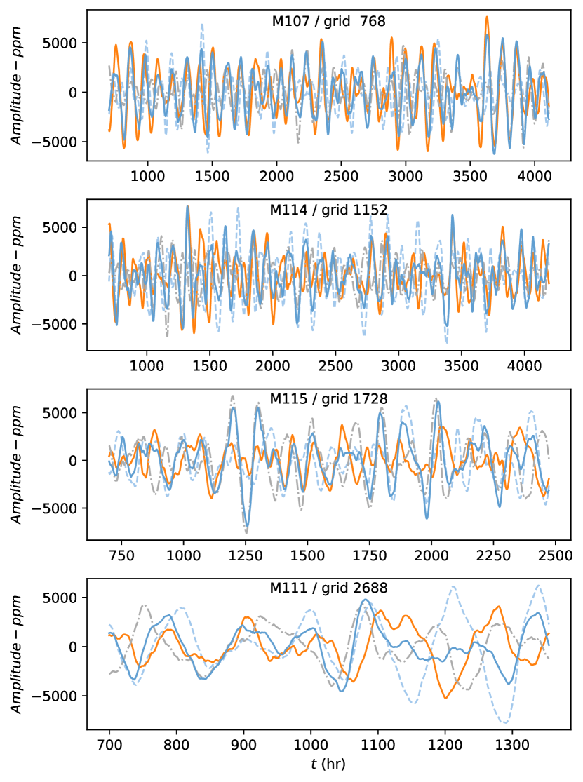
Figure 20: Time series of first four line-of-sight hemispherically integrated luminosities at radius $1900\;\mathrm{\mathrm{M}\mathrm{m}}$ for the resolution series used for the temporal spectra shown in Fig. 19. The text label gives the simulation name and the grid size.

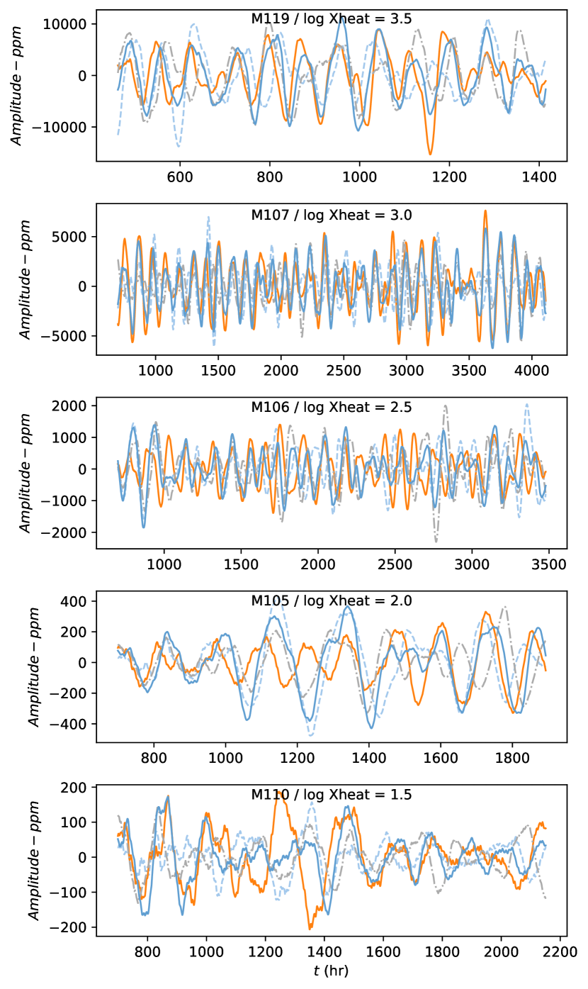
Figure 21: Time series of first for line-of-sight hemispherically integrated luminosities at radius $1900\;\mathrm{\mathrm{M}\mathrm{m}}$ used for the heating series temporal spectra shown in Fig. 19. The text label gives the simulation name and the log of the heating factor.

The dependence of IGW spectra driving luminosity deserves attention as well since all of our simulations are at a considerable boost factor. Demonstrating that spectra are self-similar not only under grid refinement but also as a function of heating factor is key for extrapolating from boosted simulations to nominal heating. We have already shown in Paper I (section 5.2) that for heating rate factors $\leq 100$ for an $1152^{3}$ grid and $\leq 316$ for a $752^{3}$ flow velocities start to depart from scaling relations, thereby indicating decreasing levels of accuracy. Figs. 18 and 19 show both spatial and temporal spectra as a function of heating factor. The two lowest heating-factor simulations show somewhat flatter spatial spectra that extend relatively to higher anglar degree $l$. The three higher heating rate simulations agree well with each other when scaled according to $U_{\mathrm{IGW}}\propto L^{2/3}$.

The temporal spectra are shown in the bottom panel of Fig. 19. The frequency-integrated power spectrum density $\int\mathcal{L}d\nu$ scales linearly with the heating factor, with a deviation from the linear fit of $-2.5$, $-6.8$, $7.5$, $20.4$ and $-14.2\%$ from low to high heating factor. Markers are positioned at the convective frequency corresponding to the respective heating factor with vertical shifts reflecting the just mentioned scaling. The peaks of the spectra evolve with heating factor with almost the same rate as the expected convective frequency. Such a correlation was recently reported by Le Saux et al. (2022). The same analysis at a larger radius of $2400\;\mathrm{\mathrm{M}\mathrm{m}}$ showed an even smaller relationship between spectrum peak frequency and heating factor.

A second set of open markers at $9\;\mathrm{\mathrm{\mu{}Hz}}$ reflects the scaling found for the integrated power spectral density, and indicates that this scaling applies not only approximately to the peak power but also at other frequencies. Overall it appears that the spectra are mostly self-similar with respect to heating factor.

4 Discussion

Based on 3D hydrodynamic simulations of a $25\;\mathrm{\mathrm{M}_{\odot}}$ star near the beginning of its main sequence evolution we have investigated the excitation and spectrum of IGWs in the stable layer excited by core convection. The key convection and convective boundary properties of these simulations have been reported in Paper I. The key results of this paper can be summarized as follows:

• Deep inside the convective core the flow is well represented by a fully-developed Kolmogorov power spectrum. However, near the convective boundary the flow is dominated by horizontal flow topologies, in particular the boundary-separation flow wedges (cf. Paper I) where unstable flow morphologies with a wide range of scales are generated.

• The broad range of scales of fluid motions near the boundary excites IGWs with a broad range of spherical harmonic degrees $l$ and radial order $n$. The power remains significant up to $l\approx 30$ and the dispersion relations for radial orders up to $n\approx-10$ can be clearly distinguished in the $l-\nu$ diagram. These agree with the GYRE predictions for the spherically averaged radial profile of the 3D simulation demonstrating that the oscillations are indeed IGWs.

• The $n=-1$ g modes populate the convective boundary region where due to the choice of our initial profile from a MESA stellar evolution model the profile of $N^{2}$ has a sharp peak (see Paper I for details).

• The power in different IGWs fluctuates stochastically. This may reduce the cancellation effect when integrating photometric variability due to IGWs over a hemisphere.

• IGWs have a broad distribution of power at moderate to high $l$ which corresponds, according to the dispersion relation of IGWs as seen in Fig. 13, to relatively high frequencies near the Brunt–Väisälä frequency. This power at high frequencies is attenuated by the cancellation in spherical integration, but not to the level of insignificance.

• The combination of these two effects—the excitation of high-$l$ IGWs and reduced attenuation of incoherent IGWs—leads to a spectrum (right panels in Fig. 4 and Original in Fig. 7) in which the power peaks in the frequency range that coincides with the convective frequency and then gradually tapers off toward the Brunt–Väisälä frequency.

• When further applying the same pre-whitening procedure as is applied to observational data (Bowman et al., 2019a, 2020) the low-frequency peaks that coincide with the convective frequency are removed resulting in a flat red noise spectrum shown in Figs. 7 and 8.

• Spatial and temporal spectra show little dependence on grid resolution. The temporal spectra show a clear trend of the peak frequency with heating factor, with almost the same power as the convective frequency. The overall shape of the spatial and temporal spectra is self-similar with respect to heating factor.

• Since the convective velocity scales with $\propto L^{1/3}$ the convective frequency at nominal heating would be 10 times lower (thus $\approx 0.27\;\mathrm{\mu\mathrm{Hz}}$) compared to our $1000\times$ simulation, and therefore challenging to access with current observations.

Our simulations do not include the effect of radiative damping (§3.2.2). Similar simulations to the ones analysed here have been presented in Paper III, where it has been shown that adding radiative diffusion does not alter the spectra enough to change the key findings of this work. Radiation diffusion is expected to happen predominantly near the surface which we do not include, and it may also damp low temporal frequencies more than higher ones (Zahn et al., 1997). How this damping manifests itself in the context of the other processes discussed here (e.g. §3.2.2) that lead to the formation of the IGW spectrum remains to be investigated. However, a key question is what role the IGWs excited by core convection play in generating the observed low-frequency excess in O and B stars. Lecoanet et al. (2019a) argue that the observed low-frequency excess cannot be due to IGW excitation from core convection, based on mainly two arguments relating to waves with $l\leq 3$. One key argument is that these low-$l$ waves should leave distinguishable features in the spectrum. Our simulations show that such individual features can be swamped in the forest of lines from the power residing at higher $l$ ($15\lessapprox l\lessapprox 45$). Lecoanet et al. (2019a) discard such high-$l$ waves in their analysis presumably because they correspond to frequencies much higher than the convective frequencies, and it is maybe assumed that such high $l$ and high $\nu$ modes cannot be excited. Our simulations show that such waves are efficiently excited in boundary-flow features such as the boundary-layer separation wedges. Omitting high-$l$ waves would also be justified due to the expected cancellation effect in hemispheric integration which our simulations show to not be completely efficient, likely due their stochastic nature. In our simulated, hemispherically integrated spectrum the Lorentzian downturn expressed in the parameter $\gamma$ represents indeed the high-$l$ wave power attenuated by incoherent IGW cancellation.

Although our simulations do not support the reasons for the suggestion of Lecoanet et al. (2019a) that the observed red noise in massive stars is not caused by convective core excitation, we do agree with the notion that IGWs excited by convective core convection alone may not fully account for the observed spectra, based on conventional massive star stellar structure such as those used as initial model for our simulations. The basic argument is that only the $n=-1$ mode produces power at frequencies larger than the Brunt–Väisälä, because it predominantly exists in the boundary region where the Brunt–Väisälä frequency is indeed larger. The $n=-1$ power is evanescent in the stable layer above, and at the mass coordinate $19\;\mathrm{\mathrm{M}_{\odot}}$ the Brunt–Väisälä frequencies at that mass coordinate is the expected and actual frequency limit above which power drops off significantly. When adding the hemispheric cancellation no power above the white noise remains in the simulated spectra. Thus, power at frequencies larger than the Brunt–Väisälä frequency in the stable layer above the core are efficiently filtered as expected, and cannot reach the surface. However, most observations of O and B stars have larger $\nu_{\mathrm{char}}$ than our Lorentzian fit (with or without pre-whitening). A quick survey of standard massive star evolution main-sequence tracks (Ritter et al., 2018) shows that the Brunt–Väisälä frequencies in these models in the region above the convective core is never large enough so that observed $\nu_{\mathrm{char}}$ can be populated. However, the Brunt–Väisälä frequency in the near-surface region is typically larger by a factor $\approx 8$ which generally reproduces the observed range of $\nu_{\mathrm{char}}$ values better.

It has been suggested that the FeCZ zone would excite waves in the surface region (Cantiello et al., 2009; Lecoanet et al., 2019b; Schultz et al., 2022). Our simulations do not provide arguments that would speak against that. However, the FeCZ is rather thin, with an aspect ratio of $\lessapprox 0.1$. It is not clear to us how low-$l$ IGWs can be excited by a convection zone that, due to its geometry, can only support coherent convective structures with large $l$. We therefore speculate that the observed low-frequency excess is excited by a combination of core convection and near-surface convection zones, where the former contribute power to the lower frequencies and the surface convection adds power to the higher-frequency range. We expect that the reduced attenuation of incoherent IGWs would also apply to hemispheric integration of high-$l$ modes excited by near-surface convection modes. Indeed, (Bowman et al., 2020) observe a trend in the inferred morphology of the low-frequency power excess between younger and older stars. Such a transition also argues for both convective regions contribute to the excitation of IGWs observable at the surface, with a relative contribution of the two mechanisms that depends on the structure (i.e. age) of the star (Bowman & Dorn-Wallenstein, 2022).

If the low frequency excess observed at the surface does indeed originate from IGWs in the envelope, then the shape of the low-frequency excess could provide direct measurements of certain properties of the core and envelope. For instance, we note that the location where the tail of the low-frequency excess falls to a negligible level coincides with the peak Brunt–Väisälä frequency of the envelope. Assuming that observational noise does not overwhelm this signal, it could be used as a direct measurement of the properties of a star’s envelope. In a similar vein, we showed that certain coherent modes above the IGW background are variable. Individual modes can be seen in a spectrogram (Fig. 6) to vary in power during the simulation, and in some cases disappear before being stochastically re-excited. If this is detected in observations, properties like the mean lifetime of these modes or time scale after which they are re-excited could probe the core convection. Indeed, the sliding Fourier transforms of asteroseismic observations of O stars shown in Bowman et al. (2019b) reveal mode fluctuations, possibly on time scales of several dozen days which could correspond to this main fluctuation time scale of the IGW mode excitation. Recall that in a real star this time scale would be ten times longer than in our $1000\times$ heating simulations.

We also identified a characteristic convective frequency based on how long it takes on average for material in a convective wedge to travel from one end of the dipole until it separates from the boundary. This excites a strong oscillations that peaks on the order of a few $\mathrm{\mu{}Hz}$ (and again, ten times less at nominal heating). Detection of this peak in observations could constrain the bulk speed of material traveling just under the convective boundary.

Finally, the effect that adding radiation to our simulations will have on the IGW spectrum will be considered in Paper III. This is expected to provide a damping mechanism that may affect the overall distribution of power in the envelope, and may affect the time variability of discrete modes identified in a spectrogram. We also leave a full parameter study on the effects of heating rate and rotation for a future work.

Data availability

3D and spherically averaged 1D simulation outputs are available at https://www.ppmstar.org along with python notebooks that have been used to create plots in this paper.

References

- Aerts (2021) Aerts C., 2021, Reviews of Modern Physics, 93, 015001
- Aerts & Rogers (2015) Aerts C., Rogers T. M., 2015, ApJ, 806, L33
- Aerts et al. (2003) Aerts C., Thoul A., Daszyńska J., Scuflaire R., Waelkens C., Dupret M. A., Niemczura E., Noels A., 2003, Science, 300, 1926
- Aerts et al. (2010) Aerts C., Christensen-Dalsgaard J., Kurtz D. W., 2010, Asteroseismology. Springer
- Anders et al. (2023) Anders E. H., et al., 2023, Nature Astronomy, 7, 1228
- Andrassy et al. (2020) Andrassy R., Herwig F., Woodward P., Ritter C., 2020, Monthly Notices of the Royal Astronomical Society, 491, 972
- Angelou et al. (2020) Angelou G. C., Bellinger E. P., Hekker S., Mints A., Elsworth Y., Basu S., Weiss A., 2020, MNRAS, 493, 4987
- Blouin et al. (2022) Blouin S., Mao H., Herwig F., Denissenkov P., Woodward P. R., Thompson W. R., 2022, MNRAS, submitted
- Bowman (2017) Bowman D. M., 2017, Amplitude Modulation of Pulsation Modes in Delta Scuti Stars. Springer International Publishing, doi:10.1007/978-3-319-66649-5
- Bowman (2020) Bowman D. M., 2020, Frontiers in Astronomy and Space Sciences, 7, 70
- Bowman & Dorn-Wallenstein (2022) Bowman D. M., Dorn-Wallenstein T. Z., 2022, A&A, 668, A134
- Bowman & Michielsen (2021) Bowman D. M., Michielsen M., 2021, A&A, 656, A158
- Bowman et al. (2019a) Bowman D. M., et al., 2019a, Nature Astronomy 2018, 528, 1
- Bowman et al. (2019b) Bowman D. M., et al., 2019b, A&A, 621, A135
- Bowman et al. (2020) Bowman D. M., Burssens S., Simón-Díaz S., Edelmann P. V. F., Rogers T. M., Horst L., Röpke F. K., Aerts C., 2020, A&A, 640, A36
- Burssens et al. (2020) Burssens S., et al., 2020, A&A, 639, A81
- Cantiello et al. (2009) Cantiello M., et al., 2009, Astronomy & Astrophysics, 499, 279
- Davis et al. (2019) Davis A., Jones S., Herwig F., 2019, MNRAS, 484, 3921
- Degroote et al. (2009) Degroote P., et al., 2009, A&A, 506, 111
- Dziembowski & Pamyatnykh (1993) Dziembowski W. A., Pamyatnykh A. A., 1993, MNRAS, 262, 204
- Dziembowski et al. (1993) Dziembowski W. A., Moskalik P., Pamyatnykh A. A., 1993, MNRAS, 265, 588
- Edelmann et al. (2019a) Edelmann P. V. F., Ratnasingam R. P., Pedersen M. G., Bowman D. M., Prat V., Rogers T. M., 2019a, The Astrophysical Journal, 876, 4
- Edelmann et al. (2019b) Edelmann P. V. F., Ratnasingam R. P., Pedersen M. G., Bowman D. M., Prat V., Rogers T. M., 2019b, ApJ, 876, 4
- Herwig et al. (2006) Herwig F., Freytag B., Hueckstaedt R. M., Timmes F. X., 2006, ApJ, 642, 1057
- Herwig et al. (2023) Herwig F., et al., 2023, MNRAS, 525, 1601
- Horst et al. (2020) Horst L., Edelmann P. V. F., Andrássy R., Röpke F. K., Bowman D. M., Aerts C., Ratnasingam R. P., 2020, A&A, 641, A18
- Howell et al. (2014) Howell S. B., et al., 2014, PASP, 126, 398
- Jones et al. (2017) Jones S., Andrassy R., Sandalski S., Davis A., Woodward P., Herwig F., 2017, Monthly Notices of the Royal Astronomical Society, 465, 2991
- Le Saux et al. (2022) Le Saux A., et al., 2022, Astronomy & Astrophysics, 660, A51
- Le Saux et al. (2023) Le Saux A., Baraffe I., Guillet T., Vlaykov D. G., Morison A., Pratt J., Constantino T., Goffrey T., 2023, MNRAS, 522, 2835
- Lecoanet & Edelmann (2023) Lecoanet D., Edelmann P. V. F., 2023, Galaxies, 11
- Lecoanet et al. (2019a) Lecoanet D., et al., 2019a, The Astrophysical Journal Letters, 886, L15
- Lecoanet et al. (2019b) Lecoanet D., et al., 2019b, ApJ, 886, L15
- Meakin & Arnett (2007) Meakin C. A., Arnett W. D., 2007, ApJ, 667, 448
- Michielsen et al. (2019) Michielsen M., Pedersen M. G., Augustson K. C., Mathis S., Aerts C., 2019, A&A, 628, A76
- Michielsen et al. (2021) Michielsen M., Aerts C., Bowman D. M., 2021, Astronomy & Astrophysics, 650, A175
- Moravveji et al. (2015) Moravveji E., Aerts C., Papics P. I., Triana S. A., Vandoren B., 2015, A&A, 580, A27
- Moravveji et al. (2016) Moravveji E., Townsend R. H. D., Aerts C., Mathis S., 2016, ApJ, 823, 130
- Pápics et al. (2012) Pápics P. I., et al., 2012, A&A, 542, A55
- Paxton et al. (2011) Paxton B., Bildsten L., Dotter A., Herwig F., Lesaffre P., Timmes F., 2011, The Astrophysical Journal Supplement Series, 192, 3
- Paxton et al. (2013) Paxton B., et al., 2013, ApJS, 208, 4
- Paxton et al. (2015) Paxton B., et al., 2015, ApJS, 220, 15
- Paxton et al. (2018) Paxton B., et al., 2018, ApJS, 234, 34
- Paxton et al. (2019) Paxton B., et al., 2019, ApJS, 243, 10
- Pedersen et al. (2018) Pedersen M. G., Aerts C., Papics P. I., Rogers T. M., 2018, A&A, 614, A128
- Pedersen et al. (2021) Pedersen M. G., et al., 2021, Nature Astronomy, 5, 715
- Ratnasingam et al. (2020) Ratnasingam R. P., Edelmann P. V. F., Rogers T. M., 2020, MNRAS, 497, 4231
- Ratnasingam et al. (2023) Ratnasingam R. P., Rogers T. M., Chowdhury S., Handler G., Vanon R., Varghese A., Edelmann P. V. F., 2023, A&A, 674, A134
- Ricker et al. (2015) Ricker G. R., et al., 2015, Journal of Astronomical Telescopes, Instruments, and Systems, 1, 014003
- Ritter et al. (2018) Ritter C., Herwig F., Jones S., Pignatari M., Fryer C., Hirschi R., 2018, MNRAS, 480, 538
- Rogers et al. (2013) Rogers T. M., Lin D. N. C., McElwaine J. N., Lau H. H. B., 2013, ApJ, 772, 21
- Schultz et al. (2022) Schultz W. C., Bildsten L., Jiang Y.-F., 2022, The Astrophysical Journal Letters, 924, L11
- Stephens et al. (2021) Stephens D., Herwig F., Woodward P., Denissenkov P., Andrassy R., Mao H., 2021, Monthly Notices of the Royal Astronomical Society, 504, 744
- Townsend & Teitler (2013) Townsend R. H. D., Teitler S. A., 2013, Monthly Notices of the Royal Astronomical Society, 435, 3406
- Townsend et al. (2018) Townsend R. H. D., Goldstein J., Zweibel E. G., 2018, Monthly Notices of the Royal Astronomical Society, 475, 879
- Viani & Basu (2020) Viani L. S., Basu S., 2020, ApJ, 904, 22
- Wieczorek & Meschede (2018) Wieczorek M. A., Meschede M., 2018, Geochemistry, Geophysics, Geosystems, 19, 2574
- Woodward et al. (2015) Woodward P. R., Herwig F., Lin P.-H., 2015, The Astrophysical Journal, 798, 49
- Zahn et al. (1997) Zahn J. P., Talon S., Matias J., 1997, A&A, 322, 320