Self-supervised Training Sample Difficulty Balancing for Local Descriptor Learning

Abstract

In the case of an imbalance between positive and negative samples, hard negative mining strategies have been shown to help models learn more subtle differences between positive and negative samples, thus improving recognition performance. However, if too strict mining strategies are promoted in the dataset, there may be a risk of introducing false negative samples. Meanwhile, the implementation of the mining strategy disrupts the difficulty distribution of samples in the real dataset, which may cause the model to over-fit these difficult samples. Therefore, in this paper, we investigate how to trade off the difficulty of the mined samples in order to obtain and exploit high-quality negative samples, and try to solve the problem in terms of both the loss function and the training strategy. The proposed balance loss provides an effective discriminant for the quality of negative samples by combining a self-supervised approach to the loss function, and uses a dynamic gradient modulation strategy to achieve finer gradient adjustment for samples of different difficulties. The proposed annealing training strategy then constrains the difficulty of the samples drawn from negative sample mining to provide data sources with different difficulty distributions for the loss function, and uses samples of decreasing difficulty to train the model. Extensive experiments show that our new descriptors outperform previous state-of-the-art descriptors for patch validation, matching, and retrieval tasks.

1 Introduction

In many computer vision tasks, such as structure from motion (SfM), simultaneous localization and mapping (SLAM), image registration [1], and 3D-reconstruction [2], extracting keypoints or local features from images to evaluate local correspondences is an important problem.

To get the correspondences, there are two mainstream approaches: classical two-stage pipeline, and end-to-end pipeline. The classical two-stage pipeline consists of two steps: keypoint detection and local descriptor generation. The keypoints detection can be done by Hessian-Hessian, Difference of Gaussians (DoG), and Harris-Laplace detectors to extract keypoints. Local descriptor can be obtained by hand-crafted or learning-based methods. End-to-end approaches have emerged in recent years, they tried to integrate detector and descriptor as a single model [3, 4, 5, 6, 7, 8]. They perform well on some benchmarks, but for reasons of computational efficiency and modular design in practice, the traditional pipeline is still competitive in the face of realistic matching scenarios [9], [10], with the existing rich, replaceable components as well as the allowance of incremental improvements in independent modules.

Earlier descriptors for local features were usually hand-crafted. Recently, learning-based descriptors [11, 12] have been proven to be more robust than hand-crafted descriptors, especially in challenging situations with significant illumination and viewpoint changes. In practice, local descriptors learned with deep neural networks have been shown to improve the performance of two-stage pipelines [10]. They can be seen as superior replacements for previously hand-crafted descriptors, e.g., they can replace the SIFT feature descriptors typically used for SfM.

Overall, the goal of local descriptor learning is to sculpt a discriminative feature space in which descriptors with high matching similarity are projected to adjacent locations, while mismatched descriptors with low similarity are separated from each other. This allows us to predict whether a patch pair matches based on the distance between descriptors. Due to the limited perceptual field of image patches, the differentiation between non-matching patches and the fixed patch can be very small. For this reason, loss functions with pair-based units are usually used to improve the recognition ability of nuances in descriptor networks, such as ranking loss [13], n-pair loss [14], and triplet loss [15]. These pair-based loss functions are better suited to discriminating samples without clear distinction boundaries, and allow the model to gain the ability to discriminate small differences between matched and non-matched patches by minimizing the distance of matched/positive pairs and maximizing the distance of non-matched/negative pairs. In particular, HardNet [16] introduced an online Hard Negative Sampling (HNS) strategy to construct harder negative pairs based on the use of triplet loss, which allowed the model to learn a more subtle gap between negative and positive examples in the dataset.

In subsequent studies, a number of papers followed HardNet’s hard negative mining strategy and modified the design of the loss function based on a simple intuition - harder samples should receive more attention from the network to improve the model’s discriminative ability further [17, 18, 12, 19]. This idea also demonstrated its validity in the design of loss functions for other metric learning tasks [20], [21], [22]. However, it is worth noting that if the modulation strategy encourages too strict HNS strategy, the actual difference between the sampled positive and negative pairs may be too small, and networks that have been focusing on these extreme samples may overfit these difficult samples. This effect can be more pronounced when the model has a small amount of parameters, making it difficult for small models to learn the common paradigm used to identify samples in the dataset. At the same time, we need to consider how to effectively measure the quality of the sampled negative samples, strong negative cases beyond a certain threshold may pick up false negatives, and these false negatives can negatively affect the model [23]. Using the hardest in the training dataset also shows the poor results of hardest negative mining [14]. To summarize, how to develop a strategy to trade off the difficulty of the extracted samples in order to provide the network learning with high-quality negative samples, is a problem worth studying.

We proposed XXX which tried to solve the problem from two aspects - loss function and training strategy. First, we try to introduce a dynamic-gradient-modulation strategy and use a self-supervised approach to design the loss function. This adaptive loss function combines the information generated during training, forcing the network to strike a balance between focusing on hard samples and excluding potential low-quality hard samples. Then, we changed the sampling strategy in the training which makes the total training process into two phases: preliminary training using the basic HNS, and annealing training (AT) afterward. we performed AT by a progressive sampling strategy and setting a threshold value to constrain the difficulty of the samples drawn from the HNS, so as to train the model with samples of progressively decreasing difficulty. In other words, the loss function aspect mainly provides fine-grained gradient modulation for the sampled data according to different learning stages, while the training strategy provides the network with data sources of different difficulty distributions.

Finally, we evaluate the effectiveness of our model. The superiority of the descriptors obtained by XXX is confirmed on standard benchmarks including patch verification, matching, and retrieval tasks [24], and the performance of our model are evaluated on downstream tasks by evaluating the pose estimation in IMC2020 [9]. The contribution of each component to the performance improvement is analyzed through ablation experiments. We also demonstrate the compatibility of the improved loss function with the training strategy, which works best when the two are combined. Our contributions can be summarized as follows.

• We proposed a balance loss for the characteristics of the data distribution of local descriptor learning, which uses dynamic gradient modulation to achieve more refined hard negative mining.

• We proposed a self-supervised strategy for sampling unbiased processing, which provides a valid discriminant for the quality of negative samples to alleviate the adverse effects of extreme values or outliers on the gradient modulation, making the model’s performance improvement more significant.

• We proposed a progressive sampling strategy based on difficulty to provide the network with data of different difficulty distributions. After using this annealing training strategy, the overfitting phenomenon caused by the single HNS training can be alleviated.

2 Related works

Local descriptions learning. Early works on local patch descriptors focused on hand-crafted descriptor extraction algorithms, including SIFT [25], SURF [26], DAISY [14], and LIOP [27]. With the advent of open patch datasets extracted on SIFT keypoints (i.e., Gaussian difference or DoG) [28], data-driven descriptor-based learning methods showed significant superiority over earlier hand-crafted methods [14, 29, 16, 11]. Han [29] proposed MatchNet, which used a conjoined structure composed of a CNN feature network and a metric network containing three fully connected layers. The feature network was used to generate feature descriptors, and the metric network was used to learn the similarity between feature descriptors. TFeat [30] introduced triplet loss and used triplet margin loss to construct triplets. L2Net [14] introduced a CNN network architecture that has been widely adopted by subsequent works and redesigned the loss function and corresponding normalization. HardNet [16] confirmed the importance of the mining strategy by using a simple but fruitful online HNS strategy to select the hardest samples from each batch to construct a triplet. SOSNet incorporated a second-order similarity measure into the loss function and combined it with the traditional first-order similarity loss term to train the descriptor network. HyNet [12], on the other hand, used a hybrid similarity loss that balanced the gradients from negative and positive samples, and proposed a new network architecture suitable for large-batch training. In addition to training neural networks on pre-cropped patch datasets, there are also works that exploit other cues such as global or geometric context, including ContextDesc [31] and GeoDesc [32].

Gradient modulation. Gradient modulation strategies are often used in metric learning to design more reasonable loss functions. Usually, in order to follow HNS strategy, the gradient of the positive pair should be modulated with an increasing function, while the gradient of the negative pair requires a decreasing function. In recent years, Circle loss [33] unifies triple loss and softmax loss from a new perspective and achieves this purpose by circle margin. For local descriptor learning, Keller et al. [34] made each triplet axially symmetric and balance the gradients of positive and negative pairs according to the axis of symmetry. Exponential loss [19] achieves the purpose of gradient modulation in exponential form so that pairs with greater relative distance receive greater attention during the update. Also, there are some related works focusing on modulation for triplet tuples according to margins. Starting from [30] introducing static hard margins for local descriptor learning, Zhang and Rusinkiewicz [18] further added cumulative distribution functions (CDF) to formulate dynamic soft margins. In this paper, we try to combine the modulation strategies of individual pairs and triplet tuples to make them applicable for different purposes.

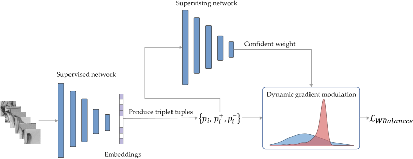
Figure 1: The calculation process of the proposed new loss function $\mathcal{L}_{WBalance}$.

Debiased Negative Sampling. In general, when the number of positive samples and candidate negative samples is not in the same order of magnitude, the same or even better results can be achieved by using a certain strategy to sample the negative ones for selection. In other research areas, except for normal HNS, it has been shown that showing semi-hard [35] or distance-weighted samples [36] when training the model will help the improvement of performance. In descriptor learning, previous static negative sampling methods [37, 38] did not change with training and cannot dynamically adapt and adjust the distribution of candidate negative samples, which makes it difficult to mine more favorable negative samples. With the proposed dynamic sampling strategy, in the field of descriptor learning, Balntas et al. [30] used triple edge loss and triple distance loss for random sampling of triplet tuples. Simo-Serra et al. [39] utilized a relatively shallow architecture based on pairwise similarity to exploit hard-negative mining.

The sampling strategy of HardNet [16] outperforms classical hard-negative mining and random sampling for softmin, triplet margin, and contrastive losses. However, considering the risk of introducing false negative instances, it is important to design an effective discriminant criterion to help identify negative samples with high quality that can really improve the model performance. In our paper, this criterion is designed and incorporated into curriculum learning using a self-supervised-like approach.

3 Methodology

3.1 Method Framework

Our novelties can be shown from two aspects - loss function and training strategy. The calculation process of our new loss function is shown in Fig. 1. For better representation, we refer to the network being trained as the supervised network and the network that provides information to guide the supervised network in training as the supervising network. The supervising network can be a descriptor network that has completed its training or can be acted by the supervised network that is currently being trained. The training patches are first input into the supervised network to generate the corresponding embeddings, then based on the distances calculated from embeddings we can select triplet tuples of batch size. The supervising network then recalculates the positive and negative distances of these triplet tuples and generates a confidence level for balancing the attention weight to guide the training of the supervised network. Finally, the weight produced by the supervising network will be integrated into the balance loss of the supervised network to form weighted balance loss for parameters update.

For the training strategy, we divide it into two stages: preliminary training and then annealing training. The main difference between them is that annealing training uses training data of decreasing difficulty, which can further improve the performance of the supervised network.

3.2 Loss Function

Compared with triplet loss, our new loss function removes the positive margin (t in Eq. 9 from the loss function, and the strategy of gradient modulation is changed to a strategy which is similar to constructing two potential wells for positive and negative distances. In the process of optimizing the parameters of the supervised network along the gradient descent direction, it is like the process that the two potential wells of positive and negative distances are constantly and dynamically adjusted and finally reach relative equilibrium, as shown in Fig. 2.

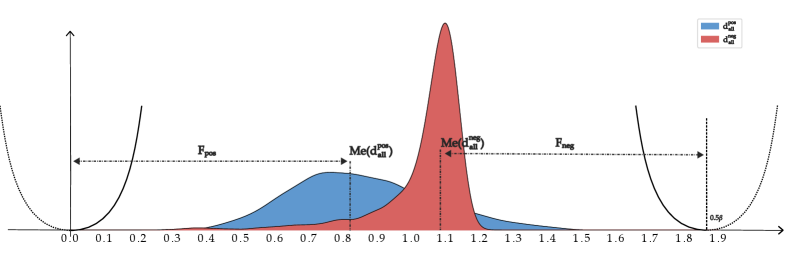
Figure 2: Schematic of the improved $\mathcal{L}_{Balance}$ and the superimposed distance distributions of $d_{neg}$ and $d_{pos}$. The $y$-axis represents the value of the loss function or the distribution of $d_{neg}$ and $d_{pos}$ in a batch. The $x$-axis represents the $L_{2}$ distance between the samples in a pair. The two curves represent the similarity measure functions ($S^{pos}$ and $S^{neg}$). The loss function is optimized to become smaller, which behaves like falling into two potential wells ( potential wells is a region in space where the potential energy of a particle is lower than its surrounding environment) and eventually reaching equilibrium.

Note that, in this paper we only use $L_{2}$ distance for descriptors similarity measure, so the negative distance and positive distance in a single triplet can be represented as:

where we have used the terms positive, negative, and anchor for corresponding ${x}_{i}^{+}$, ${x}_{i}^{+}$, ${x}_{i}$ in a triplet tuple in the following sections. Note that ${x}_{i}^{+}$ can represent more than one term if there are multiple positives, depending on how many positives are available in the dataset. When there are several positives available for an anchor in the used dataset, we will choose the positive with the largest distance from the anchor ${x}_{i}$. This is similar to a hard positive mining strategy, and we note that it can slightly improve performance.

3.2.1 Determination of similarity measure function

At this stage, our overall loss function can be expressed as:

$$\mathcal{L}_{Balance}=\frac{1}{N}\sum_{i=1}^{N}\left(s_{i}^{neg}+s_{i}^{neg}\right).$$ (2)

And the similarity measure function $s(d)$ can be defined as two exponential functions:

$$\begin{array}[]{c}s_{i}^{pos}=\left(d_{i}^{pos}-P_{pos}\right)^{\alpha},\\ \\ s_{i}^{neg}=\left(d_{i}^{neg}-P_{neg}\right)^{\alpha}.\\ \end{array}$$ (3)

The key required to characterize the similarity measure function is to determine the zero position, where is the position of the derivative of $s(d)$ intersects the x-axis (0.5$\beta$ in Fig. 4) and represented as $P_{neg}$ and $P_{pos}$. As the samples of each batch change with different HNS and different model learning stages, they should be dynamically adjusted by the information from the sample distribution in a batch to make the settings of the similarity measure function at different stages more appropriate for the current model learning situation. The visualization of data distribution as training proceeds is shown in Fig. 3.

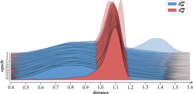
Figure 3: Positive and negative distance distributions with different epochs. As the training progresses the positive distance distribution tends to move in the positive direction of the x-axis, while the negative distance distribution tends to move in the opposite direction.

According to the distribution information in a batch, We define zero positions of the similarity measure functions dynamically:

$$\begin{array}[]{c}P_{pos}=Me\left(d_{all}^{neg}\right)-F_{pos},\\ \\ P_{neg}=Me\left(d_{all}^{neg}\right)+F_{neg},\end{array}$$ (4)

where $Me$ is a method to get the median in a batch of positive or negative distances, $P_{neg}$ and $P_{pos}$ are zero positions of the corresponding similarity measure functions of negative and positive part. $F_{pos}$ and $F_{neg}$ are focusing intensities which are used to adjust how much attention is paid to the hard samples and can be represented as distance between $P_{pos}$ and $Me\left(d_{all}^{neg}\right)$ shown in Fig. 2. Based on the assumption that there is a strong correlation between these two distances which are calculated by the zero positions and the corresponding center of the distribution, we can link the two focusing intensities with:

$$\begin{array}[]{c}\gamma F_{pos}=F_{neg},\end{array}$$ (5)

where $\gamma$ is a hyperparameter to adjust the ratio between the two focusing intensities.

For positive distribution, ${d_{i}^{neg}}$ is a positive value representing the distance between positive and anchor which should be minimized by the model. So we set $P_{pos}$ always situated at zero and only regulating $P_{neg}$ for simplification. Combining Eq. 4 and Eq. 5, we get the formula to calculate $P_{neg}$:

$$\begin{array}[]{c}P_{neg}={\gamma}Me\left(d_{all}^{neg}\right)+Me\left(d_{all}^{neg}\right),\\ \end{array}$$ (6)

where its value varies with the training process. This dynamic regulation reduces the trouble of over-parameterization and contributes to the stability of the final performance.

3.2.2 Adaptive weight assignment of gradient

To make $\mathcal{L}_{Balance}$ serve to minimize the positive distance and maximize the negative distance, we define different similarity measure functions $s(d)$ for positive and negative distances to determine the direction and magnitude of the gradient descent, which can achieve adaptive weight assignment of gradient. The following is the proof.

Combined with Eq. 3 and Eq. 1, the derivative of our overall loss can be represented as:

$N$ denotes the batch size, $D$ denotes $\left\{p_{1},p_{2},\ldots,p_{N};p_{1}^{+},p_{2}^{+},\ldots,p_{N}^{+}\right\}$ representing all embeddings of the corresponding patches in a batch. $p_{i}^{-}$ and $p_{i}^{+}$ represent the selected patch embeddings that have the maximum or minimum distance from the anchors. In our settings, $\frac{\partial\mathcal{L}}{\partial S_{i}^{pos}}$ is equal to 1 for positive and negative similarity measure functions, so the above equation can be reduced to

Note that in Eq. 8, $\alpha$ is selected to range from even numbers greater than or equal to 2 and $\alpha\left(d_{i}^{neg}-P_{neg}\right)^{\alpha-1}$ is a negative number when it comes to actual training, so the direction of gradient decline is consistent with the triplet loss. The original triplet loss and its derivative can be represented as:

$$\mathcal{L}_{Triplet}=\frac{1}{N}\sum_{i=1}^{N}\max\left(0,t+d_{i}^{neg}-d_{i}^{neg}\right),$$ (9)

when compared Eq. 7 with Eq. 10, $\frac{\partial S_{i}^{pos}}{\partial d_{i}^{pos}}$ and $\frac{\partial S_{i}^{neg}}{\partial d_{i}^{neg}}$ are the terms that differentiate the derivative of balance loss and the derivative of triplet loss. In $s(d)$ the introduction of the exponential term allows the updated weight of gradient to automatically fit the size of the distance between samples. The behaviors of triplet loss and balance loss and their derivatives are shown and compared in Fig. 4.

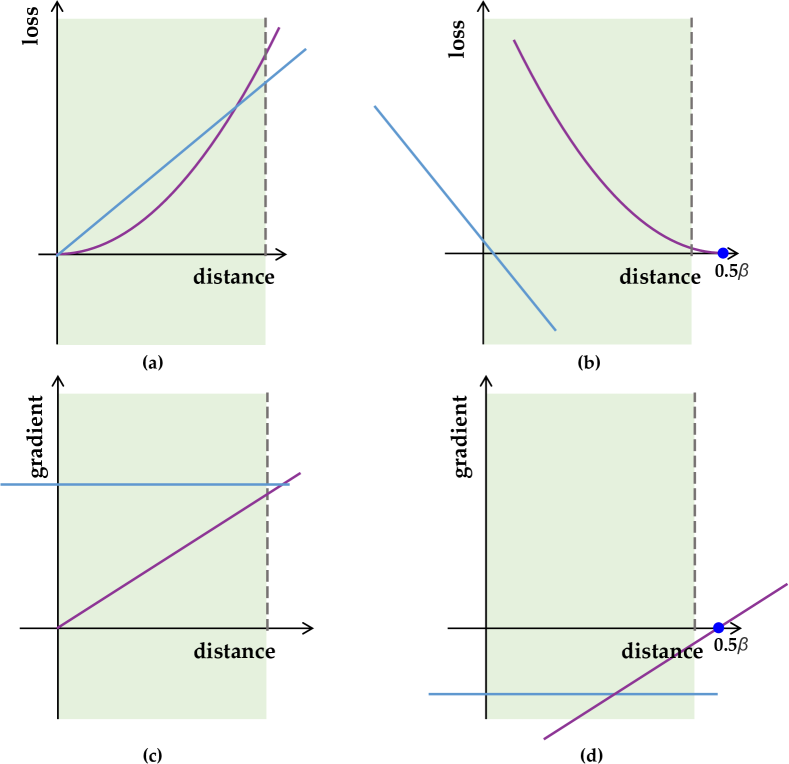
Figure 4: Comparison of two different loss functions and their derivatives. Purple indicates our improvement, blue indicates triplet loss. The green region is the actual distribution range of $L_{2}$ distance after normalization, which indicates the action range of loss functions.

In the backpropagation of balance loss, due to the similarity measure functions $s(d)$, the derivation of the network will generate additional functions with respect to the value of distances. Usually, we can set them as a primary function so that their values vary linearly with the increase or decrease of distances, as shown in Fig. 4 (c, d), so that the network can pay more attention and produce larger weight for embeddings with smaller ${d_{i}^{neg}}$ and larger ${d_{i}^{pos}}$ in the backpropagation process of each batch.

3.2.3 Negative sampling unbiased processing

The adaptive weighting in the loss function is designed to modulate the gradient based on information about the distribution of individual pairs with positive or negative distances, which makes the network more focused on the hard negative samples. In this case, the negative sampling unbiased processing measures the relative distance in triplet pairs to mitigate the negative impact of potentially false negative samples or overly difficult negative samples so that the attention on these samples is reduced. Specifically, we propose to use a supervising network to help the model identify these outliers and reduce their weight.

We can use either the training model (i.e., the supervising network and the supervised network are the same networks) or a pre-trained model, which is similar to knowledge distillation [40], as the supervising network. The difference is that the output of this supervising model is not labels, but the confidence level of the original labels for some samples. First, we define $I$ to represent the confidence level of the labels for positive and negative samples, which are dynamically selected during training:

$${I_{i}=d_{i}^{pos}-d_{i}^{neg}.}$$ (11)

Note that ${d_{i}^{neg}}$ and ${d_{i}^{neg}}$ are calculated by the embedding output of the supervising network for the triplet tuples which are selected by the supervised network through HNS. When ${d_{i}^{neg}}$ - ${d_{i}^{neg}}$$<upper$, this means the anchor is predicted to be more similar to the negative than the positive ones in a triplet tuple. When the supervising network makes this judgment, we need to determine the magnitude of the weight to be mitigated for that triplet tuple based on the value of $I$. So, we define $W_{i}$ can be calculated as:

$$W_{i}=\left\{\begin{array}[]{cc}f(I_{i}),&I_{i}\in[{upper,threshold}],\\ 1,&I_{i}>{upper},\\ 0,&I_{i}<{threshold},\end{array}\right.$$ (12)

where $W_{i}$ ranging form [0, 1] is the confident weight for each triplet tuple in a batch, and $f(\cdot)$ is the monotonic function that maps $I$ to the interval [0,1], which can usually be selected as an exponential function. $upper$ and $threshold$ are hyperparameters to determine the domain of the mapping function, as shown in Fig. 5.

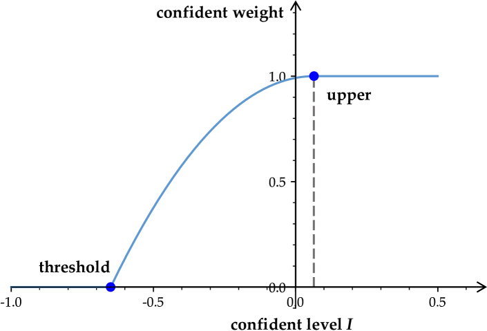
Figure 5: The blue curve represents the values of the confident weight calculated by the $W_{c}$ function with different $I$ values.

Finally, our weighted balance loss can be expressed as:

$$\mathcal{L}_{WBalance}=\frac{1}{N}\sum_{i=1}^{N}\ W_{i}\left(s_{i}^{neg}+s_{i}^{neg}\right).$$ (13)

Because the supervising network only needs to process the patches selected by the supervised network and calculate the distance each time, this approach does not incur excessive computational overhead and only increases the training time by about 10% when using the training model as the supervising network.

3.3 Annealing training

In the preliminary training, we used the strategy of hard negative mining and hard positive mining to select triplet tuples for gradient update. However, in the actual deployment and testing scenarios, the model needs to face a larger proportion of easy and medium difficult samples, so it is necessary to change the training strategy after the preliminary training is completed, i.e., to move from the strategy of selecting only the hardest samples to the strategy of selecting less difficult samples to improve the data generalization ability of the model in the actual testing scenarios.

Specifically, in annealing training, the weight of these triplets will be manually set to zero when $I_{i}<thr$ ($I_{i}$ calculated from Eq. 11), which means that they will not participate in the parameter update of the model. This process is iterative as shown in Algorithm 1. It means $bs$ and $thr$, represent the batch size and cut-off threshold, will be updated after each iteration according to:

$$\begin{array}[]{cc}bs_{t}=bs_{t-1}-stepsize_{bs},\\ thr_{t}=thr_{t-1}+stepsize_{thr},\end{array}$$ (14)

until the set final value is reached. And the initial learning rate $lr$ in one iteration is calculated by:

$$\begin{array}[]{cc}lr_{t}=lr_{t-1}*\epsilon^{t},\end{array}$$ (15)

where $\epsilon$ is the learning rate decay factor.

Algorithm 1 Annealing training algorithm

1:  Initialization: current batch size $bs$, iteration started batch size $bs_{s}$, iteration ended batch size $bs_{e}$, current iteration threshold $thr$, step size for each threshold increase $stepsize_{thr}$, step size for each batch size decrease $stepsize_{bs}$, initial learning rate $lr$

2:  $n=(bs_{e}-bs_{s})/stepsize_{bs}$

3:  $t=0$

4:  while $t<n$ do

5:     Update $bs_{t},thr_{t}$ based on Eq. 14

6:     Update $lr_{t}$ based on Eq. 15.

7:     Update the hyperparameters in annealing training of the current model as $bs_{t},lr_{t},thr_{t}$.

8:     Start training in this iteration:

9:     for a triplet $i$ in a batch do

10:        if  $I_{i}<thr_{t}$ for triplet $i$ then

11:           The weight of triplet $i$ will be set to zero, which means it will not participate in the process of model parameter update

12:        else

13:           Triplet $i$ will participate normally in the process of model parameter update

14:        end if

15:     end for

16:     Construct overall loss by Eq. 13 in a batch

17:     Backpropagation and model update

18:     End training in this iteration

19:     $t=t+1$

20:  end while

20:  Well-trained model after annealing training

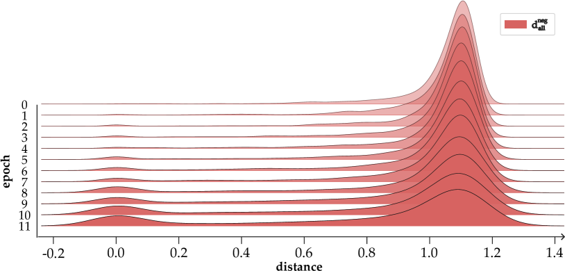
Figure 6: Density distribution of $W_{c}*{d_{all}^{neg}}$ with different epochs in annealing training. The visualization is performed by taking the first batch in each iteration.

The example of actual distribution of $W_{c}*{d_{all}^{neg}}$ is shown in Fig. 6. As annealing training proceeds, the samples used for training will gradually have a larger value of confidence level $I$, because the weight of triplets with low $I$ is set to 0 in $W_{c}$. This is shown in the figure - the number of negative distances located at the zero position of the $x$-axis becomes larger.

The key to annealing is that the batch size gradually decreases after each iteration, while the threshold gradually increases. We define the value of $I$ calculated from Eq. 11 for a triplet tuple as the basis for judging the difficulty of a sample. In this case, the increasing ${thr}$ will force the samples with decreasing difficulty in each batch to be used for updating the model after each iteration. Decreasing the batch size means that the probability of extracting a hard negative becomes smaller and the proportion of easy samples increases after each iteration.

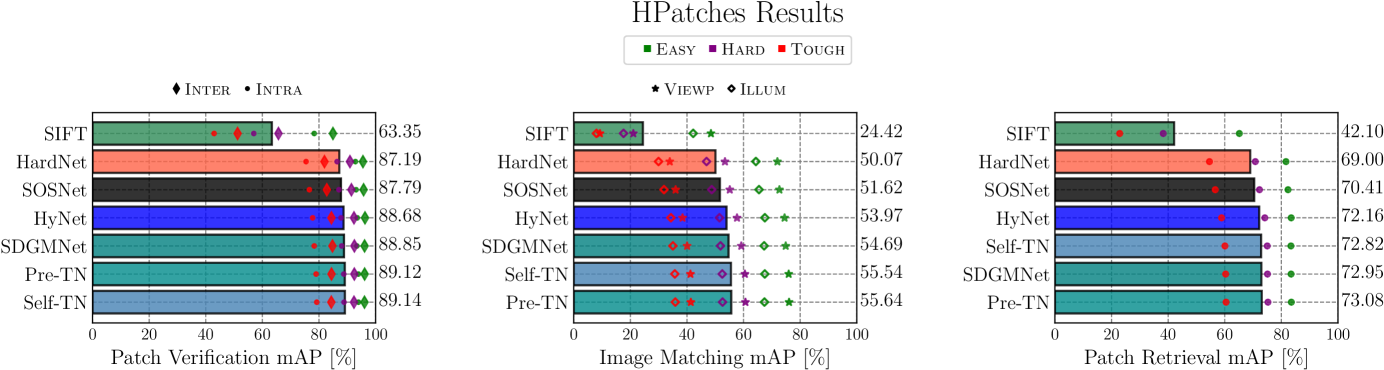
Figure 7: We tested the data split ’a’ of the HPatches benchmark following the standard protocol. All networks were trained on the Liberty dataset from UBC PhotoTour. The bar chart shows the average scores of the networks for the three subtasks Patch Verification, Image Matching, and Patch Retrieval, evaluated as mean average precision (mAP).

4 Experiment and result

4.1 Training Strategy

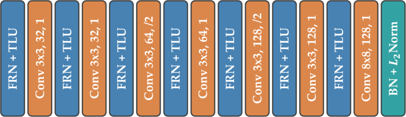
Figure 8: The network architecture is the same as that proposed by HyNet [12] with a dropout rate of 0.3.

Preliminary training. We used PyTorch to implement XXNet. As shown in Fig. 8, for a fair comparison, the network architecture is the same as that proposed by HyNet [12] and has the same amount of parameters as HardNet [16]. In the specific implementation of balance loss, we set $\alpha$=2, $\gamma$=1.05, and in the process of outliers we set supervising network with $upper$=0.065 and $threshold$=-0.65. The optimal model was trained with 25 epochs with 4050000 tuples per epoch and batch size=2560. Adam optimizer was used to update parameters with max lr=0.033, specifically using linear warm-up and cosine decay strategy for learning rate.

In Eq. 3, $\alpha$ is a scalar. Normally, $\alpha$ can be set equal to larger than 1 to represent an exponential function. We found a number larger than 2 does not necessarily lead to better results, so in the following experiments, we always set $\alpha$ equal to 2.

Annealing training. In AT, we tried to use triplet tuples of decreasing difficulty to update the network parameters at small learning rates. Specifically, the decrease in difficulty was achieved by setting the batch size to decrease by $stepsize_{bs}$=128 per iteration and the threshold to increase by $stepsize_{thr}$=0.05. Other parameters included: $bs_{s}$=2944, $bs_{e}$=1024, initial $thr$=-0.05, number of batches per iteration=1400. We also set the initial $lr$=$1.5*10^{-6}$ with a decay factor $\epsilon$=0.75 for each iteration.

4.2 Experiment Settings

We compared the performance of our solution with the state of the art on three benchmarks: UBC benchmark [28], HPatches [24] and IMC2020 [9]. We implemented two versions of the scheme, one using the training model as the supervising network called Self-TN and the other using a pre-trained supervising network with more parameters called Pre-TN.

UBC Benchmark evaluated on the Brown dataset [28]. It is a widely used patch dataset for evaluating the performance of local descriptors. The dataset consists of three subsets for three different scenarios: Liberty, Yosemite, and Notredame. Typically, deep descriptor networks are trained on one subset and tested on the other two subsets. According to the standard protocol [28], the test verifies that the network can correctly determine the 100K matching and non-matching pairs in the two test subsets. The protocol evaluates the metric using the false-positive rate at 95% recall (FPR@95), and we reported the experimental results for our two versions, including the average over all subsets, in Table I.

TABLE I:   PATCH VERIFICATION PERFORMANCE ON UBC PHOTOTOUR. NUMBERS SHOWN ARE FPR@95 ($\%$) THAT ARE LOWER FOR BETTER. THE BEST SCORES ARE HIGHLIGHTED IN BOLD. DASH LINES INDICATE CHANGES OF MODELS. LIB: Liberty, YOS: Yosemite, ND: Notredame.

Train	ND	YOS		LIB	YOS		LIB	ND	Mean
Test	LIB			ND			YOS
SIFT [25]	29.84			22.53			22.79		26.55
TFeat [30]	7.39	10.13		3.06	3.80		8.06	7.24	6.64
L2Net [14]	2.36	4.70		0.72	1.29		2.57	1.17	2.23
HardNet [16]	1.49	2.51		0.53	0.78		1.96	1.84	1.51
CDFDesc [18]	1.21	2.01		0.39	0.68		1.51	1.29	1.38
SOSNet [11]	1.08	2.12		0.34	0.67		1.03	0.95	1.03
HyNet [12]	0.89	1.37		0.34	0.61		0.88	0.96	0.84
Ours	0.86	1.32		0.30	0.57		0.80	0.91	0.79

HPatches [24] is a more comprehensive benchmark that evaluates descriptors on three tasks: patch verification, image matching and patch retrieval. According to geometric distortion, subtasks are categorized into Easy, Hard and Tough. Furthermore, patch pairs from the same or different image sequences are separated into two test subsets for verification, denoted by Intra and Inter, respectively. And the matching task is designed to evaluate the viewpoint (VIEWP) and illumination (ILLUM) invariance of descriptors.

Image Matching Challenge (IMC). IMC2020 is a large-scale challenge dataset of wide baseline matching [9]. IMC2020 consists of datasets with large illumination and viewpoint variations. In this experiment, we compare our method with the existing descriptors in an two-stage image matching pipeline. We experiment on the stereo track using the validation sets of Phototourism. This benchmark takes the predicted matches as input and measures the 6 DoF pose estimation accuracy. We measure the mean average accuracy (mAA) of pose estimation at $10^{\circ}$ and the number of inliers.

5 Discussion

In this section, we discuss the contribution of each component of XXNet to the overall performance and its influencing factors. Specifically, we trained different models on Liberty [28] and tested them on the Hpatches [24] matching task to obtain the influence of our three modifications - loss function, negative sampling unbiased processing, and annealing training - on the performance of the model.

Furthermore, we observed that a better FRP@95 metric does not necessarily imply a better mAP metric, which we believe is due to the fact that the FRP@95 metric is more concerned with the model’s ability to identify difficult samples and does not reflect how well the model fits all samples. This is related to the way FRP@95 is calculated. To better assess the performance of the model on all samples, we use mAP as the metric for the following test.

5.1 Ablation Study

TABLE II: Ablation experiments to explore the performance gains of each modification. The result is tested on data split ’full’ from the HPatches benchmark. mAP score for subtask image matching is reported.

Modification	Choice	Add unbiased processing	MAP(%)
	Triplet loss	$\usym{2717}$	55.67
Loss function	Triplet loss	$\checkmark$	56.08
	Balance loss	$\usym{2717}$	56.53
	Balance loss	$\checkmark$	56.83
Annealing training	AT+Triplet loss	$\usym{2717}$	56.25
	AT+Triplet loss	$\checkmark$	56.59
	AT+Balance loss	$\usym{2717}$	57.01
	AT+Balance loss	$\checkmark$	57.35

Loss function. The performance improvement of balance loss compared with triplet loss is shown in LABEL:{tabl:Abl}, and it is more significant after adding unbiased processing. Also, unbiased processing can be applied to the original triplet loss to improve performance. The influence of the magnitude of $\gamma$ value on the final mAP performance of the model can be seen in the Fig. 9(a). According to the previous Eq. 6, the $\gamma$ can be interpreted as a parameter here that balances the update weight between positive and negative distances. Specifically, a value greater than 1 leads to a greater update weight for negative part, and a value less than 1 indicates a greater update weight for positive part. Through hyperparameter search, we found that the model achieved the highest mAP performance when A=1.05 for the current training settings. Fig. 9(d) shows how the position of $P_{neg}$ changes as training progresses during the preliminary training process, and it can be observed a tendency for the value of $P_{neg}$ to become progressively smaller, implying the adjustment of our dynamic loss function.

In the sampling unbiased processing, the hyperparameter values of $upper$ and $threshold$ can be used to adjust the mitigation of weight for hard samples. Usually, the higher the threshold value means the higher the magnitude of alleviation, and the higher the upper value means the higher the number of samples involved in mitigation. The influence of $upper$ and $threshold$ on performance is shown in Fig. 9(b). In addition, for models that can achieve similar performance in preliminary training, we found that selecting models that trained at a lower $threshold$ and a lower $upper$ conditions as possible could lead to larger performance improvement in subsequent annealing training.

(a)

(b)

(c)

(d)

Figure 9: Experiments on the effect of hyperparameters on performance after preliminary training. The four figures are (a): The effect of hyperparameter $\gamma$ on the model performance. (b): The effect of hyperparameters $threshold$ and $upper$ on the model performance. (c): The effect of adding the supervising network (TNet) on the balance loss. (d): Adaptive changes of $P_{neg}$ values during gradient modulation.

Supervising network. Original HNS tends to extract samples that are difficult to be identified by the current model as the number of training epochs increases. As the difficulty of the samples increases, the proportion of triplet tuples that are worth learning in the samples gradually becomes smaller, resulting in a better fit of the model to extremely difficult samples and a decrease in performance in real-world-like test scenarios. Fig. 9(c) shows that as the number of training epochs increases, the mAP performance of the model on Hpatches full split tends to increase and then decrease. Compared with the previous one, the introduction of the supervising network alleviates this problem in training and provides a more relaxed selection interval for the optimal model, without worrying about the timing of early stopping. At the same time, Fig. 9(c) shows the mean and variance of the performance using the balance loss (no unbiased processing) with 4 different random seeds trained after 22 epochs under the same settings, which has a larger variance compared with the balance loss. Thus, the supervising network can also help the supervised network to improve performance stability.

In addition, the selection of the hyperparameters is related to the performance and training settings of the supervising network used. In addition to using the supervised network itself as the supervising network (Self-TNet), we also choose a larger network trained on the Liberty dataset, which has twice the number of channels per layer compared to the student net and therefore outputs a 256-dimensional vector. The experimental result is shown as Pre-TNet. In terms of specific training settings, we observed that using the pre-trained network as the supervising network, which does not have the best performance, can guide the supervised network to achieve the highest mAP. Presumably, it is related to the difference in fitting ability caused by the difference in the number of parameters between the supervising network and the supervised network [41]. Finally, we choose the network trained by balance loss with a fixed $\beta$ value and mining negative number equals 2 as the supervising network to guide the supervised network. Although the trained supervising network cannot achieve the optimal performance, it is beneficial for the supervised network to receive more information about the overall data distribution from the supervising network in the guidance.

Annealing training. The main hyperparameters in AT are the step sizes of $bs$ and $thr$. In this paper, we use $bs$ decreasing by 128 at a time and $thr$ increasing by 0.05 at a time as a general adjustment strategy. In general, smaller step sizes mean smoother transitions between the two training phases and usually better performance, but they also increase the computational cost. Here we balance the effects of both to choose the hyperparameters.

Figure 10: The performance of the original loss function before and after annealing training and the performance of balance loss before and after annealing training were compared

AT has a similar effect on the performance improvements shown in Fig. 10, as long as the model has previously undergone the HNS process. In addition, we can see from Fig. 10 that the model trained with balance loss can get more performance improvement in the annealing training. This can be attributed to the fact that the balance loss can handle the difficulty of the training samples by assigning more appropriate adaptive weights than the triplet loss, thus helping to learn more abstract laws from the samples. This proves that our two improvements can collaborate to provide the best performance.

6 Conclusion

In this paper, we investigated how to obtain and utilize high quality negative samples in the widely used hard negative sampling strategy in metric learning, trying to balance the difficulty of the HNS extraction samples to provide the learning samples which are most suitable for the training of the current model. The proposed balance loss combines the self-supervised method into a specific dynamic gradient modulation strategy to achieve fine-grained gradient modulation for different difficulty samples. The proposed annealing training provides data sources with different difficulty distributions for the loss function, which can alleviate the overfitting of hard samples in the training process and help the model to learn the general laws from the data. Our improved local descriptors show superiority on a variety of tasks and datasets.

References

- [1] J. Ma, J. Zhao, J. Tian, A. L. Yuille, and Z. Tu, “Robust point matching via vector field consensus,” IEEE Transactions on Image Processing, vol. 23, no. 4, pp. 1706–1721, 2014.
- [2] J. L. Schonberger, F. Radenovic, O. Chum, and J.-M. Frahm, “From single image query to detailed 3d reconstruction,” in Proceedings of the IEEE Conference on Computer Vision and Pattern Recognition, 2015, pp. 5126–5134.
- [3] K. M. Yi, E. Trulls, V. Lepetit, and P. Fua, “Lift: Learned invariant feature transform,” in European conference on computer vision. Springer, 2016, pp. 467–483.
- [4] D. DeTone, T. Malisiewicz, and A. Rabinovich, “Superpoint: Self-supervised interest point detection and description,” in Proceedings of the IEEE conference on computer vision and pattern recognition workshops, 2018, pp. 224–236.
- [5] J. Revaud, P. Weinzaepfel, C. De Souza, N. Pion, G. Csurka, Y. Cabon, and M. Humenberger, “R2d2: repeatable and reliable detector and descriptor,” arXiv preprint arXiv:1906.06195, 2019.
- [6] M. Dusmanu, I. Rocco, T. Pajdla, M. Pollefeys, J. Sivic, A. Torii, and T. Sattler, “D2-net: A trainable cnn for joint description and detection of local features,” in Proceedings of the ieee/cvf conference on computer vision and pattern recognition, 2019, pp. 8092–8101.
- [7] K. Li, L. Wang, L. Liu, Q. Ran, K. Xu, and Y. Guo, “Decoupling makes weakly supervised local feature better,” in Proceedings of the IEEE/CVF Conference on Computer Vision and Pattern Recognition, 2022, pp. 15 838–15 848.
- [8] M. Tyszkiewicz, P. Fua, and E. Trulls, “Disk: Learning local features with policy gradient,” Advances in Neural Information Processing Systems, vol. 33, pp. 14 254–14 265, 2020.
- [9] Y. Jin, D. Mishkin, A. Mishchuk, J. Matas, P. Fua, K. M. Yi, and E. Trulls, “Image matching across wide baselines: From paper to practice,” International Journal of Computer Vision, vol. 129, no. 2, pp. 517–547, 2021.
- [10] J. Ma, X. Jiang, A. Fan, J. Jiang, and J. Yan, “Image matching from handcrafted to deep features: A survey,” International Journal of Computer Vision, vol. 129, no. 1, pp. 23–79, 2021.
- [11] Y. Tian, X. Yu, B. Fan, F. Wu, H. Heijnen, and V. Balntas, “Sosnet: Second order similarity regularization for local descriptor learning,” in Proceedings of the IEEE/CVF Conference on Computer Vision and Pattern Recognition, 2019, pp. 11 016–11 025.
- [12] Y. Tian, A. Barroso Laguna, T. Ng, V. Balntas, and K. Mikolajczyk, “Hynet: Learning local descriptor with hybrid similarity measure and triplet loss,” Advances in Neural Information Processing Systems, vol. 33, pp. 7401–7412, 2020.
- [13] K. He, Y. Lu, and S. Sclaroff, “Local descriptors optimized for average precision,” in Proceedings of the IEEE conference on computer vision and pattern recognition, 2018, pp. 596–605.
- [14] Y. Tian, B. Fan, and F. Wu, “L2-net: Deep learning of discriminative patch descriptor in euclidean space,” in Proceedings of the IEEE conference on computer vision and pattern recognition, 2017, pp. 661–669.
- [15] V. Kumar BG, G. Carneiro, and I. Reid, “Learning local image descriptors with deep siamese and triplet convolutional networks by minimising global loss functions,” in Proceedings of the IEEE conference on computer vision and pattern recognition, 2016, pp. 5385–5394.
- [16] A. Mishchuk, D. Mishkin, F. Radenovic, and J. Matas, “Working hard to know your neighbor’s margins: Local descriptor learning loss,” Advances in neural information processing systems, vol. 30, 2017.
- [17] X. Wei, Y. Zhang, Y. Gong, and N. Zheng, “Kernelized subspace pooling for deep local descriptors,” in Proceedings of the IEEE conference on computer vision and pattern recognition, 2018, pp. 1867–1875.
- [18] L. Zhang and S. Rusinkiewicz, “Learning local descriptors with a cdf-based dynamic soft margin,” in Proceedings of the IEEE/CVF International Conference on Computer Vision, 2019, pp. 2969–2978.
- [19] S. Wang, Y. Li, X. Liang, D. Quan, B. Yang, S. Wei, and L. Jiao, “Better and faster: Exponential loss for image patch matching,” in Proceedings of the IEEE/CVF International Conference on Computer Vision, 2019, pp. 4812–4821.
- [20] J. Wang, F. Zhou, S. Wen, X. Liu, and Y. Lin, “Deep metric learning with angular loss,” in Proceedings of the IEEE international conference on computer vision, 2017, pp. 2593–2601.
- [21] H. Wang, Y. Wang, Z. Zhou, X. Ji, D. Gong, J. Zhou, Z. Li, and W. Liu, “Cosface: Large margin cosine loss for deep face recognition,” in Proceedings of the IEEE conference on computer vision and pattern recognition, 2018, pp. 5265–5274.
- [22] X. Wang, X. Han, W. Huang, D. Dong, and M. R. Scott, “Multi-similarity loss with general pair weighting for deep metric learning,” in Proceedings of the IEEE/CVF Conference on Computer Vision and Pattern Recognition, 2019, pp. 5022–5030.
- [23] C.-Y. Chuang, J. Robinson, Y.-C. Lin, A. Torralba, and S. Jegelka, “Debiased contrastive learning,” Advances in neural information processing systems, vol. 33, pp. 8765–8775, 2020.
- [24] V. Balntas, K. Lenc, A. Vedaldi, and K. Mikolajczyk, “Hpatches: A benchmark and evaluation of handcrafted and learned local descriptors,” in Proceedings of the IEEE conference on computer vision and pattern recognition, 2017, pp. 5173–5182.
- [25] D. G. Lowe, “Distinctive image features from scale-invariant keypoints,” International journal of computer vision, vol. 60, no. 2, pp. 91–110, 2004.
- [26] H. Bay, T. Tuytelaars, and L. Van Gool, “Surf: Speeded up robust features,” in Computer Vision–ECCV 2006: 9th European Conference on Computer Vision, Graz, Austria, May 7-13, 2006. Proceedings, Part I 9. Springer, 2006, pp. 404–417.
- [27] Z. Wang, B. Fan, and F. Wu, “Local intensity order pattern for feature description,” in 2011 International Conference on Computer Vision. IEEE, 2011, pp. 603–610.
- [28] M. Brown, G. Hua, and S. Winder, “Discriminative learning of local image descriptors,” IEEE transactions on pattern analysis and machine intelligence, vol. 33, no. 1, pp. 43–57, 2010.
- [29] X. Han, T. Leung, Y. Jia, R. Sukthankar, and A. C. Berg, “Matchnet: Unifying feature and metric learning for patch-based matching,” in Proceedings of the IEEE conference on computer vision and pattern recognition, 2015, pp. 3279–3286.
- [30] V. Balntas, E. Riba, D. Ponsa, and K. Mikolajczyk, “Learning local feature descriptors with triplets and shallow convolutional neural networks.” in Bmvc, vol. 1, no. 2, 2016, p. 3.
- [31] Z. Luo, T. Shen, L. Zhou, J. Zhang, Y. Yao, S. Li, T. Fang, and L. Quan, “Contextdesc: Local descriptor augmentation with cross-modality context,” in Proceedings of the IEEE/CVF conference on computer vision and pattern recognition, 2019, pp. 2527–2536.
- [32] Z. Luo, T. Shen, L. Zhou, S. Zhu, R. Zhang, Y. Yao, T. Fang, and L. Quan, “Geodesc: Learning local descriptors by integrating geometry constraints,” in Proceedings of the European conference on computer vision (ECCV), 2018, pp. 168–183.
- [33] Y. Sun, C. Cheng, Y. Zhang, C. Zhang, L. Zheng, Z. Wang, and Y. Wei, “Circle loss: A unified perspective of pair similarity optimization,” in Proceedings of the IEEE/CVF Conference on Computer Vision and Pattern Recognition, 2020, pp. 6398–6407.
- [34] M. Keller, Z. Chen, F. Maffra, P. Schmuck, and M. Chli, “Learning deep descriptors with scale-aware triplet networks,” in Proceedings of the IEEE Conference on Computer Vision and Pattern Recognition, 2018, pp. 2762–2770.
- [35] F. Schroff, D. Kalenichenko, and J. Philbin, “Facenet: A unified embedding for face recognition and clustering,” in Proceedings of the IEEE conference on computer vision and pattern recognition, 2015, pp. 815–823.
- [36] C.-Y. Wu, R. Manmatha, A. J. Smola, and P. Krahenbuhl, “Sampling matters in deep embedding learning,” in Proceedings of the IEEE international conference on computer vision, 2017, pp. 2840–2848.
- [37] E. Diaz-Aviles, L. Drumond, L. Schmidt-Thieme, and W. Nejdl, “Real-time top-n recommendation in social streams,” in Proceedings of the sixth ACM conference on Recommender systems, 2012, pp. 59–66.
- [38] S. Rendle, C. Freudenthaler, Z. Gantner, and L. Schmidt-Thieme, “Bpr: Bayesian personalized ranking from implicit feedback,” arXiv preprint arXiv:1205.2618, 2012.
- [39] E. Simo-Serra, E. Trulls, L. Ferraz, I. Kokkinos, P. Fua, and F. Moreno-Noguer, “Discriminative learning of deep convolutional feature point descriptors,” in Proceedings of the IEEE international conference on computer vision, 2015, pp. 118–126.
- [40] G. Hinton, O. Vinyals, J. Dean et al., “Distilling the knowledge in a neural network,” arXiv preprint arXiv:1503.02531, vol. 2, no. 7, 2015.
- [41] J. Gou, B. Yu, S. J. Maybank, and D. Tao, “Knowledge distillation: A survey,” International Journal of Computer Vision, vol. 129, pp. 1789–1819, 2021.