Decomposition of zero-dimensional persistence modules via rooted subsets

Abstract.

We study the decomposition of zero-dimensional persistence modules, viewed as functors valued in the category of vector spaces factorizing through sets. Instead of working directly at the level of vector spaces, we take a step back and first study the decomposition problem at the level of sets.

This approach allows us to define the combinatorial notion of rooted subsets. In the case of a filtered metric space $M$, rooted subsets relate the clustering behavior of the points of $M$ with the decomposition of the associated persistence module. In particular, we can identify intervals in such a decomposition quickly. In addition, rooted subsets can be understood as a generalization of the elder rule, and are also related to the notion of constant conqueror of Cai, Kim, Mémoli and Wang. As an application, we give a lower bound on the number of intervals that we can expect in the decomposition of zero-dimensional persistence modules of a density-Rips filtration in Euclidean space: in the limit, and under very general circumstances, we can expect that at least 25% of the indecomposable summands are interval modules.

1. Introduction

Multiparameter persistent homology is an active research area in topological data analysis. The motivation is that in many datasets there are multiple parameters that deserve attention in a multiscale analysis [18, 32, 11]. Concretely, when analyzing point clouds, we want to consider the distances between points, but also potentially remove points of low density.

A central object of persistent homology is the persistence module, which tracks algebraically how the topological features of the data change as we move through the parameter space. In the single-parameter case, every persistence module decomposes into a collection of intervals, called the persistence barcode [20], where each interval represents the lifetime of a topological feature in the data. In the multiparameter setting, there is a generalized notion of interval, which again represents the lifetime of a topological feature, but decomposing a multiparameter persistence module into intervals is not always possible, and one might be left with non-interval indecomposable persistence modules that lead to complications, both theoretically [18, 12, 13, 33] and computationally [23, 1, 4].

In fact, the classification of such indecomposable persistence modules is thought to be out of reach: certain involved posets are of wild representation type, even when accounting for certain simplifications [2]. Moreover, infinite families of complicated indecomposable persistence modules can be realized by simple geometric constructions [13], and, most recently, it has been shown in [3] that multiparameter persistence modules are, generically, close to being indecomposable, under the interleaving metric (we refer to [3] for a precise statement).

Still, the mentioned complications do not imply that the persistence modules that come up in practice are close to indecomposable, or that they are not decomposable into intervals. Indeed, is the decomposition of multiparameter persistence modules as badly behaved in practice as we can expect in theory? The authors of [2] and those of [3] state similar questions.

As an initial test, we computed the decomposition of persistence modules for a standard zero-dimensional construction, using a prototypical implementation of the algorithm by Dey and Xin [23] (this implementation will be discussed in another paper). As we see in Table 1, the assumption that persistence modules can be decomposed completely into intervals seems to be false most of the time, at least in this setting. However, Table 1 also shows that in all tested instances, most indecomposable summands are indeed intervals.

Table 1. Number of intervals in the decomposition of zero-dimensional persistence modules for density-Rips filtrations. We tried both clustered samples where the points were sampled by a multivariate Gaussian distribution around $5$ peaks, and uniform samples in the unit square. The density parameter was computed via a Gaussian kernel density estimate (kde) or a random density was assigned. The table shows the number of intervals for $5$ independent test runs; for $n$ points, the module is interval-decomposable if the number of intervals is $n$. This only happens for one run.

		100 points					500 points
Sample	Densities	Run 1	2	3	4	5	Run 1	2	3	4	5
clustered	kde	100	98	95	98	98	474	487	478	479	479
uniform	kde	88	88	86	88	86	444	447	433	453	457
clustered	random	77	86	87	88	76	397	381	390	380	386
uniform	random	76	79	75	75	70	376	361	366	355	377

This begs the question whether we can provably expect many intervals in general. In addition, knowledge of the intervals can greatly simplify and speed up computational tasks for persistence modules: for instance, a popular way to analyze 2-parameter persistence modules is by considering $1$-dimensional restrictions, so-called slices, resulting in a parameterized family of persistent barcodes [29, 34, 35, 32]. Every interval of the $2$-dimensional persistence module gives one bar in the barcode of the slice, by intersecting the slice with the interval. Thus, by knowing the intervals, existing algorithms can focus on the non-interval “core” of the problem, which is typically of much smaller size.

The practical problem of the described approach is that decomposing a multiparameter persistence module is costly, despite ongoing efforts [23]. However, to leverage the knowledge of intervals there is no need to compute a total decomposition, or to even identify all intervals. It suffices to have a method to “peel off” intervals from a persistence module quickly. Thus, we pose the question whether there exist methods that work very fast in practice and still are capable of detecting many intervals.

Contributions.

We focus on the case of zero-dimensional persistence modules. Already this case is of practical interest because of its connection to hierarchical clustering methods (see the Related work section below), and has received attention recently [14, 2, 35, 10]. In this context, we give some answers to the questions stated above:

For a point cloud $M$, a nearest neighbor pair is a pair $(x,y)\in M\times M$ such that $y$ is the nearest neighbor of $x$ and $x$ is the nearest neighbor of $y$ (breaking ties with a fixed total order). The theory we develop says that for a zero-dimensional persistence module of the density-Rips bifiltration (for any density estimation function), there are at least as many intervals as there are nearest neighbor pairs in $M$. These intervals are easily determined by the nearest neighbor pairs, and we refer to them as NN-intervals. Since all nearest neighbor pairs can be computed in $O(n\log n)$ time [19, 38], this yields a fast method to compute all NN-intervals of the decomposition. Moreover, we can expect many NN-intervals: using previous results on nearest neighbor graphs, we show that if $M$ is sampled independently from an arbitrary, almost continuous density function, at least a quarter of the summands in the decomposition are intervals as $n\to\infty$. To our knowledge, this is the first result proving a non-constant lower bound on the number of intervals in a decomposition.

To arrive at this result, we use the following main idea: Instead of studying the decomposition of the persistence module directly in the category of (graded) vector spaces, we work in the category of persistent sets, whose objects can be interpreted as a two-parameter hierarchical clustering. The decomposition of a persistence module is governed by its idempotent endomorphisms, so we look for idempotent endomorphisms not of persistence modules, but of persistent sets, which are simpler. We show that such idempotent endomorphisms can be translated into rooted subsets, which are subsets of points that get consistently merged with a fixed point in the hierarchical clustering. Moreover, rooted subsets with a single element correspond to intervals in the associated persistence module.

Instead of peeling off intervals from the persistence module, we peel off rooted subsets from the persistent set. The advantage is that the remaining structure is still a hierarchical clustering, and the process can be iterated.

Related work.

Multiparameter persistent sets and zero-dimensional persistence modules, as we will study them here, are related to a multiparametric approach to the clustering problem first considered by Carlsson and Mémoli [16]. The need for multiple parameters, density and scale, is justified by an axiomatic approach to clustering [28, 15, 17]. The application of techniques from multiparameter persistence homology, like persistence modules and interleavings, to this setting has attracted attention recently [32, 14, 2, 35, 34].

Cai, Kim, Mémoli, and Wang [14] define a useful summary for zero-dimensional persistence modules coming from density-Rips, called the elder-rule-staircode, inspired by the elder rule [24]. They also introduce the related concept of constant conqueror, and they ask whether a constant conqueror induces an interval in the decomposition of the associated persistence module. We answer this question in the negative with Example 4.3, and, in contrast, we show that a rooted generator, as introduced here, does induce an interval in the decomposition (Corollary 3.7).

Brodzki, Burfitt, and Pirashvili [10] also study the decomposition of zero-dimensional persistence modules. They identify a class of persistence modules, called semi-component modules, that may appear as summands in the decomposition of zero-dimensional modules, but that are still hard to classify. Their methods have been of great inspiration, and in Theorem 5.1 we give another proof, within the theory we develop, of a theorem of theirs.

Acknowledgements.

The authors thank Jan Jendrysiak for helpful discussions. We are also grateful to the anonymous reviewers for their careful reading of our manuscript and their detailed comments and suggestions. This research has been supported by the Austrian Science Fund (FWF) grant P 33765-N.

2. Preliminaries

Persistent sets and persistence modules.

In what follows, we let $P$ be a finite poset, which we will view as a category. A persistence module (over $P$) is a functor from $P$ to the category $\mathsf{Vec}$ of finite dimensional vector spaces, over a fixed field $K$. Such a functor $F\colon P\to\mathsf{Vec}$ associates to each grade $p\in P$ a finite dimensional vector space $F_{p}$ and to each morphism $p\leq q$ in $P$ a linear map $F_{p\to q}\colon F_{p}\to F_{q}$, in such a way that $F_{p\to p}=\mathrm{id}$ and composition is preserved. We see persistence modules as the objects of the functor category $\mathsf{Vec}^{P}$, where natural transformations are the morphisms. In this sense, a morphism $f\colon F\to G$ of persistence modules is a family of maps $\{f_{p}\colon F_{p}\to G_{p}\}_{p\in P}$ such that for every two $p\leq q$ the following diagram commutes

Similarly, a persistent set (over $P$) is a functor from $P$ to $\mathsf{Set}$, the category $\mathsf{Set}$ of finite sets, and morphisms of persistent sets are natural transformations as above.

We can obtain a persistence module from a persistent set by the application of the linearization functor $\mathsf{Set}\to\mathsf{Vec}$ that takes each set to the free vector space generated by it. This linearization functor induces a functor $\mathcal{L}\colon\mathsf{Set}^{P}\to\mathsf{Vec}^{P}$ by postcomposition.

From geometry to persistent sets.

Let $(M,d)$ be a finite metric space, and consider a function $f\colon M\to\mathbb{R}$. We can understand $f$ as an assignment of a density to each of the points of $M$; that is, a density estimation function [37]. We assume that $f$ assigns lower values to points of higher density. Following [14], we call the triple $(M,d,f)$ an augmented metric space. We construct a persistent set, the density-Rips persistent set of $(M,d,f)$, that tracks how the clustering of points of $M$ changes as we change the density and scale parameters, in a sense that we make precise shortly.

First, for a fixed scale parameter $\varepsilon\geq 0$, we define the geometric graph of $M$ at $\varepsilon$, denoted by $\mathcal{G}_{\varepsilon}(M)$, as the undirected graph on the vertex set $M$ and edges $(x,y)$ where $d(x,y)\leq\varepsilon$. The connected components of $\mathcal{G}_{\varepsilon}(M)$, as $\varepsilon$ goes from $0$ to $\infty$, form the clusters of the dendrogram obtained via the single-linkage clustering method.

To introduce the density, for each $\sigma\in\mathbb{R}$ we let $M_{\sigma}\coloneqq\{x\in M\nonscript\>|{}\allowbreak{}\nonscript\>\mathopen{}f(x)\leq\sigma\}\subseteq M$ be the metric subspace of points with (co)density below $\sigma$. For any two $\sigma\leq\sigma^{\prime}$, $M_{\sigma}\subseteq M_{\sigma^{\prime}}$ and by taking each $(\varepsilon,\sigma)$ to the graph $\mathcal{G}_{\varepsilon}(M_{\sigma})$, we obtain a functor $\mathcal{G}(M,f)\colon\mathbb{R}_{\geq 0}\times\mathbb{R}\to\mathsf{Graph}$, where the order in $\mathbb{R}_{\geq 0}\times\mathbb{R}$ is given by $(\varepsilon,\sigma)\leq(\varepsilon^{\prime},\sigma^{\prime})$ if and only if $\varepsilon\leq\varepsilon^{\prime}$ and $\sigma\leq\sigma^{\prime}$. We then consider the connected components functor $\pi_{0}\colon\mathsf{Graph}\to\mathsf{Set}$, that takes each graph to its set of connected components. In this way, we obtain a functor $\pi_{0}\circ\mathcal{G}(M,f)\colon\mathbb{R}_{\geq 0}\times\mathbb{R}\to\mathsf{Set}$.

Remark 2.1.

The linearized persistence module $\mathcal{L}(\pi_{0}\circ\mathcal{G}(M,f))\colon\mathbb{R}_{\geq 0}\times\mathbb{R}\to\mathsf{Vec}$ is isomorphic to the persistence module obtained by applying zero-dimensional homology at graph level, $H_{0}\circ\mathcal{G}(M,f)\colon\mathbb{R}_{\geq 0}\times\mathbb{R}\to\mathsf{Vec}$. In this sense, the construction we have described is the zero-dimensional level of the density-Rips filtration, which is standard in multiparameter persistent homology (see [18, 5] and also [14]).

We can understand the functor $\pi_{0}\circ\mathcal{G}(M,f)\colon\mathbb{R}_{\geq 0}\times\mathbb{R}\to\mathsf{Set}$ as a persistent set $S\colon P\to\mathsf{Set}$ indexed by a finite grid $P\subseteq\mathbb{R}_{\geq 0}\times\mathbb{R}$ in the following way. We consider the set of distances $D\coloneqq\{d(x,y)\nonscript\>|{}\allowbreak{}\nonscript\>\mathopen{}x,y\in M\}$ and densities $T\coloneqq\{f(x)\nonscript\>|{}\allowbreak{}\nonscript\>\mathopen{}x\in M\}$, and define a finite grid $P\coloneqq D\times T\subset\mathbb{R}_{\geq 0}\times\mathbb{R}$. Finally, we define the persistent set $S\colon P\to\mathsf{Set}$ by taking each $(\varepsilon,\sigma)\in P$ to $(\pi_{0}\circ\mathcal{G}(M,f))_{(\varepsilon,\sigma)}$, and similarly for the morphisms.

Definition 2.2.

Let $(M,d,f)$ be an augmented metric space. We define its density-Rips persistent set as the functor $S\colon P\to\mathsf{Set}$, constructed as above.

Decomposition of persistence modules.

We can study persistence modules via their decomposition. For two persistence modules $F$ and $G$ their direct sum $F\oplus G$ is the persistence module given by taking direct sums pointwise, $(F\oplus G)_{p}=F_{p}\oplus G_{p}$. A persistence module is indecomposable if $F\cong F_{1}\oplus F_{2}$ implies that either $F_{1}=0$ or $F_{2}=0$. Since persistence modules are actual modules (see, for instance, [8, Lemma 2.1]), by the Krull-Schmidt theorem, a decomposition of a persistence module $F=F_{1}\oplus F_{2}\oplus\dots F_{n}$ into indecomposable summands is unique up to permutation and isomorphism of the summands.

Let $I$ be a non-empty connected subposet of a poset $P$ such that for any two $i,j\in I$ and any $l\in P$, if $i\leq l\leq j$ then $l\in I$. The interval module supported on $I$, $\mathcal{I}(I)\colon P\to\mathsf{Vec}$, is the indecomposable (by, e.g. [7, Proposition 2.2]) persistence module given by

$$\mathcal{I}(I)_{p}=\begin{cases}K,&\text{if $p\in I$,}\\ 0,&\text{otherwise,}\end{cases}\quad\text{with internal maps}\quad\mathcal{I}(I)_{p\to q}=\begin{cases}\mathrm{id},&\text{if $p,q\in I$,}\\ 0,&\text{otherwise.}\end{cases}$$

If $P$ is a totally ordered set, every persistence module over $P$ decomposes as a direct sum of interval modules [6], but such a nice decomposition does not exist in general for other posets.

Decomposition and endomorphisms.

A direct sum $X=X_{1}\oplus X_{2}$ of persistence modules is characterized up to isomorphism by morphisms $\iota_{i}\colon X_{i}\to X$ and $\pi_{i}\colon X\to X_{i}$ for $i=1,2$ such that $\pi_{i}\circ\iota_{i}=\mathrm{id}_{X_{i}}$ and $\iota_{1}\circ\pi_{1}+\iota_{2}\circ\pi_{2}=\mathrm{id}_{X}$ (see, for instance, [31]). In this case, for each $i=1,2$, the maps $\iota_{i}$ and $\pi_{i}$ induce an endomorphism $\varphi_{i}\coloneqq\iota_{i}\circ\pi_{i}$ of $X$. Such an endomorphism $\varphi_{i}\colon X\xrightarrow{\pi_{i}}X_{i}\xrightarrow{\iota_{i}}X$ is also split:

Definition 2.3.

In any category, we say that an endomorphism $\varphi\colon X\to X$ is split if there exists an object $Y$ and a factorization $\varphi\colon X\xrightarrow{\pi}Y\xrightarrow{\iota}X$ such that $\pi\circ\iota=\mathrm{id}_{Y}$.

We will use the following standard fact about split endomorphisms:

Lemma 2.4.

Let $\varphi\colon X\to X$ be a split endomorphism that has two factorizations $X\xrightarrow{\pi}Y\xrightarrow{\iota}X$ and $X\xrightarrow{\pi^{\prime}}Y^{\prime}\xrightarrow{\iota^{\prime}}X$ with $\pi\circ\iota=\mathrm{id}_{Y}$ and $\pi^{\prime}\circ\iota^{\prime}=\mathrm{id}_{Y^{\prime}}$. Then $Y$ and $Y^{\prime}$ are isomorphic.

Proof.

Consider the compositions $\pi^{\prime}\circ\iota\colon Y\xrightarrow{\iota}X\xrightarrow{\pi^{\prime}}Y^{\prime}$ and $\pi\circ\iota^{\prime}\colon Y^{\prime}\xrightarrow{\iota^{\prime}}X\xrightarrow{\pi}Y$. Using the definition of a split endomorphism we compute

$$(\pi\circ\iota^{\prime})\circ(\pi^{\prime}\circ\iota)=\pi\circ(\iota^{\prime}\circ\pi^{\prime})\circ\iota=\pi\circ\varphi\circ\iota=\pi\circ\iota\circ\pi\circ\iota=\mathrm{id}_{Y},$$

and, similarly, $(\pi^{\prime}\circ\iota)\circ(\pi\circ\iota^{\prime})=\mathrm{id}_{Y^{\prime}}$. We conclude that $Y$ and $Y^{\prime}$ are isomorphic. ∎

Every split endomorphism $\varphi\colon X\xrightarrow{\pi}Y\xrightarrow{\iota}X$ is also idempotent, meaning that $\varphi\circ\varphi=\varphi$. Moreover, in our categories of interest, namely persistent sets $\mathsf{Set}^{P}$ and persistence modules $\mathsf{Vec}^{P}$, every idempotent endomorphism splits through its image, see below. In these two categories, we define the image of a morphism $f$, $\operatorname{img}f$, by taking the image pointwise, that is, $(\operatorname{img}f)_{p}=f_{p}(S_{p})$. The following two lemmas are standard.

Lemma 2.5.

Let $\varphi\colon X\to X$ be an idempotent endomorphism in $\mathsf{Vec}^{P}$ or $\mathsf{Set}^{P}$. Then $f$ splits through its image: there exists a factorization $f\colon X\xrightarrow{\pi}\operatorname{img}\varphi\xrightarrow{\iota}X$ with $\pi\circ\iota=\mathrm{id}_{\operatorname{img}\varphi}$.

Proof.

In any abelian category, like $\mathsf{Vec}^{P}$, every morphism $f\colon X\to Y$ has a factorization $X\xrightarrow{\pi}\operatorname{img}f\xrightarrow{\iota}Y$ where $\pi$ is an epimorphism and $\iota$ a monomorphism (see [31, Proposition VIII.3.1]). It is easy to check that the same happens in $\mathsf{Set}$ and $\mathsf{Set}^{P}$.

Now, consider an idempotent endomorphism $\varphi\colon X\to X$ and its epi-mono factorization $\varphi=\iota\circ\pi$ as above. Since it is idempotent, we have $\varphi\circ\varphi=(\iota\circ\pi)\circ(\iota\circ\pi)=\iota\circ\pi$. Since $\pi$ is an epimorphism and is right cancellable, and since $\iota$ is a monomorphism and is left cancellable, from $\iota\circ(\pi\circ\iota)\circ\pi=\iota\circ\pi$ we can obtain $\pi\circ\iota=\mathrm{id}_{\operatorname{img}\varphi}$, as desired. ∎

Lemma 2.6.

Let $F\colon P\to\mathsf{Vec}$ be a persistence module, and let $\varphi\colon F\to F$ be an idempotent endomorphism. Then $F$ decomposes as $\operatorname{img}(\mathrm{id}_{F}-\varphi)\oplus\operatorname{img}\varphi$.

Proof.

Applying Lemma 2.5 to $\varphi$, we have a factorization $\varphi\colon F\xrightarrow{\pi}\operatorname{img}\varphi\xrightarrow{\iota}F$ with $\iota\circ\pi=\varphi$ and $\pi\circ\iota=\mathrm{id}$. In turn, $\mathrm{id}-\varphi$ is also an idempotent, which splits and satisfies $\mathrm{id}-\varphi+\varphi=\mathrm{id}$, which, by the characterization of the direct sum (the paragraph above Definition 2.3), yields a decomposition of the form $\operatorname{img}(\mathrm{id}-\varphi)\oplus\operatorname{img}\varphi$. ∎

3. Endomorphisms of persistent sets and rooted subsets

As seen above, the decomposition of a persistence module is intimately related to its idempotent endomorphisms. Our main idea is that, when studying the decomposition of persistence modules of the form $\mathcal{L}S$, for a persistent set $S\colon P\to\mathsf{Set}$, we look for idempotent endomorphisms of $S$ and study their image under the linearization functor $\mathcal{L}$.

Definition 3.1.

Given a persistent set $S$, a generator is a pair $(p_{x},x)$ with $x\in S_{p_{x}}$ such that $x$ is not in the image of any morphism $S_{q\to p_{x}}$ for any $q<p_{x}$. When it is clear, we will often suppress the grade $p_{x}$ from the notation, and directly write that $x\in S_{p_{x}}$ is a generator.

There is an induced preorder on the generators of $S$: for two generators $x\in S_{p_{x}}$ and $y\in S_{p_{y}}$ we say that $(p_{x},x)\leq(p_{y},y)$ if and only if $p_{x}\leq p_{y}$. This relation might not be antisymmetric, and so in general the preordered set of generators is not a poset.

Generators are useful because an endomorphism $\varphi$ of a persistent set $S\colon P\to\mathsf{Set}$ is uniquely determined by the image of its generators: for each $z\in S_{q}$ we have $\varphi_{q}(z)=S_{p_{x}\to q}\circ\varphi_{p_{x}}(x)$ for some generator $x\in S_{p_{x}}$, by the commutativity property.

In linear algebra, an idempotent endomorphism can be thought as a projection onto its image, that is, onto its fixed points. This point of view and the concept of generators above motivates the following definition, which plays a fundamental role in our work.

Definition 3.2.

A rooted subset $A$ is a non-empty subset of the generators of $S$ such that there exists an idempotent endomorphism $\varphi$ of $S$ whose set of generators that are not fixed is precisely $A$. If a rooted subset is a singleton, $A=\{x\}$, we say that $x$ is a rooted generator.

Remark 3.3.

In the case of an augmented metric space $(M,d,f)$ and its density-Rips persistent set $S$ of Definition 2.2 there exists a bijection between the points of $M$ and the generators of $S$. A point $x\in M$ first appears in the graph $\mathcal{G}_{0}(M_{f(x)})$, where $x$ is always its own connected component. In what follows, we will often identify a point $x\in M$ with its generator $x\in S_{p_{x}}$. In this sense, we can understand an endomorphism of $S$ as an endomorphism of the set of points that is compatible with the connected components of all graphs $\mathcal{G}_{\varepsilon}(M_{\sigma})$.

We are especially interested in persistent sets obtained from (augmented) metric spaces, and our objective is to relate rooted generators to the geometry of these objects. Considering an augmented metric space $(M,d,f)$ and its density-Rips persistent set, Proposition 3.4 below characterizes rooted generators by the clustering behavior of the points of $M$.

Proposition 3.4.

Let $(M,d,f)$ be an augmented metric space and consider a point $x\in M$. If there exist some other point $y\in M$ such that

1. $f(y)\leq f(x)$ (i.e. $y$ is “denser” than $x$), and

2. whenever $x$ is in a cluster of more than one point, $y\in M$ is in the same cluster: for every $\mathcal{G}_{\varepsilon}(M_{\sigma})$, if $x$ is path-connected to some other point then $x$ is path-connected to $y$,

then the generator $(p_{x},x)$ of the density-Rips persistent set $S$ of $M$ is a rooted generator.

Conversely, if $x$ is a rooted generator of $S$, then there exists a point $y\in M$ that satisfies conditions (i) and (ii) above.

Proof.

Before going into the proof, recall that, by the way we construct $S$ and the inclusion $P\hookrightarrow\mathbb{R}_{\geq 0}\times\mathbb{R}$, for each $q\in P$ there is an associated graph $\mathcal{G}_{\varepsilon}(M_{\sigma})$, for some $(\varepsilon,\sigma)\in\mathbb{R}_{\geq 0}\times\mathbb{R}$. Each element $z\in S_{q}$ is a connected component of this graph $\mathcal{G}_{\varepsilon}(M_{\sigma})$, and the generators $x\in S_{p_{x}}$ such that $S_{p_{x}\to q}(x)=z$ are precisely the points in that connected component.

The first part follows from Proposition 3.5 below, which proves it in more generality.

For the converse, let $\varphi$ be an idempotent of $S$ whose only generator that is not fixed is $x\in S_{p_{x}}$. This means that there exists a generator $y\in S_{p_{y}}$, different from $x$, such that $\varphi_{p_{x}}(x)=S_{p_{y}\to p_{x}}(y)$. And clearly $\varphi_{p_{z}}(z)=z$ for any other generator $z\in S_{p_{z}}$. From the fact that $\varphi_{p_{x}}(x)=S_{p_{y}\to p_{x}}(y)$ we deduce that $f(y)\leq f(x)$, since $p_{y}\leq p_{x}$ in $P$. To see that the second condition holds, pick a $q\geq p_{x}$ and suppose that there exists a generator $w\in S_{p_{w}}$ such that $S_{p_{x}\to q}(x)=S_{p_{w}\to q}(w)$. This means that in the graph $\mathcal{G}_{\varepsilon}(M_{\sigma})$ associated to $q$ both $x$ and $w$ are in the same connected component, and we claim that $y$ is also in this component. Indeed, by the definition of $\varphi$ we have $S_{p_{x}\to q}\circ\varphi_{p_{x}}(x)=S_{p_{y}\to q}(y)=S_{p_{w}\to q}(w)$. ∎

Proposition 3.5.

Let $(M,d,f)$ be an augmented metric space. If for a set of points $A\subset M$ there exists a point $y\not\in A$ such that for every $x\in A$, $f(y)\leq f(x)$ and for each $\mathcal{G}_{\varepsilon}(M_{\sigma})$ either:

• $x$ is path-connected to $y$, or

• the set of points that are path-connected to $x$ is contained in $A$,

then the set of generators $\{(p_{x},x)\nonscript\>|{}\allowbreak{}\nonscript\>\mathopen{}x\in A\}$ is a rooted subset in the density-Rips persistent set $S$ of $M$.

Proof.

To show that $A$ is a rooted subset, we need to define an appropriate idempotent $\varphi$ of $S$. Recalling that an endomorphism is uniquely determined by the image of its generators, we define $\varphi$ by setting

$$\varphi_{p_{x}}(x)=\begin{cases}S_{p_{y}\to p_{x}}(y),&\text{if $x\in A$},\\ x,&\text{otherwise},\end{cases}$$ (1)

for every generator $x\in S_{p_{x}}$. We need to show that $\varphi$ is indeed well-defined, which means that the image of $z\in S_{q}$, $\varphi_{q}(z)=S_{p_{x}\to q}\circ\varphi_{p_{x}}(x)$, is the same no matter the generator $x\in S_{p_{x}}$ we choose. Fix a $q\in P$ and a $z\in S_{q}$, and consider the set $G$ of generators whose image in $S_{q}$ is $z$, $G\coloneqq\{(p_{x},x)\nonscript\>|{}\allowbreak{}\nonscript\>\mathopen{}p_{x}\leq q,\ S_{p_{x}\to q}(x)=z\}$.

Then, to check that $\varphi$ is well-defined, for every two $(p_{x},x),(p_{w},w)\in G$ it must hold that

$$S_{p_{x}\to q}\circ\varphi_{p_{x}}(x)=S_{p_{w}\to q}\circ\varphi_{p_{w}}(w).$$ (2)

If both $(p_{x},x)$ and $(p_{w},w)$ are not in $A$, or if both $(p_{x},x)$ and $(p_{w},w)$ are in $A$, then Eq. 2 above trivially holds, by the way we have defined $\varphi$ in Eq. 1.

Thus, the only interesting case is that only one of $(p_{x},x)$ or $(p_{w},w)$ is in $A$. Say that $(p_{x},x)\in A$ and $(p_{w},w)\not\in A$. Then, by assumption both $x$ and $w$ need to be path-connected to $y$ at the graph $\mathcal{G}_{\varepsilon}(M_{\sigma})$ associated to $q$, which means that, as desired,

$$S_{p_{x}\to q}\circ\varphi_{p_{x}}(x)=S_{p_{y}\to q}(y)=S_{p_{w}\to q}(w)=S_{p_{w}\to q}\circ\varphi_{p_{w}}(w).$$

Now, $\varphi$ is idempotent, because for every $x\in A$ we have $\varphi_{p_{x}}^{2}(x)=\varphi_{p_{x}}(S_{p_{y}\to p_{x}}(y))=S_{p_{y}\to p_{x}}(\varphi_{p_{y}}(y))=S_{p_{y}\to p_{x}}(y)$. And it is clear that the only generators that are not fixed by $\varphi$ are those in $A$. We conclude that, effectively, $A$ is a rooted subset. ∎

Decomposition induced by rooted subsets.

As we have seen, rooted subsets are related to the clustering behavior of the points. They are also related to the decomposition of the linearized persistence module: they induce summands.

Theorem 3.6.

Let $\varphi$ be an idempotent endomorphism of a persistent set $S$. Then the persistence module $\mathcal{L}S$ decomposes into

$$\operatorname{img}(\mathrm{id}_{\mathcal{L}S}-\mathcal{L}\varphi)\oplus\mathcal{L}(\operatorname{img}\varphi).$$

Proof.

Since $\varphi$ is idempotent, $\mathcal{L}\varphi$ is idempotent. By Lemma 2.6, this induces a decomposition

$$\mathcal{L}S\cong\operatorname{img}(\mathrm{id}-\mathcal{L}\varphi)\oplus\operatorname{img}\mathcal{L}\varphi.$$

It is left to show that $\operatorname{img}\mathcal{L}\varphi\cong\mathcal{L}(\operatorname{img}\varphi)$. Applying Lemma 2.5 to $\mathcal{L}\varphi$, we have a factorization $\mathcal{L}\varphi\colon\mathcal{L}S\xrightarrow{\pi}\operatorname{img}\mathcal{L}\varphi\xrightarrow{\iota}\mathcal{L}S$ with $\pi\circ\iota=\mathrm{id}$. Applying Lemma 2.5 again, this time to $\varphi$, we have a factorization $\varphi\colon S\xrightarrow{\pi^{\prime}}\operatorname{img}\varphi\xrightarrow{\iota^{\prime}}S$ with $\pi^{\prime}\circ\iota^{\prime}=\mathrm{id}$. Now, split endomorphisms are preserved by every functor: in the diagram $\mathcal{L}S\xrightarrow{\mathcal{L}\pi^{\prime}}\mathcal{L}(\operatorname{img}\varphi)\xrightarrow{\mathcal{L}\iota^{\prime}}\mathcal{L}S$ it holds $\mathcal{L}\iota^{\prime}\circ\mathcal{L}\pi^{\prime}=\mathcal{L}\varphi$ and $\mathcal{L}\pi^{\prime}\circ\mathcal{L}\iota^{\prime}=\mathrm{id}$. Thus, the endomorphism $\mathcal{L}\varphi$ splits in two ways:

where the middle arrow exists and is an isomorphism by Lemma 2.4, finishing the proof. ∎

Combining the above theorem with the Krull-Schmidt theorem, we obtain the following:

Corollary 3.7.

A rooted subset of a persistent set $S$ induces a summand in the decomposition of $\mathcal{L}S$. A rooted generator $x\in S_{p_{x}}$ induces an interval summand, and all other summands can be obtained by decomposing $\mathcal{L}(\operatorname{img}\varphi)$, where $\varphi$ is the endomorphism associated to $x$.

This allows to iteratively peel off intervals of a persistence module of the form $\mathcal{L}S$: find a rooted generator of $S$, with associated idempotent $\varphi$, and continue considering $\operatorname{img}\varphi$ instead of $S$. In the setting of an augmented metric space $(M,d,f)$ and its density-Rips persistent set, the intervals that are peeled off are easily interpretable through the clustering behavior of the points $M$, by Proposition 3.4. Moreover, the conditions we describe actually happen in practice, as we see in Section 5.

Neighborly rooted points.

In fact, certain points of an augmented metric space $(M,d,f)$ can be seen to be rooted by looking at the nearest neighbors, which will be useful in Section 5. In what follows we fix a total order on $M$ compatible with the order induced by $f$. Recall that the nearest neighbor of $x$ is the element $x^{\prime}\neq x$ of minimum distance to $x$, where ties have been broken by the fixed total order on $M$.

Definition 3.8.

Let $(M,d,f)$ be an augmented metric space. An element $x$ is neighborly rooted if its nearest neighbor $y\in M$ satisfies $f(y)\leq f(x)$.

Lemma 3.9.

With the notation as above, if a point $x\in M$ is neighborly rooted then $x$ is a rooted generator in the density-Rips persistent set of $(M,d,f)$.

Proof.

It is clear that the nearest neighbor of $x$ satisfies the conditions of Proposition 3.4. ∎

Remark 3.10.

We can identify all neighborly rooted points in the time it takes to solve the all-nearest-neighbor problem. Naturally, the all-nearest-neighbor problem can be solved in $O(n^{2})$, where $n$ is the number of points, by checking all possible pairs. When the points are in Euclidean space, the running time can be improved to $O(n\log n)$ time [19, 38].

Two notable intervals in the decomposition.

The concept of rooted generators allows us to prove that, in certain cases, we can find at least two intervals in the decomposition of $\mathcal{L}S$, as in Theorem 3.12 below. We first prove Theorem 3.11, which has already appeared in  [10, Theorem 5.3], where the proof method is to directly construct an endomorphism of the persistence module, as we also do after composing with the linearization functor.

Theorem 3.11.

Let $S$ be a persistent set. Suppose that the preordered set of generators of $S$ has a bottom $\bot$ (that is, one has $\bot\leq x$ for any other generator $x$). Then the decomposition of $\mathcal{L}S$ consists of at least one interval, induced by $\bot$.

Proof.

Let $\bot\in S_{p_{\bot}}$ be a bottom and let $x\in S_{p_{x}}$ be a generator of $S$. Since $\bot\in S_{p_{\bot}}$ is a bottom, we have $p_{\bot}\leq p_{x}$. We can define an idempotent $\varphi\colon S\to S$ by $\varphi_{p_{x}}(x)=S_{p_{\bot}\to p_{x}}(\bot)$ for every generator $x\in S_{p_{x}}$ of $S$. This endomorphism is well-defined and its image has only one generator, namely $\bot$, and thus $\mathcal{L}(\operatorname{img}\varphi)$ is isomorphic to an interval module. ∎

Theorem 3.12.

Let $(M,d,f)$ be an augmented metric space, and let $S\colon P\to\mathsf{Set}$ be its density-Rips persistent set, as in Definition 2.2. If $\lvert M\rvert\geq 2$ then the decomposition of $\mathcal{L}S$ into indecomposable summands consists of at least two intervals.

Proof.

Consider a point $\top\in M$ of maximal function value, that is, $f(\top)\geq f(x)$ for any other $x\in M$. Let $y$ be the nearest neighbor of $\top$. Since $M_{f(\top)}=M_{\sigma}$ for any $\sigma\geq f(\top)$, it is clear that $\top$ and its nearest neighbor $y$ satisfy the conditions of Proposition 3.4, and thus $\top$ is a rooted generator, yielding the first interval. For the second interval, we note that there is at least one point $\bot\in M$ of minimal density value and apply Theorem 3.11. ∎

Example 3.13.

Not every summand of an indecomposable decomposition can be obtained by taking rooted subsets and applying Corollary 3.7. As an example, consider the augmented metric space given by six points $\{x_{0},\dots,x_{5}\}$ in the plane as in Fig. 1. Note that $x_{4}$ and $x_{5}$ are rooted in the associated density-Rips persistent set, and that they can be peeled off. After peeling, we obtain a persistent set $S\colon P\to\mathsf{Set}$ with $P\coloneqq\{0,2,3,4\}\times\{0,1,2,3,4,5\}\subset\mathbb{R}^{2}$, which we describe in Fig. 2. This example is an adaptation of [14, Example 4.12], which is introduced in the context of conquerors that we discuss in Section 4.

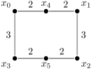
Figure 1. The augmented metric space $(M,d,f)$ of Example 3.13, with $f(x_{i})=i$. These are six points $\{x_{0},\dots,x_{5}\}$ in the plane, where the distances are given by the numbers next to each line.

Figure 2. The persistent set $S\colon P\to\mathsf{Set}$ of Example 3.13 obtained by taking the density-Rips persistence set of Fig. 1 and removing $x_{4}$ and $x_{5}$. Each node in the grid represents a partition of the $x_{i}$, where $x_{i}$ and $x_{j}$ are in the same partition if they are not separated by a line. The arrows are the functions that send the partition of $x_{i}$ in one node to the partition of $x_{i}$ in the other.

We claim that the persistence module $\mathcal{L}S\colon P\to\mathsf{Vec}$ decomposes into four summands, all of them interval modules. We denote these summands by $I_{0},I_{1},I_{2}$ and $I_{3}$, where each $I_{i}$ is associated to the generator $(p_{i},x_{i})$ of $S$, where $p_{i}=(0,i)\in P$. For each $i=0,\dots,3$, we set $(I_{i})_{p}=0$ for any $p<p_{i}$ and $(I_{i})_{p_{i}}=K$, and we define $\iota_{i}\colon I_{i}\to\mathcal{L}S$ by

$$(\iota_{0})_{p_{0}}(1) =[x_{0}], (\iota_{1})_{p_{1}}(1) =[x_{1}]-[x_{0}],$$

$$(\iota_{2})_{p_{2}}(1) =[x_{2}]-[x_{1}], (\iota_{3})_{p_{3}}(1) =[x_{3}]-[x_{0}]+[x_{1}]-[x_{2}].$$

The support of each $I_{i}$ are the grades $p\geq p_{i}$ such that $((\mathcal{L}S)_{p_{i}\to p}\circ(\iota_{i})_{p_{i}})(1)$ is not zero. It can be seen that these maps induce a decomposition $\mathcal{L}S\cong I_{0}\oplus I_{1}\oplus I_{2}\oplus I_{3}$.

However, no subset of the generators other than $\{x_{1},x_{2},x_{3}\}$ is rooted because each of the connected components given by $\{x_{1},x_{0}\}$, $\{x_{1},x_{2}\}$, $\{x_{2},x_{3}\}$, and $\{x_{0},x_{3}\}$ appear in $S$.

4. Rooted generators as a generalization of the elder rule

Single-parameter case.

We now suppose that the poset $P$ is a finite totally ordered poset. In this setting, the theory of rooted generators allows us to recover the elder rule [24] (see also [22] and [14]).

Proposition 4.1.

Let $P$ be a finite totally ordered poset and let $S\colon P\to\mathsf{Set}$ be a persistent set. Suppose that $S$ has at least two generators and that $S_{\top}$ is a singleton, where $\top$ is the maximum element of $P$. Then every maximal generator (in the preorder of Definition 3.1) is rooted.

Proof.

Let $x\in S_{p_{x}}$ be a maximal generator, and define

$$I_{x}\coloneqq\{q\in P\nonscript\>|{}\allowbreak{}\nonscript\>\mathopen{}\text{$q\geq p_{x}$ and, for any other generator $w\in S_{p_{w}}$, $S_{p_{w}\to q}(w)\neq S_{p_{x}\to q}(x)$}\}.$$

Since $p_{x}\in I_{x}$, $I_{x}$ is not empty, and we can consider the set $U\subset P$ of upper bounds of $I_{x}$. Moreover, since $S_{\top}=\{*\}$ and there are at least two generators by assumption, the set $U\setminus I_{x}$ is not empty. Let $\alpha$ be the least element in $U\setminus I_{x}$. By construction of $I_{x}$ and $U\setminus I_{x}$, there is a generator $y\in S_{p_{y}}$ such that $S_{p_{y}\to\alpha}(y)=S_{p_{x}\to\alpha}(x)$. Now, since $x$ is maximal, it holds that $p_{y}\leq p_{x}$, and we can define an idempotent $\varphi\colon S\to S$ by $\varphi_{p_{x}}(x)=S_{p_{y}\to p_{x}}(y)$, and $\varphi_{p_{z}}(z)=z$ for any other generator $z\in S_{p_{z}}$. Such an idempotent is well-defined by the way we have defined $\alpha$: if there is any other generator $w\in S_{p_{w}}$ such that $S_{p_{w}\to q}(w)=S_{p_{x}\to q}(x)$ then $\alpha\leq q$ and also $S_{p_{y}\to q}(y)=S_{p_{x}\to q}(x)$. We conclude that $x$ is rooted, as desired. ∎

Thus, when $P$ is a total order, we can decompose any persistence module $\mathcal{L}S$ by peeling off rooted generators, following Theorem 3.6 and by iteratively considering maximal generators.

Relation to constant conquerors.

Let $(M,d,f)$ be an augmented metric space. Cai, Kim, Mémoli and Wang [14] define the concept of a constant conqueror as follows. First, define an ultrametric on $M$: $u(x,x^{\prime})\coloneqq\min\{\varepsilon\in[0,\infty)\nonscript\>|{}\allowbreak{}\nonscript\>\mathopen{}\text{$x$ and $x^{\prime}$ are path-connected in $\mathcal{G}_{\varepsilon}(M)$}\}$.

Now fix a total order $\prec$ on $M$ and let $x\in M$ be a non-minimal element with respect to this order. A conqueror of $x$ in $M$ is another point $x^{\prime}\in M$ such that (1) $x^{\prime}\prec x$, and (2) for any $x^{\prime\prime}$ with $x^{\prime\prime}\prec x$ one has $u(x,x^{\prime})\leq u(x,x^{\prime\prime})$. Given a function $f\colon M\to\mathbb{R}$, a conqueror function of a non-minimal $x\in M$, with respect to $\prec$, is a function $c_{x}\colon[f(x),\infty)\to M$ that sends each $\sigma$ to a conqueror of $x$ in $M_{\sigma}$. For the minimal element $\bot$ of $M$ we define $c_{\bot}\colon[f(\bot),\infty)\to M$ to be the constant function at $\bot$.

Also, in the same paper [14], given a point $x\in M$, and assuming that $f\colon M\to\mathbb{R}$ is injective, the authors define the staircode of $x$ as the set given by

$$I_{x}\coloneqq\{(\varepsilon,\sigma)\in\mathbb{R}_{\geq 0}\times\mathbb{R}\nonscript\>|{}\allowbreak{}\nonscript\>\mathopen{}x\in M_{\sigma}\text{ and $x$ is the oldest in $[x]_{(\varepsilon,\sigma)}$}\},$$

where $[x]_{(\varepsilon,\sigma)}$ is the set of points that are path-connected to $x$ in $\mathcal{G}_{\varepsilon}(M_{\sigma})$ and being the “oldest” means $f(x)<f(x^{\prime})$ for any other $x^{\prime}\in[x]_{(\varepsilon,\sigma)}$. The authors also define an analogous notion when $f$ is not injective, which we do not reproduce here.

Finally, the authors ask the following question:

Question 4.2.

Let $(M,d,f)$ be an augmented metric space. If $x\in M$ has a constant conqueror function, is the interval module supported by $I_{x}$ a summand of its density-Rips persistence module?

If we replace constant conqueror by rooted generator then the answer is yes, by Corollary 3.7. The next example shows that the same cannot hold as originally stated in the question above.

Example 4.3.

Consider the subset $M$ of $\mathbb{R}$ given by the points $x_{0}=0$, $x_{1}=7.5$, $x_{2}=3$ and $x_{3}=5$. Under the metric induced by the Euclidean distance on $\mathbb{R}$, $M$ is a metric space, and can be made into an augmented metric space by defining $f(x_{i})=i$, see Fig. 3.

Figure 3. The augmented metric space $(M,d,f)$ of Example 4.3, with $M\subset\mathbb{R}$ and $f(x_{i})=i$.

Figure 4. We picture the density-Rips persistent set of Fig. 3.

Consider the only total order $\prec$ on $M$ compatible with $f$, $x_{0}\prec x_{1}\prec x_{2}\prec x_{3}$. The point $x_{1}$ has a constant conqueror: $x_{0}$ is the only candidate, and it is clear that, for every $i=1,\dots,3$ and $x^{\prime}\prec x_{1}$, $u_{i}(x_{1},x_{0})\leq u_{i}(x_{1},x^{\prime})$, where $u_{i}$ is the ultrametric of $M_{i}$, precisely because $x_{0}$ is the only point that satisfies $x^{\prime}\prec x_{1}$.

Let $S\colon P\to\mathsf{Set}$ be the density-Rips persistent set constructed from the augmented metric space $(M,d,f)$. Here, the poset $P$ is the subposet of $\mathbb{R}^{2}$ given by the grid $\{0,2,2.5,3,4.5,7.5\}\times\{0,1,2,3\}$, where the first coordinate represents the distances and the second coordinate the densities. We picture $S$ in Fig. 4. Now we proceed to decompose $\mathcal{L}S$. First, note that $x_{3}$ is a rooted generator, and consider an associated idempotent $\varphi\colon S\to S$. By Theorem 3.6, there is an interval $I\coloneqq\operatorname{img}(\mathrm{id}_{\mathcal{L}S}-\mathcal{L}\varphi)$ in the decomposition, and we can continue considering the persistent set $\operatorname{img}\varphi$. In $\operatorname{img}\varphi$, $x_{0}$ is a minimal generator. By Theorem 3.11 (and its proof) there is an idempotent $\psi\colon\operatorname{img}\varphi\to\operatorname{img}\varphi$ such that $I^{\prime}\coloneqq\operatorname{img}\mathcal{L}\psi$ is an interval. Applying Theorem 3.6 again, we obtain a decomposition of $\mathcal{L}S$ of the form

$$I\oplus I^{\prime}\oplus\operatorname{img}(\mathrm{id}_{\mathcal{L}\operatorname{img}\varphi}-\mathcal{L}\psi).$$

By direct computation, it can be seen that $\operatorname{img}(\mathrm{id}_{\mathcal{L}\operatorname{img}\varphi}-\mathcal{L}\psi)$ is isomorphic to the persistence module described in Fig. 5. Moreover, this persistence module is indecomposable, which can be checked by looking at its endomorphisms: a persistence module $F$ is indecomposable if and only if every endomorphism of $F$ is either nilpotent or an isomorphism (see [9], and [10]).

Figure 5. An indecomposable persistence module $F\colon P\to\mathsf{Vec}$, as referenced in Example 4.3.

Note that $x_{1}$ is not a rooted generator in $\mathcal{L}S$. In $M_{1}$, $x_{1}$ is its own connected component during $\varepsilon\in[0,7.5)$, until $x_{0}$ joins the connected component. And in $M_{3}$ it is by itself during $\varepsilon\in[0,2.5)$ and then joins the connected component of $x_{3}$, which is not connected to $x_{0}$ at that point. Similarly, $x_{2}$ is not rooted.

Remark 4.4.

Note that in Condition (2) of the definition of conqueror, we require that $x^{\prime\prime}\prec x$. This requirement measures part of the difference between constant conqueror function and rooted generator for augmented metric spaces. If we drop this requirement, denoting the resulting concept by conqueror^∗, we suppose that $f$ is injective, and that $\prec$ is compatible with the order induced by $f$, then a non-minimal, with respect to $\prec$, point $x\in M$ has a constant conqueror^∗ function if and only if $x$ is a rooted generator, as in Proposition 3.4.

5. A lower bound on the number of expected intervals

We apply the theory we have developed to the study of how a typical decomposition of a persistence module coming from density-Rips might look like. In particular, suppose we sample independently $n$ points from a common density function $f(x)$ in $\mathbb{R}^{d}$, obtaining a finite metric space $M\subset\mathbb{R}^{d}$. We can then consider the augmented metric space $(M,d,f)$, where $f$, rather than being an estimated density, is the true underlying density function. This setting resembles actual practice, but is more suitable to theoretical study. Let $S$ be the density-Rips persistent set of $M$. Then, how many intervals can we expect in the decomposition of $\mathcal{L}S$? The following theorem says that, under very general conditions on $f$, regardless of $d$, and as $n$ goes to infinity, we can at least expect $25\%$ of the summands to be intervals.

Theorem 5.1.

Let $X_{1},\dots,X_{n}$ be i.i.d. points taking values in $\mathbb{R}^{d}$, sampled from a common density function $f(x)$ that is continuous almost everywhere with respect to the Lebesgue measure.

Consider the finite augmented metric space $(M=\{X_{1},\dots,X_{n}\},d_{M},f)$, where $d_{M}$ is induced by the Euclidean metric in $\mathbb{R}^{d}$, and let $S$ be its density-Rips persistent set.

Let $\mathfrak{I}_{n}$ be the random variable that counts the number of intervals in the indecomposable decomposition of $\mathcal{L}S$, and let $\mathfrak{S}_{n}$ be the random variable that counts the total number of summands in the same decomposition. We have

$$\liminf_{n\to\infty}\operatorname{E}\left[\frac{\mathfrak{I}_{n}}{\mathfrak{S}_{n}}\right]\geq c(d),$$ (3)

where $c(d)$ is a constant that depends on $d$, and $c(1)=\frac{1}{3}$, $c(2)\approx 0.31$ and $c(d)\downarrow\frac{1}{4}$ as $d\to\infty$.

The rest of the section is dedicated to proving this theorem. The nearest neighbor graph of a metric space plays a fundamental role.

Definition 5.2.

The nearest neighbor graph of $M$ is the directed graph on $M$ given by the directed edges of the form $(x,x^{\prime})$, where $x^{\prime}$ is the nearest neighbor of $x$.

Now, we are interested in estimating the number of neighborly rooted elements, as in Definition 3.8, as they induce an interval in the decomposition of $\mathcal{L}S$. However, in general being neighborly rooted depends on $f$. To do without the condition on $f$ we have:

Lemma 5.3.

Let $(M,d_{M},f)$ be an augmented metric space and let $S$ be its density-Rips persistent set. There are at least as many intervals in the indecomposable decomposition of $\mathcal{L}S$ as $2$-cycles in the nearest neighbor graph of $M$.

Proof.

We can assume without loss of generality that $\lvert M\rvert\geq 2$. Let $G$ be the nearest neighbor graph of $M$. The only cycles in this graph are precisely the 2-cycles, and each weakly connected component of $G$ contains exactly one 2-cycle (see [25]).

Let $C_{1},\dots,C_{k}$ be the weakly connected components of $G$. Fix $i\in\{1,\dots,k\}$, and let $x,y\in M$ be such that $(x,y)$ and $(y,x)$ is the 2-cycle in $C_{i}$. Either $f(y)\leq f(x)$ or $f(x)\leq f(y)$, and either $x$ is neighborly rooted, $y$ is neighborly rooted, or both are neighborly rooted. Say $x$ is neighborly rooted, and define an endomorphism $\varphi_{i}\colon S\to S$ by setting

$$(\varphi_{i})_{p_{z}}(z)=\begin{cases}S_{p_{y}\to p_{x}}(y),&\text{if $x=z$,}\\ z,&\text{otherwise,}\end{cases}$$

for every generator $z\in S_{p_{z}}$. Such an endomorphism is well-defined as shown in Proposition 3.4.

Constructing, for each $i$, an idempotent $\varphi_{i}$ as above, it is clear that we can iteratively peel off the associated intervals, yielding the desired conclusion. ∎

Naturally, the number of 2-cycles is half the number of points that are the nearest neighbor of its nearest neighbor. The problem of estimating the probability for a point to be the nearest neighbor of its nearest neighbor, assuming a random point process, has been studied by multiple authors (see [36, 26, 27, 21, 25]).

In our case, when we have $X_{1},\dots,X_{n}$ i.i.d. points in $\mathbb{R}^{d}$ sampled from a common density function $f$ under the conditions of Theorem 5.1, by [27, Theorem 1.1], and letting $N_{i,n}$ denote the probability event that $X_{i}$ is the nearest neighbor of its nearest neighbor, we have

$$\lim_{n\to\infty}\operatorname{P}(N_{i,n})=b(d),$$ (4)

where $b(d)$ is the volume of a unit $d$-sphere divided by the volume of the union of two unit spheres with centers at distance $1$. In fact, $b(1)=\frac{2}{3}$, $b(2)\approx 0.621$, and $b(d)\downarrow\frac{1}{2}$ as $d\to\infty$ (see [36, Table 2]), and we define $c(d)\coloneqq\frac{b(d)}{2}$.

We are now ready to finish the proof of Theorem 5.1 at the start of the section. Applying Lemma 5.3 and the linearity of expectation, it holds

$$\operatorname{E}[\mathfrak{I}_{n}]\geq\operatorname{E}\left[\sum_{i=1}^{n}\frac{I(N_{i,n})}{2}\right]=\sum_{i=1}^{n}\frac{\operatorname{E}[I(N_{i,n})]}{2}=\sum_{i=1}^{n}\frac{\operatorname{P}(N_{i,n})}{2},$$

where $I(N_{i})$ is the indicator random variable of $N_{i,n}$. By Eq. 4 we have

$$\liminf_{n\to\infty}\operatorname{E}\left[\frac{\mathfrak{I}_{n}}{n}\right]\geq\frac{b(d)}{2}=c(d).$$

Finally, noting that the number of summands in the decomposition is bounded by the number of points, $\mathfrak{S}_{n}\leq n$, by the lemma below, Eq. 3 of Theorem 5.1 follows, finishing the proof.

Lemma 5.4.

Let $(M,d_{M},f)$ be an augmented metric space, and let $S\colon P\to\mathsf{Set}$ be its density-Rips persistent set. Then any decomposition of $\mathcal{L}S$ consists of at most $n=\lvert M\rvert$ summands.

Proof.

Given a persistence module $F\colon P\to\mathsf{Vec}$, denote by $\beta_{0}(F)\colon P\to\mathbb{N}$ the function that assigns to each $p\in P$ the multigraded $0$-th Betti number of $F$ at $p\in P$ (we refer to [30] for their definition). Precisely because $S$ has $n$ generators, it is not hard to see that $\sum_{p\in P}\beta_{0}(\mathcal{L}S)(p)=n$.

Consider a decomposition $\mathcal{L}S\cong X_{1}\oplus\cdots\oplus X_{k}$. Since Betti numbers are additive, we have $\beta_{0}(\mathcal{L}S)=\sum_{i=1}^{k}\beta_{0}(X_{i})$. Therefore, we can write

$$\sum_{p\in P}\beta_{0}(\mathcal{L}S)(p)=\sum_{i=1}^{k}\sum_{p\in P}\beta_{0}(X_{i})(p)=n.$$ (5)

Now, since $\sum_{p\in P}\beta(X_{i})(p)\geq 1$ if $X_{i}\neq 0$, it follows that $k\leq n$. ∎

6. Discussion

Although we have focused our attention to augmented metric spaces and density-Rips, rooted subsets can be applied to other persistent sets. Of special interest for us is the degree-Rips filtration [5] of a metric space, where we filter by the degree of the vertices in the underlying geometric graphs. To accommodate this situation, one could modify condition 1 of Proposition 3.4 to take into account the evolution of the degrees, rather than the density. We leave an in-depth treatment of this case for future work.

We have seen, both in our lower bound of Section 5 and in preliminary experimental evaluation, that we can expect to find many intervals in the decomposition of those persistence modules coming from geometry, at least in the cases considered here. This is in contrast to the purely algebraic setting, where, in light of recent developments [2, 3], looking for a decomposition might fall short.

References

- [1] Hideto Asashiba, Mickaël Buchet, Emerson G. Escolar, Ken Nakashima, and Michio Yoshiwaki, On interval decomposability of 2D persistence modules, Computational Geometry 105/106 (2022), Paper No. 101879, 33, doi:10.1016/j.comgeo.2022.101879.
- [2] Ulrich Bauer, Magnus B. Botnan, Steffen Oppermann, and Johan Steen, Cotorsion torsion triples and the representation theory of filtered hierarchical clustering, Advances in Mathematics 369 (2020), 107171, 51, doi:10.1016/j.aim.2020.107171.
- [3] Ulrich Bauer and Luis Scoccola, Generic two-parameter persistence modules are nearly indecomposable, November 2022, arXiv:2211.15306.
- [4] Håvard Bakke Bjerkevik, Magnus Bakke Botnan, and Michael Kerber, Computing the interleaving distance is NP-hard, Foundations of Computational Mathematics 20 (2020), no. 5, 1237–1271, doi:10.1007/s10208-019-09442-y.
- [5] Andrew J. Blumberg and Michael Lesnick, Stability of 2-parameter persistent homology, Foundations of Computational Mathematics (2022), doi:10.1007/s10208-022-09576-6.
- [6] Magnus Bakke Botnan and William Crawley-Boevey, Decomposition of persistence modules, Proceedings of the American Mathematical Society 148 (2020), no. 11, 4581–4596, doi:10.1090/proc/14790.
- [7] Magnus Bakke Botnan and Michael Lesnick, Algebraic stability of zigzag persistence modules, Algebraic & Geometric Topology 18 (2018), no. 6, 3133–3204, doi:10.2140/agt.2018.18.3133.
- [8] Magnus Bakke Botnan, Steffen Oppermann, Steve Oudot, and Luis Scoccola, On the bottleneck stability of rank decompositions of multi-parameter persistence modules, July 2022, arXiv:2208.00300.
- [9] Michel Brion, Representations of quivers, Geometric methods in representation theory. I, Sémin. Congr., vol. 24, Soc. Math. France, Paris, 2012, pp. 103–144.
- [10] Jacek Brodzki, Matthew Burfitt, and Mariam Pirashvili, On the complexity of zero-dimensional multiparameter persistence, August 2020, arXiv:2008.11532.
- [11] Mickaël Buchet, Frédéric Chazal, Tamal K. Dey, Fengtao Fan, Steve Y. Oudot, and Yusu Wang, Topological Analysis of Scalar Fields with Outliers, 31st International Symposium on Computational Geometry, LIPIcs. Leibniz Int. Proc. Inform., vol. 34, 2015, pp. 827–841, doi:10.4230/LIPIcs.SOCG.2015.827.
- [12] Mickaël Buchet and Emerson G. Escolar, Every 1D persistence module is a restriction of some indecomposable 2D persistence module, Journal of Applied and Computational Topology 4 (2020), no. 3, 387–424, doi:10.1007/s41468-020-00053-z.
- [13] Mickaël Buchet and Emerson G. Escolar, Realizations of indecomposable persistence modules of arbitrarily large dimension, Journal of Computational Geometry 13 (2022), no. 1, 298–326, doi:10.20382/jocg.v13i1a12.
- [14] Chen Cai, Woojin Kim, Facundo Mémoli, and Yusu Wang, Elder-rule-staircodes for augmented metric spaces, SIAM Journal on Applied Algebra and Geometry 5 (2021), no. 3, 417–454, doi:10.1137/20M1353605.
- [15] Gunnar Carlsson and Facundo Mémoli, Characterization, stability and convergence of hierarchical clustering methods, Journal of Machine Learning Research 11 (2010), 1425–1470.
- [16] by same author, Multiparameter hierarchical clustering methods, Classification as a tool for research, Stud. Classification Data Anal. Knowledge Organ., Springer, Berlin, 2010, pp. 63–70, doi:10.1007/978-3-642-10745-0\_6.
- [17] Gunnar Carlsson and Facundo Mémoli, Classifying Clustering Schemes, Foundations of Computational Mathematics 13 (2013), no. 2, 221–252, doi:10.1007/s10208-012-9141-9.
- [18] Gunnar Carlsson and Afra Zomorodian, The Theory of Multidimensional Persistence, Discrete & Computational Geometry 42 (2009), no. 1, 71–93, doi:10.1007/s00454-009-9176-0.
- [19] Kenneth L. Clarkson, Fast algorithms for the all nearest neighbors problem, 24th Annual Symposium on Foundations of Computer Science, IEEE, 1983, pp. 226–232, doi:10.1109/SFCS.1983.16.
- [20] Anne Collins, Afra Zomorodian, Gunnar Carlsson, and Leonidas J. Guibas, A barcode shape descriptor for curve point cloud data, Computers & Graphics 28 (2004), no. 6, 881–894, doi:10.1016/j.cag.2004.08.015.
- [21] Trevor F. Cox, Reflexive nearest neighbours, Biometrics 37 (1981), no. 2, 367, doi:10.2307/2530424.
- [22] Justin Curry, The fiber of the persistence map for functions on the interval, Journal of Applied and Computational Topology 2 (2018), no. 3-4, 301–321, doi:10.1007/s41468-019-00024-z.
- [23] Tamal K. Dey and Cheng Xin, Generalized persistence algorithm for decomposing multiparameter persistence modules, Journal of Applied and Computational Topology 6 (2022), no. 3, 271–322, doi:10.1007/s41468-022-00087-5.
- [24] Herbert Edelsbrunner and John L. Harer, Computational topology: an introduction, American Mathematical Society, Providence, RI, 2010, doi:10.1090/mbk/069.
- [25] David Eppstein, Michael S. Paterson, and Frances F. Yao, On nearest-neighbor graphs, Discrete & Computational Geometry 17 (1997), no. 3, 263–282, doi:10.1007/PL00009293.
- [26] Norbert Henze, On the probability that a random point is the j th nearest neighbour to its own k th nearest neighbour, Journal of Applied Probability 23 (1986), no. 1, 221–226, doi:10.2307/3214132.
- [27] by same author, On the fraction of random points by specified nearest-neighbour interrelations and degree of attraction, Advances in Applied Probability 19 (1987), no. 4, 873–895, doi:10.2307/1427106.
- [28] Jon Kleinberg, An impossibility theorem for clustering, Advances in Neural Information Processing Systems, vol. 15, MIT Press, 2002.
- [29] Michael Lesnick and Matthew Wright, Interactive visualization of 2-d persistence modules, December 2015, arXiv:1512.00180.
- [30] by same author, Computing minimal presentations and bigraded Betti numbers of 2-parameter persistent homology, SIAM Journal on Applied Algebra and Geometry 6 (2022), no. 2, 267–298, doi:10.1137/20M1388425.
- [31] Saunders Mac Lane, Categories for the working mathematician, Graduate Texts in Mathematics, vol. 5, Springer New York, 1978, doi:10.1007/978-1-4757-4721-8.
- [32] Leland McInnes and John Healy, Accelerated hierarchical density clustering, 2017 IEEE International Conference on Data Mining Workshops, 2017, pp. 33–42, doi:10.1109/ICDMW.2017.12.
- [33] Samantha Moore, Hyperplane restrictions of indecomposable -dimensional persistence modules, Homology, Homotopy and Applications 24 (2022), no. 2, 291–305, doi:10.4310/HHA.2022.v24.n2.a14.
- [34] Alexander Rolle and Luis Scoccola, Persistable: Persistent and stable clustering, URL: https://github.com/LuisScoccola/persistable.
- [35] by same author, Stable and consistent density-based clustering, July 2021, arXiv:2005.09048.
- [36] Mark F. Schilling, Mutual and shared neighbor probabilities: finite- and infinite-dimensional results, Advances in Applied Probability 18 (1986), no. 2, 388–405, doi:10.2307/1427305.
- [37] Bernard W. Silverman, Density estimation for statistics and data analysis, Monographs on Statistics and Applied Probability, Chapman & Hall, London, 1986.
- [38] Pravin M. Vaidya, An algorithm for the all-nearest-neighbors problem, Discrete & Computational Geometry 4 (1989), no. 2, 101–115, doi:10.1007/BF02187718.