Aftermath epidemics: Percolation on the sites visited by generalized random walks

Abstract

We study percolation on the sites of a finite lattice visited by a generalized random walk of finite length with periodic boundary conditions. More precisely, consider Levy flights and walks with finite jumps of length $>1$ (like Knight’s move random walks (RWs) in two dimensions and generalized Knight’s move RWs in 3D). In these walks, the visited sites do not form (as in ordinary RWs) a single connected cluster, and thus percolation on them is nontrivial. The model essentially mimics the spreading of an epidemic in a population weakened by the passage of some devastating agent – like diseases in the wake of a passing army or of a hurricane. Using the density of visited sites (or the number of steps in the walk) as a control parameter, we find a true continuous percolation transition in all cases except for the 2D Knight’s move RWs and Levy flights with Levy parameter $\sigma\geq 2$. For 3D generalized Knight’s move RWs, the model is in the universality class of pacman percolation, and all critical exponents seem to be simple rationals, in particular $\beta=1$. For 2D Levy flights with $0<\sigma<2$, scale invariance is broken even at the critical point, which leads at least to very large corrections in finite-size scaling, and even very large simulations were unable to unambiguously determine the critical exponents.

I Introduction

One disaster often does not come alone. In the present paper we deal with the purely geometric – i.e., percolation – aspects of an epidemic which comes in the wake of another disaster like a hurricane or a war Smallman , and can spread only on the sites weakened by the first.

Percolation in its simplest version (called OP in the following) deals with the establishment of long range connectivity in random but statistically homogeneous systems with only short range links between its units Stauffer ; Sahimi . The two best known examples of OP are site and bond percolation, where the system is a regular lattice of finite dimension, and local links are established by inserting sites or bonds Stauffer .

This is one of the paradigmatic models in statistical physics and has many applications, the most important one being the spreading of epidemics Bailey . Starting from a local seed, a system-wide epidemic (or pandemic) can evolve only, if the spreading agent (virus, bacterium, or even rumor) can reach wide regions, i.e., if large clusters of sites are connected. If the population is originally healthy and susceptible (except for the seed), and becomes immune or dead after a finite time of illness, this is the so-called SIR (susceptible-infected-removed) model Kermack ; Grassberger1983 .

There are of course many modifications of this simple scenario Saberi ; Araujo :

– The system is not a regular lattice, but some sort of network Newman ; referee2-1 ; referee2-2 . This leads to new universality classes, but at least if the network is close to regular (all nodes have similar degree) and uncorrelated, the situation is similar as to a regular lattice.

– When recovered individuals become susceptible again, the resulting SIS model is in a different universality class from SIR or OP Hinrichsen .

– If there are finite incubation or latency periods between exposure to the spreading agent and the development of symptoms, in the resulting SEIR (susceptible-exposed-infectious-removed) compartmental model Bailey ; referee1-1 the universality class is in general not changed.

– Things change again, if contact with more than one infectious neighbor is needed to infect a susceptible individual. In the extreme case of bootstrap and $k$-core percolation Adler ; di_Muro , clusters can grow (or do not shrink) only, if new (old) sites have a certain minimal number of neighbors in the cluster. This can be relaxed so infection of a new site is more likely if it has more infected neighbors Janssen ; Bizhani ; Dorogovtsev2006 . The most dramatic effect in such cases is that the percolation transition can become discontinuous or, actually, hybrid: Although the order parameter jumps at the transition point, one also observes scaling laws as for continuous transitions.

– Similar cooperativity effects occur, if two (or more) diseases cooperate in the sense that infection by one also makes the individual more susceptible to be infected by the other Cai .

– Very important, in particular in modern times where people can carry infections over very long distances by flights, are nonlocal single links. Often, this is modeled by assuming that the infectious agent can perform a Levy flight, i.e., the probability for a link between two sites is described by a power law Grassberger1986 ; Janssen ; Linder ; Grassberger2012 ; Grassberger2013 ; Gori . In this case one finds continuous transitions in new universality classes which depend on the value of the power-law exponent.

– While long-range effects are treated in the above models as long-range contacts between static individuals, more realistic models take into account that individuals can move referee1-2 ; Belik . In this case the connection with percolation is, strictly spoken, lost, because there is no static infected cluster when the epidemic has ended. If the movements are slow, this may not be a big problem and the standard scaling laws could still hold with minor adaptions, but in case of Levy flights all scaling laws have to be re-considered referee1-2 ; Belik .

– In OP, new local connections are established randomly. In contrast, in explosive percolation Achlioptas ; Christensen (EP) one inserts new connections such that the occurrence of large clusters is delayed. The percolation transitions in EP were first thought to be discontinuous, but they are actually continuous. Apart from the smallness of the order parameter exponent $\beta$, its most striking feature is that for finite lattice sizes $L$, the width of the critical region and its shift relative to the infinite lattice critical point satisfy power laws with different exponents Bizhani – at least when analyzed in the conventional way where the transition point is defined as independent of the individual realization of the process Li2023 .

– The system can be non-homogeneous in the sense that some regions are more susceptible and others less so. This can lead to multiple percolation transitions, such that changes in cluster size are of order $N$ in each, where $N$ is the size of the system Bianconi .

– Even if the system is homogeneous on large scales, it might be that there are long-range correlations between the densities of susceptible individuals and/or the links. This is called correlated percolation (CP), and is maybe the largest and most varied class of nontrivial percolation models Correlated Percolation referee2 .

It is this class of models which is considered in the present paper.

By far the best studied special case is the Ising model. It is well known that the Ising critical point can be understood as a percolation type transition for carefully defined (Fortuin-Casteleyn) clusters Fortuin . But one can also study the percolation of clusters defined simply as connected sets of + and - spins, and of the boundaries between them. This was recently done by Grady Grady , who found in three dimensions a true percolation transition which is not in the OP universality class. Remarkably, Grady found that, as in EP, the width of the critical region for finite $L$ and its shift from the exact critical point at $L=\infty$ scale with different exponents.

Another class of CP models is one where the correlations are assumed to decay with power laws $C(r)\sim r^{-\alpha}$, without specifying the mechanism which generated them Weinrib-Halperin ; Weinrib ; Schrenk . Whether the resulting percolation transition is in the OP class or not should now depend on $\alpha$, according to a generalized Harris criterion: The universality class should be modified iff $d\nu^{(0)}>\alpha$, where $\nu^{(0)}$ is the correlation length exponent of the model without long-range correlations. This is seen in Ref. Schrenk for some critical exponents, but not for all.

Finally, there is pacman percolation Abete ; Kantor . In this case, all sites are susceptible initially. But before the actual percolation process starts, a random walker performs a walk (with periodic boundary conditions) of $T$ steps, where $T\sim N$, with $N=L^{d}$ being the number of sites. Percolation is then considered only on those sites which were not visited by the walker.

The model studied in the present paper can be seen as the opposite of pacman percolation: We again have a finite-time random walk (RW) before the percolation proper takes place, but now the percolation process can take place only on sites that had been visited by the walker. A real-world scenario which might be modeled by this is an army or a hurricane that passes through some geographic region, and an epidemic which can evolve only in the areas devastated by them. It is true that hurricanes in the Caribbean don’t make RWs, but Timur’s armies in Iran and neighboring countries Timur and the armies in the Thirty years War in Germany Germany came very close. Periodic boundary conditions are used both for the walker and for the percolation process.

An immediate problem with such a type of models is that the visited sites are connected for an ordinary RW, and thus the problem of percolation seems trivial. The way out of this dilemma is, of course, to modify the walk such that visited sites are not (necessarily) connected. In the present paper, we study two such modifications:

(a) Knight’s move and next-nearest neighbor (NNN) move RW. A Knight’s move in chess is one where one moves two lattice constants in one direction (say, x), and one in the other (say, y). From a given position, there are eight such moves. A NNN move RWs (NNN-RW) is a walk where one moves $\pm 1$ step in each direction. In the following, we shall only show results for the Knight’s move RW, but we have also done extensive simulations for NNN-RWs. We will show that there is no sharp percolation transition in this model in two dimensions, but there is one if the model is generalized to 3D. A Knight’s move in this generalized 3D walk is one where one moves two lattice constants in one direction and one in each of the two others. In this case there are 24 moves.

(b) Levy flights. Here, the probability for a step to have a length $>r$ decreases for large $r$ as

$$P(r)\sim r^{-\sigma}$$ (1)

with $0<\sigma<2$. Here, we studied only two dimensional lattices. For $\sigma\to 0$, the walk is just a sequence of random jumps, and our model reduces to site percolation. For $\sigma>2$, the walk is in most respects equivalent to a RW, except that visited sites do not necessarily form a single connected cluster. It is for the latter reason that we also studied the case $\sigma=2.5$, to verify that the behavior is the same as for the Knight’s move RW. We also studied the case $\sigma=2$, which is at the border between Levy flights and ordinary walks.

A particular feature of the present model is that the finite value of $T$ can induce, for finite $L$, an additional characteristic length scale. For RWs, this length scale would be the square root of the rms end-to-end distance

$$\sqrt{\langle R^{2}}\rangle\sim T^{1/2}\sim L^{d/2},$$ (2)

which diverges for $d>2$ faster than $L$ when $L\to\infty$, if the periodic boundary conditions would not bring it down to $L$. Indeed, as shown in Ref. Kantor , the latter implies that the correlation between visited sites decays as $C(r)\sim r^{2-d}$. For Levy flights, different powers of $R$ scale differently, $\langle R^{q}\rangle\sim T^{q/\sigma}$, if $q>\sigma$ Mandelbrot , and the correlation function $C(r)$ is, in general, not a power law (see Appendix). Thus it is not scale-free, suggesting that several new length scales might be involved. This might imply that the standard finite size scaling (FSS) behavior is no longer valid for Levy flights, and that, in particular, the width and the shift of the critical peak in variables like the fluctuations of the order parameter might scale with different exponents, as found also in EP Christensen and in boundary percolation in the Ising model Grady .

II Definitions of the models, algorithms, and computational details

Both models live on square, respectively, cubic lattices. For computational efficiency, we replaced the periodic boundary conditions by helical ones, where one uses a single integer to label sites and neighbors of site $i$ are $(i\pm 1)\;{\rm mod}\;N,(i\pm L)\;{\rm mod}\;N,\ldots(i\pm L^{d})\;{\rm mod}\;N$. For generating Levy flights, we used the algorithm of Refs. Linder ; Grassberger2013 : First, two random numbers ($\delta x,\delta y$) between 0 and 1 are chosen randomly. If $r^{2}\equiv\delta x^{2}+\delta y^{2}\geq 1$, they are discarded and a new pair is chosen. OtheRWsise, $\Delta x=\pm\frac{\delta x}{r^{1+2/\sigma}}$ and $\Delta y=\pm\frac{\delta y}{r^{1+2/\sigma}}$, where all four sign combinations are chosen with equal probability.

In the following, we shall use the words walk and walker both for Levy walks and for (generalized) Knight’s move walks.

In the Introduction, walk and percolation were discussed as independent and subsequent parts of the model, but for computational efficiency we measured the properties related to percolation already during the walk by means of the site insertion version of the Newman-Ziff (NZ) algorithm Newman-Ziff . In our algorithm, we keep track of the number $n$ of sites visited by the walker (we use $\rho=n/N$ as control parameter) and the size $S_{n}$ of the largest cluster when $n$ sites are visited ($S_{n}/N$ is used as order parameter). At each step of the walk we registered whether a new site was visited or not. In the latter case, the next step was taken immediately. If a new site $i$ was visited, however, we increased the number $n$ of visited sites by 1 and performed one step of the NZ algorithm. During this step, the connected cluster containing $i$ is determined. Let us call its size $C_{n}$, whence

$$S_{n}=\max\{S_{n-1},C_{n}\}.$$ (3)

The $n$th gap is defined as

$$\Delta_{n}=S_{n+1}-S_{n},$$ (4)

and the maximal gap over all values of $n$ is called $\Delta_{\rm max}$, while the $n$-value at which the maximum occurs is called $n_{\rm max}$ and the giant cluster size at this point is $S_{\rm max}$.

As observables we measured the average order parameter and its variance as functions of $n$, the averages of $\Delta_{\rm max}$ and $n_{\rm max}$, and their variances. These were measured at lattice sizes $L=32,64,\ldots 16384$ for $d=2$, and at $L=32,64,\ldots 512$ for $d=3$. The number of realizations for each Levy flight parameter $\alpha$ and for each dimension in the case of (generalized) Knight’s move RWs was $>70\,000$ for the largest $L$, and increased up to $>2\,000\,000$ for the smallest.

III Finite-size scaling

Because FSS might be different in the present model in view of the additional length scale induced by the finiteness of the walk time $T$, we should review the standard scenario for its scaling.

We expect that ${\rm Var}[S_{n}]$ has a peak near the percolation transition which gets sharper with increasing $N$. At the same values of $N$, the gaps should also be maximal. Let us call $\rho_{c}(L)$ the position of the peak of the distribution of $n_{\rm max}/N$ at given $N=L^{d}$, and $\rho_{c}=\lim_{L\to\infty}$. Let us furthermore define the order parameter exponent $\beta$ and the correlation length exponent $\nu$ by demanding for infinite systems that

$$s\equiv L^{-2}\langle S_{n}(\rho)\rangle\sim(\rho-\rho_{c})^{\beta}\quad{\rm for}\rho>\rho_{c}$$ (5)

and

$$\xi(\rho)\sim|\rho-\rho_{c}|^{-\nu}\;,$$ (6)

where $\xi(\rho)$ is the correlation length which for percolation is defined as the rms radius of the largest finite cluster.

Standard (FSS) arguments (mainly that observables are homogeneous functions near a critical point, that there is only one unique divergent length scale as $\rho\to\rho_{c}$, and that the scaling of a quantity depends only on its (anomalous) dimension, lead to the ansatzes

$$s=L^{d_{f}-d}\Psi_{S}[(\rho-\rho_{c})L^{1/\nu}]$$ (7)

and

$$\chi\equiv L^{-2}\{{\rm Var}[S_{n}(\rho)]\}^{1/2}=L^{d_{f}-d}\Psi_{\chi}[(\rho-\rho_{c})L^{1/\nu}],$$ (8)

where

$$d_{f}=d-\beta/\nu.$$ (9)

For bond percolation (whether correlated or not), $S_{n}$ would increase whenever the largest cluster eats a smaller one. The largest gap would thus occur when the largest second-largest cluster gets eaten. If we still assume that all masses scale with $L$ according to their anomalous dimension, this would imply that also

$$\langle\Delta_{\rm max}\rangle\sim\chi_{{}_{\Delta}}\;\equiv\;\{{\rm Var}[\Delta_{\rm max}]\}^{1/2}\sim L^{d_{f}}$$ (10)

at criticality, while equations analogous to Eqs. (7) and (8) (with scaling functions $\Psi_{\Delta}$ and $\Psi_{\chi_{{}_{\Delta}}}$) should hold for $\rho\neq\rho_{c}$.

For the present case of site percolation, essentially the same argument applies. There, $\Delta_{n}$ corresponds to the sum of a small number of eaten neighboring clusters, and Eq.(10) can be assumed still to hold.

Finally, we expect that distributions of observables like $S_{\rm max},\rho_{\rm max}$ (the density of visited sites where the largest gap occurs) and $\Delta_{\rm max}$ should be, up to normalization, functions of dimensionless variables, where we can write $S_{\rm max}/L^{d_{f}},(\rho-\rho_{c})L^{1/\nu}$ and $\Delta/L^{d_{f}}$, so that we can write

$$P_{S}(S_{\rm max})=L^{-d_{f}}f_{S}(S_{\rm max}/L^{d_{f}}),$$ (11)

$$P_{\rho}(\rho_{\rm max})=L^{1/\nu}f_{\rho}[(\rho_{\rm max}-\rho_{c})L^{1/\nu}]$$ (12)

and

$$P_{{}_{\Delta}}(\Delta_{\rm max})=L^{-d_{f}}f_{{}_{\Delta}}(\Delta_{\rm max}/L^{d_{f}})$$ (13)

(notice that Eqs. (11) and (13) of Ref. Fan , which are analogous to Eqs.(11) and (13) are more complicated without need).

According to the standard FSS scenario, the variance of $S_{n}$ and the distribution of $\rho_{\rm max}$ have near-by peaks which have the same scaling with $L$ and whose position is shifted from $\rho_{c}$ by the same scaling. If we denote the average of these two peak positions as $\rho_{c}(L)$, we should thus have

$$\rho_{c}(L)-\rho_{c}\sim{\rm peak}\;{\rm width}\sim L^{-1/\nu}.$$ (14)

IV Numerical Results

IV.1 Two dimensions

IV.1.1 Conventional variables

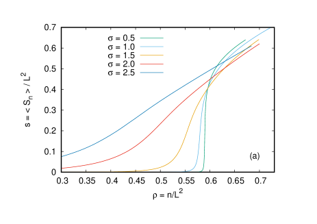
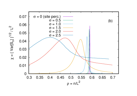
Figure 1: Order parameters (a) and the square root of their variances (b) at $L=16384$, for five values of $\sigma$ between 0 and 2.5, plotted against the density of allowed sites $\rho$ which serves as a control parameter.

We studied percolation on the sites visited by Levy flights with $\sigma=0.1,0.2,0.3,0.5,0.75,1.0,1.25,1.5,1.7$, $1.8,1.9,2.0$ and $2.5$. The last two values are strictly speaking no longer Levy flights (where $\sigma<2$ for $d=2$) but scale like ordinary RWs, but we also can use the Levy flight generating algorithm for these values, and get nontrivial results because the visited sites do not form, in general, connected clusters. We also simulated ordinary site percolation, which corresponds to $\sigma=0$, to see whether the scaling changes when going from $\sigma=0$ to $\sigma>0$.

In Fig. 1 we show the order parameter $s$ and its fluctuations $\chi$ as functions of the density $\rho$ of visited sites, for $N=16384$ and for typical values of $\sigma$. We see the very sharp transition for ordinary site percolation ($\sigma=0$), while the transitions become increasingly more fuzzy for increasing $\sigma$ and happen at smaller densities of allowed sites. Indeed we claim that the leftmost curve (for $\sigma=2.5$) and maybe also that for $\sigma=2$ do not show phase transitions at all. To settle this question, we also have to look at smaller $L$ and perform careful FSS analyses.

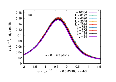
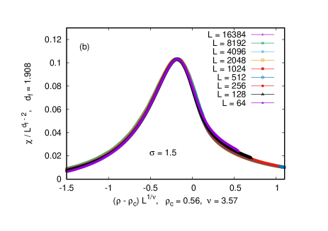
Figure 2: Data collapse plots of $\chi$ against $\rho$ for $\sigma=0$ (panel a) and $\sigma=1.5$ (panel b). The critical exponents used in these plots are the exact ones for standard OP in panel (a), and fitted ones in panel(b). Note that, in view of the visible deviations from a perfect data collapse in panel (a) (where the asymptotic scaling is known exactly), the good data collapse in panel (b) might be a bit fortuitous, and the precise values of the fitted exponents for $\sigma=1.5$ should not be taken too seriously.

In Fig. 2 we show the values of $\chi$ against $\rho$ for $L$ ranging from 64 to 16384, and for $\sigma=0$ (panel a) and $\sigma=1.5$ (panel b). More precisely, in view of Eq. (8), we plotted $L^{d-d_{f}}\chi$ against $(\rho-\rho_{c})L^{1/\nu}$, where we took the standard OP values of $d_{f}$ and $\nu$ for $\sigma=0$, but had to use fitted values of the critical exponents for $\sigma=1.5$. There are several comments:

(i) The collapse is not perfect even for $\sigma=0$ (where we know the exact asymptotic scaling), which illustrates the importance of non-leading corrections to scaling. This also shows that using least-squares fits to obtain the best data collapse in such figures could be highly misleading. Indeed, data collapse plots like Fig. 2 are very helpful in getting rough overviews, but other methods are, in general, better suited to obtain precise results. For percolation, these include, e.g., spanning probabilities Ziff , the mass of the second-largest cluster at criticality Margolina , or the scaling of gaps as discussed in the previous section Manna ; Nagler ; Fan . In the present case, estimating spanning probabilities or second-largest cluster masses would abrogate the advantages of the NZ algorithm, and was thus not done.

(ii) With increasing $\sigma$, the fractal dimension $d_{f}$ increases slightly, but it hardly changes. In contrast, $\nu$ increases dramatically. But we still obtain a perfect data collapse, which implies that the width of the peak and its shift from the exact critical point (which has also decreased significantly from its value for $\sigma=0$) scale in the same way with $L$. Thus we see here no indication for two different $\nu$-exponents.

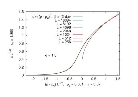
Figure 3: Data collapse plot of $s$ against $\rho$ for $\sigma=1.5$. The exponent $\nu$ is the same as in Fig. 2b, but $d_{f}$ and $\rho_{c}$ are slightly re-adjusted for best collapse. Also plotted is a power law $s=const\,(\rho-\rho_{c})^{\beta}$, showing that Eqs. (5) and (9) are well satisfied.

The critical threshold $\rho_{c}$ and the exponents $\nu$ and $\beta$ can also be estimated by using Eqs. (5) and (7). In Fig. 3 we show, again for $\sigma=1.5$, a data collapse plot in which we plotted $L^{2-d_{f}}s$ against $(\rho-\rho_{c})L^{1/\nu}$. We used the same value of $\nu$ as in Fig. 2b, but for optimal collapse we had to use slightly different values of $d_{f}$ and $\rho_{c}$. Since precise error estimates are difficult from such data collapse plots, we see these differences as rough error estimates. In addition, we show in Fig. 3 a curve indicating $const\,(\rho-\rho_{c})^{\beta}$, with $\beta=(2-d_{f})\nu$. It shows that Eqs. (5,9) are rather well satisfied.

Similar analyses were also made for other values of $\sigma$, but we do not report results since more precise estimates of critical parameters are obtained from gap scaling, as we shall show next.

IV.1.2 Gap scaling in the event-based ensemble

In the above conventional types of analyses, observables are studied at fixed values of the control parameters. It was suggested first by Manna and Chatterjee Manna (see also Refs. Nagler ; Fan ; Feshanjerdi ; Li2023 ) that more precise estimates could be obtained by studying observables at that value of the control parameter where the largest gap (i.e., the largest jump in the order parameter) occurs in individual realizations. These values fluctuate of course from realization to realization, and the ensemble of realizations at the point of maximal gap is called event-based ensemble in Ref. Li2023 . This was proposed for EP Manna ; Nagler , where these fluctuations are excessively large Christensen , and its usefulness for other percolation transitions was suggested in Refs. Fan ; Feshanjerdi .

That gap scaling studied at the points of maximal gaps is also useful in the present model is suggested by Fig. 4. There we plotted $P_{\rho}(\rho)$ (the distribution of maximal gap positions) at $L=2048$ and $\sigma=1.8$, and compared it to three curves of $\chi$ at the same value of $\sigma$ and for three different values of $L$. For easier comparison of their widths, we used the same arbitrary normalization for all four curves. It is clearly seen that $P_{\rho}(\rho)$ has the narrowest peak. It has the largest fluctuations, but this drawback is far outweighed by the sharpness of its peak.

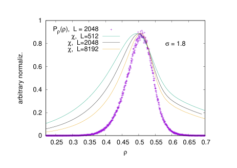
Figure 4: Plots of $P_{\rho}(\rho)$ (the distribution of maximal gap positions) and of the width $\chi$ of the order parameter distribution at given $\rho$ at $\sigma=1.8$. Normalization of all curves is such that they all have the same height, for easier comparison of their widths. It is seen that $P_{\rho}(\rho)$ has the sharpest peak, even if we compare it to curves of $\chi$ at different values of $L$.

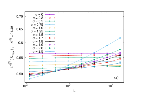
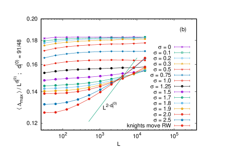
Figure 5: Log-log plots of $L^{-d_{f}^{(0)}}\langle S_{\rm max}\rangle$ (panel a) and of $L^{-d_{f}^{(0)}}\langle\Delta_{\rm max}\rangle$ (panel b) against $L$. In panel b we also show a straight line with the slope that would be expected for compact clusters ($d_{f}=2$).

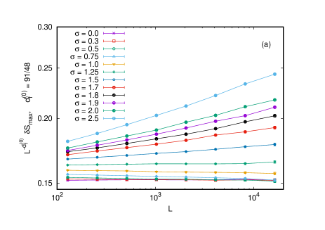
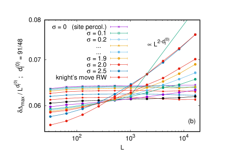
Figure 6: Log-log plots analogous to Fig. 5, but of $\delta S_{\rm max}=\{{\rm Var}[S_{\rm max}]\}^{1/2}$ (panel a) and $\delta\Delta_{\rm max}=\{{\rm Var}[\Delta_{\rm max}]\}^{1/2}$ (panel b), instead of $\langle S_{\rm max}\rangle$ and $\langle\Delta_{\rm max}\rangle$.

Fractal dimensions: Let us first look at the fractal dimensions. It can either be obtained from the average values and variances of $S_{\rm max}$ (the size of the giant cluster at criticality), or from the average values and variances of $\Delta_{\rm max}$ (which, as we pointed out, should scale like the size of the second-largest cluster). In Fig. 5 we show log-log plots of $L^{-d_{f}^{(0)}}\langle S_{\rm max}\rangle$ (panel a) and of $L^{-d_{f}^{(0)}}\langle\Delta_{\rm max}\rangle$ (panel b) against $L$, where $d_{f}^{(0)}=91/48$ is the fractal dimension in OP. We see in both panels that the curves are horizontal for $\sigma<1$, suggesting that the model is in the OP universality class for $\sigma<1$. For $\sigma>1$ there are, however, significant deviations which become more and more pronounced with increasing $\sigma$. But since all curves are strongly non-linear, it is impossible to quote with certainty an asymptotic power law for any $\sigma>1$. We also indicate in both panels the power laws $S_{\rm max}\sim\Delta_{\rm max}\sim L^{2}$, which we would expect for compact clusters. It is very strongly suggested that this is the asymptotic scaling for $\sigma>2$ (and for Knight’s move RWs), and we will later give strong arguments that there is no sharp percolation transition in this case. Whether there is a sharp transition for $\sigma=2$ is an open question.

Analogous plots for the (square roots of the) variances are shown in Fig. 6. Again both panels of Fig. 6 clearly show OP scaling for $\sigma<1$, and non-OP scaling for $\sigma>1$. But again it is impossible to determine the asymptotic scaling laws for $\sigma>1$, except that the data suggest strongly that clusters are compact for Levy flights with $\sigma>2$ and for the Knight’s move RWs.

All these results agree perfectly with what we obtained from the conventional analysis (data not shown). In particular, we understand now that the fractal dimensions used in Figs. 2b and 3 are only effective exponents valid in the studied range of $L$, and it should not surprise that they differ from each other.

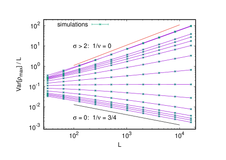
Figure 7: Plots of the variances of times of largest jumps as a function of $L$ for $\sigma=0.0,0.1,0.2,0.3,0.5,0.75,1.0,1.25,1.5,1.7,1.8,1.9,2,2.5$, and Knight’s move RW from the bottom to the top of the curves, respectively. The upper solid line corresponds to $\nu=\infty$ and seems to apply for $\sigma>2$ and Knight’s move RW, while the lower line corresponds to $\nu=4/3$ which holds for standard $2D$ percolation, and is consistent with our results within error bars for all $\sigma<0.5$.

Correlation length exponents: Correlation length exponents are obtained from the scalings of the shift of the averages of $\rho_{\rm max}$ and of the widths of their distributions. According to standard FSS, both give the same exponent $\nu$, but due to possible violations of the standard FSS scenario, this might not be the case in the present model.

Since measuring the shifts of $\bar{\chi}\equiv\langle\rho_{\rm max}\rangle$ with $L$ requires precise estimates of the true critical point positions, this is a somewhat delicate and error-prone procedure, in particular since we have already seen strong deviations from pure power law scalings. Thus we look first at the scaling of the variances. In Fig. 7 we show log-log plots of $L^{1/2}\chi_{\rho}$ against $L$, where

$$\chi_{\rho}=\{{\rm Var}[\rho_{\rm max}]\}^{1/2}\;.$$ (15)

We see now strong deviations from OP scaling for all $\sigma>0.5$. Superficially, all curves look rather straight so that $\nu$ seems well determined for each $\sigma>0.5$ and $1/\nu$ seems to increase continually with it, until $1/\nu=0$ for $\sigma>2$ (which would suggest that $\chi_{\rho}=const$ for $\sigma>2$). But more careful inspection shows that all curves for $\sigma<1$ bend downwards, while those for $\sigma>1$ bend up. Only the curve for $\sigma=1$ seems perfectly straight for $L>256$, with slope

$$\nu^{(\sigma=1)}=2.00\pm 0.03\;.$$ (16)

It is not clear what this means for the true asymptotic values of $\nu$. If the deviations from straight lines are a minor finite size correction (which is suggested superficially), then $1/\nu$ seems to decrease roughly linearly with $\sigma$ in the range $1/2<\sigma<2$, i.e.,

$$1/\nu=\left\{\begin{array}[]{r@{\quad:\quad}l}3/4&\sigma<1/2\\ 1-\sigma/2&1/2<\sigma<2\\ 0&\sigma>2\end{array}\right.$$ (17)

This would mean that the model is not in the OP class for $1/2<\sigma<1$, although we had clear evidence that $d_{f}$ there is the same as in OP.

Another, more radical, extrapolation could be the following: The curvatures seen in Fig. 7 imply that all curves for $\sigma<1$ align asymptotically with the one for $\sigma=0$, and those for $\sigma>1$ become finally parallel to that for $\sigma=2$. In this scenario, $\nu$ is would be constant for all $\sigma\neq 1$, and that it jumps at $\sigma=1$ from $4/3$ to $\infty$. Neither of these two scenarios is very plausible. A third one could be that $1/\nu=1/\nu^{(0)}$ for $\sigma<1$, and decreases then continuously to 0.

Whatever the correct scenario is, it is clear that $1/\nu=0$ for $\sigma>2$, which means that the order parameter curve $s$ versus $\rho$ becomes, for $\sigma>2$, independent of $L$, and in particular no singularity develops in the limit $L\to\infty$. Thus there is no percolation transition for $\sigma>2$.

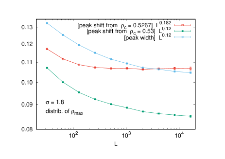
Figure 8: Log-log plots of $L^{1/\nu}\chi_{\rho}$ and of $(\bar{\rho}-\rho_{c})\,L^{1/\nu}$ versus $L$ for $\sigma=1.8$. For $\chi_{\rho}$ we choose $\nu$ such that the curve seems to become flat for large $L$. For $\bar{\rho}-\rho_{c}$ we show two curves: One, where the curve shows best scaling (for all $L>256$), the other with the same $\nu$ as for $\chi_{\rho}$ and with $\rho_{c}$ such that it becomes nearly a shifted copy of the one for $\chi_{\rho}$.

Let us now look at the values of $\bar{\rho}$ and their dependences on $\sigma$ and $L$. To be specific, take $\sigma=1.8$. In Fig. 7 we had seen that if there is a scaling law $\chi_{\rho}\sim L^{1/\nu}$, then there must be very large finite size corrections to it. In contrast, if we choose $\rho_{c}(\sigma=1.8)$ carefully, we can make the curve of $\log(\bar{\rho}-\rho_{c}(\sigma=1.8))$ versus $\log L$ nearly perfectly straight – but with a value of $\nu$ which is closer to $L^{1/\nu^{(0)}}$. This would support the conjecture that there are two different correlation length exponents. But there is also another, more plausible scenario: If we allow similarly large corrections to scaling for the dependence of $\bar{\rho}$ on $L$ as for $\chi_{\rho}$, we can find a value of $\rho_{c}$ such that the curves $\bar{\rho}-\rho_{c}$ versus $L$ and $\chi_{\rho}$ versus $L$ give practically the same value of $\nu$. This is demonstrated in Fig. 8, where we plotted both quantities against $L$ with suitably chosen values of $\nu$ and $\rho_{c}$. More precisely, in this log-log plot we show one curve for $\chi_{\rho}$ and two curves for $\bar{\rho}-\rho_{c}$ – one such that is it as straight as possible, the other such that it mimics $\chi_{\rho}$.

We thus conclude that the model definitely is not in the OP universality class for $\sigma>1$. The possible deviations from the conventional FSS picture due to a possible new length scale generated by the finite times of the Levy flights seem not to have led to two values of $\nu$, but they might be the source for the huge observed corrections to scaling.

IV.2 Three dimensions

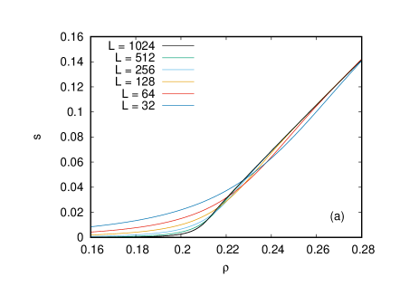
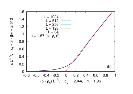
Figure 9: (a) Order parameter $s$ against $\rho$ for 3D generalized Knight’s move RW, for different lattice sizes $L$. Notice the region very near the critical point where curves cross each other (in contrast to OP and to the 2D Levy flight model discussed in the previous subsection).
(b) Data collapse plot of the data shown in panel a. The values of $\rho_{c}$ and of the exponents $\nu$ and $d_{f}$ are fitted to obtain best collapse. Also plotted is a power law $s=const\,(\rho-\rho_{c})^{\beta}$, showing that Eqs. (5) and (9) are well satisfied.

Here we just simulated the model with modified Knight’s move RWs. As said in the Introduction, the finiteness of the walk trajectory does not introduce an additional length scale in this case, whence we expect standard FSS.

Plots of the raw data of $s$ against $\rho$ for $L=64,128,256,512,$ 1024, and a collapse plot of these data analogous to Fig. 3 are shown in Fig. 9. In contrast to OP and all other percolation models we are aware of, the raw data curves cross each other, but the scaling relations Eqs. (5) and (9) are well satisfied. The exponent $\nu=1.96(2)$ is very different from that in OP, but the fractal dimension $d_{f}=2.512(10)$ is the same within errors. These values are still preliminary (we will say more about critical exponents when discussing $\chi$ and gap statistics), but we can already say now that these data do not seem to suffer from large corrections to scaling, in contrast to those of the previous subsection.

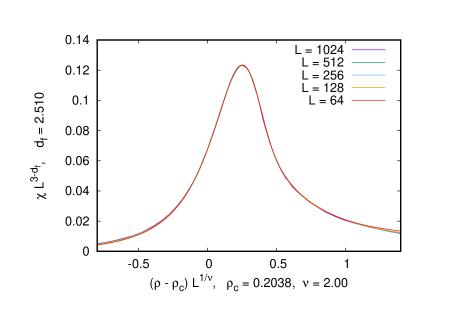
Figure 10: Data collapse plot of $\chi$ against $\rho$ for 3D generalized Knight’s move RWs. The numerical values of the critical parameters were, as in all previous collapse plots, obtained by eyeball fits.

A collapse plot of $\chi$ (analogous to Fig. 2) is shown in Fig 10. We see a very good data collapse, albeit for sightly different values of the critical parameters. These differences give a first impression of error estimates.

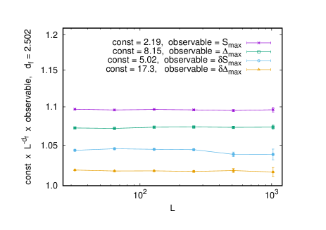
Figure 11: Log-log plots, for the modified Knight’s move RW in 3D, of the four event-based observables ($S_{\rm max},D_{\rm max}$, and the square roots of their variances) which should scale $\sim L^{d_{f}}$ at the critical point. For easier comparison, each curve is shifted vertically by an arbitrary factor and is divided by $L^{d_{f}}$. Please notice the very much blown-up y scale in this and in the following figure.

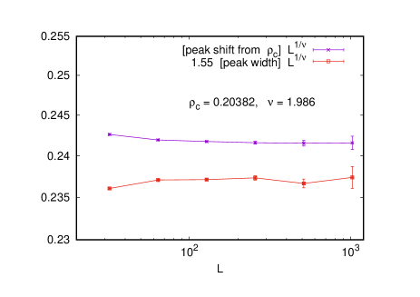
Figure 12: Log-log plots analogous to those in Fig. 8 of the $L$-dependence of the width of the peak of $\rho_{\max}$ and of its shift from $\rho_{c}$, but for the modified Knight’s move RW in 3D. In contrast to Fig. 8, we find now very good scaling, with the same value of $\nu$ for both curves. Notice again the very much blown-up y scale.

The fact that FSS is satisfied this time with small corrections, and that critical exponents can be determined rather precisely, is supported by looking at event-based gap scaling. In Fig. 11 we show the four observables which should scale with the fractal dimension ($S_{\rm max},D_{\rm max}$, and the square roots of their variances). For easier comparison, we multiply each by an arbitrary constant and divide it by $L^{d_{f}}$. The best fit is obtained with

$$d_{f}=2.502(5),$$ (18)

which represents our final estimate.

When determining the correlation exponent $\nu$, we are faced again with the fact that we have to know the precise value of the critical point $\rho_{c}$, if we want to check that the width of the critical peak and its shift from $\rho_{c}$ scale with the same power of $L$. But in contrast to the case of 2D Levy flights, there does not seem to be a problem now, as shown in Fig. 12. From this figure we obtain our best estimates

$$\rho_{c}=0.20382(5)\;,\;\;\;\nu=1.99(1).$$ (19)

It was conjectured in Refs. Weinrib-Halperin ; Weinrib that, for $3\leq d\leq 6$, one has $\nu=2/a$, if the correlation decays as $C(r)\sim r^{-a}$. According to Ref. Kantor , the sites visited by a RW and the sites not visited by it are correlated with $a=d-2$. Thus the present aftermath percolation model with (generalized) Knight’s move walks should be in the same universality class as pacman percolation in $3\leq d\leq 6$, and, in particular, for $d=3$ we expect $\nu=2$ in perfect agreement with our simulations Grass-pacman . In view of this agreement, we also conjecture that $d_{f}$ and $\beta$ are simple rationals, i.e.,

$$\nu=2,\;\;d_{f}=5/2,\;\;\beta=1.$$ (20)

This is also compatible with the estimates of Ref. Abete , who found $\nu=1.8(1)$ and $\beta=1.0(1)$ for pacman percolation, and is fully confirmed by somewhat less extensive simulations of aftermath percolation with NNN-RW’s, for which $\rho_{c}=0.2120(3)$.

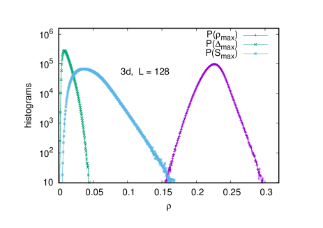
Figure 13: Histograms of $S_{\rm max},\rho_{\rm max}$, and $\Delta_{\rm max}$ for aftermath percolation with Knight’s move RW in d=3 for $L=128$, based on a sample of $4\,500\,000$ realizations.

In the present paper we also measured the distributions of $S_{\rm max},\rho_{\rm max}$, and $\Delta_{\rm max}$ and their scaling functions defined in Eqs.(11), (12), and (13). It was claimed in Ref. Fan that these are super-universal (i.e., universal across different universality classes) and the same even in discontinuous percolation transitions. Due to the possible difficulties with scaling violations mentioned above, we postpone their discussions for the model with Levy flights to a forthcoming paper, where we shall also discuss several other models. Here we present just one figure for the Knight’s move RW in three dimensions (Fig. 13). In this figure we show the three distributions for $L=128$. According to Ref. Fan , the distribution of $S_{\rm max}$ should be Gumbel and should thus have an exponential right-hand tail, while the two other distributions should fall off faster than exponential. The opposite is true: $P_{\rho}(\rho_{\rm max})$ and $P_{\Delta}(\Delta_{\rm max})$ seem to fall off exponentially, while $P_{S}(S_{\rm max})$ falls off faster. More details will be given in Ref. Fesh-distrib .

V Conclusions

In this paper, we have introduced a new version of CP. Motivated by the fact that disasters like wars, floods, or hurricanes often leave a weakened region which then falls easy prey to a second disaster like an epidemic, we have studied percolation restricted to the sites visited by generalized RWs. Essentially, this aftermath epidemic model is the inverse of pacman percolation Abete ; Kantor , where percolation is restricted to the sites not visited by a RW.

A crucial difference from pacman percolation is that the sites not visited by ordinary RWs are not connected, while those visited are. Thus, to obtain nontrivial percolation in aftermath epidemics, one has to use generalized walks where the visited sites are not connected. We studied Levy flights in two dimensions, and Knight’s move RWs both in two and three dimensions.

In three dimensions (and with Knight’s move RWs), we found that our model is in the same universality class as pacman percolation, and we conjecture that not only $\nu=2$ is a simple rational, but also $d_{f}=5/2$.

Knight’s move RWs in 2D do not lead to a sharp percolation transition. This is analogous to pacman percolation, where one also has to go to three or more dimensions to find a sharp transition. But for Levy flights, sharp transitions are found whose universality classes seem to depend on the Levy flight exponent $\sigma$.

As a control parameter, one can take in these models the number of walker steps or the number of visited points. Since finite walks might introduce new length scales, one has to worry that this breaks scale invariance and thereby violates one of the essential assumptions in the theory of critical phenomena. We find that this is indeed the case for Levy flights (but not for Knight’s move RWs). Thus, it is not obvious that the usual FFS applies. We found indeed no such problem for Knight’s move RWs in 3D. But we found problems in the form of very poor scaling in the case of Levy flights. It is not clear whether these are finite-size corrections, or whether they show that FSS is basically broken in this model. Another effect induced by additional length scales could be that different observables with the same scaling dimension show different critical exponents. In particular, we looked carefully into the possibility that there are two different correlation exponents, as has been found in some other nonstandard percolation models. We found no such deviation from FSS.

Figure 14: Correlation sum of visited sites by a Levy flight $\sigma=1.5$ with $T=0.96L^{2}$ steps on a square lattice of size $L=16384$, multiplied by $(L/r)^{2}$ and plotted over $r/L$. The density of visited points for this $T$ is roughly 0.55, i.e., the critical density at the percolation threshold. The curve is obtained by averaging over 2000 realizations, thus the deviations from a smooth curve are not due to noise but due to the discreteness of the lattice.

When simulating and analyzing these models, we used the fast NZ algorithm. This implied that we could very quickly determine quantities like cluster masses and gaps i.e., jumps in the leading cluster mass), but not spanning probabilities. Thus, we have not considered the latter, nor have we looked at backbones or conductivity exponents. But we have analyzed our data both within the traditional paradigm where one considers observables at given values of the control parameter, and in the event-based ensemble Manna ; Nagler ; Li2023 , where observables are measured at those control parameter values where the biggest gap occurs. We found that the latter gives, in general, more precise results.

VI Appendix

To measure correlations between sites visited by a Levy flight in two dimensions, we measured the correlation sum $C(r)$, i.e., the fraction of pairs of visited sites which are a distance $\leq r$ apart. This is shown in Fig. 14 for $\sigma=1.5$, $L=16384,$ and $T=0.96L^{2}$, which corresponds to a density $\rho=0.55$ of visited sites. For better resolution, we multiplied this by $(L/r)^{2}$, so the curve would be a horizontal flat line for a Poisson process, i.e., for $\sigma=0$. We see only very small deviations from this, and definitely no power law.

Acknowledgements: M.F. and A.A.M. acknowledge supports from the research council of the Alzahra University. P.G. thanks Nuno Araújo, Michael Grady, Hans Herrmann, and Yacov Kantor for discussions about CP.

References

- (1) M. Smallman-Raynor, and A. D. Cliff, War Epidemics: An Historical Geography of Infectious Diseases in Military Conflict and Civil Strife, 1850-2000, (Oxford University Press, 2004).
- (2) D. Stauffer, and A. Aharony, Introduction To Percolation Theory, (Taylor and Francis, 1991).
- (3) M. Sahimi, Applications of percolation theory, (CRC Press, 2003).
- (4) N.T.J. Bailey, The Mathematical Theory of Infectious Diseases, (Hafner Press, New York 1975).
- (5) W.D. Kermack, and A.G. McKendrick, A contribution to the mathematical theory of epidemics, J. Royal Stat. Soc. A115, 700 (1927); A138, 55 (1932).
- (6) P. Grassberger, On the critical behavior of the general epidemic process and dynamical percolation, Math. Biosci. 63, 157 (1983).
- (7) A.A. Saberi, Recent advances in percolation theory and its applications, Physics Reports 578, 1 (2015).
- (8) N. Araújo, P. Grassberger, B. Kahng, K.J. Schrenk, and R.M. Ziff, Recent advances and open challenges in percolation, The European Physical Journal Special Topics 223, 2307 (2014).
- (9) M.E. Newman, Networks (Oxford University Press, 2018).
- (10) H. Andersson, and T. Britton, Stochastic Epidemic Models and Their Statistical Analysis, (Springer, New York, 2000).
- (11) A. Barrat, M. Barthelemy, and A. Vespignani, Dynamical Processes on Complex Networks, (Cambridge University Press, Cambridge, 2008).
- (12) H. Hinrichsen, Non-equilibrium critical phenomena and phase transitions into absorbing states, Advances in Physics 49, 815 (2000).
- (13) T. Granger, T. M. Michelitsch, M. Bestehorn, A. P. Riascos, and B. A. Collet, Four compartment epidemic model with retarded transition rates, Phys. Rev. E 107, 044207 (2023).
- (14) J. Adler, Boostrap percolation, Physica A171, 453 (1991).
- (15) M.A. Di Muro, L.D. Valdez, H.E. Stanley, S.V. Buldyrev, and L.A. Braunstein, Insights into bootstrap percolation: Its equivalence with k-core percolation and the giant component, Phys. Rev. E 99, 022311 (2019).
- (16) H.-K. Janssen, M. Müller, and O. Stenull, Generalized epidemic process and tricritical dynamic percolation; Phys. Rev. E 70, 026114 (2004).
- (17) G. Bizhani, M. Paczuski, and P. Grassberger, Phys. Rev. E 86, 011128 (2012).
- (18) S.N. Dorogovtsev, A.V. Goltsev, and J.F.F. Mendes, K-core (bootstrap) percolation on complex networks: Critical phenomena and nonlocal effects, Phys. Rev. Lett. 96, 040601 (2006).
- (19) W. Cai, L. Chen, F. Ghanbarnejad, P. Grassberger, Avalanche outbreaks emerging in cooperative contagions, Nature Physics 11, 936 (2015).
- (20) P. Grassberger, “Spreading of epidemic processes leading to fractal structures,” in Fractals in Physics, edited by L. Pietronero and E. Tosatti, p. 273 (Elsevier, 1986).
- (21) F. Linder, J. Tran-Gia, S.R. Dahmen, and H. Hinrichsen, Long-range epidemic spreading with immunization, J. Phys. A 41, 185005 (2008).
- (22) P. Grassberger, SIR epidemics with long-range infection in one dimension, J. Stat. Mech. P04004 (2013).
- (23) P. Grassberger, Two-dimensional SIR epidemics with long range infection, J. Stat. Phys. 153, 289 (2913).
- (24) G. Gori, M. Michelangeli, N. Defenu, and A. Trombettoni, One-dimensional long-range percolation: a numerical study, Phys. Rev. E. 96, 012108 (2017).
- (25) V. Belik, T. Geisel, and D. Brockmann, Recurrent host mobility in spatial epidemics: beyond reaction-diffusion, Eur. Phys. J. B 84, 579 (2011)
- (26) V. Belik, T. Geisel, and D. Brockmann, Natural Human Mobility Patterns and Spatial Spread of Infectious Diseases, Phys. Rev. X 1, 011001 (2011).
- (27) D. Achlioptas, R.M. D’Souza, and J. Spencer, Explosive percolation in random networks, Science 323, 1453–1455 (2009).
- (28) P. Grassberger, C. Christensen, G. Bizhani, S.W. Son, and M. Paczuski, Explosive percolation is continuous, but with unusual finite size behavior, Phys. Rev. Lett. 106, 225701 (2011).
- (29) Ming Li, Junfeng Wang, Youjin Deng, Explosive Percolation Obeys Standard Finite-size Scaling in Event-based Ensemble, arXiv preprint arXiv:2301.09774, (2023).
- (30) G. Bianconi and S.N. Dorogovtsev, Multiple percolation transitions in a configuration model of network of networks, Phys. Rev. E 89, 062814 (2014).
- (31) A. Coniglio, and A. Fierro, Correlated Percolation, Encyclopedia of Complexity and Systems Science, pp 1-28 (2016).
- (32) C.M. Fortuin and P.W. Kasteleyn, On the random-cluster model: I. Introduction and relation to other models, Physica 57, 536 (1972).
- (33) M. Grady, Possible new phase transition in the 3D Ising Model associated with boundary percolation, arXiv preprint arXiv:2301.08424, (2023).
- (34) A. Weinrib and B. I. Halperin, Critical phenomena in systems with long-range-correlated quenched disorder, Phys. Rev. B. 27, 413 (1983).
- (35) A. Weinrib, Long-range correlated percolation, Phys. Rev. B. 29, 387 (1984).
- (36) K.J. Schrenk, N. Pose, J.J. Kranz, L.V.M. van Kessenich, N.A.M. Araújo, H.J. Herrmann, Percolation with long-range correlated disorder, Phys. Rev. E. 88, 052102 (2013).
- (37) T. Abete, A. de Candia, D. Lairez, and A. Coniglio, Percolation model for enzyme gel degradation, Phys. Rev. Lett. 93, 228301 (2004).
- (38) Y. Kantor and M. Kardar, Percolation of sites not removed by a random walker in d dimensions, Phys. Rev. E 100, 022125 (2019).
- (39) https://commons.wikimedia.org/wiki/File:Timur_Golden_Horde_campaign.jpg (accessed July 14, 2023).
- (40) https://www.heimatundwelt.de/kartenansicht.xtp?artId=978-3-14-100263-8&stichwort=Konfession&fs=1 (accessed July 14, 2023).
- (41) B.B. Mandelbrot, The Fractal Geometry of Nature, (W.H. Freeman, New York 1982).
- (42) M.E.J. Newman, and R.M. Ziff, Fast Monte Carlo algorithm for site or bond percolation, Phys. Rev. E 64, 016706 (2001).
- (43) J. Fan, J. Meng, Y. Liu, A.A. Saberi, J. Kuths, and J. Nagler, Universal gap scaling in percolation, Nature Physics 16, 455 (2020).
- (44) R.M. Ziff, Spanning probability in 2D percolation, Phys. Rev Lett. 69, 2670 (1992).
- (45) A. Margolina, H.J. Herrmann, and D. Stauffer, Size of largest and second largest cluster in random percolation, Phys. Lett. A93, 73 (1982).
- (46) S.S. Manna and A. Chatterjee, A new route to explosive percolation, Physica A390, 177 (2011).
- (47) J. Nagler, A. Levina, and M. Timme, Impact of single links in competitive percolation, Nature Physics 7, 265 (2011).
- (48) M. Feshanjerdi and A.A. Saberi, Universality class of epidemic percolation transitions driven by random walks, Phys. Rev. E 104, 064125 (2021).
- (49) M. Feshanjerdi and P. Grassberger, On Pacman and Aftermath Percolation, to be published (2023).
- (50) M. Feshanjerdi and P. Grassberger, Extreme-value statistics and super-universality in critical percolation?, to be published (2023).