A Distributionally Robust Random Utility Model

Abstract

This paper introduces the distributionally robust random utility model (DRO-RUM), which allows the preference shock (unobserved heterogeneity) distribution to be misspecified or unknown. We make three contributions using tools from the literature on robust optimization. First, by exploiting the notion of distributionally robust social surplus function, we show that the DRO-RUM endogenously generates a shock distribution that incorporates a correlation between the utilities of the different alternatives. Second, we show that the gradient of the distributionally robust social surplus yields the choice probability vector. This result generalizes the celebrated William-Daly-Zachary theorem to environments where the shock distribution is unknown. Third, we show how the DRO-RUM allows us to nonparametrically identify the mean utility vector associated with choice market data. This result extends the demand inversion approach to environments where the shock distribution is unknown or misspecified. We carry out several numerical experiments comparing the performance of the DRO-RUM with the traditional multinomial logit and probit models.

Keywords: Discrete choice, Random utility, Convex analysis, Distributionally robust optimization.

JEL classification: C35, C61, D90.

1 Introduction

The random utility model (RUM) introduced by Marschak (1959), Block and Marschak (1959), and Becker et al. (1963) has become the standard approach to model stochastic choice problems. The fundamental work of McFadden (1978a, c, 1981) makes the RUM an empirically tractable approach suitable for applications in many areas of applied microeconometric, including labor markets, industrial organization, health economics, transportation, and operations management. In particular, McFadden provides an economic foundation and econometric framework which connects observable to stochastic choice behavior. This latter feature makes the RUM suitable to deal with complex choice environments and welfare analysis (McFadden (2001) and Train (2009)).

In a RUM a decision maker (DM) faces a discrete choice set of alternatives in which each option is associated with a random utility. Then the DM chooses a particular option with a probability equal to the event that such alternative yields the highest utility among all available alternatives. Most of the applied literature models the random utility associated with each alternative as the sum of an observable and deterministic component and a random preference shock. Under this additive specification, different distributional assumptions on the random preference shock will generate different stochastic choice rules. Thus, all the effort is to provide conditions on the distribution of the preference shock such that the choice probabilities are consistent with the random utility maximization hypothesis (McFadden (1981)).

More importantly, assuming that the shock distribution is known to the analyst, we can estimate the parameters describing the deterministic utility associated with each alternative, carry out counterfactual welfare analysis, and predict future choice behavior. From a modeling standpoint, this assumption means that the analyst can correctly specify the shock distribution that describes the unobserved heterogeneity in DM’s behavior.

In this paper, we develop a RUM framework that allows for the possibility that the analyst (or the DM) does not know the true shock distribution. In doing so, we propose a distributional robust framework that relaxes the assumption that the shock distribution is known in advance. In particular, we develop a RUM framework that allows for misspecification in the shock distribution. By modeling the uncertainty regarding the true distribution, we follow the distributionally robust optimization literature and consider an environment where the analyst has access to a reference distribution $F$. This distribution corresponds to an approximation of the true statistical law generating the realizations of preference shocks. We refer to $F$ as the nominal distribution. Accordingly, we model uncertainty distribution in terms of an uncertainty set, which consists of all probability distributions that are close to $F$. We rely on the concept of statistical divergences to measure the distance between probability distributions. More precisely, we use the notion of $\phi$-divergences (Csiszar (1967); Liese and Vajda (1987)). Examples of $\phi$-divergences include the Kullback-Leibler, Renyi, and Cressie-Read distances, among many others. Thus, the uncertainty set contains the nominal $F$ and all feasible distributions within a certain radius as measured by the $\phi$-divergence.

Based on the uncertainty set, we introduce the robust social surplus function, corresponding to the maximum social surplus achievable over all feasible distributions. Like the traditional RUM, the robust social surplus is a convex function that contains all the relevant information to study and understand our distributionally robust RUM (DRO-RUM).

1.1 Contributions

We make three contributions. First, we show that the analysis of the DRO-RUM corresponds to the study of the properties of a strictly convex finite dimensional stochastic optimization program. This characterization directly implies that the endogenous robust distribution associated with the DRO-RUM introduces correlation between the preference shocks, even when the nominal $F$ may assume independence.

Second, we show that the gradient of the robust social surplus function yields the choice probability vector. The latter result is a nontrivial generalization of the celebrated Williams-Daly-Zachary (WDZ) theorem to environments where the true shock distribution is unknown. Furthermore, we show that the DRO-RUM preserves the convex structure of the traditional RUM. In particular, we derive a robust Fenchel duality framework that connects the robust social surplus and its convex conjugate.

In our third contribution, we characterize the empirical content of the DRO-RUM. Formally, we show that for an observed choice probability vector, there exists a unique mean utility vector that rationalizes the observed data in terms of a DRO-RUM. In particular, we show that the mean utility vector corresponds to the gradient of the convex conjugate of the robust social surplus function. The economic content of our result comes from the fact the DRO-RUM can rationalize observed behavior (a choice probability vector) in terms of a unique mean utility vector, which corresponds to the unique solution of a strictly convex stochastic programming problem.

To conclude our theoretical contributions, we carry out several numerical simulations discussing the properties of our framework. In particular, we compare the choice behavior of the DRO-RUM with the multinomial logit (MNL) and multinomial probit MNP models. We mainly focus on the impact of the so-called robustness parameter, which determines the size of the feasible set, impacting the choice probabilities and the surplus function.

1.2 Related literature

Our paper is related to several strands of literature. First, our paper relates to the literature on RUMs and convex analysis. The closest articles to ours are the works by Chiong et al. (2016), Galichon and Salanié (2021), and Fosgerau et al. (2021). Similar to us, these papers exploit the convex structure of the RUM to study the nonparametric identification of the mean utility vector when aggregate market data is available (observed choice probabilities). Our paper and results differ substantially from their work by allowing a more flexible framework regarding distributional assumptions.

Second, our paper relates to the semiparametric choice model (SCM) literature. The work by Natarajan et al. (2009) introduces the SCM in an environment where the true joint distribution is unknown, but the analyst has access to the set of marginal distributions associated with each alternative. This particular instance of the SCM is known as the marginal distribution model (MDM). Mishra et al. (2014) studies the MDM approach’s theoretical and empirical performance. Mishra et al. (2012) study a second instance of the SCM, which exploits cross moments constraints. In particular, they assume that the true distribution is unknown but the analyst has access to the true variance-covariance matrix that captures the correlation structure across the set of discrete alternatives.

At first glance, our approach is similar to SCM. As discussed by Feng et al. (2017), the latter are generally defined by a supremum over a set of distributions. We adapt to this definition by introducing the DRO-RUM, where the true distribution is unknown, and the analyst, therefore, considers all distributions in an uncertainty set.

Despite the similarity between the general SCM and our approach, both frameworks have important differences. First, our approach requires no assumption on the marginals or variance-covariance matrix. Instead, our model only requires knowledge of a nominal distribution. Second, using the concept of $\phi$-divergence enables the researcher to incorporate robustness, where she can control the uncertainty concerning the shock distribution by selecting the robustness parameter. Hence, the feasible set is not determined explicitly by fixing some moments or marginal distributions but is rather implicitly constructed by choosing the nominal distribution and the magnitude of the robustness parameter. Moreover, our approach can generate different models by allowing the choice of several $\phi$-divergence functions and different nominal distributions. Third, we show that the DRO-RUM preserves the convex structure (and duality) of the traditional RUM approach. In particular, we generalize the WDZ and provide a robust Fenchel duality analysis. Fourth, we identify the mean utility vector nonparametrically by exploiting our robust convex duality results. This result allows us to rationalize aggregate market data (choice probabilities) in terms of a DRO-RUM. In particular, our identification result corresponds to a robust demand inversion method. Our paper is also related to the literature on robustness in macroeconomics (Hansen and Sargent (2001, 2008)). However, this literature focuses on recursive problems using the Kullback-Leibler distance. The recent paper by Christensen and Connault (2023) introduces robustness ideas to analyze the sensitivity of counterfactuals to parametric assumptions about the distribution of latent variables in structural models. Their focus is different from the problem we study in this paper. Finally, our paper is closely related to the literature on distributionally robust optimization. Shapiro (2017a) and Kuhn et al. (2019) provide an up-to-date treatment of the subject. Applications vary from inventory management to regularization in machine learning.However, to our knowledge, this literature has not studied the problem of the distributional robustness of the RUM.

The rest of the paper is organized as follows. Section 2 reviews the traditional RUM approach and introduces the problem of robustness. Section 3 presents the DRO-RUM model and discusses its main properties. The empirical content of the DRO-RUM approach is discussed in Section 4. Section 5 contents several numerical experiments comparing the outcome of the DRO-RUM with respect to MNL and MNP. Section 6 concludes the paper by providing an overview of possible extensions.

Notation. Throughout the paper we use the following notation and definitions. Let us denote $\bar{\mathbb{R}}=\mathbb{R}\cup\left\{-\infty,+\infty\right\}$ and consider extended real-valued functions

$$f:\mathbb{V}\to\bar{\mathbb{R}},$$

where $\mathbb{V}$ is a finite dimensional real vector space. Consequently, we denote by $\mathbb{V}^{*}$ its dual space consisting of all linear functionals. In particular, we often work with subspaces of $\mathbb{R}^{n}$. The set defined by

$$\mbox{dom}f=\left\{x\in\mathbb{V}:f(x)<+\infty\right\}$$

is called the (effective) domain of $f$. A function is said to be proper if it takes nowhere the value $-\infty$ and $\mbox{dom}f\neq\emptyset$. For a proper function $f:\mathbb{V}\to\bar{\mathbb{R}}$ the set $\partial f(x)$ represents its subdifferential at $x\in\mbox{dom}f$, i.e.

$$\partial f(x)=\left\{g\in\mathbb{V}^{*}:f(y)\geq f(x)+\langle g,y-x\rangle,\quad\mbox{for all}\quad y\in\mathbb{R}^{n}\right\},$$

where $g\in\mathbb{V}^{*}$ is said to be a subgradient. If the subdifferential set is a singleton, i. e. the subgradient $g$ is unique, we denote by $\nabla f(x)$ the gradient of the function $f$ at $x\in\mbox{int}\left(\mbox{dom}f\right)$. The convex conjugate of a proper function $f:\mathbb{V}\to\bar{\mathbb{R}}$ is

$$f^{*}(g)=\underset{x\in\mathbb{V}}{\sup}\left\{\left\langle x,g\right\rangle-f(x)\right\},\quad g\in\mathbb{V}^{*}.$$

$\mathbb{E}_{F}(\cdot)$ denotes the expectation operator with respect to a distribution $F$.

2 The Random Utility Model

Consider a decision maker (DM) making a utility-maximizing discrete choice among alternatives $j\in\mathcal{J}=\left\{0,1,\ldots,J\right\}$. The utility of option $j$ is

$$\tilde{u}_{j}=u_{j}+\varepsilon_{j},$$ (1)

where $u=(u_{0},u_{1},\ldots,u_{J})^{T}$ is deterministic and $\varepsilon=(\varepsilon_{0},\varepsilon_{1},\ldots,\varepsilon_{J})^{T}$ is a vector of random utility shocks. The alternative $0$ has the interpretation of an outside option. Following the discrete choice literature, we set $u_{0}=0$.

Following McFadden (1978a, 1981), the previous description corresponds to the classic additive random utility model (RUM). Our presentation of the RUM framework here will emphasize convex-analytic properties.

Assumption 1

The random vector $\varepsilon$ follows a distribution $F$ that is absolutely continuous with finite means, independent of $u$, and fully supported on $\mathbb{R}^{J+1}$.

Assumption 1 leaves the distribution of $\varepsilon$ unspecified, thus allowing for a wide range of choice probability systems far beyond the often-used logit model. The assumption allows arbitrary correlation between the $\varepsilon_{j}$’s may be important in applications. As a direct consequence of Assumption 1, the DM’s choice probabilities correspond to:

$$p_{j}(u)\equiv\mathbb{P}\left(u_{j}+\varepsilon_{j}=\max_{j^{\prime}\in\mathcal{J}}\left\{u_{j^{\prime}}+\varepsilon_{j^{\prime}}\right\}\right),\quad j=0,1,\ldots,J.$$

An important object in the RUM framework is the surplus function of the discrete choice model (so named by McFadden (1981)). It is given by

$$W\left(u\right)=\mathbb{E}_{F}\left[\max_{j\in\mathcal{J}}\left\{u_{j}+\varepsilon_{j}\right\}\right].$$ (2)

Under Assumption 1, $W$ is convex and differentiable and the choice probability vector $p(u)$ coincides with the gradient of $W$:

$$\frac{\partial}{\partial u_{k}}W\left(u\right)=p_{k}(u)\,\,\,\mbox{for $k=0,1,\ldots,J$}$$

or, using vector notation, $p\left(u\right)=\nabla W(u)$. The previous result is the celebrated Williams-Daly-Zachary (henceforth, WDZ) theorem, famous in the discrete choice literature (McFadden (1978a, 1981)).

One of the most widely used RUMs is the multinomial logit (MNL) model, which assumes that the entries of $\left(\varepsilon_{0},\varepsilon_{1},\ldots,\varepsilon_{J}\right)^{T}$ follow iid Gumbel distributions with scale parameter $\eta$. Given this assumption, we can write the social surplus function in closed form:

$$W(u)=\eta\log\left(\sum_{j=0}^{J}e^{u_{j}/\eta}\right)+\eta\gamma,$$ (3)

where $\gamma$ is the Euler-Mascheroni constant. It follows from (3) that the WDZ theorem implies that $p_{j}(u)$ is given by:

$$\frac{\partial W\left(u\right)}{\partial u_{j}}={e^{u_{j}/\eta}\over\sum_{l=0}^{J}e^{u_{l}/\eta}}\quad\mbox{for $j\in\mathcal{J}.$}$$ (4)

The MNL model belongs to a broader class of RUM models called generalized extreme value (GEV) models introduced by McFadden (1978b). This class of models is defined via a generating function $G:\mathbb{R}^{J+1}_{+}\rightarrow\mathbb{R}_{+}$, which has to satisfy the following properties:

• $G$ is homogeneous of degree $\frac{1}{\eta}>0$.

• $G\left(x_{0},x_{1},\ldots,x_{j},\ldots,x_{J}\right)\rightarrow\infty$ as $x_{j}\rightarrow\infty$, $j=0,1,\ldots,J$.

• For the partial derivatives of $G$ w.r.t. $k$ distinct variables it holds:

  $$\frac{\partial^{k+1}G\left(x_{0},\ldots,x_{J}\right)}{\partial x_{j_{0}},\partial x_{j_{1}}\cdots\partial x_{j_{k}}}\geq 0\mbox{ if }{k+1}\mbox{ is odd},\quad\frac{\partial^{k+1}G\left(x_{0},\ldots,x_{J}\right)}{\partial x_{j_{0}},\partial x_{j_{1}}\cdots\partial x_{j_{k}}}\leq 0\mbox{ if }{k+1}\mbox{ is even}.$$

McFadden (1978b, 1981) show that a function $G$ satisfying conditions (G1)-(G3) implies that the joint distribution of the random vector $\varepsilon$ corresponds to the following probability density function:

$$f_{\epsilon}\left(y_{0},y_{1},\ldots,y_{J}\right)=\frac{\partial^{J+1}\exp\left(-G\left(e^{-y_{0}},\ldots,e^{-y_{J}}\right)\right)}{\partial y_{0}\cdots\partial y_{J}},$$

An essential property of the GEV class is that the social surplus function corresponds to (McFadden, 1978b)

$$W(u)=\eta\ln G\left(e^{u}\right)+\eta\gamma,$$

where $\gamma$ is the Euler-Mascheroni constant. From the WDZ theorem it follows that the choice probability of the $j$-th alternative corresponds to:

$$p_{j}(u)=\frac{\partial W(u)}{\partial u_{j}}=\eta\frac{\partial G\left(e^{u}\right)}{\partial e^{u_{j}}}\cdot\frac{e^{u_{j}}}{G\left(e^{u}\right)}\quad\forall j\in\mathcal{J}.$$

It is easy to see that the generating function

$$G(e^{u})=\sum_{j=0}^{J}e^{u_{j}/\eta}=1+\sum_{j=1}^{J}e^{u_{j}/\eta}$$

leads to the MNL model.

The main advantage of the GEV class is its flexibility to capture complex patterns correlation across the random variables $\varepsilon_{j}$’s. Examples of this are the Nested Logit (NL), the Paired Combinatorial Logit (PCL), the Ordered GEV (OGEV), and the Generalized Nested Logit (GNL) model, which are particular instances of the GEV family.

2.1 A robust framework for the RUM

A fundamental assumption in the RUM is that the shock distribution is known to the researcher (and the DM). This means that the distribution of $\varepsilon$ is correctly specified. Our main goal in this paper is to relax this condition by allowing the distribution of $\varepsilon$ to be unknown. Instead, the distribution of $\varepsilon$ is an argument in an optimization problem that corresponds to the definition of the social surplus function. We formalize this idea by replacing expression (2) with the robust social surplus function:

$$W^{RO}(u)=\sup_{G\in\mathcal{M}(F)}\mathbb{E}_{G}\left[\max_{j\in\mathcal{J}}\left\{u_{j}+\varepsilon_{j}\right\}\right],$$ (5)

where $\mathcal{M}(F)$ is a set of probability distributions that are close to a predetermined distribution $F$ which satisfies Assumption 1. This distribution $F$ can be seen as a best guess or prior knowledge of the analyst regarding the joint distribution of error terms. We will refer to $F$ as nominal distribution. In order to be more robust against misspecification the analyst takes into account all possible distributions that are close to the nominal distribution. A key aspect of our approach is related to the structure of the set $\mathcal{M}(F)$. In Section 3 we specify the $\mathcal{M}(F)$ in terms of $\phi$-divergence functions, which enables us to use the notion of statistical divergences between probability distributions (Csiszar (1967), Liese and Vajda (1987), and Pardo (2005)). Hence, we will refer to this as the distributionally robust-RUM (DRO-RUM). As we shall see, by doing this we are able to characterize the resulting DRO-RUM surplus function in terms of a convex finite dimensional optimization program. This characterization is key in studying the properties of the DRO-RUM approach.

Let $G^{\star}$ denote the distribution (or a limit of a sequence of distributions) that attains the optimal value in (5). The choice probability for alternative $j$ under this model is given by (provided that it is well defined):

$$p_{j}^{RO}(u)=\mathbb{P}_{G^{\star}}\left(j=\arg\max_{j^{\prime}\in\mathcal{J}}\{u_{j^{\prime}}+\varepsilon_{j^{\prime}}\}\right)$$ (6)

From an economic standpoint, we can interpret the program (5) in two alternative ways. First, the robust-RUM considers a situation where a DM faces preference shocks but has some flexibility concerning the distribution generating those errors.
Second, an analyst might not be sure about the distribution of the random vector $\varepsilon$ but might consider a set of possible distributions instead. Thus, it is reasonable for the analyst to assume that the DM is rational and the shock distribution generating the social surplus corresponds to one of the elements in $\mathcal{M}$.

2.2 Connection with the semiparametric choice model

It is worth pointing out that the definition of the RO-RUM is similar to the semiparametric choice model (SCM), which has been recently introduced in the operation research literature (Natarajan et al. (2009)). The surplus functions are defined as the supremum over distributions in both model classes. By doing so, the SCM can capture complex substitution patterns and correlation between the different alternatives in the choice set $\mathcal{J}$. Feng et al. (2017) provide a detailed overview of several discrete choice models, where the authors refer to SCM as a supremum over a general set of distributions. Thus, the robust-RUM could be seen as an instance of a semi-parametric choice model. There are some existing instances of SCM in the literature. In their original paper, Natarajan et al. (2009) restrict the feasible set to joint distributions with given information on the marginal distributions. This particular instance of the SCM is known as the marginal distribution model (MDM). A second class of SCMs exploits cross-moment constraints. In particular, Mishra et al. (2012) study the cross-moment model (CMM), which considers the set $\mathcal{M}$ to be the set of distributions consistent with a known variance-covariance matrix.

Despite the apparent similarity, our approach differs from the existing SCM in several aspects. As we shall see in the rest of the paper, our framework differs from the SCM in the specification of the set of distributions. In particular, in existing SCMs the analyst needs to construct a feasible set explicitly, for instance, by fixing the marginal distributions. In contrast, in our robust approach, the analyst specifies the feasible set implicitly by determining the nominal distribution $F$ and by upper bounding the distance of other distributions to $F$. Hence, the DRO-RUM approach does not require knowledge of the marginals of either variance-covariance matrix. In Section 3, we see that in the DRO-RUM, the researcher controls the distance by selecting the magnitude of a robustness parameter. Thus, our approach follows a rather different principle than existing SCMs.

Additionally, we show that the DRO-RUM corresponds to the solution of a convex finite dimensional optimization problem. This latter fact allows us to extend the WDZ theorem to environments where the shock distribution is misspecified. Finally, Section 4 shows how the DRO-RUM enables us to recover the mean utility vector $u$.

3 A Distributionally Robust - RUM model

In this section, we formally introduce the DRO-RUM approach. Following the distributionally robust optimization literature, we consider an environment where the researcher (or the DM) has access to a reference distribution $F$, which may be an approximation (or estimate) of the true statistical law governing the realizations of $\varepsilon$. We refer to $F$ as the nominal distribution. Then, we define a set of probability distributions that are close to $F$. We rely on statistical distances to formalize the notion of distance between probability distributions.

3.1 $\phi$-divergences

We measure the distance between two probability distributions by the so-called $\phi$-divergence.
Let $\phi:\mathbb{R}\rightarrow(-\infty,+\infty]$ be a proper closed convex function such that $\mbox{dom}\;\phi$ is an interval with endpoints $\alpha<\beta$, so, $\operatorname{int}\left(\mbox{dom}\;\phi\right)=(\alpha,\beta)$. Since $\phi$ is closed, we have $\lim_{t\rightarrow\alpha_{+}}\phi(t)=\phi(\alpha)$, if $\alpha$ is finite and $\lim_{t\rightarrow\beta_{-}}\phi(t)=\phi(\beta)$, if $\beta$ is finite.

Throughout the paper we assume that $\phi$ is nonnegative and attains its minimum at the point $1\in\operatorname{int}\left(\mbox{dom}\;\phi\right)$, i.e. $\phi(1)=0$. The class of such functions is denoted by $\Phi$.

Definition 1

Given $\phi\in\Phi$, the $\phi$-divergence of the probability measure $G$ with respect to $F$ is

$$D_{\phi}(G\|F)=\left\{\begin{array}[]{cl}\int_{\mathbb{R}^{J+1}}\phi\left(\frac{g(\varepsilon)}{f(\varepsilon)}\right)f(\varepsilon)d\varepsilon&\text{ if }\mathrm{G}\ll\mathrm{F}\\ +\infty&\text{ otherwise }\end{array}\right.$$ (7)

where $f$ and $g$ are the associated densities of $F$ and $G$ respectively.

To avoid pathological cases, throughout the paper, we assume the following:

$$\phi(0)<\infty,0\cdot\phi\left(\frac{0}{0}\right)\equiv 0,0\cdot\phi\left(\frac{s}{0}\right)=\lim_{\varepsilon\rightarrow 0}\varepsilon\cdot\phi\left(\frac{s}{\varepsilon}\right)=s\lim_{t\rightarrow\infty}\frac{\phi(t)}{t},\quad s>0.$$ (8)

If the measure $G$ is absolutely continuous w.r.t. $F$, i. e. $G\ll F$, the $\phi$-divergence can be conveniently written as:

$$D_{\phi}(G\|F)=\mathbb{E}_{F}\left(\phi(L(\varepsilon))\right),$$ (9)

where $L(\varepsilon)\triangleq g(\varepsilon)/f(\varepsilon)$ is the likelihood ratio between the densities $g$ and $f$, also known as Radon-Nikodym derivative of the two measures. Using the expression (9) combined with the convexity of $\phi$, Jensen’s inequality implies that

$$D_{\phi}(G\|F)\geq\phi\left(\mathbb{E}_{F}\left(L(\varepsilon)\right)\right)=\phi(1)=0$$ (10)

with equality if $G=F$, so that $D_{\phi}(G\|F)$ is a measure of distance of $G$ from $F$. Furthermore, the $\phi$-divergence functional is convex in both of its arguments. The following proposition summarizes these key properties.

Proposition 1

The $\phi$-divergence functional (7) is well-defined and nonnegative. It is equal to zero if and only if $f_{1}(t)=f_{2}(t)$ a.e. Furthermore, $D_{\phi}$ is convex on each of its arguments.

Proof. The proof that $D_{\phi}(G\|F)$ is well defined and nonnegative follows from (Ben-Tal and Teboulle, 1987, Prop. 1). The convexity of $D_{\phi}$ follows from (Ben-Tal and Teboulle, 1987, Prop. 2).  $\square$

In our analysis, a key element will be the convex conjugate of $\phi$. For $\phi\in\Phi$ its conjugate denoted by $\phi^{*}$ is:

$$\phi^{*}(s)=\sup_{t\in\mathbb{R}}\{st-\phi(t)\}=\sup_{t\in\operatorname{dom}\phi}\{st-\phi(t)\}=\sup_{t\in\operatorname{int}\operatorname{dom}\phi}\{st-\phi(t)\},$$ (11)

where the last equality follows from (Rockafellar, 1970, Cor. 12.2.2). The conjugate $\phi^{*}$ is a closed proper convex function, with int dom $\phi^{*}=(a,b)$, where

$$a=\lim_{t\rightarrow-\infty}t^{-1}\phi(t)\in[-\infty,+\infty);b=\lim_{t\rightarrow+\infty}t^{-1}\phi(t)\in(-\infty,+\infty].$$

Moreover, since $\phi$ is convex and closed, we have for its bi-conjugate $\phi^{**}=\phi$, (Rockafellar (1970)). It is worth noting that using the fact that $1$ is the minimizer of $\phi$ and it is in the interior of its domain, so $\phi^{\prime}(1)=0$ holds. In addition, using the property that $\phi$ is convex and closed, we have by Fenchel equality $y=\phi^{\prime}(x)$ iff $x=\phi^{*^{\prime}}(y)$. Applying this latter observation to $x=1$ and $y=0$ we obtain $\phi^{\ast\prime}(0)=1$.

3.2 The DRO-RUM framework

The main idea is to consider an environment where the analyst (or a DM) does not know the true distribution governing realizations of the shock vector $\varepsilon$. In this environment, the role of $F$ is an approximation or some best guess of the “true” unknown distribution. Recognizing this ambiguity or potential misspecification of the distribution $F$, we make use of the $\phi$-divergence to define the uncertainty set $\mathcal{M}_{\phi}(F)$ as:

$$\mathcal{M}_{\phi}(F)=\{G\ll F:D_{\phi}(G||F)\leq\rho\},$$ (12)

Formally, $\mathcal{M}_{\phi}(F)$ is the set of all probability measures $G$ that are absolutely continuous w.r.t $F$, whose distance from $F$, as measured by the $\phi$-divergence, is at most $\rho$. The hyperparameter $\rho$ is the radius of $\mathcal{M}_{\phi}(F)$, which reflects how uncertain is the researcher (or the DM) about the plausibility of $F$ being correct. Let us further elaborate on this interpretation. Following Hansen and Sargent (2001, 2008), Shapiro (2017b), and Kuhn et al. (2019), we interpret the set (12) as an environment in which the analyst (or the DM) has some best guess $F$ of the true unknown probability distribution, but does not fully trust it. For instance, the researcher may consider that the nominal distribution $F$ corresponds to the Gumbel distribution. In this case, $\mathcal{M}_{\phi}(F)$ accounts for many other probability distributions $G$ to be feasible, where $\rho$ determines the size of the feasible set.

Endowed with the set $\mathcal{M}_{\phi}(F)$, we can modify expression (5) to obtain a distributionally robust surplus function. Thus, the surplus function of the DRO-RUM corresponds to the following optimization problem:

$$W^{DRO}(u)=\sup_{G\in\mathcal{M}_{\phi}(\mathcal{F})}\left\{\mathbb{E}_{G}\left[\max_{j\in\mathcal{J}}\left\{u_{j}+\varepsilon_{j}\right\}\right]\right\}$$ (13)

Some remarks are in order. First, a fundamental aspect of program (13) is the role of the parameter $\rho$ which controls the size of $\mathcal{M}_{\phi}(F)$. Because of this, we can interpret $\rho$ as an index of robustness. More precisely, when $\rho=0$ we get $\mathcal{M}_{\phi}(F)=\{F\}$, which means that we recover the RUM under the distribution $F$. On the other hand, when $\rho\longrightarrow\infty$ the uncertainty set $\mathcal{M}_{\phi}(F)$ admits a much larger set of possible distributions, including those that may not satisfy Assumption 1. The DRO-RUM aims to set $\rho$ to reflect the perceived uncertainty that the researcher (or a DM) experiences about the distributional assumption for $\varepsilon$.

The following lemma establishes some elementary properties of $W^{DRO}(u)$.

Lemma 1

For the DRO-RUM the surplus function $W^{DRO}(u)$ satisfies:

• $W^{DRO}(u+c\cdot e)=W^{DRO}(u)+c$ for all $c\in\mathbb{R},u\in\mathbb{R}^{J}$.

• $W^{DRO}(u)\geq W^{DRO}(v)$ for all $u,v\in\mathbb{R}^{J}$ with $u\geq v$.

• $W^{DRO}(u)\geq\displaystyle\max_{j\in\mathcal{J}}u_{i}+\min_{j\in\mathcal{J}}\mathbb{E}_{F}\left[\varepsilon_{i}\right]$.

• $W^{DRO}(u)$ is convex in $u$.

Proof.

• The definition provides

  $$W^{DRO}(u+c\cdot e)=\sup_{G\in\mathcal{M}_{\phi}(F)}\left\{\mathbb{E}_{G}\left[\max_{j\in\mathcal{J}}\left\{u_{j}+\varepsilon_{j}+c\right\}\right]\right\}$$

  Due to the linearity of the expectation, it holds

  $$c+\sup_{G\in\mathcal{M}_{\phi}(F)}\mathbb{E}_{G}\left[\max_{j\in\mathcal{J}}\left\{u_{j}+\varepsilon_{j}\right\}\right]=c+W^{DRO}(u).$$

• Take any $u,v\in\mathbb{R}^{J}$ with $u\geq v$. First we note that for any arbitrary feasible distribution $G\in\mathcal{M}_{\phi}(F)$ it holds

  $$W^{DRO}(u)\geq\mathbb{E}_{G}\left[\max_{j\in\mathcal{J}}\left\{u_{j}+\varepsilon_{j}\right\}\right]\overset{(*)}{\geq}\mathbb{E}_{G}\left[\max_{j\in\mathcal{J}}\left\{v_{j}+\varepsilon_{j}\right\}\right],$$

  where $(*)$ holds due to the monotonicity of the expectation. Taking the supremum on the right-hand side, we conclude that $W^{DRO}(u)\geq W^{DRO}(v)$.

• We deduce that for any $i\in\mathcal{J}$

  $$W^{DRO}(u)\geq\mathbb{E}_{F}\left[\max_{j\in\mathcal{J}}\left\{u_{j}+\varepsilon_{j}\right\}\right]\geq\mathbb{E}_{F}\left[u_{i}+\varepsilon_{i}\right]\geq u_{i}+\min_{j\in\mathcal{J}}\mathbb{E}_{F}\left[\varepsilon_{j}\right],$$

  which is finite due to Assumption 1.

• Let $\alpha\in[0,1]$ and let $u$ and $v$ two deterministic utility vectors. For a fix distribution $G\in\mathcal{M}_{\phi}(F)$, Then, due to the convexity of the $\max\{\cdot\}$ operator,

  $$W^{DRO}(\alpha u+(1-\alpha)v)\leq\alpha\mathbb{E}_{G}\left(\max_{j\in\mathcal{J}}\{u_{j}+\varepsilon_{j}\}\right)+(1-\alpha)\mathbb{E}_{G}\left(\max_{j\in\mathcal{J}}\{v_{j}+\varepsilon_{j}\}\right).$$

  In the right-hand side, taking the supremum with respect to $G$ over $\mathcal{M}_{\phi}(F)$, we get

  $$W^{DRO}(\alpha u+(1-\alpha)v)\leq\alpha W^{DRO}(u)+(1-\alpha)W^{DRO}(v).$$

  Then the convexity of $W^{DRO}(u)$ follows.

The following result characterizes $W^{DRO}(u)$.

Proposition 2

Let Assumption 1 hold and define the random variable $H(u,\varepsilon)\triangleq\max_{j\in\mathcal{J}}\{u_{j}+\varepsilon_{j}\}$. Then, problem (13) is equivalent to solving the following finite-dimensional convex program:

$$W^{DRO}(u)=\inf_{\lambda\geq 0,\mu\in\mathbb{R}}\left\{\lambda\rho+\mu+\lambda\mathbb{E}_{F}\left[\phi^{*}\left({H(u,\varepsilon)-\mu\over\lambda}\right)\right]\right\},$$ (14)

where $\lambda$ is the Lagrange multiplier associated to the uncertainty set $\mathcal{M}_{\phi}(F)$ and $\mu$ the multiplier associated to $G$ being a probabality measure. Furthermore, the program (14) is convex in $\mu$ and $\lambda$.

Proof. This result follows from a direct application of (Ruszczyński and Shapiro, 2021, Prop. 7.9). For completeness, we provide the details of the argument. First, we note that for a fixed utility vector $u$ and using the likelihood ratio $L(\varepsilon)\triangleq dG(\varepsilon)/dF(\varepsilon)$, the DRO-RUM in (13) can be expressed as:

$$W^{DRO}(u) = \sup_{G}\{\mathbb{E}_{G}(H(u,\varepsilon)):G\in\mathcal{M}_{\phi}(F)\}$$ (15)

$$= \sup_{L\geq 0}\left\{\mathbb{E}_{F}[L(\varepsilon)H(u;\varepsilon)]\mid\mathbb{E}_{F}[\phi(L(\varepsilon))]\leq\rho,\mathbb{E}_{F}[L(\varepsilon)]=1\right\}$$

where the supremum is over a set of measurable functions.

The Lagrangian of problem (15) is :

$$\mathcal{L}(L,\lambda,\mu)=\int_{\mathbb{R}^{J+1}}[L(\varepsilon)H(u,\varepsilon)-\lambda\phi(L(\varepsilon))-\mu L(\varepsilon)]dF(\varepsilon)+\lambda\rho+\mu.$$ (16)

The Lagrangian dual of problem (16) is the problem

$$\inf_{\lambda\geq 0,\mu\in\mathbb{R}}\sup_{L\geq 0}\mathcal{L}(L,\lambda,\mu)$$ (17)

Since Slater condition holds for problem (16), there is no duality gap between (16) and its dual problem (17). Moreover, the dual problem has a nonempty and bounded set of optimal solutions.

By the interchangeability principle ((Rockafellar, 1976, Thm. 3A)), the maximum in (17) can be taken inside the integral, that is

$$\begin{gathered}\sup_{L\geq 0}\int_{\mathbb{R}^{J+1}}[L(\varepsilon)H(u,\varepsilon)-\mu L(\varepsilon)-\lambda\phi(L(\varepsilon))]dF(\varepsilon)\\ =\int_{\mathbb{R}^{J+1}}{\sup_{t\geq 0}\{t(H(u,\varepsilon)-\mu)-\lambda\phi(t)\}}dF(\varepsilon),\end{gathered}$$

Noting that $(\lambda\phi)^{*}(H(u,\varepsilon)-\mu)=\sup_{t\geq 0}\{t(H(u,\varepsilon)-\mu)-\lambda\phi(t)\}$, then it follows that

$$W^{DRO}(u)=\inf_{\lambda\geq 0,\mu\in\mathbb{R}}\left\{\lambda\rho+\mu+\mathbb{E}_{F}\left[(\lambda\phi)^{*}(H(u,\varepsilon)-\mu)\right]\right\}.$$ (18)

To show the convexity with respect to $\lambda$ and $\mu$ we note that it suffices in (17) and (18) to take the $\inf$ with respect to $\lambda>0$ rather than $\lambda\geq 0$, and that $(\lambda\phi)^{*}(y)=\lambda\phi^{*}(y/\lambda)$ for $\lambda>0$. Therefore $W^{DRO}(u)$ is given by the optimal value of the following problem:

$$\inf_{\lambda>0,\mu\in\mathbb{R}}\left\{\lambda\rho+\mu+\lambda\mathbb{E}_{F}\left[\phi^{*}((H(u,\varepsilon)-\mu)/\lambda)\right]\right\}$$ (19)

Note that $\phi^{*}(\cdot)$ is convex. Hence, $\lambda\phi^{*}(y/\lambda)$ is jointly convex in $y$ and $\lambda>0$. It follows that the objective function of problem (19) is a convex function of $\lambda>0$ and $\mu\in\mathbb{R}$ with $y=H(u,\varepsilon)-\mu$. Hence (19) is a convex problem.   $\square$

An important implication of Proposition 2 is the fact that we can characterize the function $W^{DRO}(u)$ as the solution of a finite-dimensional convex optimization problem. The efficiency in solving program (14) strongly depends on expectation w.r.t. the nominal distribution $F$ and the properties of the convex conjugate $\phi^{*}$.

The next corollary formalizes the connection between $W(u)$ and $W^{DRO}(u)$ when $\rho=0$.

Corollary 1

Let Assumption 1 hold. Then for $\rho=0$ we get $W^{DRO}(u)=W(u)$.

Proof. Let us look at problem (15). If $\rho=0$ we get from one constraint that

$$\mathbb{E}_{F}[\phi(L(\varepsilon))]\leq 0.$$

Due to the definition of $\phi$, this implies that $L(\varepsilon)=1$. Hence, the Lagrangian simplifies since the supremum over the densities becomes trivial. Let us plug $L(\varepsilon)=1$ into Equation (16):

$$\mathcal{L}(L,\lambda,\mu)=\int_{\mathbb{R}^{J+1}}H(u,\varepsilon)-\lambda\cdot\underbrace{\phi(1)}_{=0}-\mu\cdot 1]dF(\varepsilon)+\lambda\cdot 0+\mu.$$

The latter is equivalent to

$$\mathbb{E}_{F}\left[H(u,\varepsilon)-\mu\right]+\mu=\mathbb{E}_{F}\left[H(u,\varepsilon)\right],$$

where the last equality holds due to the linearity of expectation. We indeed recover $W(u)$ for any distribution satisfying Assumption 1.   $\square$

3.3 A robust WDZ theorem

A fundamental aspect of RUMs is the possibility of characterizing choice probabilities under specific distributional assumptions on $\varepsilon$. Formally, and as a consequence of Assumption 1, the WDZ theorem establishes that the gradient of $W(u)$ yields the choice probability vector $p(u)$. In this section, we show that in the DRO-RUM, a similar result holds. In particular, we show that $\nabla W^{DRO}(u)=p^{\star}(u)$ where $p^{\star}(u)$ corresponds to the choice probability vector generated by the optimal solution to (14) approach. To establish this result, we need the following assumption.

Assumption 2

$\phi^{*}(s)$ is strictly convex and differentiable with $\phi^{*\prime}(s)\geq 0$ for all $s$.

We point out that many $\phi$-divergence functions satisfy Assumption 2. Table 1 overviews three popular $\phi$-divergences satisfying this assumption.

Divergence	$\phi(t)$	$\phi^{*}(s)$	Domain	$\phi^{*^{\prime}}$	$\phi^{*^{\prime\prime}}$
Kullback-Leibler	$t\log t$	$e^{s-1}$	$\mathbb{R}$	$e^{s-1}$	$e^{s-1}$
Reverse Kullback-Leibler	$-\log(t)$	$-1-\log(-s)$	$\mathbb{R}_{--}$	$-\frac{1}{s}$	$\frac{1}{s^{2}}$
Hellinger Distance	$(\sqrt{t}-1)^{2}$	$\frac{s}{1-s}$	$s<1$	$\frac{1}{\left(1-s\right)^{2}}$	$-\frac{2}{\left(s-1\right)^{3}}$

Table 1: $\phi$-divergences with their convex conjugates and first and second derivatives.

As a direct implication of the Assumption 2 we can establish the strict convexity and uniqueness of an optimal solution to (14).

Lemma 2

Let Assumptions 1 and 2 hold. Then program (14) is strictly convex and has a unique optimal solution $\lambda^{\star}$ and $\mu^{\star}$.

Proof. Due to Assumption 2, the function $\phi^{*}$ is strictly convex. Following similar steps as Dacorogna and Maréchal (2008), it follows that $\lambda\cdot\phi^{*}(\frac{s}{\lambda})$, $\lambda>0$, is strictly convex. Further, the sum of a convex and strictly convex is strictly convex. This latter fact immediately implies strict convexity of the objective function in $\lambda$ and $\mu$. Given the strict convexity in $\lambda$ and $\mu$, it follows that program (14) has a unique solution.  $\square$

A second important implication of Assumption 2 is the possibility of characterizing the robust density associated to the optimal solution of the program (14).

Lemma 3

Let Assumptions 1 and 2 hold. For a fixed $u\in\mathcal{U}$, let $\lambda^{\star}>0$ and $\mu^{\star}\in\mathbb{R}$ be the unique optimal solution to problem (14). Then the unique robust density $g^{\star}(\varepsilon)$ corresponds to:

$$g^{\star}(\varepsilon)=\phi^{\ast\prime}\left({H(u,\varepsilon)-\mu^{\star}\over\lambda^{\star}}\right)f(\varepsilon)\quad\forall\varepsilon\in\mathbb{R}^{J+1}.$$ (20)

Proof. Define $\Psi(\lambda,\mu):=\lambda\rho+\mu+\lambda\mathbb{E}_{F}\left(\phi^{*}\left({H(u,\varepsilon)-\mu\over\lambda}\right)\right)$. Optimizing $\Psi(\lambda,\mu)$ w.r.t $\lambda$ and $\mu$, the first order conditions combined with Assumption 2 yield that the optimal solution $\lambda^{\star}$ and $\mu^{\star}$ must satisfy

$$\mathbb{E}_{F}\left(\phi^{\ast\prime}\left({H(u,\varepsilon)-\mu^{\star}\over\lambda^{\star}}\right)\right) = 1$$

$$\int_{\mathbb{R}^{J+1}}\phi^{\ast\prime}\left({H(u,\varepsilon)-\mu^{\star}\over\lambda^{\star}}\right)f(\varepsilon)d\varepsilon =1$$

Define $g^{\star}(\varepsilon)\triangleq\phi^{\ast\prime}\left({H(u,\varepsilon)-\mu^{\star}\over\lambda^{\star}}\right)f(\varepsilon)$. It follows that $\int_{\mathbb{R}^{J+1}}g^{\star}(\varepsilon)d\varepsilon=1$. Furthermore, by Assumption 2, it follows that $g^{\star}(\varepsilon)\geq 0$ for all $\varepsilon\in\mathbb{R}^{J+1}$. Hence, we conclude that $g^{\star}(\varepsilon)$ is indeed a probability density, and we call it the robust density associated with the problem (14).   $\square$

Some remarks are in order. First, the robust density $g^{\star}$ depends on the choice of the $\phi$-divergence through its conjugate $\phi^{\ast}$. Moreover, the robust density depends on the deterministic utility vector via $H(u,\varepsilon)$, even though the nominal distribution $F$ does not depend on $u$ due to Assumption 1. In addition, $g^{\star}$ allows us to define the robust distribution function $G^{\star}$, which, as we shall see, plays a key role in providing an explicit form for $W^{DRO}(u)$. Second, Lemma 3 establishes that the robust density $g^{\star}(\varepsilon)$ incorporates correlation in the elements of the random vector $\varepsilon$ through the factor $\phi^{\ast\prime}((H(u,\varepsilon)-\mu^{\star})/\lambda^{\star})$. Thus, even though the nominal distribution $F$ may assume that $\varepsilon_{0},\varepsilon_{1},\ldots,\varepsilon_{J}$ are independent, the DRO-RUM approach introduces correlation of these terms.

Example 1

[KL-Divergence] We now consider the case of the Kullback-Leibler divergence. In doing so, we define $\phi$ as follows:

$$\phi(t)\triangleq t\log t,\;t\geq 0$$ (21)

We note that in the previous expression, $0\log 0=0$. Here

$$\int_{\mathbb{R}^{J}}\phi(L(\varepsilon))dF(\varepsilon)$$ (22)

defines the Kullback-Leibler divergence, denoted $D_{KL}(G\|F)$. For $\lambda>0$ the conjugate of $\lambda\phi$ is $(\lambda\phi)^{*}(y)=\lambda\left(e^{y/\lambda}-1\right)$. From Proposition 2 we know that

$$W^{DRO}(u)=\inf_{\lambda\geq 0,\mu}\left\{\lambda\rho+\mu+\lambda e^{-\mu/\lambda}\mathbb{E}_{F}\left[e^{H(u,\varepsilon)/\lambda}\right]-\lambda\right\}$$ (23)

In (23) minimizing with respect to $\mu$ yields $\mu^{\star}=\lambda\ln\mathbb{E}_{F}\left[e^{H(u,\varepsilon)/\lambda}\right]$. Plugging $\mu^{\star}$ in (23) we obtain $\lambda^{\star}$ as the solution to

$$W^{DRO}(u)=\inf_{\lambda>0}\left\{\lambda\rho+\lambda\ln\mathbb{E}_{F}\left[e^{H(u,\varepsilon)/\lambda}\right]\right\}.$$ (24)

It is well-known that in the case of the KL divergence (e.g., Hu and Hong (2012) and Hansen and Sargent (2001)), the “robust” density is given by:

$$f^{DRO}(\varepsilon)=f(\varepsilon){e^{H(u,\varepsilon)/\lambda^{\star}}\over\mathbb{E}_{F}(e^{H(u,\varepsilon)/\lambda^{\star}})}$$ (25)

where $f(\varepsilon)$ is the density associated to a nominal distribution, $H(u,\varepsilon)=\max_{j\in\mathcal{J}}\{u_{j}+\varepsilon_{j}\}$ and $\lambda^{\star}$ is the unique optimal solution to (24). To see how the optimal density (25) compares to the case where the nominal is a Gumbel distribution, in Figure 1.

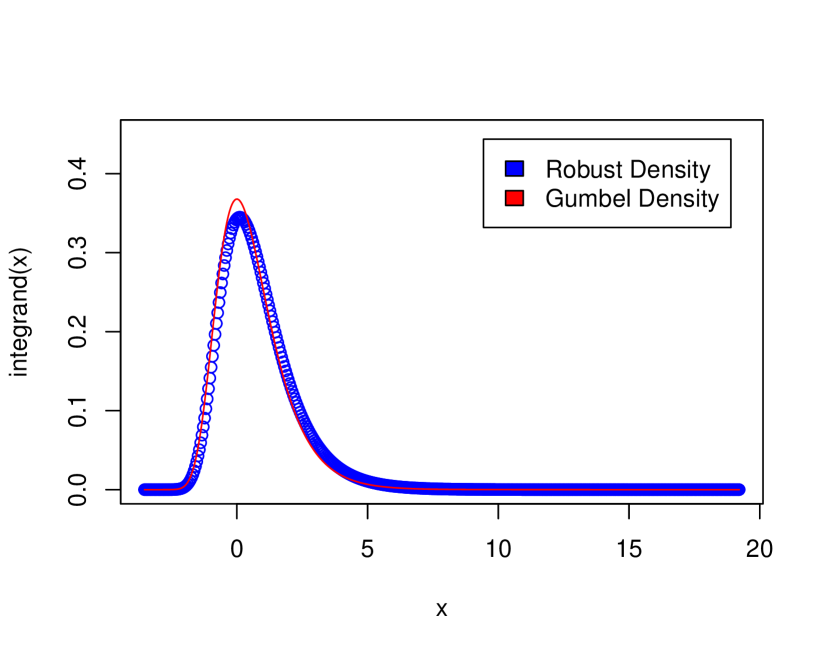
(a) $\rho=0.01$

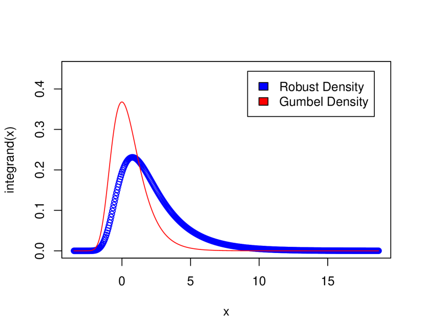
(b) $\rho=0.5$

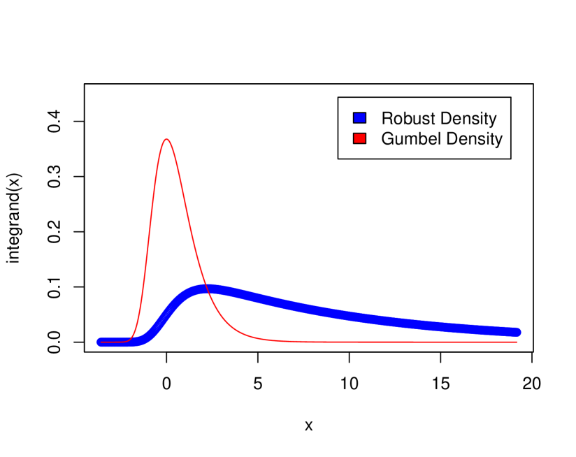
(c) $\rho=3.5$

Figure 1: Three instances of $\rho$

The result in Lemma 3 enables us to characterize the choice probability vector $p^{\star}(u)$ similarly to the celebrated WDZ theorem.

Theorem 1

Let Assumptions 1 and 2 hold. Let $\lambda^{\star}$ and $\mu^{\star}$ be the unique optimal solution to program (14), which induces $g^{\star}$ and $G^{\star}$ as the optimal density and distribution function, respectively. Then the following statements hold:

• The robust social surplus corresponds to the following:

  $$W^{DRO}(u)=\mathbb{E}_{G^{\star}}\left(\max_{j\in\mathcal{J}}\{u_{j}+\varepsilon_{j}\}\right)$$

• The choice probability vector $p^{\star}(u)$ is

  $$\nabla W^{DRO}(u)=p^{\star}(u).$$

Proof. (i) To show the first part, let us define the function $\Psi(\cdot)$ as follows $\Psi(\lambda,\mu)\triangleq\lambda\rho+\mu+\lambda\mathbb{E}_{F}\left(\phi^{*}\left({H(u,\varepsilon)-\mu\over\lambda}\right)\right)$. Optimizing $\Psi(\lambda,\mu)$ with respect to $\lambda$ and $\mu$ we get

$${\partial\Psi(\lambda,\mu)\over\partial\lambda} = \rho+\mathbb{E}_{F}\left(\phi^{*}\left({H(u,\varepsilon)-\mu\over\lambda}\right)\right)$$

$$+ \lambda\mathbb{E}_{F}\left(\phi^{\ast\prime}\left({H(u,\varepsilon)-\mu\over\lambda}\right)\left({H(u,\varepsilon)-\mu\over-\lambda^{2}}\right)\right)=0$$

$${\partial\Psi(\lambda,\mu)\over\partial\mu} = 1-\mathbb{E}_{F}\left(\phi^{\ast\prime}\left({H(u,\varepsilon)-\mu\over\lambda}\right)\right)=0$$

Rearranging the first equation, we have:

$$\lambda\rho+\lambda\mathbb{E}_{F}\left(\phi^{*}\left({H(u,\varepsilon)-\mu\over\lambda}\right)\right)+\mu\mathbb{E}_{F}\left(\phi^{\ast\prime}\left({H(u,\varepsilon)-\mu\over\lambda}\right)\right)$$

$$= \mathbb{E}_{F}\left(\phi^{\ast\prime}\left({H(u,\varepsilon)-\mu\over\lambda}\right)H(u,\varepsilon)\right).$$

Similarly, in the second equation, we have:

$$\mathbb{E}_{F}\left(\phi^{\ast\prime}\left({H(u,\varepsilon)-\mu\over\lambda}\right)\right)=1$$

Combining both expressions we find that the optimal $\lambda^{\star}$ and $\mu^{\star}$ must satisfy:

$$\lambda^{\star}\rho+\lambda^{\star}\mathbb{E}_{F}\left(\phi^{*}\left({H(u,\varepsilon)-\mu^{\star}\over\lambda^{\star}}\right)\right)+\mu^{\star}=\mathbb{E}_{F}\left(\phi^{\ast\prime}\left({H(u,\varepsilon)-\mu^{\star}\over\lambda^{\star}}\right)H(u,\varepsilon)\right).$$

Using expression (20) in Lemma 3, we obtain:

$$\Psi(\lambda^{\star},\mu^{\star})=\mathbb{E}_{F}\left(\phi^{\ast\prime}\left({H(u,\varepsilon)-\mu^{\star}\over\lambda^{\star}}\right)H(u,\varepsilon)\right)=\mathbb{E}_{G^{\star}}\left(\max_{j\in\mathcal{J}}\{u_{j}+\varepsilon_{j}\}\right).$$

Hence, we conclude that

$$W^{DRO}(u)=\mathbb{E}_{G^{\star}}\left(\max_{j\in J}\{u_{j}+\varepsilon_{j}\}\right).$$

(ii) To show that $\nabla W^{DRO}(u)=p^{\star}(u)$, we note that using the optimized value $\Psi(\lambda^{\star},\mu^{\star})=\lambda^{\star}\rho+\mu^{\star}+\lambda^{\star}\mathbb{E}_{F}\left(\phi^{*}\left({H(u,\varepsilon)-\mu^{\star}\over\lambda^{\star}}\right)\right)$ we get:

$${\partial W^{DRO}(u)\over\partial u_{j}} = {\partial\Psi(\lambda^{\star},\mu^{\star})\over\partial u_{j}}$$

$$= \int_{\varepsilon\in\mathbb{R}^{J+1}}\left(\phi^{\ast\prime}\left({H(u,\varepsilon)-\mu^{\star}\over\lambda^{\star}}\right){\partial H(u,\varepsilon)\over\partial u_{j}}\right)f(\varepsilon)d\varepsilon$$

$$= \mathbb{E}_{G^{\star}}\left({\partial H(u,\varepsilon)\over\partial u_{j}}\right)$$

$$= p^{\star}_{j}(u).$$

As previous result holds for all $j\in\mathcal{J}$, we conclude that $\nabla W^{DRO}(u)=p^{\star}(u)$.   $\square$

Part (i) of the theorem establishes that given the optimal solutions $\lambda^{\star}$ and $\mu^{\star}$, the surplus function $W^{DRO}(u)$ takes the familiar expected maximum form that characterizes the RUM (see Eq.(2)). The main difference between the characterization in part (i) and the surplus functions from RUM is that expression ((i)) corresponds to the expectation with respect to the robust distribution $G^{\star}$. Part (ii) shows that the gradient of $W^{DRO}(u)$ yields the choice probability vector $p^{\star}(u)$. This latter result generalizes the WDZ to environments where the nominal distribution $F$ may be misspecified or incorrect. In other words, Theorem 1 shows that the DRO-RUM preserves the expected maximum form and the gradient structure of the popular RUM.

4 Empirical content of the DRO-RUM

In this section, we discuss the empirical content of the DRO-RUM. In particular, we show how our approach is suitable to recover the mean utility vector allowing for uncertainty about the true distribution generating $\varepsilon$.

To gain some intuition, consider a situation where the choice probability vector $p$ is observed from market data. Then the analyst’s goal is to find a vector $u$ that rationalizes the observed $p$. Following Berry (1994), this problem is known as the demand inversion. In particular, Berry (1994) shows that in the case of the MNL $u$ satisfy the following

$$p_{j}={e^{u_{j}}\over 1+\sum_{j^{\prime}=1}^{J}e^{u_{j^{\prime}}}}\quad\mbox{for $j=1,\ldots,J.$}$$

and

$$p_{0}={1\over 1+\sum_{j^{\prime}=1}^{J}e^{u_{j^{\prime}}}}$$

Then using the previous expressions, we can solve for the mean utility vector $u$ as a function of $p$:

$$\log(p_{j}/p_{0})=u_{j}\quad\mbox{for $j=1,\ldots,J$}.$$

In other words, we can express $u$ in terms of the observed choice probability vector $p$.

We can use a similar argument to find the vector $u$ in the case of the nested logit, the random coefficient MNL model (Berry (1994); Berry et al. (1995)), and in the case of the inverse product differentiation logit model of Fosgerau et al. (2022). For general RUMs beyond the MNL and its variants, Galichon and Salanié (2021) develops a general approach based on convex duality and mass transportation techniques. They show that for any fixed distribution of $\varepsilon$ the mean utility vector $u$ is identified from the observed choice probability $p$.

This section aims to show that the DRO-RUM can be used to study the demand inversion problem in environments where the analyst does not know the true distribution of $\varepsilon$. Thus, our approach allows us to identify $u$ under misspecification of the distribution governing the realizations of $\varepsilon$.

4.1 Robust demand inversion

Our main result uses a distributionally robust version of the Fenchel equality for discrete choice models. In order to establish this result, we define $\mathcal{U}\triangleq\{u\in\mathbb{R}^{J+1}:u_{0}=0\}$. In other words, $\mathcal{U}$ is the set of mean utility vectors with the normalization $u_{0}=0$ for the outside option. Our first step is to understand the properties of the convex conjugate of $W^{DRO}(u)$:

$${W^{(DRO)}}^{*}(p)=\sup_{u\in\mathcal{U}}\left\{\langle u,p\rangle-W^{DRO}(u)\right\}.$$ (27)

In particular, we are interested in understanding the behavior of $W^{(DRO)^{*}}(p)$ on its effective domain of:

$$\mbox{dom}\,{W^{(DRO)}}^{*}=\left\{p\in\mathbb{R}^{J+1}\,|\,{W^{DRO}}^{*}(p)<\infty\right\}.$$

The following lemma plays a key role in our analysis.

Lemma 4

Let Assumptions 1 and 2 hold. Then $W^{DRO}(u)$ is strictly convex in $u$.

Proof. For given $\lambda$ and $\mu$, for $u_{1},u_{2}$ and $\alpha\in\left(0,1\right)$ we have

$$\lambda\mathbb{E}_{F}\left(\phi^{*}\left({H(\alpha u_{1}+\left(1-\alpha\right)u_{2},\varepsilon)-\mu\over\lambda}\right)\right)$$

$$\overset{(\star)}{\leq}\lambda \mathbb{E}_{F}\left(\phi^{*}\left({\alpha H(u_{1},\varepsilon)+\left(1-\alpha\right)H(u_{2},\varepsilon)-\mu\over\lambda}\right)\right),$$

where $\left(\star\right)$ holds due to the convexity of $H$ and the monotonicity of $\phi^{*}$ due to Assumption 2. Exploiting the strict convexity of $\phi^{*}$ and the linearity and monotonicity of the expectation operator further yields:

$$\lambda\mathbb{E}_{F}\left(\phi^{*}\left({\alpha H(u_{1},\varepsilon)+\left(1-\alpha\right)H(u_{2},\varepsilon)-\mu\over\lambda}\right)\right)$$

$$<\, \alpha\lambda\mathbb{E}_{F}\left(\phi^{*}\left({H(u_{1},\varepsilon)-\mu\over\lambda}\right)\right)+\left(1-\alpha\right)\lambda\mathbb{E}_{F}\left(\phi^{*}\left({H(u_{2},\varepsilon)-\mu\over\lambda}\right)\right).$$

Thus it follows that $W^{DRO}(u)$ is strictly convex in $u$.   $\square$

The following theorem establishes the continuity and smoothness of $W^{(DRO)^{*}}$.

Theorem 2

Let Assumptions 1 and 2 hold. The convex conjugate $W^{(DRO)^{*}}$ is continuous on its domain $\mbox{dom}\,{W^{(DRO)}}^{*}$ which coincides with the probability simplex $\Delta_{J+1}$. Furthermore, $W^{(DRO)^{*}}$ is continuously differentiable on $\mbox{int dom}\,W^{(DRO)^{*}}$.

Proof.  Let us first show that $\mbox{dom}\,{W^{(DRO)}}^{*}\subseteq\Delta_{J+1}$. Fix a utility vector $\bar{u}$ and take any $p\in\mathbb{R}^{J+1}$ with $\langle p,e\rangle\neq 1$. Then, using Lemma1(iii) we have

$${W^{(DRO)}}^{*}(p)\geq\sup_{\gamma\in\mathbb{R}}\langle p,\bar{u}+\gamma\cdot e\rangle-{W^{DRO}}(\bar{u}+\gamma\cdot e)$$

$$\overset{(iii)}{=} \langle p,\bar{u}\rangle-{W^{DRO}}(\bar{u})+\sup_{\gamma\in\mathbb{R}}\gamma\left(\langle e,p\rangle-1\right)=\infty.$$

Next, we take any vector $p\in\mathbb{R}^{J+1}$ with $p_{i}<0$ for some $i\in\left\{0,1,\ldots,J\right\}$. By Lemma 1 (ii), it follows that

$${W^{(DRO)}}^{*}(p)\geq\sup_{\gamma<0}\langle p,\gamma\cdot e_{i}\rangle-{W^{DRO}}(e_{i})\overset{(ii)}{\geq}\sup_{\gamma<0}\gamma\cdot p_{i},-{W^{DRO}}(0)=\infty.$$

Hence, it remains to prove the reverse implication, i. e. $\Delta_{J+1}\subseteq\mbox{dom}\,{W^{(DRO)}}^{*}$. Therefore, we derive an upper bound for the convex conjugate on the simplex:

$$\sup_{p\in\Delta_{J+1}}{W^{(DRO)}}^{*}(p)=\sup_{p\in\Delta_{J+1}}\left(\sup_{u\in\mathcal{U}}\langle p,u\rangle-W^{DRO}(u)\right)$$

$$= \sup_{u\in\mathcal{U}}\left(\sup_{p\in\Delta_{J+1}}\langle p,u\rangle-W^{DRO}(u)\right).$$

We apply (iii) from Lemma 1 which yields

$$\sup_{u\in\mathcal{U}}\left(\sup_{p\in\Delta_{J+1}}\langle p,u\rangle-W^{DRO}(u)\right)=\sup_{u\in\mathcal{U}}\left(\max_{i\in\mathcal{J}}u_{i}-W^{DRO}(u)\right)\leq-\min_{i\in\mathcal{J}}\mathbb{E}_{F}\left[\varepsilon_{i}\right].$$

Thus, the domain coincides with the simplex. For the continuity, we first observe that ${W^{(DRO)}}^{*}$ is convex, and hence it is continuous on the relative interior of its domain. The Gale-Klee-Rockafellar theorem provides upper semi-continuity of ${W^{(DRO)}}^{*}$ if the domain is polyhedral, which it is (Rockafellar, 1970). Furthermore, convex conjugates are always lower semi-continuous, and hence continuity follows. In order to establish that $W^{(DRO)^{*}}$ is continuously differentiable, we note that Lemma 4 shows that $W^{(DRO)^{*}}$ is strictly convex in $u$. Then by Hiriart-Urruty and Lemarechal (1993, Thm. 4.1.1) we know that the strict convexity of $W^{DRO}(u)$ implies that $W^{(DRO)^{*}}(p)$ is continuously differentiable on $\mbox{int}\left(\mbox{dom}\,W^{(DRO)^{*}}\right)$.   $\square$

The previous result is key in our goal of identifying the mean utilities. To see this we note that thanks to Theorem 1 we know that for alternative $j\in\mathcal{J}$ :

$$p_{j}={\partial W^{DRO}(u)\over\partial u_{j}}$$

Furthermore, from Theorem 2 we get:

$$u_{j}={\partial W^{(DRO)^{*}}(p)\over\partial p_{j}}$$

where $u$ achieves the maximum in (27). Then by Fenchel’s duality theorem, we know that these two conditions are equivalent. Then, given the robust distribution $G^{\star}$, we conclude that $u$ is identified from $p$. In other words, we can find a vector $u$ that rationalizes the observed choice probability vector $p$.

The following result establishes the empirical content of the DRO-RUM.

Theorem 3

Let Assumptions 1 and 2 hold. Then, the following statements are equivalent:

• The choice probability vector $p\in\Delta_{J+1}$ satisfies:

  $$p=\nabla W^{DRO}(u).$$ (28)

• The deterministic utility vector $u\in\mathcal{U}$ satisfies:

  $$u=\nabla W^{(DRO)^{*}}(p).$$ (29)

• $(u^{\star},\lambda^{\star},\mu^{\star})$ is the unique solution to the strictly convex optimization problem:

  $$-W^{(DRO)^{\ast}}(p)=\inf_{u\in\mathcal{U},\lambda\in\mathbb{R}_{+},\mu\in\mathbb{R}}\left\{\lambda\rho+\mu+\lambda\mathbb{E}_{F}\left(\phi^{*}\left({H(u,\varepsilon)-\mu\over\lambda}\right)\right)-\langle p,u\rangle\right\}.$$ (30)

Proof. The equivalence of parts (i) and (ii) follows from Theorem 2, which allows us to invoke Fenchel equality to conclude the result. To show part (iii), let us look at $W^{(DRO)^{*}}(p)$. By definition, we know that

$$W^{(DRO)^{*}}(p)=\sup_{u\in\mathcal{U}}\{\langle p,u\rangle-W^{DRO}(u)\}.$$

Proposition 2 implies that the previous expression corresponds to

$$W^{(DRO)^{*}}(p)=\sup_{u\in\mathcal{U}}\left\{\langle p,u\rangle-\inf_{\lambda>0,\mu\in\mathbb{R}}\left\{\lambda\rho+\mu+\lambda\mathbb{E}_{F}\left(\phi^{*}\left({H(u,\varepsilon)-\mu\over\lambda}\right)\right)\right\}\right\}.$$

Equivalently, we have:

$$W^{(DRO)^{*}}(p)=-\inf_{u\in\mathcal{U},\lambda>0,\mu\in\mathbb{R}}\left\{\lambda\rho+\mu+\lambda\mathbb{E}_{F}\left(\phi^{*}\left({H(u,\varepsilon)-\mu\over\lambda}\right)\right)-\langle p,u\rangle\right\}.$$

Thus, we get:

$$-W^{(DRO)^{*}}(p)=\inf_{u\in\mathcal{U},\lambda>0,\mu\in\mathbb{R}}\left\{\lambda\rho+\mu+\lambda\mathbb{E}_{F}\left(\phi^{*}\left({H(u,\varepsilon)-\mu\over\lambda}\right)\right)-\langle p,u\rangle\right\}.$$

Combining Lemmas 2 and 4 we get that the (30) is strictly convex in $u,\lambda,$ and $\mu$. As a consequence, there exists a unique solution to the problem (30).  $\square$

As we discussed in the introduction of this section, for a fixed distribution of $\varepsilon$, parts (i) and (ii) have been established in the Galichon and Salanié (2021). Our result differs from theirs in a fundamental aspect; we achieve the identification of the mean utility vector $u$, relaxing the assumption that the distribution of $\varepsilon$ is known. In other words, our result allows for nonparametric identification of $u$ under (potential) misspecification of the shock distribution. Similarly, our result relates to dynamic discrete choice models’ “inversion” approach. For instance the papers by Hotz and Miller (1993) and Arcidiacono and Miller (2011) establish that the mean utility vector $u$ can be recovered as $\nabla^{-1}W(p)=u$. Their approach only applies to the case of the MNL and GEV models. By exploiting convex optimization techniques, Fosgerau et al. (2021) extends Hotz and Miller (1993) and Arcidiacono and Miller (2011)’s inversion approach to models far beyond the GEV class. Similarly, Li (2018) considers a convex minimization algorithm to solve the demand inversion problem. He illustrates his method in the case of both the Berry et al. (1995) random coefficient logit demand model and the Berry and Pakes (2007) pure characteristics model. However, Fosgerau et al. (2021) and Li (2018)’s results only apply under the assumption that the distribution of $\varepsilon$ is known. In contrast, part (iii) establishes that given a choice probability vector $p$, we can identify the mean utility vector $u$ as the unique solution of the strictly convex optimization program (30). This latter characterization captures the role of misspecification through the value of the Lagrange multipliers $\lambda^{\star}$ and $\mu^{\star}$. Thus, Theorem 3 provides a distributionally robust nonparametric identification result.

4.2 A robust random coefficient model

To see how Theorem 3 can be applied, we analyze the random coefficient model assuming that the $\phi$-divergence corresponds to the Kullback-Leibler distance. Following Berry et al. (1995) and Galichon and Salanié (2021), we consider a random coefficient model with $\varepsilon=Ze+T\eta$, where $e$ is a random vector on $\mathbb{R}^{k}$ with distribution $F_{e}$ , $Z$ is a $\left|\mathcal{J}\right|\times k$ matrix, $T>0$ is a scalar parameter, and $\eta$ is a vector of $|\mathcal{J}|$ Gumbel random variables, whose distribution function is $F_{\eta}$. Assume that $e$ and $\eta$ are statistically independent. Fixing the distributions $F_{e}$ and $F_{\eta}$, we can use the iterated expectation, combined with the independence of $e$ and $\eta$ ((Galichon and Salanié, 2021, Eqs. B.6-B.7)) we get that

$$W(u) = \mathbb{E}_{F_{e}}\left(\mathbb{E}_{\eta}\left(\max_{j\in\mathcal{J}}\{u_{j}+(Ze)_{j}+T\eta_{j}\}\right)|e\right),$$

$$= \mathbb{E}_{F_{e}}\left(W(u+Ze)\right),$$

where $W(u+Ze)=\int_{\mathbb{R}^{J+1}}\max_{j\in\mathcal{J}}\{u_{j}+(Ze)_{j}+T\eta_{j}\}f_{\eta}d\eta$. Using the fact that $\eta$ follows a Gumbel distribution, we find that

$$W(u+Ze)=T\log\left(\sum_{j\in\mathcal{J}}{e^{u_{j}+(Ze)_{j}\over T}}\right).$$

Let us assume that $F_{e}$ approximates the true distribution generating $e$. Then we can define $W^{DRO}(u)$ as follows:

$$W^{DRO}(u)=\sup_{G_{e}\in\mathcal{M}_{\phi}(F_{e})}\mathbb{E}_{G_{e}}\left(T\log\left(\sum_{j\in\mathcal{J}}e^{{u_{j}+(Ze)_{j}\over T}}\right)\right)$$

To apply Theorem 3, we note that $H(u,\varepsilon)=T\log\left(\sum_{j\in\mathcal{J}}e^{{u_{j}+(Ze)_{j}\over T}}\right)$. Then, using the Kullback-Leibler distance, we have that for an observable choice probability vector $p$, the identified mean utility vector $u^{\star}$ corresponds to the solution of the following program:

$$-W^{(DRO)^{\ast}}(p)=\inf_{u\in\mathcal{U},\lambda>0}\left\{\rho\lambda+\lambda\ln\mathbb{E}_{F_{e}}\|e^{u+Ze}\|_{T^{-1}}-\langle p,u\rangle\right\},$$ (31)

where $\|e^{u+Ze}\|_{T^{-1}}\triangleq\left(\sum_{j\in\mathcal{J}}e^{{u_{j}+(Ze)_{j}\over T}}\right)^{T}.$

The program (31) allows us to identify the mean utility vector enabling some degree of misspecification in the distribution of $e$. It is worth remarking that program (31) is fairly tractable, so we can use traditional stochastic programming algorithms to find its unique solution.

5 Numerical Experiments

In this section, we discuss numerical simulations of our approach. We compare the DRO-RUM with the MNL and MNP models.

Our main goal is to analyze the effect of the robustness index $\rho$ on the choice probabilities. We consider a scenario with four alternatives where $\mathcal{J}=\{0,1,2,3\}$. Our first parametrization of the utility vector $u$ is $u=\left(0,1,2,2.1\right)^{T}$. Based on this specification, we proceed to calculate the choice probabilities. In the case of the MNL, the choice probabilities are computed via Eq. (4) , where the scale parameter equals one ( $\eta=1$). In addition, we set the location parameter of each Gumbel error is assumed to zero. For the MNP, we consider two different parametrizations for the variance-covariance matrix of the random error vectors; $\mathcal{N}(0,\Sigma_{1})$ and $\mathcal{N}(0,\Sigma_{2})$ where

$$\Sigma_{1}=\left(\begin{array}[]{ccccc}1&0&0&0\\ 0&1&0&0\\ 0&0&1&0\\ 0&0&0&1\\ \end{array}\right),\qquad\Sigma_{2}=\left(\begin{array}[]{ccccc}2&-0.5&0.5&1.3\\ -0.5&2&0&0.15\\ 0.5&0&2&1\\ 1.3&0.15&1&2\\ \end{array}\right).$$

We call the latter model MNP-dep and the former MNP-indep, as the random errors $\varepsilon^{(i)}$, $i=1,\ldots,4$ are independent in the former model. We use 10,000,000 draws from the error vectors to stabilize the simulations to simulate the choice probabilities.
For the DRO-RUMs, we choose the Kulback-Leibler- divergence case presented in Example 1. We assume that the error terms of the nominal distribution are iid Gumbel distributed with location parameter zero and scale parameter one. This yields a way to examine the behavior and numerical stability of the DRO-RUM, and the impact of $\rho$ on the choice probabilities.

The robust choice probabilities are simulated similarly to the MNP models. However, for the case of DRO-RUM we have to generate samples from the distribution defined by the density 25. First, the optimal $\lambda^{\star}$ in (24) as well as $\mathbb{E}_{F}\left(e^{H(u,\varepsilon)/\lambda^{\star}}\right)$ are estimated using $50,000,000$ simulations from $4$ iid Gumbel distributions. Based on the optimized parameters a higher dimensional acceptance-rejection algorithm provides an efficient sampling method. For performance, the code was written in Julia.

We present the results in Table 2

	Alternative $1$	Alternative $2$	Alternative $3$	Alternative $4$
MNL	$5.1885\%$	$14.1037\%$	$38.3379\%$	$42.3699\%$
MNP-indep	$1.6243\%$	$10.2996\%$	$41.443\%$	$46.6331\%$
MNP-dep	$1.7877\%$	$19.359\%$	$37.9993\%$	$40.854\%$
$\rho=0.1$	$9.2391\%$	$18.4783\%$	$33.695\%$	$38.587\%$
$\rho=0.7$	$13.2132\%$	$19.7823\%$	$31.6066\%$	$35.3979\%$
$\rho=1.3$	$15.4725\%$	$21.5501\%$	$30.5269\%$	$32.4505\%$
$\rho=2.2$	$18.1501\%$	$21.46\%$	$29.7536\%$	$30.6363\%$
$\rho=4.3$	$21.5843\%$	$23.2006\%$	$27.1235\%$	$28.0916\%$

Table 2: Choice Probabilities for utility vector $u=\left(0,1,2,2.1\right)^{T}$

.

In the previous table, the first row displays the choice probability for the MNL. The second and third rows show the choice probabilities for the MNP-indep and MNP-dep. The fourth row shows the behavior of the DRO-RUM when $\rho=0.1$. For this parametrization, the DRO-RUM yields choice probabilities that are similar (not equal) to the ones displayed by the MNP-dep. Similar behavior is observed for the case of $\rho=0.7$.

Rows six to eight show the behavior of the DRO-RUM as we increase $\rho$. As expected, as the value of $\rho$ increases, the choice probabilities look similar to the uniform choice between alternatives. In particular, for the case of $\rho=4.3$ we note that DRO-RUM assigns probabilities similar to the uniform case. Intuitively, a large $\rho$ , represents a situation where the analyst is highly uncertain about the true distribution. Thus, her behavior is overly cautious and considers a large set of possible (and feasible) distributions. Hence, when $\rho\longrightarrow\infty$, the analyst’s best choice is to guess uniform probabilities.

Similarly, from the DM’s perspective, large values of $\rho$ indicate a cautious and flexible choice of the error term. Consequently, the random error term might follow a distribution that completely counteracts the deterministic utilities’ effects and guarantees the same overall random utility for every alternative. Indeed, the robust surplus function (23) is strongly increasing with a larger index of robustness as shown in Figure 2, where we plot the surplus function evaluated at $u=\left(0,1,2,2.1\right)^{T}$ for different values of $\rho$.

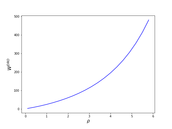
Figure 2: Robust surplus $W^{DRO}$ for the utility vector $u$ and different values of robustness index $\rho$.

A well-known pitfall of the MNL model is that it satisfies the independence of irrelevant alternatives (IIA) property. The IIA property establishes that the ratio between the probabilities of any two alternatives only depends on the differences between the utilities of these two alternatives. This property follows directly via formula (4). A direct implication of this fact is that when the deterministic utility of one alternative changes, the choice probabilities change proportionally so that the probability ratio between alternatives remains constant. In contrast, the DRO-RUM incorporates some dependence structure into the MNL. Hence, it is interesting to simulate choice probabilities for a slight change in the deterministic utility vector. In Table 3, we summarize the choice the probabilities for the alternatives with utility vector $\tilde{u}=\left(0,1,2,2.2\right)^{T}$.

	Alternative $1$	Alternative $2$	Alternative $3$	Alternative $4$
MNL	$4.9671\%$	$13.5021\%$	$36.7024\%$	$44.8284\%$
MNP-indep	$1.4758\%$	$9.5821\%$	$39.2676\%$	$49.6745\%$
MNP-dep	$1.5544\%$	$18.5851\%$	$36.0749\%$	$43.7856\%$
$\rho=0.1$	$6.8788\%$	$15.0473\%$	$36.5434\%$	$41.5305\%$
$\rho=0.7$	$13.2076\%$	$20.2437\%$	$30.8569\%$	$35.6918\%$
$\rho=1.3$	$15.2938\%$	$21.5069\%$	$30.7281\%$	$32.4712\%$
$\rho=2.2$	$17.9704\%$	$21.4406\%$	$29.5254\%$	$31.0636\%$
$\rho=4.3$	$21.5509\%$	$23.264\%$	$27.4421\%$	$27.743\%$

Table 3: Choice Probabilities for utility vector $\tilde{u}=\left(0,1,2,2.2\right)^{T}$

The violation of IIA, is visualized in Figure 3. Note that in the MNL, the decrease in choosing alternative $4$ evenly increases the probability of choosing one of the alternatives $1-3$, indicated by the dotted line. At the same time, the substitution patterns for the robust models are way more flexible.

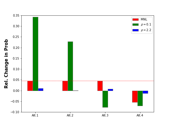
Figure 3: Relative change in probabilities if deterministic utility vector changes from $\tilde{u}$ to $u$.

6 Final remarks

In this paper, we have introduced the DRO-RUM, which allows the shock distribution to be unknown or misspecified. We have shown that the DRO-RUM preserves the tractability and convex structure of the traditional RUM. Furthermore, we characterized the empirical content of the DRO-RUM, establishing that for an observed choice probability vector, there exists a unique mean utility vector that rationalizes the observed behavior in terms of a DRO-RUM. Finally, we showed the stability and numerical properties of our approach.

Several extensions are possible. First, a natural question is about the econometric performance of the DRO-RUM using market data. This is in particular interesting, as our our approach provides the analyst with a rich class of various models. In fact, different models can be created by simply choosing a different $\phi$ - divergence and/or nominal distribution. In this context, it is also interesting to examine the impact of the robustness parameter $\rho$.

Second, results of RUM could be analyzed in the framework of robustness. For instance, the results in this paper could help study two-sided matching markets with transferable utility. Similarly, our results can help study robust identification in dynamic discrete choice models.

The algorithmic aspects of the DRO-RUM could be analyzed. Recently for example, a new family of prox-functions on the probability simplex based on discrete choice models has been introduced by Müller et al. (2022). Hence, it is interesting to see if prox-functions can be generated from the DRO-RUM.

Additionally, theoretical extensions of the distributionally robust approach are conceivable. A natural way to do this is to rely on different statistical distance concepts, e.  g. Wasserstein-Distance, and analyze their tractability. Moreover, the properties of such other robust models could be compared with the DRO-RUM.

References

- Arcidiacono and Miller (2011) Peter Arcidiacono and Robert A. Miller. Conditional choice probability estimation of dynamic discrete choice models with unobserved heterogeneity. Econometrica, 79(6):1823–1867, 2011.
- Becker et al. (1963) Gordon M. Becker, Morris H. Degroot, and Jacob Marschak. Stochastic models of choice behavior. Behavioral Science, 8(1):41–55, 1963.
- Ben-Tal and Teboulle (1987) A. Ben-Tal and M. Teboulle. Penalty functions and duality in stochastic programming via -divergence functionals. Mathematics of Operations Research, 12(2):224–240, 1987.
- Berry and Pakes (2007) Steven Berry and Ariel Pakes. The pure characteristics demand model. International Economic Review, 48(4):1193–1225, 2007.
- Berry et al. (1995) Steven Berry, James Levinsohn, and Ariel Pakes. Automobile prices in market equilibrium. Econometrica, 63(4):841–890, 1995.
- Berry (1994) Steven T. Berry. Estimating discrete-choice models of product differentiation. The RAND Journal of Economics, 25(2):242–262, 1994. ISSN 07416261.
- Block and Marschak (1959) H.D. Block and Jacob Marschak. Random orderings and stochastic theories of response. Cowles Foundation Discussion Papers 66, Cowles Foundation for Research in Economics, Yale University, 1959.
- Chiong et al. (2016) Khai Xiang Chiong, Alfred Galichon, and Matt Shum. Duality in dynamic discrete-choice models. Quantitative Economics, 7(1):83–115, 2016.
- Christensen and Connault (2023) Timothy Christensen and Benjamin Connault. Counterfactual sensitivity and robustness. Econometrica, 91(1):263–298, 2023.
- Csiszar (1967) I. Csiszar. Information-type measures of difference of probability distributions and indirect observation. Studia Scientiarum Mathematicarum Hungarica, 2:229–318, 1967.
- Dacorogna and Maréchal (2008) Bernard Dacorogna and Pierre Maréchal. The role of perspective functions in convexity, polyconvexity, rank-one convexity and separate convexity. Journal of convex analysis, 15(ARTICLE):271–284, 2008.
- Feng et al. (2017) Guiyun Feng, Xiaobo Li, and Zizhuo Wang. Technical note—on the relation between several discrete choice models. Operations Research, 65(6):1516–1525, 2017.
- Fosgerau et al. (2021) Mogens Fosgerau, Emerson Melo, Matthew Shum, and Jesper R.-V. Sørensen. Some remarks on ccp-based estimators of dynamic models. Economics Letters, 204:109911, 2021. ISSN 0165-1765.
- Fosgerau et al. (2022) Mogens Fosgerau, Julien Monardo, and Andre de Palma. The inverse product differentiation logit model. Working paper, 2022.
- Galichon and Salanié (2021) Alfred Galichon and Bernard Salanié. Cupid’s Invisible Hand: Social Surplus and Identification in Matching Models. The Review of Economic Studies, 89(5):2600–2629, 12 2021. ISSN 0034-6527.
- Hansen and Sargent (2001) Lars Peter Hansen and Thomas J. Sargent. Robust control and model uncertainty. The American Economic Review, 91(2):60–66, 2001. ISSN 00028282.
- Hansen and Sargent (2008) Lars Peter Hansen and Thomas J. Sargent. Robustness. Princeton University Press, stu - student edition edition, 2008.
- Hiriart-Urruty and Lemarechal (1993) Jean-Baptiste Hiriart-Urruty and Claude Lemarechal. Convex Analysis and Minimization Algorithms II. Addison-Wesley Professional, 2 edition, 1993.
- Hotz and Miller (1993) V. Joseph Hotz and Robert A. Miller. Conditional Choice Probabilities and the Estimation of Dynamic Models. The Review of Economic Studies, 60(3):497–529, 07 1993. ISSN 0034-6527.
- Hu and Hong (2012) Zhaolin Hu and L. Jeff Hong. Kullback-leibler divergence constrained distributionally robust optimization. Working Paper, 2012.
- Kuhn et al. (2019) Daniel Kuhn, Peyman Mohajerin Esfahani, Viet Anh Nguyen, and Soroosh Shafieezadeh-Abadeh. Wasserstein Distributionally Robust Optimization: Theory and Applications in Machine Learning, chapter 6, pages 130–166. 2019.
- Li (2018) Lixiong Li. A general method for demand inversion, 2018.
- Liese and Vajda (1987) F. Liese and I. Vajda. Convex statistical distances. Leipzig: Teubner-Texte zur Mathematik, Band 95., 1987.
- Marschak (1959) Jacob Marschak. Binary choice constraints on random utility indicators. Technical report, 1959.
- McFadden (1978a) D. McFadden. Modeling the choice of residential location. in A. Karlqvis, A., Lundqvist, L., Snickars, L., Weibull, J. (eds.), Spatial Intearction Theory and Planning Models (North Holland, Amsterdam), pages 531–551, 1978a.
- McFadden (1978b) D. McFadden. Modeling the choice of residential location. Transportation Research Record, (673):72–77, 1978b.
- McFadden (1978c) D. McFadden. Spatial interaction theory and residential location, chapter : Modeling the choice of residential location, pages 75–96. North-Holland, Amsterdam, 1978c.
- McFadden (1981) D. McFadden. Structural Analysis of Discrete Data with Econometric Applications, chapter : Econometric Models of Probabilistic Choice, pages 198–272. Cambridge: MIT, 1981.
- McFadden (2001) Daniel McFadden. Economic choices. American Economic Review, 91(3):351–378, June 2001.
- Mishra et al. (2012) Vinit Kumar Mishra, Karthik Natarajan, Hua Tao, and Chung-Piaw Teo. Choice prediction with semidefinite optimization when utilities are correlated. IEEE Transactions on Automatic Control, 57(10):2450–2463, 2012.
- Mishra et al. (2014) Vinit Kumar Mishra, Karthik Natarajan, Dhanesh Padmanabhan, Chung-Piaw Teo, and Xiaobo Li. On theoretical and empirical aspects of marginal distribution choice models. Management Science, 60(6):1511–1531, 2014.
- Müller et al. (2022) David Müller, Yurii Nesterov, and Vladimir Shikhman. Discrete choice prox-functions on the simplex. Mathematics of Operations Research, 47(1):485–507, 2022.
- Natarajan et al. (2009) Karthik Natarajan, Miao Song, and Chung-Piaw Teo. Persistency model and its applications in choice modeling. Management Science, 55(3):453–469, 2009.
- Pardo (2005) L. Pardo. Statistical Inference Based on Divergence Measures. Chapman and Hall/CRC, 1 edition, 2005.
- Rockafellar (1976) R. Tyrrell Rockafellar. Integral functionals, normal integrands and measurable selections. In Jean Pierre Gossez, Enrique José Lami Dozo, Jean Mawhin, and Lucien Waelbroeck, editors, Nonlinear Operators and the Calculus of Variations, pages 157–207, Berlin, Heidelberg, 1976. Springer Berlin Heidelberg. ISBN 978-3-540-38075-7.
- Rockafellar (1970) T. R. Rockafellar. Convex Analysis. 1970.
- Ruszczyński and Shapiro (2021) Andrzej Ruszczyński and Alexander Shapiro. Lectures on Stochastic Programming: Modeling and Theory, Third Edition. 2021.
- Scarf (1958) H. Scarf. A min-max solution of an inventory problem. Studies in The Mathematical Theory of Inventory and Production, 1958.
- Shapiro (2017a) Alexander Shapiro. Distributionally robust stochastic programming. SIAM Journal on Optimization, 27(4):2258–2275, 2017a.
- Shapiro (2017b) Alexander Shapiro. Distributionally robust stochastic programming. SIAM Journal on Optimization, 27(4):2258–2275, 2017b.
- Train (2009) Kenneth E. Train. Discrete Choice Methods with Simulation. Cambridge University Press, 2 edition, 2009.