Finite Element Approximation of Data-Driven Problems in Conductivity

Abstract.

This paper is concerned with the finite element discretization of the data driven approach according to [19] for the solution of PDEs with a material law arising from measurement data. To simplify the setting, we focus on a scalar diffusion problem instead of a problem in elasticity. It is proven that the data convergence analysis from [9] carries over to the finite element discretization as long as $H(\operatorname{div})$-conforming finite elements such as the Raviart-Thomas element are used. As a corollary, minimizers of the discretized problems converge in data in the sense of [9], as the mesh size tends to zero and the approximation of the local material data set gets more and more accurate. We moreover present several heuristics for the solution of the discretized data driven problems, which is equivalent to a quadratic semi-assignment problem and therefore NP-hard. We test these heuristics by means of two examples and it turns out that the “classical” alternating projection method according to [19] is superior w.r.t. the ratio of accuracy and computational time.

1. Introduction

In material science, empirically developed material models are commonly in use, i.e., material laws that describe the behavior of materials are derived from measured data. But, due to measuring errors and simplified models, this approach bears the risk of inaccuracies. For this reason, an alternative data-driven concept has been established in [19]. In a sense, this concept skips the modeling step and uses the measured data directly. The idea is to select that data point from the set of measurements that best fits axiomatic physical laws such as first principles.

Let us explain this data-driven approach in terms of a stationary diffusion process of the form

$$-\operatorname{div}\kappa(\nabla u)=f\;\text{ in }\Omega,\quad u=0\;\text{ on }\Gamma:=\partial\Omega.$$ (1.1)

Here and in the following, $\Omega\subset\mathbb{R}^{d}$, $d\in\mathbb{N}$, is a bounded domain, $f\in H^{-1}(\Omega)\coloneqq H^{1}_{0}(\Omega)^{*}$, and $\operatorname{div}:L^{2}(\Omega;\mathbb{R}^{d})\to H^{-1}(\Omega)$ denotes the distributional divergence. Furthermore, $\kappa:\mathbb{R}^{d}\to\mathbb{R}^{d}$ is a given function which models the material law and is calibrated by $m\in\mathbb{N}$ measurements for the tuple $({\boldsymbol{q}},\nabla u)$ collected in the so-called local material data set

$$\mathcal{D}^{\textup{loc}}\coloneqq\{({\boldsymbol{r}}_{1},{\boldsymbol{w}}_{1}),\dots,({\boldsymbol{r}}_{m},{\boldsymbol{w}}_{m})\}\subset\mathbb{R}^{d}\times\mathbb{R}^{d}.$$ (1.2)

As indicated above, the idea is now to use these measurements directly. For this purpose, we rewrite (1.1) equivalently as

$$\eqref{SDP}\quad\Longleftrightarrow\quad({\boldsymbol{q}},\nabla u)\in\widetilde{\mathcal{D}}\times\mathcal{E},$$

with the so-called equilibirum set

$$\mathcal{E}\coloneqq\{({\boldsymbol{q}},\nabla u)\in L^{2}(\Omega;\mathbb{R}^{d})\times L^{2}(\Omega;\mathbb{R}^{d}):u\in H^{1}_{0}(\Omega),\;-\operatorname{div}\sigma=f\}$$ (1.3)

and the material law set

$$\widetilde{\mathcal{D}}\coloneqq\{({\boldsymbol{r}},{\boldsymbol{w}})\in L^{2}(\Omega;\mathbb{R}^{d})\times L^{2}(\Omega;\mathbb{R}^{d}):{\boldsymbol{r}}(x)=\kappa({\boldsymbol{w}}(x))\text{ a.e.\ in }\Omega\}.$$ (1.4)

The data-driven approach now skips the modelling step and uses the measured data directly by replacing $\widetilde{\mathcal{D}}$ with the material data set

$$\mathcal{D}\coloneqq\{({\boldsymbol{r}},{\boldsymbol{w}})\in L^{2}(\Omega;\mathbb{R}^{d})\times L^{2}(\Omega;\mathbb{R}^{d}):({\boldsymbol{r}},{\boldsymbol{w}})\in\mathcal{D}^{\textup{loc}}\text{ a.e.\ in }\Omega\}$$

where $\mathcal{D}^{\textup{loc}}$ is the collection of measurements from (1.2). Due to measurement errors and limited measuring capacities, the intersection $\mathcal{D}\cap\mathcal{E}$ is usually empty. One therefore resorts to a minimization problem of the form

$$\left.\begin{aligned} \min_{(y,z)\in Z\times Z}\quad&\|y-z\|_{Z}^{2}\\ \text{s.t.}\quad\quad&y\in\mathcal{D},\,z\in\mathcal{E},\end{aligned}\quad\right\}$$ (DDP)

i.e., one searches for two elements of the sets $\mathcal{E}$ and $\mathcal{D}$ that have smallest distance to each other. Herein, we abbreviated $Z:=L^{2}(\Omega;\mathbb{R}^{d})\times L^{2}(\Omega;\mathbb{R}^{d})$.

The optimization problem (DDP) is frequently called data-driven problem and gives rise to several questions and issues: First of all, while $\mathcal{E}$ is easily seen to be weakly closed, the set $\mathcal{D}$ is in general not. Hence, (DDP) does not necessarily admit a solution. Moreover, a natural question arising in context of (DDP) is its behavior for measurements getting more and more accurate. Does the arising data-driven limit recover the “true” material law and, if so, in which sense? Moreover, a numerical solution of (DDP) requires a discretization of (DDP) and one may ask how a discretization influences this data-driven limit. Finally, the material data set $\mathcal{D}$ involves a discrete point set such that (DDP) is a mixed-integer optimization problem. Problems of this type are typically hard to handle such that the development of efficient optimization algorithms for (DDP) (and its discretized counterpart) is all but trivial.

With this work, we address the two latter questions, i.e., we discuss discretization schemes and optimization algorithms for the solution of (DDP). Let us put our work into perspective. In engineering science, the data-driven approach is meanwhile well accepted and has been applied to various problems, in particular in solid mechanics, we only refer to [19, 20, 22, 12, 7] for examples from elasticity, inelasticity, dynamics, and fracture mechanics. A rigorous mathematical analysis of this approach has only been initiated recently in [9], where the concept of data convergence has been introduced. This notion of convergence is especially tailored to the structure of (DDP) and allows to characterize the data-driven limit. In this way, it answers the above question what happens, if the measurement errors tend to zero. The precise characterization of data-driven limits strongly depends on the particular structure of $\mathcal{D}$ and $\mathcal{E}$. This notion of convergence and the characterization of the associated limits have been investigated for several scenarios, we exemplarily refer to in [9, 10, 24]. To the best of our knowledge however, the discretization of $\mathcal{E}$ and $\mathcal{D}$ has not been incorporated into this convergence analysis so far and with this work, we aim to fill this gap. This is an important issue, not only because (DDP) cannot be solved in infinite dimensional spaces, but also due to the general lack of existence of solutions to (DDP). If one turns to a discretized counterpart of (DDP), then the finite dimensional structure allows to establish the existence of optimal solutions under mild assumptions so that, not until then, it makes sense to look for efficient algorithms for their computation.

As already indicated, the design of reliable and efficient solvers for (DDP) (and its discretization, respectively) is a delicate issue due to the discrete structure of the local material data set. In [19], a fixed-point type heuristic based on projections has been introduced, which is able to handle extensive measurement data, but may fail to converge or converges to spurious fixed-points that are not optimal, as shown in [18]. In the latter reference, a standard mixed-integer programming solver his employed to solve a data-driven problem of (unrealistically) small size. Due to the vast amount of measurement data, it is in principle impossible to use exact mixed-integer programming solvers for the solution of (DDP). Therefore, various heuristics have been developed and applied such as as kernel regression [16], local regression [17], tensor voting [13], and neural networks [23]. In the second part of the paper, we present some new heuristics and compare them with existing methods. Some of our algorithms are based on projection heuristic from [19], but we also tested a method, which employs an exact mixed-integer solver in combination with a local search algorithm.

We point out that we restrict ourselves to the conductivity example from (1.1) in order to keep the discussion as concise as possible. An extension of the finite element convergence analysis as well as the algorithmic approaches to problems in elasticity should be possible and is subject to future research.

The plan of the paper reads as follows: After introducing our standing assumptions and some well known results from saddle point theory in Section 2, we focus on the discretization of the equilibrium set by means of Raviart-Thomas type finite elements in Section 3. Afterwards, in Section 4, we recall the notion of data convergence from [9] and adapt it to our setting. Section 5 is then devoted to our main results, incorporating the finite element discretization of $\mathcal{E}$ and $\mathcal{D}$ into the data convergence analysis. In Section 6, we discuss the need for $H(\operatorname{div})$-conforming finite elements like the Raviart-Thomas element for the discretization of (DDP). Section 7 is dedicated to the algorithms and their implementation and finally, in Section 8, we present some numerical results.

2. Preliminaries and Standing Assumptions

As usual we define

$$H(\operatorname{div}):=\{{\boldsymbol{w}}\in L^{2}(\Omega;\mathbb{R}^{d})\colon\operatorname{div}{\boldsymbol{w}}\in L^{2}(\Omega)\},$$

where $\operatorname{div}:L^{2}(\Omega;\mathbb{R}^{d})\to H^{-1}(\Omega)$ denotes the distributional divergence. The following two lemmas concerning the space $H(\operatorname{div})$ will be useful in the rest of the paper. For their proofs, we refer to [26].

Lemma 2.1.

If the complement of $\overline{\Omega}$ satisfies the cone condition according to [26] , then $C^{\infty}(\overline{\Omega};\mathbb{R}^{d})$ is dense in $H(\operatorname{div})$.

Lemma 2.2.

Let $F\in H(\operatorname{div})^{*}$ and $f\in L^{2}(\Omega)$ be given. Then there exists a unique solution $({\boldsymbol{\tau}},\lambda)\in H(\operatorname{div})\times L^{2}(\Omega)$ to the saddle point problem

$$\int_{\Omega}{\boldsymbol{\tau}}\cdot{\boldsymbol{w}}\,dx+\int_{\Omega}\lambda\operatorname{div}{\boldsymbol{w}}\,dx \;=\; \langle F,{\boldsymbol{w}}\rangle\quad \forall\,{\boldsymbol{w}}\in H(\operatorname{div}),$$ (2.1a)

$$-\int_{\Omega}v\operatorname{div}{\boldsymbol{\tau}}\,dx =\; \int_{\Omega}fv\,dx\quad \forall v\in L^{2}(\Omega).$$ (2.1b)

If $\Omega$ satisfies the regularity assumptions from Lemma 2.1 and $F\in L^{2}(\Omega;\mathbb{R}^{d})$, then $\lambda\in H^{1}_{0}(\Omega)$. If moreover $\Omega$ is $H^{2}$-regular and $F\in H^{1}(\Omega;\mathbb{R}^{d})$, then ${\boldsymbol{\tau}}\in H^{1}(\Omega;\mathbb{R}^{d})$ and

$$\|{\boldsymbol{\tau}}\|_{H^{1}(\Omega;\mathbb{R}^{d})}\leq c(\|f\|_{L^{2}(\Omega)}+\|F\|_{H^{1}(\Omega;\mathbb{R}^{d})})$$

with a constant $c>0$, which only depends on $\Omega$.

Assumption 2.3.

Throughout this paper, we assume the following regularity assumptions on the domain and the inhomogeneity $f$:

1. The domain $\Omega$ is supposed to bounded and convex with a polygonal resp. polyhedral boundary.

2. The right-hand side in the divergence constraint satisfies $f\in L^{2}(\Omega)$.

Remark 2.4.

The regularity of the domain can be relaxed in the sense that we can drop the convexity, see Remark 3.9 below. In contrast to this, we need the higher regularity of $f$ and cannot work with inhomogeneities in $H^{-1}(\Omega)$, since our discretization requires $H(\operatorname{div})$-conforming finite elements as demonstrated in Section 6 below.

We underline that Assumption 2.3 is tacitly supposed to hold throughout the rest of the paper without mentioning it every time.

3. Discretization

The equilibrium constraint set $\mathcal{E}$ from (1.3) is discretized by

$$\mathcal{E}_{h}\coloneqq\{({\boldsymbol{q}}_{h},\nabla u_{h}):{\boldsymbol{q}}_{h}\in Q_{h},u_{h}\in U_{h},-\operatorname{div}_{h}{\boldsymbol{q}}_{h}=f\},$$ (3.1)

where $U_{h}$ and $Q_{h}$ are finite dimensional function spaces satisfying the following

Assumption 3.1.

The discretization of $\mathcal{E}$ in (3.1) is supposed to fulfill the following conditions:

1. For all $h>0$, the discrete spaces $U_{h}$ and $Q_{h}$ are conforming, i.e., they are finite dimensional linear subspaces of $H^{1}_{0}(\Omega)$ and $H(\operatorname{div})$. Moreover, $\bigcup_{h>0}U_{h}$ is dense in $H^{1}_{0}(\Omega)$ w.r.t. the $H^{1}(\Omega)$-norm.

2. We set

   $$V_{h}:=\operatorname{div}(Q_{h})\subset L^{2}(\Omega).$$ (3.2)

   Then the discrete divergence $\operatorname{div}_{h}:H(\operatorname{div})\to V^{*}_{h}$ from (3.1) is defined by

   $$\langle\operatorname{div}_{h}{\boldsymbol{\tau}},v_{h}\rangle\coloneqq\int_{\Omega}v_{h}\operatorname{div}{\boldsymbol{\tau}}\,dx,\quad{\boldsymbol{\tau}}\in H(\operatorname{div}),\,v_{h}\in V_{h}.$$

3. There exists an interpolation operator $\Pi_{h}:H^{1}(\Omega;\mathbb{R}^{d})\to Q_{h}$ such that, for all ${\boldsymbol{\tau}}\in H^{1}(\Omega;\mathbb{R}^{d})$ there holds

   $$\operatorname{div}_{h}{\boldsymbol{\tau}}=\operatorname{div}_{h}\Pi_{h}{\boldsymbol{\tau}}$$ (3.3)

   and

   $$\Pi_{h}{\boldsymbol{\tau}}\to{\boldsymbol{\tau}}\quad\text{in }L^{2}(\Omega;\mathbb{R}^{d})\text{ as }h\searrow 0.$$ (3.4)

Note that, in view of Assumtion 3.1(ii), the constraint $-\operatorname{div}_{h}{\boldsymbol{q}}_{h}=f$ in the definition of $\mathcal{E}_{h}$ is short for

$$-\int_{\Omega}v_{h}\operatorname{div}{\boldsymbol{q}}_{h}\,dx=\int_{\Omega}f\,v_{h}\,dx\quad\forall\,v_{h}\in V_{h}.$$

Assumption 3.1 implies the well known LBB-condition, as we shortly sketch in the following (by arguments analogous to the discussion after [4, Lemma 5.4]). To this end, let ${\boldsymbol{w}}\in H(\operatorname{div})$ be arbitrary and solve (2.1) with $(F,f)=(0,-\operatorname{div}{\boldsymbol{w}})\in H^{1}(\Omega;\mathbb{R}^{d})\times L^{2}(\Omega)$. Now, since $\Omega$ is supposed to be convex and thus $H^{2}$-regular, we obtain a solution $({\boldsymbol{\tau}},\lambda)$ with ${\boldsymbol{\tau}}\in H^{1}(\Omega;\mathbb{R}^{d})$. Thus we can apply the interpolation operator $\Pi_{h}$ from Assumption 3.1(iii) and obtain

$$\operatorname{div}_{h}{\boldsymbol{w}}=\operatorname{div}_{h}{\boldsymbol{\tau}}=\operatorname{div}_{h}\Pi_{h}{\boldsymbol{\tau}}.$$ (3.5)

By construction, the mapping $H(\operatorname{div})\ni{\boldsymbol{w}}\mapsto\Pi_{h}{\boldsymbol{\tau}}\in Q_{h}$ is linear and continuous and, in view of (3.5), it is a Fortin interpolation operator. Therefore, by [4, 4.8 Fortin’s Criterion], the tuple $(Q_{h},V_{h})$ satisfies the LBB-condition, i.e., we have shown the following:

Corollary 3.2.

Under Assumption 3.1, $(Q_{h},V_{h})$ satiesfies the LBB-condition, i.e., there exists a constant $\beta>0$, independent of $h>0$, such that

$$\inf_{v_{h}\in V_{h}}\sup_{{\boldsymbol{w}}_{h}\in Q_{h}}\frac{\int_{\Omega}v_{h}\operatorname{div}{\boldsymbol{w}}_{h}\,dx}{\|{\boldsymbol{w}}_{h}\|_{H(\operatorname{div})}\|v_{h}\|_{L^{2}(\Omega)}}\geq\beta.$$ (3.6)

Based on Assumption 3.1(i)–(ii), the standard theory for mixed finite elements yields the following lemma. For the corresponding proof, we refer to [4, Section 4].

Lemma 3.3.

Let Assumption 3.1 be fulfilled. Then, the following is valid:

1. For all ${\boldsymbol{q}}_{h},{\boldsymbol{\tau}}_{h}\in Q_{h}$ satisfying $\operatorname{div}_{h}{\boldsymbol{q}}_{h}=\operatorname{div}_{h}{\boldsymbol{\tau}}_{h}$, it holds that $\operatorname{div}{\boldsymbol{q}}_{h}=\operatorname{div}{\boldsymbol{\tau}}_{h}$.

2. For every $F\in H(\operatorname{div})^{*}$ and $f\in L^{2}(\Omega)$ there exists a unique solution $({\boldsymbol{\tau}}_{h},\lambda_{h})\in Q_{h}\times V_{h}$ to the saddle point problem

   $$\int_{\Omega}{\boldsymbol{\tau}}_{h}\cdot{\boldsymbol{w}}_{h}\,dx+\int_{\Omega}\lambda_{h}\operatorname{div}{\boldsymbol{w}}_{h}\,dx \;=\; \langle F,{\boldsymbol{w}}_{h}\rangle\quad \forall\,{\boldsymbol{w}}_{h}\in Q_{h}$$ (3.7a)

   $$-\int_{\Omega}v_{h}\operatorname{div}{\boldsymbol{\tau}}_{h}\,dx =\; \int_{\Omega}f\,v_{h}\,dx\quad \forall v_{h}\in V_{h}.$$ (3.7b)

3. This solution satisfies the following best approximation result

   $$\|{\boldsymbol{\tau}}-{\boldsymbol{\tau}}_{h}\|_{X}\leq 2\inf\{\|{\boldsymbol{\tau}}-{\boldsymbol{w}}_{h}\|_{X}:{\boldsymbol{w}}_{h}\in Q_{h},-\operatorname{div}_{h}{\boldsymbol{w}}_{h}=f\},$$ (3.8)

   where ${\boldsymbol{\tau}}$ is the solution of (2.1) and $X=H(\operatorname{div})$ or $X=L^{2}(\Omega;\mathbb{R}^{d})$.

4. There exists a constant $C>0$ depending only on the LBB-constant such that the solution of (3.7) satisfies.

   $$\|{\boldsymbol{\tau}}_{h}\|_{H(\operatorname{div})}+\|\lambda_{h}\|_{L^{2}(\Omega)}\leq C(\|F\|_{H(\operatorname{div})^{*}}+\|f\|_{L^{2}(\Omega)}).$$ (3.9)

   Moreover, the following best approximation result holds true

   $$\|{\boldsymbol{\tau}}-{\boldsymbol{\tau}}_{h}\|_{H(\operatorname{div})}\leq 2(1+C)\inf_{{\boldsymbol{w}}_{h}\in Q_{h}}\|{\boldsymbol{\tau}}-{\boldsymbol{w}}_{h}\|_{H(\operatorname{div})},$$ (3.10)

   where ${\boldsymbol{\tau}}$ again denotes the solution of (2.1).

Remark 3.4.

Note that the assertions of Lemma 3.3(i)–(iii) also hold without the LBB-condition, i.e., without the existence of the interpolation operator from Assumption 3.1(iii).

Lemma 3.5.

Let Assumption 3.1 hold and let a sequence $\{({\boldsymbol{q}}_{h},\nabla u_{h})\}_{h>0}$ with $({\boldsymbol{q}}_{h},\nabla u_{h})\in\mathcal{E}_{h}$ be given. Then, there exists a sequence $\{(\hat{\boldsymbol{q}}_{h},\nabla\hat{u}_{h})\}_{h>0}\subset\mathcal{E}$ such that

$$\|(\hat{\boldsymbol{q}}_{h}-{\boldsymbol{q}}_{h},\nabla(\hat{u}_{h}-\nabla u_{h}))\|_{L^{2}(\Omega;\mathbb{R}^{d})^{2}}\to 0\quad\text{as }h\searrow 0.$$ (3.11)

Proof.

We consider the system (2.1) with $(F,f)=(0,f)$ and denote the corresponding solution by $({\boldsymbol{\tau}},\lambda)\in H(\operatorname{div})\times L^{2}(\Omega)$. Moreover, we solve (3.7) with the same right hand side and denote this solution by $({\boldsymbol{\tau}}_{h},\lambda_{h})\in Q_{h}\times V_{h}$. Furthermore, we set

$$\hat{\boldsymbol{q}}_{h}\coloneqq{\boldsymbol{q}}_{h}+{\boldsymbol{\tau}}-{\boldsymbol{\tau}}_{h}\in H(\operatorname{div}).$$

Due to Lemma 3.3(i), there holds $\operatorname{div}({\boldsymbol{q}}_{h}-{\boldsymbol{\tau}}_{h})=0$, and, consequently, $\operatorname{div}\hat{\boldsymbol{q}}_{h}=\operatorname{div}{\boldsymbol{\tau}}=-f$ and therefore, $(\hat{\boldsymbol{q}}_{h},\nabla u_{h})\in\mathcal{E}$ by the conformity of $U_{h}$ by Assumption 3.1(i).

Now, since $\Omega$ is convex and $f\in L^{2}(\Omega)$, Lemma 2.2 implies ${\boldsymbol{\tau}}\in H^{1}(\Omega;\mathbb{R}^{d})$ with $\|{\boldsymbol{\tau}}\|_{H^{1}(\Omega;\mathbb{R}^{d})}\leq c\|f\|_{L^{2}(\Omega)}$. Thus, Lemma 3.3(iii) gives

$$\|\hat{\boldsymbol{q}}_{h}-{\boldsymbol{q}}_{h}\|_{L^{2}(\Omega;\mathbb{R}^{d})}=\|{\boldsymbol{\tau}}-{\boldsymbol{\tau}}_{h}\|_{L^{2}(\Omega;\mathbb{R}^{d})}\leq 2\|{\boldsymbol{\tau}}-\Pi_{h}{\boldsymbol{\tau}}\|_{L^{2}(\Omega;\mathbb{R}^{d})}\to 0\quad\text{as }h\searrow 0.$$

Therefore, if we set $\hat{u}_{h}:=u_{h}$, we obtain $(\hat{\boldsymbol{q}}_{h},\nabla\hat{u}_{h})\in\mathcal{E}$ and (3.11). ∎

Lemma 3.6.

Let Assumption 3.1 be fulfilled and let $({\boldsymbol{q}},\nabla u)\in\mathcal{E}$ be given. Then there is a sequence $\{({\boldsymbol{q}}_{h},\nabla u_{h})\}_{h>0}\subset H(\operatorname{div})\times L^{2}(\Omega;\mathbb{R}^{d})$ such that ${({\boldsymbol{q}}_{h},\nabla u_{h})\in\mathcal{E}_{h}}$ and

$$({\boldsymbol{q}}_{h},\nabla u_{h})\to({\boldsymbol{q}},\nabla u)\quad\text{in }L^{2}(\Omega;\mathbb{R}^{d})\times L^{2}(\Omega;\mathbb{R}^{d})\quad\text{as }h\searrow 0.$$

Proof.

Let $\varepsilon>0$ be arbitrary. By Lemma 2.1, there is a function ${\boldsymbol{q}}_{\varepsilon}\in C^{\infty}(\overline{\Omega};\mathbb{R}^{d})$ such that

$$\|{\boldsymbol{q}}-{\boldsymbol{q}}_{\varepsilon}\|_{H(\operatorname{div})}\leq\min\{1,C^{-1}\}\frac{\varepsilon}{3},$$ (3.12)

where $C>0$ is the constant from Lemma 3.3(iv). Since ${\boldsymbol{q}}_{\varepsilon}$ is smooth, we are allowed to apply $\Pi_{h}$, which yields

$$\|{\boldsymbol{q}}_{\varepsilon}-\Pi_{h}{\boldsymbol{q}}_{\varepsilon}\|_{L^{2}(\Omega;\mathbb{R}^{d})}\leq\frac{\varepsilon}{3}$$

provided that $h>0$ is chosen sufficiently small. Define now $f_{\varepsilon}\coloneqq-\operatorname{div}{\boldsymbol{q}}_{\varepsilon}$ and denote the solution of (3.7) with right hand side $(0,f-f_{\varepsilon})$ by $({\boldsymbol{\tau}}_{h}^{\varepsilon},\lambda_{h}^{\varepsilon})$. Then we set

$${\boldsymbol{q}}_{h}^{\varepsilon}\coloneqq\Pi_{h}{\boldsymbol{q}}_{\varepsilon}+{\boldsymbol{\tau}}_{h}^{\varepsilon}\in Q_{h}.$$

Then, (3.3) implies for every $v_{h}\in V_{h}$ that

$$\int_{\Omega}\operatorname{div}{\boldsymbol{q}}_{h}^{\varepsilon}\,v_{h}\,dx =\int_{\Omega}\operatorname{div}(\Pi_{h}{\boldsymbol{q}}_{\varepsilon})\,v_{h}\,dx+\int_{\Omega}\operatorname{div}{\boldsymbol{\tau}}_{h}^{\varepsilon}\,v_{h}\,dx$$

$$=\int_{\Omega}\operatorname{div}{\boldsymbol{q}}_{\varepsilon}\,v_{h}\,dx-\int_{\Omega}(f-f_{\varepsilon})\,v_{h}\,dx=-\int_{\Omega}f\,v_{h}\,dx,$$

i. e., $-\operatorname{div}_{h}{\boldsymbol{q}}_{h}^{\varepsilon}=f$. According to Lemma 3.3(iv), we deduce from (3.12) that

$$\|{\boldsymbol{\tau}}_{h}^{\varepsilon}\|_{L^{2}(\Omega;\mathbb{R}^{d})}\leq C\|f-f_{\varepsilon}\|_{L^{2}(\Omega)}=C\|\operatorname{div}{\boldsymbol{q}}-\operatorname{div}{\boldsymbol{q}}_{\varepsilon}\|_{L^{2}(\Omega)}\leq\frac{\varepsilon}{3}.$$

Altogether, we obtain

$$\|{\boldsymbol{q}}-{\boldsymbol{q}}_{h}^{\varepsilon}\|_{L^{2}(\Omega;\mathbb{R}^{d})}\leq\|{\boldsymbol{q}}-{\boldsymbol{q}}_{\varepsilon}\|_{L^{2}(\Omega;\mathbb{R}^{d})}+\|{\boldsymbol{q}}_{\varepsilon}-\Pi_{h}{\boldsymbol{q}}_{\varepsilon}\|_{L^{2}(\Omega;\mathbb{R}^{d})}+\|{\boldsymbol{\tau}}_{h}^{\varepsilon}\|_{L^{2}(\Omega;\mathbb{R}^{d})}\leq\varepsilon.$$

Finally, since $\bigcup_{h>0}U_{h}$ is dense in $H^{1}_{0}(\Omega)$ by assumption, there exist $h>0$ and $u_{h}\in U_{h}$ such that $\|\nabla u-\nabla u_{h}\|_{L^{2}(\Omega;\mathbb{R}^{d})}\leq\varepsilon$. As $\varepsilon>0$ was arbitrary, this proves the claim. ∎

Proposition 3.7.

Let $\{\mathcal{T}_{h}\}_{h>0}$ be a family of shape regular triangulations of $\Omega$ according to [4, Definition 5.1]. Then the Raviart-Thomas space of order $k\in\mathbb{N}\cup\{0\}$ given by

$$\mathcal{R}\mathcal{T}_{k}(\mathcal{T}_{h})\coloneqq\{{\boldsymbol{w}}\in H(\operatorname{div})\colon{\boldsymbol{w}}|_{T}\in\mathcal{R}T_{k}(T)\;\forall\,T\in\mathcal{T}_{h}\}$$

with $\mathcal{R}\mathcal{T}_{k}(T)\coloneqq\mathcal{P}_{k}(T)^{d}+x\,\mathcal{P}_{k}(T)$, where $\mathcal{P}_{k}(T)$ denotes the space of polynomials of order $k$ on $T$, is a feasible choice for $Q_{h}$ fulfilling Assumption 3.1.

For $U_{h}$ one can choose the classical finite element space

$$U_{h}\coloneqq\{u\in C(\overline{\Omega})\cap H^{1}_{0}(\Omega)\colon u|_{T}\in\mathcal{P}_{k}(T)\;\forall\,T\in\mathcal{T}_{h}\}$$

in order to fulfill Assumption 3.1.

Proof.

The conformity of $\mathcal{R}\mathcal{T}_{k}(\mathcal{T}_{h})$ and $U_{h}$ is already part of their definition. The density of $\bigcup_{h>0}U_{h}$ in $H^{1}_{0}(\Omega)$ follows by smooth approximation and standard interpolation error estimates. In case of Raviart-Thomas finite elements, the space $V_{h}=\operatorname{div}(Q_{h})$ equals $\mathcal{P}_{k}(\mathcal{T}_{h})\coloneqq\{v\in L^{2}(\Omega)\colon v|_{T}\in\mathcal{P}_{k}(T)\;\forall\,T\in\mathcal{T}_{h}\}$, see e.g. [11, Lemma 3.5]. The existence of an interpolation operator $\Pi_{h}$ fulfilling Assumption 3.1(iii) is established in [11, Theorem 3.1, Lemma 3.5]. ∎

Remark 3.8.

There are several other elements satisfying Assumption 3.1, for instance the $\mathcal{B}\mathcal{D}\mathcal{M}$-element or the Raviart-Thomas element on quadrilateral meshes. We refer to [11] and the references therein.

Remark 3.9.

The regularity assumptions on $\Omega$ in Assumption 2.3 can be relaxed. In fact, it is sufficient to require that $\Omega$ is polygonally resp. polyhedrally bounded, i.e., we can drop the convexity of $\Omega$. This is due to the fact that convexity is only needed for the regularity of the solution of the saddle point problem (2.1) for the construction of Fortin’s interpolation operator for Corollary 3.2 and for the solution $({\boldsymbol{\tau}},\lambda)$ in the proof of 3.5. In both cases however, one can resort to a larger convex domain $B$ containing $\Omega$ and solve the continuous saddle point problem there such that the regularity result from Lemma 2.2 applies. The function ${\boldsymbol{\tau}}_{h}$ in the proof of Lemma 3.5 is then defined on $B$ and for this reason, one needs to assume that the meshes can be extended in a shape regular way from $\Omega$ to $B$ so that the results of Lemma 3.3 also hold on $B$ instead of $\Omega$. In order to avoid these technical issues, we restrict ourselves to the case of a convex domain $\Omega$.

4. Data Topology

Let us recall the concept of data convergence, which was first introduced in [9]. It represents an intermediate convergence between weak and strong convergence and is especially tailored to the structure of the data driven problem (DDP).

Definition 4.1 (Data convergence).

Let $Z$ be a reflexive, separable Banach space. A sequence $\{(y_{k},z_{k})\}_{k\in\mathbb{N}}$ in $Z\times Z$ is said to converge to $(y,z)\in Z\times Z$ in the data topology, denoted $(y,z)=\operatorname*{\Delta\text{{--}}\lim}_{k\to\infty}(y_{k},z_{k})$, if

$$y_{k}\rightharpoonup y,\quad z_{k}\rightharpoonup z\quad\text{and}\quad y_{k}-z_{k}\to y-z\quad\text{in }Z.$$

The concept of data convergence can be transferred to sets.

Definition 4.2 (Data convergence of sets).

Let $Z$ be a reflexive, separable Banach space and $\mathcal{D},\mathcal{D}_{k},\mathcal{E},\mathcal{E}_{k}\subset Z$, $k\in\mathbb{N}$. We write $\mathcal{D}\times\mathcal{E}=\operatorname*{\Delta\text{{--}}\lim}_{k\to\infty}(\mathcal{D}_{k}\times\mathcal{E}_{k})$, if

1. for each $(y,z)\in\mathcal{D}\times\mathcal{E}$ there is a sequence $\{(y_{k},z_{k})\}_{k\in\mathbb{N}}$ with $(y_{k},z_{k})\in\mathcal{D}_{k}\times\mathcal{E}_{k}$ for each $k\in\mathbb{N}$ such that $(y,z)=\operatorname*{\Delta\text{{--}}\lim}_{k\to\infty}(y_{k},z_{k})$,

2. for each sequence $\{(y_{j},z_{j})\}_{j\in\mathbb{N}}$ with $(y_{j},z_{j})\in\mathcal{D}_{k_{j}}\times\mathcal{E}_{k_{j}}$ for each ${j}\in\mathbb{N}$, $\{k_{j}\}_{j\in\mathbb{N}}$ strictly monotonically increasing, and $(y,z)=\operatorname*{\Delta\text{{--}}\lim}_{j\to\infty}(y_{j},z_{j})$ it holds that $(y,z)\in\mathcal{D}\times\mathcal{E}$.

Note that the above definition of data convergence of sets corresponds to Kuratowski convergence of sets with respect to data convergence. The notion of data convergence of sets is especially well suited to the approximation of data-driven problems of the form (DDP), as the following proposition shows. Its proof is along the lines of [9, Theorem 3.2], where the equilibrium set $\mathcal{E}$ is fixed. Here we additionally consider the approximation of $\mathcal{E}$ is with a sequence of sets $\mathcal{E}_{k}$. Though the proof is a straightforward adaptation of the one in [9], we present it for convenience of the reader.

Proposition 4.3.

Let $Z$ be a reflexive and separable Banach space and suppose that subsets $\mathcal{D},\mathcal{E}\subset Z$ and sequences of subsets $\{\mathcal{D}_{k}\}_{k\in\mathbb{N}}$, $\{\mathcal{E}_{k}\}_{k\in\mathbb{N}}$, $\mathcal{D}_{k},\mathcal{E}_{k}\subset Z$ for all $k\in\mathbb{N}$, are given such that

$$\mathcal{D}\times\mathcal{E}=\operatorname*{\Delta\text{{--}}\lim}_{j\to\infty}(\mathcal{D}_{k}\times\mathcal{E}_{k}).$$ (4.1)

Assume moreover that there are constants $c>0$ and $b\geq 0$, independent of $k\in\mathbb{N}$, such that, for all $k\in\mathbb{N}$,

$$\|y-z\|_{Z}\geq c\big{(}\|y\|_{Z}+\|z\|_{Z}\big{)}-b\quad\forall\,(y,z)\in\mathcal{D}_{k}\times\mathcal{E}_{k}.$$ (4.2)

Furthermore, define $F_{k}:Z\times Z\to[0,\infty]$ by

$$F_{k}(y,z)\coloneqq I_{\mathcal{D}_{k}}(y)+I_{\mathcal{E}_{k}}(z)+\|y-z\|_{Z}^{2},$$

where $I_{\mathcal{D}_{k}}:Z\to\{0,\infty\}$ is the indicator functional of $\mathcal{D}_{k}$, i.e.,

$$I_{\mathcal{D}_{k}}(y)\coloneqq\begin{cases}0,&y\in\mathcal{D}_{k},\\ \infty,&y\notin\mathcal{D}_{k}\end{cases}$$

and $I_{\mathcal{E}_{k}}$ is defined analogously. Then, the following is valid:

1. If $F_{k}(y_{k},z_{k})\to 0$, there exists $z\in\mathcal{D}\cap\mathcal{E}$ such that, up to subsequences, $(z,z)=\operatorname*{\Delta\text{{--}}\lim}_{k\to\infty}(y_{k},z_{k})$;

2. If $z\in\mathcal{D}\cap\mathcal{E}$, there exists a sequence $\{(y_{k},z_{k})\}_{k\in\mathbb{N}}$ in $Z\times Z$ such that $(z,z)=\operatorname*{\Delta\text{{--}}\lim}_{k\to\infty}(y_{k},z_{k})$ and $F_{k}(y_{k},z_{k})\to 0$.

Proof.

ad (a): Let $F_{k}(y_{k},z_{k})\to 0$. Then, it follows that $y_{k}\in\mathcal{D}_{k},z_{k}\in\mathcal{E}_{k}$ for $k$ sufficiently large and $\|y_{k}-z_{k}\|\to 0$ as $k\to\infty$. By (4.2), $\{y_{k}\}_{k\in\mathbb{N}}$ and $\{z_{k}\}_{k\in\mathbb{N}}$ are bounded. Therefore, there are subsequences $\{y_{k_{j}}\}_{j\in\mathbb{N}}$ and $\{z_{k_{j}}\}_{j\in\mathbb{N}}$ and $y\in Z$ and $z\in Z$ such that $y_{k_{j}}\rightharpoonup y$ and $z_{k_{j}}\rightharpoonup z$. By weak lower-semicontinuity of the norm, we have that

$$0\leq\|y-z\|_{Z}\leq\liminf_{j\to\infty}\|y_{k_{j}}-z_{k_{j}}\|_{Z}=0.$$

Hence $y=z$ and $(z,z)=\operatorname*{\Delta\text{{--}}\lim}_{j\to\infty}(y_{k_{j}},z_{k_{j}})$ and therefore, (4.1) yields $z\in\mathcal{D}\cap\mathcal{E}$ as claimed.

ad (b): Let $z\in\mathcal{D}\cap\mathcal{E}$ be given. Then, thanks to (4.1), there exists a sequence $\{(y_{k},z_{k})\}_{k\in\mathbb{N}}$ with

$$(y_{k},z_{k})\in\mathcal{D}_{k}\times\mathcal{E}_{k}\quad\text{and}\quad(z,z)=\operatorname*{\Delta\text{{--}}\lim}_{k\to\infty}(y_{k},z_{k}).$$

This in particular implies $y_{k}-z_{k}\to z-z=0$ and hence, by continuity of the norm,

$$\lim_{k\to\infty}F_{k}(y_{k},z_{k})=\lim_{k\to\infty}\left(I_{\mathcal{D}_{k}}(y_{k})+I_{\mathcal{E}_{k}}(z_{k})+\|y_{k}-z_{k}\|_{Z}^{2}\right)=0,$$

as required. ∎

Proposition 4.3 shows that, if a sequence of sets $\{(\mathcal{D}_{k},\mathcal{E}_{k})\}_{k\in\mathbb{N}}$ satisfies (4.2) and more importantly (4.1), then the data-driven problem with limit sets $\mathcal{D}$ and $\mathcal{E}$ admits a solution, which can be approximated (w.r.t. data convergence) with solutions of the respective data-driven problems subject to the sets $\mathcal{D}_{k}$ and $\mathcal{E}_{k}$. The crucial question is of course now, which (sequences of sets) satisfy (4.1). This will be answered for our conductivity example in the following section.

5. Convergence Results

As in [9, Theorem 3.3], we aim at giving sufficient conditions under which the assumptions of Proposition 4.3 are fulfilled. Recall again the setting in our conductivity example, where

$$Z=L^{2}(\Omega;\mathbb{R}^{d})\times L^{2}(\Omega;\mathbb{R}^{d})$$ (5.1)

and

$$\mathcal{E}=\{({\boldsymbol{q}},\nabla u)\in L^{2}(\Omega;\mathbb{R}^{d})\times L^{2}(\Omega;\mathbb{R}^{d}):u\in H^{1}_{0}(\Omega),-\operatorname{div}{\boldsymbol{q}}=f\}.$$ (5.2)

For the approximation of $\mathcal{E}$, we choose the discretized equilibrium constraint sets $\mathcal{E}_{h_{k}}$ from (3.1). The following theorem shows that such a discretization can be included in the convergence analysis of [9, Theorem 3.3].

Theorem 5.1.

Let $Z$ and $\mathcal{E}$ be given as in (5.1) and (5.2), respectively, and assume that a global material data set $\mathcal{D}\subset Z$ and approximations thereof, denoted by $\mathcal{D}_{k}\subset Z$, $k\in\mathbb{N}$, are given. Suppose moreover the following to hold:

1. (Data closure) $\overline{\mathcal{D}}\times\mathcal{E}=\overline{\mathcal{D}\times\mathcal{E}}^{\Delta}$, i. e., $\overline{\mathcal{D}}\times\mathcal{E}$ is the closure of $\mathcal{D}\times\mathcal{E}$ w.r.t. data convergence;

2. (Fine approximation) For each $\xi\in\mathcal{D}$, there is a sequence $\{\xi_{k}\}_{k\in\mathbb{N}}$ with $\xi_{k}\in\mathcal{D}_{k}$ for all $k\in\mathbb{N}$ such that $\xi_{k}\to\xi$ as $k\to\infty$;

3. (Uniform approximation) There is a sequence $\{t_{k}\}_{k\in\mathbb{N}}\subset\mathbb{R}_{>0}$ with $t_{k}\searrow 0$ such that

   $$d(\xi,\mathcal{D})\coloneqq\inf_{y\in\mathcal{D}}\|y-\xi\|_{Z}\leq t_{k}\quad\forall\,\xi\in\mathcal{D}_{k};$$

4. (Transversality) There are constants $c>0$ and $b\geq 0$ such that, for all $y\in\mathcal{D}$ and $z\in\mathcal{E}$,

   $$\|y-z\|_{Z}\geq c\big{(}\|y\|_{Z}+\|z\|_{Z}\big{)}-b;$$

5. (Conforming discretization) There is a monotonically decreasing sequence of mesh sizes $\{h_{k}\}_{k\in\mathbb{N}}\subset\mathbb{R}_{>0}$ with $h_{k}\searrow 0$ as $k\to\infty$ such that the discrete spaces $Q_{k}\coloneqq Q_{h_{k}}$ and $U_{k}\coloneqq U_{h_{k}}$ from the discrete equilibrium set $\mathcal{E}_{k}\coloneqq\mathcal{E}_{h_{k}}$ in (3.1) satisfy Assumption 3.1.

Then the assumptions of Proposition 4.3 are fulfilled, i.e.,

1. (Data convergence) $\overline{\mathcal{D}}\times\mathcal{E}=\operatorname*{\Delta\text{{--}}\lim}_{k\to\infty}(\mathcal{D}_{k}\times\mathcal{E}_{k})$;

2. (Equi-transversality) There are constants $c>0$ and $b\geq 0$ such that, for all $k\in\mathbb{N}$ and all $(y,z)\in\mathcal{D}_{k}\times\mathcal{E}_{k}$, there holds

   $$\|y-z\|_{Z}\geq c\big{(}\|y\|_{Z}+\|z\|_{Z}\big{)}-b.$$

Proof.

ad (a), condition (DC1): Let $(y,z)\in\overline{\mathcal{D}}\times\mathcal{E}$ be fixed but arbitrary. Our goal is to find a sequence $\{(y^{*}_{k},z^{*}_{k})\}_{k\in\mathbb{N}}$ with $(y^{*}_{k},z^{*}_{k})\in\mathcal{D}_{k}\times\mathcal{E}_{k}$ such that $(y,z)=\operatorname*{\Delta\text{{--}}\lim}_{k\to\infty}(y^{*}_{k},z^{*}_{k})$. By (i), there is a sequence $\{(\hat{y}_{n},\hat{z}_{n})\}_{n\in\mathbb{N}}\subset\mathcal{D}\times\mathcal{E}$ such that $(y,z)=\operatorname*{\Delta\text{{--}}\lim}_{n\to\infty}(\hat{y}_{n},\hat{z}_{n})$. Due to (ii) and Lemma 3.6, for each $n\in\mathbb{N}$, there are sequences $\{y_{n,k}\}_{k\in\mathbb{N}}$ with $y_{n,k}\in\mathcal{D}_{k}$ and $\{z_{n,k}\}_{k\in\mathbb{N}}$ with $z_{n,k}\in\mathcal{E}_{k}$ and a finite number $m_{n}\in\mathbb{N}$ with $m_{n}\geq m_{n-1}+1$ such that

$$\|y_{n,k}-\hat{y}_{n}\|_{Z}<\frac{1}{n}\quad\text{and}\quad\|z_{n,k}-\hat{z}_{n}\|_{Z}<\frac{1}{n}\quad\forall\,k\geq m_{n}.$$

This of course gives rise to a diagonal sequence $\{y_{n,m_{n}},z_{n,m_{n}}\}$ with the desired properties, but, for each $(y,z)\in\overline{\mathcal{D}}\times\mathcal{E}$, one obtains a different sequence $\{m_{n}\}_{n\in\mathbb{N}}$ with different approximations $\mathcal{D}_{m_{n}}$ and discretizations $\mathcal{E}_{m_{n}}$. To overcome this issue, let us define

$$\{(\hat{y}^{*}_{k},\hat{z}^{*}_{k})\}_{k\in\mathbb{N}}\coloneqq\{\underbrace{(\hat{y}_{1},\hat{z}_{1}),\dots,(\hat{y}_{1},\hat{z}_{1})}_{\text{$(m_{1}-1)$-times}},\underbrace{(\hat{y}_{1},\hat{z}_{1}),\dots,(\hat{y}_{1},\hat{z}_{1})}_{\text{$(m_{2}-m_{1})$-times}},\underbrace{(\hat{y}_{2},\hat{z}_{2}),\dots,(\hat{y}_{2},\hat{z}_{2})}_{\text{$(m_{3}-m_{2})$-times}},\dots\}$$

as well as

$$\{(y^{*}_{k},z^{*}_{k})\}_{k\in\mathbb{N}}\coloneqq\{ (y_{1,1},z_{1,1}),\dots,(y_{1,m_{1}-1},z_{1,m_{1}-1}),$$

$$(y_{1,m_{1}},z_{1,m_{1}}),\dots,(y_{1,m_{2}-1},z_{1,m_{2}-1}),$$

$$(y_{2,m_{2}},z_{2,m_{2}}),\dots,(y_{2,m_{3}-1},z_{2,m_{3}-1}),\dots\}.$$

Then, by construction, $(y^{*}_{k},z^{*}_{k})\in\mathcal{D}_{k}\times\mathcal{E}_{k}$ for all $k\in\mathbb{N}$. Moreover, we have

$$(y,z)=\operatorname*{\Delta\text{{--}}\lim}_{k\to\infty}(\hat{y}^{*}_{k},\hat{z}^{*}_{k})$$ (5.3)

and, since, for each $n\in\mathbb{N}$ and all $k\geq m_{n}$, it holds

$$\|\hat{y}^{*}_{k}-y^{*}_{k}\|_{Z}\leq\frac{1}{n}\quad\text{and}\quad\|\hat{z}^{*}_{k}-z^{*}_{k}\|_{Z}\leq\frac{1}{n},$$

we obtain

$$\|\hat{y}^{*}_{k}-y^{*}_{k}\|_{Z}\to 0\quad\text{and}\quad\|\hat{z}^{*}_{k}-z^{*}_{k}\|_{Z}\to 0\quad\text{as }k\to\infty.$$ (5.4)

By the definition of data convergence, (5.3) and (5.4) yield $y^{*}_{k}\rightharpoonup y$, $z^{*}_{k}\rightharpoonup z$, and

$$\|y^{*}_{k}-z^{*}_{k}-(y-z)\|_{Z}\leq\|y^{*}_{k}-\hat{y}^{*}_{k}\|_{Z}+\|\hat{y}^{*}_{k}-\hat{z}^{*}_{k}-(y-z)\|_{Z}+\|\hat{z}^{*}_{k}-z^{*}_{k}\|_{Z}\to 0,$$

which is nothing else than

$$(y,z)=\operatorname*{\Delta\text{{--}}\lim}_{k\to\infty}(y^{*}_{k},z^{*}_{k})$$

with $(y^{*}_{k},z^{*}_{k})\in\mathcal{D}_{k}\times\mathcal{E}_{k}$ for all $k\in\mathbb{N}$. Since $(y,z)\in\overline{\mathcal{D}}\times\mathcal{E}$ was arbitrary, this implies (DC1).

ad (a), condition (DC2): Suppose that $(y,z)=\operatorname*{\Delta\text{{--}}\lim}_{j\to\infty}(y_{j},z_{j})$ in $Z\times Z$ with $(y_{j},z_{j})\in\mathcal{D}_{k_{j}}\times\mathcal{E}_{k_{j}}$ for all $j\in\mathbb{N}$ and a strictly monotonically increasing sequence $\{k_{j}\}_{j\in\mathbb{N}}$. We need to prove $(y,z)\in\overline{\mathcal{D}}\times\mathcal{E}$. By (iii) and Lemma 3.5, there exist $\hat{y}_{j}\in\mathcal{D}$ and $\hat{z}_{j}\in\mathcal{E}$ such that

$$\|\hat{y}_{j}-y_{j}\|_{Z}\leq t_{k_{j}}\quad\text{and}\quad\|\hat{z}_{j}-z_{j}\|_{Z}\to 0\text{ as }j\to\infty.$$

Consequently, $\hat{y}_{j}\rightharpoonup y$, $\hat{z}_{j}\rightharpoonup z$ and $\hat{y}_{j}-\hat{z}_{j}\to y-z$ so that $(y,z)=\operatorname*{\Delta\text{{--}}\lim}_{j\to\infty}(\hat{y}_{j},\hat{z}_{j})$. Thus (i) implies $(y,z)\in\overline{\mathcal{D}}\times\mathcal{E}$.

ad (b): Let $k\in\mathbb{N}$ and $(y,z)\in\mathcal{D}_{k}\times\mathcal{E}_{h_{k}}$ be arbitrary. By the uniform approximation property (iii), there is $\hat{y}\in\mathcal{D}$ with $\|y-\hat{y}\|_{Z}<t_{k}$ and by Lemma 3.5 there exists $\hat{z}\in\mathcal{E}$ with $\|z-\hat{z}\|_{Z}\leq c\,h_{k}\|f\|_{L^{2}(\Omega)}=:r_{k}$. Therefore, (iv) implies

$$\|y-z\|_{Z}\geq c\big{(}\|y\|_{Z}+\|z\|_{Z}\big{)}-b-(c+1)r_{k}-(c+1)t_{k}.$$

Since the sequences $t_{k}$ and $r_{k}$ are bounded, equi-transversality holds with $b^{\prime}\coloneqq b+(1+c)(\max_{k\in\mathbb{N}}t_{k}+\max_{k\in\mathbb{N}}r_{k})$. ∎

Remark 5.2.

Since $\mathcal{E}$ as defined in (5.2) is closed and convex and thus weakly closed and data convergence implies weak convergence, the set $\mathcal{E}$ itself arises in the data closure in (i). The situation changes, if one turns to the material data set $\mathcal{D}$. Of course, if the constitutive law coupling ${\boldsymbol{q}}$ and $\nabla u$ is linear such as in case of Fourier’s law for instance, $\mathcal{D}$ is weakly closed, too, such that $\mathcal{D}\times\mathcal{E}=\overline{\mathcal{D}\times\mathcal{E}}^{\Delta}$. By contrast, if the constitutive law is nonlinear, then $\overline{\mathcal{D}}$ will in general differ from the $Z$-closure of $\mathcal{D}$, but also from the closure of its convex hull. The latter is due to the fact that data convergence provides more information than just weak convergence. The computation of data closures is a field of active research, we only refer to [24] and the references therein.

So far we have focused on the discretization of the set $\mathcal{E}$. A possible discretization of the set $\mathcal{D}$ is given by piecewise constant functions. To fulfill condition (ii) of Theorem 5.1, we need to bound the distance between the values of those piecewise constant functions and the values of the functions in $\mathcal{D}$ by a monotonically decreasing sequence that converges to zero, which is done in the following

Proposition 5.3.

Let a monotonically decreasing sequence $\{h_{k}\}_{k\in\mathbb{N}}\subset\mathbb{R}_{>0}$ with ${h_{k}\to 0}$ and a corresponding sequence of shape regular triangulations $\mathcal{T}_{h_{k}}$ of $\Omega$ be given. Let

$$\mathcal{D}\coloneqq\{y\in Z:y(x)\in\mathcal{D}^{\textup{loc}}\text{ a.e.\ in }\Omega\}$$ (5.5)

with $\mathcal{D}^{\textup{loc}}\subset\mathbb{R}^{d}\times\mathbb{R}^{d}$ and

$$\mathcal{D}_{k}\coloneqq\{y\in Z:y(x)\in\mathcal{D}^{\textup{loc}}_{k}\text{ a.e.\ in }\Omega,\;y|_{T}\in\mathcal{P}_{0}(T)\;\forall\,T\in\mathcal{T}_{h_{k}}\}$$ (5.6)

with $\mathcal{D}^{\textup{loc}}_{k}\subset\mathbb{R}^{d}\times\mathbb{R}^{d}$ be given. Moreover, assume that there is a sequence $\{\rho_{k}\}_{k\in\mathbb{N}}$ with $\rho_{k}\searrow 0$ such that the Hausdorff distance between $\mathcal{D}^{\textup{loc}}$ and $\mathcal{D}^{\textup{loc}}_{k}$ satisfies

$$d_{\textup{H}}(\mathcal{D}^{\textup{loc}},\mathcal{D}^{\textup{loc}}_{k})=\max\Big{\{}\sup_{\xi\in\mathcal{D}^{\textup{loc}}}d(\xi,\mathcal{D}^{\textup{loc}}_{k}),\sup_{\eta\in\mathcal{D}^{\textup{loc}}_{k}}d(\eta,\mathcal{D}^{\textup{loc}})\Big{\}}\leq\rho_{k}.$$ (5.7)

Then $\mathcal{D}$ and $\mathcal{D}_{k}$ as defined in (5.5) and (5.6), respectively, satisfy the fine and uniform approximation assumption (ii) and (iii) in Theorem 5.1.

Proof.

Define $V_{h_{k}}\coloneqq\{v:\Omega\to\mathbb{R}^{d}\times\mathbb{R}^{d}:v|_{T}\equiv\mathrm{const.}\;\forall\,T\in\mathcal{T}_{h_{k}}\}$. Then, by standard interpolation error analysis, $\bigcup_{k\in\mathbb{N}}V_{h_{k}}$ is dense in $Z$. Therefore, for $y\in\mathcal{D}$ and $\varepsilon>0$ fixed, but arbitrary, there exist $k^{\varepsilon}_{1}\in\mathbb{N}$ such that for all $k\geq k^{\varepsilon}_{1}$ there is a $v_{k}\in V_{h_{k}}$ with

$$\|y-v_{k}\|_{Z}\leq\varepsilon.$$ (5.8)

Define $\bar{y}_{k}\in V_{h_{k}}$, $k\in\mathbb{N}$, by

$$\bar{y}_{k}(x)\in\mathcal{D}^{\textup{loc}}\quad\text{a.e.\ in }\Omega,$$

$$\|\bar{y}_{k}(x)-v_{k}(x)\|_{\mathbb{R}^{d}\times\mathbb{R}^{d}}\leq\inf_{\xi\in\mathcal{D}^{\textup{loc}}}\|\xi-v_{k}(x)\|_{\mathbb{R}^{d}\times\mathbb{R}^{d}}+\varepsilon\quad\text{a.e.\ in }x\in\Omega.$$

Note that $\bar{y}_{k}$ is well defined, since $v_{k}$ is constant on each $T\in\mathcal{T}_{h_{k}}$. Then, $\bar{y}_{k}\in\mathcal{D}$ and

$$\|v_{k}-\bar{y}_{k}\|_{Z}\leq\|v_{k}-y\|_{Z}+\sqrt{|\Omega|}\,\varepsilon$$ (5.9)

for all $k\geq k^{\varepsilon}_{1}$. Moreover, there is $k^{\varepsilon}_{2}\in\mathbb{N}$ such that $\rho_{k}\leq\varepsilon$ for all $k\geq k^{\varepsilon}_{2}$. Hence, according to 5.7, for each $k\geq k^{\varepsilon}_{2}$, there is an $y_{k}\in\mathcal{D}_{k}$ such that

$$\|\bar{y}_{k}-y_{k}\|_{Z}\leq\sqrt{|\Omega|}\,\varepsilon.$$ (5.10)

Altogether, (5.8)–(5.10) yield $\|y-y_{k}\|_{Z}\leq(1+2\sqrt{|\Omega|})\varepsilon$ for all $k\geq\max\{k^{\varepsilon}_{1},k^{\varepsilon}_{2}\}$, which along with $y_{k}\in\mathcal{D}_{k}$ implies (ii).

To verify (iii), let now $k\in\mathbb{N}$ and $y_{k}\in\mathcal{D}_{k}$ be fixed, but arbitrary. Then, by definition of $\mathcal{D}_{k}$, there exist $\xi^{(k)}_{T}\in\mathcal{D}^{\textup{loc}}_{k}$, $T\in\mathcal{T}_{h_{k}}$, such that $y_{k}=\sum_{T\in\mathcal{T}_{h_{k}}}\xi^{(k)}_{T}\,\chi_{T}$ a.e. in $\Omega$. In view of (5.7), for every $T$, we find $\xi_{T}\in\mathcal{D}^{\textup{loc}}$ such that $\|\xi_{T}-\xi_{T}^{(k)}\|_{\mathbb{R}^{d}\times\mathbb{R}^{d}}\leq\rho_{k}$. Therefore, if we define $y\in\mathcal{D}$ by $y\coloneqq\sum_{T\in\mathcal{T}_{h_{k}}}\xi_{T}\,\chi_{T}$, then

$$\|y_{k}-y\|_{Z}^{2}=\sum_{T\in\mathcal{T}_{h_{k}}}\int_{T}\|\xi_{T}-\xi_{T}^{(k)}\|_{\mathbb{R}^{d}\times\mathbb{R}^{d}}^{2}\,dx\leq|\Omega|\,\rho_{k}^{2},$$

which is (iii) with $t_{k}=\sqrt{|\Omega|}\,\rho_{k}$. ∎

Let us denote the number of elements in $\mathcal{T}_{h_{k}}$ by $N_{k}\coloneqq|\mathcal{T}_{h_{k}}|$. Then $\mathcal{D}_{k}$ as defined in (5.6) is isomorphic to the finite dimensional set

$$\mathbb{D}_{k}\coloneqq\{A\in\mathbb{R}^{N_{k}\times d\times d}:A_{i}\in\mathcal{D}^{\textup{loc}}_{k}\;\forall\,i=1,...,N_{k}\},$$

which is clearly compact provided that $\mathcal{D}^{\textup{loc}}_{k}$ is so. This observation immediately implies the following

Proposition 5.4.

Suppose that $\mathcal{D}$, given as in (5.5), is discretized as in Proposition 5.3 with approximate local material data sets $\mathcal{D}_{k}^{\textup{loc}}$ that are compact for every $k\in\mathbb{N}$. Assume moreover, that the equilibrium constraint set is discretized as in (3.1) with spaces $Q_{h_{k}}$ and $U_{h_{k}}$ satisfying Assumption 3.1. Then, for each $k\in\mathbb{N}$, the discretized data-driven problem given by

$$\left.\begin{aligned} \min\quad&\tfrac{1}{2}\|y-z\|_{Z}^{2}\\ \text{{s.t.}}\quad&y\in\mathcal{D}_{k},\,z\in\mathcal{E}_{k}\end{aligned}\quad\right\}$$ (P_k)

admits a globally optimal solution.

Proof.

Throughout the proof, let us suppress the index $k$ in $h_{k}$ to simplify the notation. First we rewrite (P_k) as

$$\eqref{eq:Pk}\quad\Longleftrightarrow\quad\left\{\quad\begin{aligned} \min_{({\boldsymbol{r}},{\boldsymbol{w}})\in\mathcal{D}_{k}}\quad\min_{({\boldsymbol{q}},u)}\quad&\tfrac{1}{2}\,\|(\nabla u_{h},{\boldsymbol{q}}_{h})-({\boldsymbol{w}},{\boldsymbol{r}})\|_{L^{2}(\Omega;\mathbb{R}^{d})^{2}}^{2}\\ \text{s.t.}\quad&{\boldsymbol{q}}_{h}\in Q_{h},\;\,u_{h}\in U_{h},\;\,-\operatorname{div}_{h}{\boldsymbol{q}}_{h}=f.\end{aligned}\right.$$

By standard arguments, the direct method of calculus of variations yields the existence and uniqueness of a solution to the inner minimization problem. Due to strict convexity, it is uniquely characterized by its necessary and sufficient conditions, which read as follows: Thanks to the surjectivity of $\operatorname{div}_{h}:Q_{h}\to V_{h}^{*}$, a tuple $({\boldsymbol{q}}_{h},u_{h})$ is a solution of the inner minimization problem, iff there exists a Lagrange multiplier $\lambda_{h}\in V_{h}$ such that

$$\int_{\Omega}\nabla u_{h}\cdot\nabla\varphi_{h}\,dx =\int_{\Omega}{\boldsymbol{w}}\cdot\nabla\varphi_{h}\,dx \forall\,\varphi_{h}\in U_{h}$$ (5.11a)

$$\int_{\Omega}({\boldsymbol{q}}_{h}\cdot{\boldsymbol{w}}_{h}+\lambda_{h}\,\operatorname{div}{\boldsymbol{w}}_{h})\,dx =\int_{\Omega}{\boldsymbol{r}}\cdot{\boldsymbol{w}}_{h}\,dx \forall\,{\boldsymbol{w}}_{h}\in Q_{h}$$ (5.11b)

$$-\int_{\Omega}v_{h}\,\operatorname{div}{\boldsymbol{q}}_{h}\,dx =\int_{\Omega}f\,v_{h}\,dx \forall v_{h}\in V_{h}.$$ (5.11c)

By Lemma 3.3(ii), the saddle point system (5.11b)–(5.11c) admits a unique solution $({\boldsymbol{q}}_{h},\lambda_{h})\in Q_{h}\times V_{h}$ for every right hand side $({\boldsymbol{r}},f)\in L^{2}(\Omega;\mathbb{R}^{d})\times L^{2}(\Omega)$ and the associated solution operator is linear and continuous by (3.9). Moreover, since $U_{h}$ is a closed subspace of $H^{1}_{0}(\Omega)$, the same holds for the discretized Laplace equation in (5.11a), i.e., for every ${\boldsymbol{w}}\in L^{2}(\Omega;\mathbb{R}^{d})$, there is a unique solution $u_{h}\in U_{h}$ and the solution mapping is linear and continuous. Thus, there is an affine (due to $f$) and continuous solution operator of (5.11) denoted by

$$G_{h}:L^{2}(\Omega;\mathbb{R}^{d})^{2}\ni({\boldsymbol{r}},{\boldsymbol{w}})\mapsto({\boldsymbol{q}}_{h},\nabla u_{h})\in Q_{h}\times\nabla U_{h}.$$ (5.12)

With the help of $G_{h}$, we can rewrite (P_k) equivalently as

$$\eqref{eq:Pk}\quad\Longleftrightarrow\quad\min_{({\boldsymbol{r}},{\boldsymbol{w}})\in\mathcal{D}_{k}}\;\tfrac{1}{2}\,\|(G_{h}-\operatorname{id})({\boldsymbol{r}},{\boldsymbol{w}})\|_{L^{2}(\Omega;\mathbb{R}^{d})^{2}}^{2}$$

Therefore, since $\mathcal{D}_{k}$ is compact as explained above and $G_{h}$ and thus the whole objective is continuous, the existence of a globally optimal solution follows from the Weierstrass theorem. ∎

Remark 5.5.

Note that the result of Proposition 5.4 also holds for a problem of the form

$$\left.\begin{aligned} \min\quad&\tfrac{1}{2}\|y-z\|_{Z}^{2}\\ \text{{s.t.}}\quad&y\in\mathcal{D}_{k},\,z\in\mathcal{E}\end{aligned}\quad\right\} \tilde{\textup{P}}_{k}$$ ()

with the continuous equilibrium set $\mathcal{E}$ instead of $\mathcal{E}_{k}$. The arguments are completely the same as in the proof of Proposition 5.4, since the solution operators associated with the continuous counterparts to the saddle point problem and the Laplace equation are also linear and continuous. Thus, to ensure the mere existence of optimal solutions, only the discretization of $\mathcal{D}$ is necessary, whereas the numerical computation of optimal solutions of course requires a discretization of $\mathcal{E}$, too.

As a direct consequence of the previous results, namely Theorem 5.1 and Propositions 5.3 and 5.4, we obtain the following result, which, though it is just a corollary as a consequence of the above findings, can be seen as our main result:

Corollary 5.6.

Let $Z$, $\mathcal{E}$, and $\mathcal{D}$ be defined as in (5.1), (5.2), and (5.5). Furthermore, let $\{h_{k}\}_{k\in\mathbb{N}}\subset\mathbb{R}_{>0}$ be a monotonically decreasing sequence of mesh sizes with $h_{k}\searrow 0$ as $k\to\infty$ and suppose the following assumptions:

1. (Transversality) There are constants $c>0$ and $b\geq 0$ such that, for all $y\in\mathcal{D}$ and $z\in\mathcal{E}$,

   $$\|y-z\|_{Z}\geq c\big{(}\|y\|_{Z}+\|z\|_{Z}\big{)}-b.$$

2. (Discrete material data set) The set $\mathcal{D}$ is approximated as in Proposition 5.3, i.e.,

   $$\mathcal{D}_{k}\coloneqq\{y\in Z:y(x)\in\mathcal{D}^{\textup{loc}}_{k}\text{ a.e.\ in }\Omega,\;y|_{T}\in\mathcal{P}_{0}(T)\;\forall\,T\in\mathcal{T}_{h_{k}}\}$$

   and the Hausdorff distance fulfills $d_{\textup{H}}(\mathcal{D}^{\textup{loc}},\mathcal{D}^{\textup{loc}}_{k})\leq\rho_{k}$ with a sequence $\{\rho_{k}\}_{k\in\mathbb{N}}$ with $\rho_{k}\searrow 0$. Moreover, $\mathcal{D}^{\textup{loc}}_{k}\subset\mathbb{R}^{d}\times\mathbb{R}^{d}$ is compact for every $k\in\mathbb{N}$.

3. (Conforming discretization) The finite dimensional spaces $Q_{k}$ and $U_{k}$ defining the discrete equilibrium set $\mathcal{E}_{k}$ satisfy Assumption 3.1.

Then, for every $k\in\mathbb{N}$, there exists at least one solution of

$$\left.\begin{aligned} \min\quad&\tfrac{1}{2}\|y-z\|_{Z}^{2}\\ \text{{s.t.}}\quad&y\in\mathcal{D}_{k},\,z\in\mathcal{E}_{k}\end{aligned}\quad\right\}$$ (P_k)

and every sequence $\{(y_{k},z_{k})\}\subset Z\times Z$ of such solutions satisfies the following:

1. If $\overline{\mathcal{D}\times\mathcal{E}}^{\Delta}\neq\emptyset$, then $\|y_{k}-z_{k}\|_{Z}\to 0$.

2. If $\|y_{k}-z_{k}\|_{Z}\to 0$, then there exists $z\in\overline{\mathcal{D}\times\mathcal{E}}^{\Delta}$ such that, up to subsequences, $(z,z)=\operatorname*{\Delta\text{{--}}\lim}_{k\to\infty}(y_{k},z_{k})$.

We again underline that the data closure $\overline{\mathcal{D}\times\mathcal{E}}^{\Delta}$ is in general not equal to $\mathcal{D}\times\mathcal{E}$, but $\overline{\mathcal{D}}\times\mathcal{E}$ with an enlarged set $\overline{\mathcal{D}}\supset\mathcal{D}$, see Remark 5.2. Corollary 5.6 shows that, under the mentioned assumptions, it is in principle possible to approximate elements of the data closure. The computation of solutions to (P_k) may however be a very delicate issue, depending on the precise structure of $\mathcal{D}^{\textup{loc}}_{k}$. Before we address this issue in more details in the Section 7 below, let us shortly discuss the question why the use of $H(\operatorname{div})$-conforming finite elements like the Raviart-Thomas element seems to be indispensable for the discretization of the data-driven problem (DDP).

6. Why $H(\operatorname{div})$-conforming finite elements?

As the construction of $H(\operatorname{div})$-conforming finite elements is rather complicated compared to e.g. classical Lagrangian finite elements, the question arises if their use is really necessary for the discretization of data-driven problems. To answer this question, let us assume that we do not use $H(\operatorname{div})$-conforming elements, i.e., we discretize the equilibrium set $\mathcal{E}$ by a finite dimensional space $\widehat{Q}_{h}\subset L^{2}(\Omega;\mathbb{R}^{d})$ with $\widehat{Q}_{h}\not\subset H(\operatorname{div})$ and define the discrete divergence condition by

$${\boldsymbol{q}}_{h}\in\widehat{Q}_{h},\quad\int_{\Omega}{\boldsymbol{q}}_{h}\cdot\nabla v_{h}\,dx=\int_{\Omega}f\,v_{h}\,dx\quad\forall\,v_{h}\in\widehat{V}_{h},$$ (6.1)

where $\widehat{V}_{h}$ is a finite dimensional subspace of $H^{1}_{0}(\Omega)$. Given a triangulation $\mathcal{T}_{h}$ of the domain $\Omega$, a classical example for these finite dimensional spaces reads

$$\widehat{Q}_{h} =\{{\boldsymbol{w}}\in L^{\infty}(\Omega;\mathbb{R}^{d})\colon{\boldsymbol{w}}|_{T}\in\mathcal{P}_{0}(T)\;\forall\,T\in\mathcal{T}_{h}\},$$ (6.2)

$$\widehat{V}_{h} =\{v\in C(\overline{\Omega})\cap H^{1}_{0}(\Omega)\colon v|_{T}\in\mathcal{P}_{1}(T)\;\forall\,T\in\mathcal{T}_{h}\}.$$ (6.3)

Revisiting the proof of Theorem 5.1 shows that a central aspect of convergence analysis is that elements from $\mathcal{E}$ can be approximated by elements from $\mathcal{E}_{h}$ w.r.t. the data topology and vice versa. Let us return to part (a) in the proof of Theorem 5.1. When verifying condition (DC2) from the definition of data convergence, one considers a sequence $\{(y_{h},z_{h})\}_{h>0}$, $(y_{h},z_{h})\in\mathcal{D}_{h}\times\mathcal{E}_{h}$, converging in data to $(y,z)$. To show that $(y,z)$ is an element of the data closure, we need to prove the existence of a sequence $(\hat{y}_{h},\hat{z}_{h})\in\mathcal{D}\times\mathcal{E}$ with $\hat{y}_{h}\rightharpoonup y$, $\hat{z}_{h}\rightharpoonup z$, and $\hat{y}_{h}-\hat{z}_{h}\to y-z$, which, in view of the data convergence of $\{(y_{h},z_{h})\}$ is equivalent to

$$\hat{y}_{h}-y_{h}\rightharpoonup 0,\quad\hat{z}_{h}-z_{h}\rightharpoonup 0,\quad\hat{y}_{h}-y_{h}+z_{h}-\hat{z}_{h}\to 0.$$ (6.4)

If we assume that the data approximation satisfies the uniform approximation property (iii) from Theorem 5.1, then we already know that a sequence $\{\hat{y}_{h}\}_{h>0}\subset\mathcal{D}$ exists with $\hat{y}_{h}-y_{h}\to 0$ in $Z=L^{2}(\Omega;\mathbb{R}^{d})^{2}$. Therefore, if we take this sequence for $\hat{y}_{h}$, then the sequence $\{\hat{z}_{h}\}_{h>0}\subset\mathcal{E}$ must necessarily fulfill

$$\hat{z}_{h}-z_{h}\to 0\quad\text{in }Z$$ (6.5)

in order to guarantee (6.4). This however is not always possible, if nonconforming finite element spaces are used, as we will see in the following when considering the flux component of

$$z_{h}=({\boldsymbol{q}}_{h},\nabla u_{h})\in\mathcal{E}_{h}\subset(\widehat{Q}_{h},\nabla U_{h}).$$

The best possible choice for the construction of the desired elements from $\mathcal{E}$ is of course to choose the solution $\hat{\boldsymbol{q}}_{h}\in H(\operatorname{div})$ of

$$\left.\begin{aligned} \min_{{\boldsymbol{q}}\in L^{2}(\Omega;\mathbb{R}^{d})}\quad&\tfrac{1}{2}\|{\boldsymbol{q}}-{\boldsymbol{q}}_{h}\|_{L^{2}(\Omega;\mathbb{R}^{d})}^{2}\\ \text{s.t.}\quad&-\operatorname{div}{\boldsymbol{q}}=f,\end{aligned}\quad\right\}$$ (6.6)

which is uniquely characterized by the existence of $w\in H^{1}_{0}(\Omega)$ such that

$$\hat{\boldsymbol{q}}_{h}-{\boldsymbol{q}}_{h}+\nabla w=0,\quad-\operatorname{div}\hat{\boldsymbol{q}}_{h}=f.$$

Let us define $\Phi\in H^{1}_{0}(\Omega)$ by

$$-\triangle\Phi=f\quad\text{in }H^{-1}(\Omega),$$

as well as the $L^{2}$-projection of ${\boldsymbol{q}}_{h}$ on $\nabla H^{1}_{0}(\Omega)$, denoted by $\nabla\Phi^{h}$ with $\Phi^{h}\in H^{1}_{0}(\Omega)$. Then, we obtain

$$\|\hat{\boldsymbol{q}}_{h}-{\boldsymbol{q}}_{h}\|_{L^{2}(\Omega\;\mathbb{R}^{d})} =\|\nabla w\|_{L^{2}(\Omega\;\mathbb{R}^{d})}$$ (6.7)

$$=\sup_{\begin{subarray}{c}v\in H^{1}_{0}(\Omega)\\ \|\nabla v\|_{L^{2}(\Omega;\mathbb{R}^{d})}\leq 1\end{subarray}}\int_{\Omega}\nabla(\Phi-\Phi^{h})\cdot\nabla v\,dx$$

$$=\|\nabla\Phi-\nabla\Phi^{h}\|_{L^{2}(\Omega;\mathbb{R}^{d})}.$$

Since $\widehat{V}_{h}$ is a closed subspace of $H^{1}_{0}(\Omega)$, we may decompose $\Phi^{h}=\Phi^{h}_{0}+\Phi^{h}_{\perp}\in\widehat{V}_{h}\oplus\widehat{V}_{h}^{\perp}$, where the orthogonal complement is taken w.r.t. the $H^{1}_{0}$-scalar product. Due to $-\operatorname{div}_{h}{\boldsymbol{q}}_{h}=f$, we find for $\Phi^{h}_{0}$

$$\int_{\Omega}\nabla\Phi^{h}_{0}\cdot\nabla v_{h}\,dx=\int_{\Omega}{\boldsymbol{q}}_{h}\cdot\nabla v_{h}\,dx=\langle f,v_{h}\rangle\quad\forall\,v_{h}\in\widehat{V}_{h}$$ (6.8)

and consequently, by the best approximation property of the finite element solution,

$$\|\Phi_{0}^{h}-\Phi\|_{H^{1}_{0}(\Omega)}\to 0\quad\text{as }h\searrow 0,$$ (6.9)

follows, provided that $\bigcup_{h>0}\widehat{V}_{h}$ is dense in $H^{1}_{0}(\Omega)$. Therefore, if the sequence $\{{\boldsymbol{q}}_{h}\}_{h>0}$ is such that

$$\liminf_{h\searrow 0}\|\nabla\Phi^{h}_{\perp}\|_{L^{2}(\Omega;\mathbb{R}^{d})}\geq c>0,$$ (6.10)

then (6.9) implies

$$\liminf_{h\searrow 0}\|\hat{\boldsymbol{q}}_{h}-{\boldsymbol{q}}_{h}\|_{L^{2}(\Omega\;\mathbb{R}^{d})}$$ (6.11)

$$\qquad=\liminf_{h\searrow 0}\|\nabla\Phi-\nabla\Phi^{h}\|_{L^{2}(\Omega;\mathbb{R}^{d})}$$

$$\qquad\geq\liminf_{h\searrow 0}\Big{(}\|\nabla\Phi^{h}_{\perp}\|_{L^{2}(\Omega;\mathbb{R}^{d})}-\|\nabla\Phi-\nabla\Phi^{h}_{0}\|_{L^{2}(\Omega;\mathbb{R}^{d})}\Big{)}\geq c$$

and hence, (6.5) cannot hold in this case.

Let us give a simple one-dimensional example indicating that (6.10) may well happen for a sequence converging in data. For this purpose, set $\Omega:=(0,2\pi)$ and consider the equidistant triangulation of $\Omega$ given by

$$\mathcal{T}_{k}:=\{(0,h_{k}),(h_{k},2h_{k}),...,((2k-1)h_{k},2\pi)\}$$

with $h_{k}:=(2k)^{-1}\,2\pi$, $k\in\mathbb{N}$. We employ the standard finite element space from (6.3) and denote the nodal basis of $\widehat{V}_{k}:=\widehat{V}_{h_{k}}$ by $\varphi^{k}_{i}$, i.e., $\varphi^{k}_{i}(j\,h_{k})=\delta_{ij}$, $1\leq i,j\leq 2k-1$. Note that the meshes and thus the spaces $\widehat{V}_{k}$ are nested. Furthermore, we abbreviate the solution of (6.8) by $\Phi_{0}^{k}:=\Phi_{0}^{h_{k}}\in\widehat{V}_{k}$ and set

$$\Psi_{k}(x):=\frac{1}{\sqrt{2\pi}}\sum_{i=1}^{2k}\varphi^{2k}_{2i-1}(x)\in H^{1}_{0}(\Omega),\quad k\in\mathbb{N}.$$ (6.12)

Then one easily verifies that

$$\|\tfrac{d}{dx}\Psi_{k}\|_{L^{2}(0,2\pi)}=1,\quad\tfrac{d}{dx}\Psi_{k}\rightharpoonup 0\quad\text{as }k\to\infty$$ (6.13)

and

$$\int_{0}^{2\pi}\tfrac{d}{dx}\Psi_{k}(x)\,\tfrac{d}{dx}\varphi^{k}_{i}(x)\,dx=0\quad\forall\,i=1,...,2k-1,\;k\in\mathbb{N}.$$

Since $\widehat{V}_{k}=\operatorname{span}(\varphi^{k}_{1},...,\varphi^{k}_{2k-1})$, the latter implies $\Psi_{k}\in\widehat{V}_{k}^{\perp}$. Let us choose the space from (6.2) for ${\boldsymbol{q}}_{h}$, but with half mesh size, i.e.,

$$\widehat{Q}_{k}:=\operatorname{span}(\chi_{(0,h_{2k})},\chi_{(h_{2k},2h_{2k})},...,\chi_{((4k-1)h_{2k},2\pi)})$$

and set

$${\boldsymbol{q}}_{k}:=\tfrac{d}{dx}\Phi_{0}^{k}+\tfrac{d}{dx}\Psi_{k}\in\widehat{Q}_{k}$$

such that $\Phi_{\perp}^{k}=\Psi_{k}$. Then, owing to (6.8) and (6.13), we have

$$-\operatorname{div}_{h}{\boldsymbol{q}}_{k}=f,\quad{\boldsymbol{q}}_{k}\rightharpoonup\tfrac{d}{dx}\Phi\quad\text{in }L^{2}(0,2\pi),$$

Together with ${\boldsymbol{q}}_{k}\in\widehat{Q}_{k}$, this indicates that ${\boldsymbol{q}}_{k}$ can be part of a sequence converging in data, depending on the structure of $\mathcal{D}_{k}$. Indeed, if, for instance, there is an $a\in\mathbb{R}$ such that $(a,1/\sqrt{2\pi}),(-a,-1/\sqrt{2\pi})\in\mathcal{D}_{k}^{\textup{loc}}$ for all $k\in\mathbb{N}$, then one could choose $U_{k}:=\widehat{V}_{2k}$, $u_{k}:=a\sum_{i=1}^{2k}\varphi^{2k}_{2i-1}$, and set $y_{k}=({\boldsymbol{r}}_{k},{\boldsymbol{w}}_{k})=(\frac{d}{dx}\Psi_{k},\frac{d}{dx}u_{k})\in\mathcal{D}_{k}$. Then $y_{k}\rightharpoonup 0$ and

$$z_{k}-y_{k}=({\boldsymbol{q}}_{k}-{\boldsymbol{r}}_{k},\nabla u_{k}-{\boldsymbol{w}}_{k})=(\tfrac{d}{dx}\Phi_{0}^{k},0)\to(\tfrac{d}{dx}\Phi,0)\quad\text{in }Z,$$

i.e., $((0,0),(\tfrac{d}{dx}\Phi,0))=\operatorname*{\Delta\text{{--}}\lim}_{k\to\infty}(y_{k},z_{k})$. However, due to (6.11) and $\Phi_{\perp}^{k}=\Psi_{k}$, there holds

$$\liminf_{k\to\infty}\|\hat{\boldsymbol{q}}_{k}-{\boldsymbol{q}}_{k}\|_{L^{2}(0,2\pi)}\geq\lim_{k\to\infty}\|\tfrac{d}{dx}\Psi_{k}\|_{L^{2}(0,2\pi)}=1$$ (6.14)

such that (6.5) does not hold in this example.

Altogether we have seen that it is in general not possible to construct a sequence $\{\hat{z}_{h}\}_{h>0}\subset\mathcal{E}$ such that (6.5) holds, if a finite element space $\widehat{Q}_{h}$ is used that is not $H(\operatorname{div})$-conforming. In contrast to this, Lemma 3.5 shows that this is well possible in case of $H(\operatorname{div})$-conforming finite elements. Nonetheless, this is no proof that no sequences $\{(\hat{y}_{h},\hat{z}_{h})\}_{h>0}\subset\mathcal{D}\times\mathcal{E}$ exist such that (6.4) holds also in case of nonconforming finite element spaces. Maybe, it is possible to construct a sequence $\hat{z}_{h}$ by adjusting the sequence $\hat{y}_{h}$, but, so far, we have no idea how to do this and this issue gives rise to future research.

7. Algorithms

The last section is devoted to optimization algorithms for the numerical solution of the discretized data-driven problem (P_k). In the literature, a projection based fixed-point method is frequently used to solve (P_k). We will advance this method by introducing a step size and compare the proximal gradient method arising in this way with two variants of the Douglas-Rachford algorithm applied to (P_k). Besides these first-order methods, we also employ the equivalence of (P_k) to a quadratic semi-assignment problem and develop a heuristic based on this reformulation. The algorithms are tested by means of two examples, a linear and a non-linear material model.

7.1. Fixed-point methods based on projections

We first consider a class of algorithms that is based on the two $L^{2}$-projections $\pi_{\mathcal{E}_{k}}:Z\to\mathcal{E}_{k}$ and $\pi_{\mathcal{D}_{k}}:Z\to\mathcal{D}_{k}$ with $\mathcal{E}_{k}\coloneqq\mathcal{E}_{h_{k}}$ as in (3.1) and $\mathcal{D}_{k}$ as in Proposition 5.3, respectively. As the proof of Proposition 5.4 shows, $\pi_{\mathcal{E}_{k}}$ is simply given by the affine operator $G_{h}$ defined in (5.12), i.e., given $y=({\boldsymbol{r}},{\boldsymbol{w}})\in Z$, we have $\pi_{\mathcal{E}_{k}}({\boldsymbol{r}},{\boldsymbol{w}})=({\boldsymbol{q}}_{h_{k}},\nabla u_{h_{k}})$, where $({\boldsymbol{q}}_{h_{k}},u_{h_{k}})\in Q_{h_{k}}\times U_{h_{k}}$ is the unique solution to the saddle point system (5.11). To compute the projection $\pi_{\mathcal{D}_{k}}$, we first notice that we can project an arbitrary function $z\in Z$ onto $\mathcal{D}_{k}$ by first projecting $z$ onto the space of piecewise constant functions and then projecting the obtained function onto $\mathcal{D}_{k}$. To see this, define $\hat{z}:=\frac{1}{|T|}\int_{T}z\,dx\,\chi_{T}$ for a given function $z\in Z$. Then the above assertion follows from

$$\underset{y\in\mathcal{D}_{k}}{\arg\min}\,\|y-z\|_{Z}^{2} =\underset{y\in\mathcal{D}_{k}}{\arg\min}\,\|y\|_{Z}^{2}-2(y,z)+\|z\|_{Z}^{2}$$ (7.1)

$$=\underset{y\in\mathcal{D}_{k}}{\arg\min}\,\|y\|_{Z}^{2}-2(y,\hat{z})+\|\hat{z}\|_{Z}^{2}=\underset{y\in\mathcal{D}_{k}}{\arg\min}\,\|y-\hat{z}\|_{Z}^{2}.$$

Moreover, the structure of $\mathcal{D}_{k}$ yields that the projection can be computed elementwise, for example by using a $k$-nearest neighbor search [14]. It is to be noted that $\pi_{\mathcal{D}_{k}}$ is a set-valued map, since the projection on $\mathcal{D}_{k}$ is clearly non-unique in general due to the non-convexity of $\mathcal{D}_{k}$. In the numerical realization of the algorithms introduced below, we pick an arbitrary $y\in\mathcal{D}_{k}$ attaining the minimum in (7.1).

In [19], a simple projection algorithm was introduced to solve the data driven problem. One iteration step consists of two projections and reads

$$y_{n+1}=\pi_{\mathcal{D}_{k}}\big{(}\pi_{\mathcal{E}_{k}}(y_{n})\big{)}$$ (PG)

for $n\in\mathbb{N}$ and an arbitrary initial point $y_{0}\in Z$. The algorithm terminates if $y_{n+1}=y_{n}$ for some $n\in\mathbb{N}$. Note that this algorithm is a special case of the proximal gradient method or more specifically of the projected gradient method [3, 8, 21] with step size constant equal to one. To illustrate this, let us shortly recall the concept of the proximal gradient method. Given to mappings $F,G:Z\to\mathbb{R}\cup\{\infty\}$, where $F$ is smooth, while $G$ may be not, the proximal gradient iteration for the minimization of $F+G$ reads

$$y_{n+1}=\operatorname{prox}_{\gamma G}\big{(}y_{n}-\gamma\,\nabla F(y_{n})\big{)},$$ (7.2)

where $\operatorname{prox}_{\gamma G}(y)\in\operatorname*{arg\,min}_{\eta\in Z}\tfrac{1}{2}\|\eta-y\|_{Z}^{2}+\gamma\,G(\eta)$ denotes the proximal map and $\gamma>0$ is a step size. In order to apply the proximal gradient method to the data driven problem, let us rewrite (P_k) as

$$\eqref{eq:Pk2}\quad\Longleftrightarrow\quad\min_{y\in Z}\;\frac{1}{2}\|\pi_{\mathcal{E}_{k}}(y)-y\|_{Z}^{2}+I_{\mathcal{D}_{k}}(y),$$ (7.3)

where $I_{\mathcal{D}_{k}}$ denotes the indicator functional of $\mathcal{D}_{k}$. If we now set $F(y):=\frac{1}{2}\|\pi_{\mathcal{E}_{k}}(y)-y\|_{Z}^{2}$ and $G:=I_{\mathcal{D}_{k}}$, then (7.2) becomes

$$y_{n+1}=\pi_{\mathcal{D}_{k}}\big{(}y_{n}-\gamma(y_{n}-\pi_{\mathcal{E}_{k}}(y_{n}))\big{)}.$$ (PS)

If $F$ and $G$ were proper, convex, and lower semi-continuous, then the classical convergence results for proximal gradient methods apply provided that $0<\gamma_{\min}\leq\gamma<2L^{-1}$, where $L$ is the Lipschitz constant of $\nabla F$, cf. e.g. [8, Theorems 9.6 and 10.2]. In our case, $\nabla F(y)=y-\pi_{\mathcal{E}_{k}}(y)$ has the Lipschitz constant $L=1$ and, accordingly, we have chosen $\gamma\in[1,2)$ in our computations. We emphasize that $G=I_{\mathcal{D}_{k}}$ is clearly not convex due to the non-convexity of $\mathcal{D}_{k}$ and therefore, convergence of the iteration in (PS) to global minimizers cannot be guaranteed. A convergence analysis of the proximal gradient method for non-convex problems in function space similar to (P_k) is presented in [28]. However, due to the lack of convexity, the convergence results are rather limited and one only obtains that weak accumulation points of the sequence of iterates satisfy a rather weak stationarity concept termed L-stationarity, provided that $\nabla F$ is completely continuous. One can therefore not expect the iterates produced by the scheme in (PS) to converge to a minimizer (neither global nor local) of (P_k). Nonetheless, the introduction of the step size $\gamma$ may improve the quality of the numerical results. In our numerical tests, it has turned out that it is favorable to start with $\gamma=1.4$ and to reduce $\gamma$ whenever the algorithm circles between two iterates, that is $y_{n+2}=y_{n}$ for some $n\in\mathbb{N}$, see Table 2 below. The choice $\gamma<1$ accelerates the convergence of the algorithm to a fixed point with substantially larger objective value and should therefore be avoided.

We compare the performance of the proximal gradient method (with step size $\gamma=1$ and varying step size) with the Douglas-Rachford algorithm for the computation of elements in the intersection of two sets $A,B\subset Z$, cf., e.g., [1]. This algorithm is also initialized with an arbitrary point $y_{0}\in Z$ and the iterates are computed by the formula

$$y_{n+1}=T_{A,B}(y_{n})\quad\text{with}\quad T_{A,B}\coloneqq\frac{\operatorname{id}+R_{B}\circ R_{A}}{2},$$

where the reflections $R_{A}$ and $R_{B}$ are defined by $R_{A}:=2\pi_{A}-\operatorname{id}$ and $R_{B}:=2\pi_{B}-\operatorname{id}$, respectively. In the case of the data-driven problem, we have the two alternatives $A\coloneqq\mathcal{D}_{k}$ and $B\coloneqq\mathcal{E}_{k}$ or $A\coloneqq\mathcal{E}_{k}$ and $B\coloneqq\mathcal{D}_{k}$, that is

$$y_{n+1}=T_{\mathcal{E}_{k},\mathcal{D}_{k}}(y_{n})$$ (DR1)

or, respectively,

$$y_{n+1}=T_{\mathcal{D}_{k},\mathcal{E}_{k}}(y_{n}).$$ (DR2)

Since in general $\mathcal{E}_{k}\cap\mathcal{D}_{k}=\emptyset$, we can neither expect the existence of a fixed point of $T_{\mathcal{E}_{k},\mathcal{D}_{k}}$ nor $T_{\mathcal{D}_{k},\mathcal{E}_{k}}$, cf. [1, Proposition 9]. Consequently, the iterations in (DR1) and (DR2), respectively, will in general not converge, when applied to the data-driven problem. Though convergence of the iterations in (PG) and (PS) can be expected neither, we observed their convergence to a fixed point in our numerical computations. In contrast to this, the Douglas-Rachford iterations did frequently not converge to a fixed point and therefore, we let the algorithm terminate, if it does not achieve an improvement of the objective value for a fixed number of iterations. Note that the iterates of both variants of the Douglas-Rachford algorithm do not necessarily fulfill $y_{n+1}\in\mathcal{D}_{k}$ and hence, in order to evaluate the objective of (P_k) in the form (7.3), we additionally project the current iterate onto $\mathcal{D}_{k}$ after each iteration to evaluate the objective value.

7.2. Quadratic assignment and local search

In order to design an alternative strategy for the solution of (P_k), we rewrite the discretized data-driven problem as a quadratic semi-assignment problem, where we assign the measured data to the elements of the finite element grid such that the distance to the corresponding projection onto the equilibrium set becomes minimal. For this purpose, let $\mathcal{T}_{h_{k}}=\{T_{1},\dots,T_{l}\}$, $l=l(h_{k})\in\mathbb{N}$, be the considered triangulation of $\Omega$ and let $\mathcal{D}_{k}$ be defined as in (5.6) with $\mathcal{D}_{k}^{\textup{loc}}\coloneqq\{\hat{y}_{1},\dots,\hat{y}_{m}\}$, $m\in\mathbb{N}$. Then (P_k) can be rewritten as

$$\eqref{eq:Pk2}\quad\Longleftrightarrow\quad\left\{\quad\begin{aligned} \min\quad&\frac{1}{2}\|\pi_{\mathcal{E}_{k}}(y)-y\|_{Z}^{2}\\ \mathrm{s.t.}\quad&y|_{T_{i}}=\sum_{j=1}^{m}x_{i,j}\hat{y}_{j}\quad\forall\,i=1,\dots,n\\ &\sum_{j=1}^{m}x_{i,j}=1\quad\forall\,i=1,...,l\\ &x_{i,j}\in\{0,1\}\quad\forall\,i=1,...,l,\quad j=1,...,m\end{aligned}\quad\right\}$$ (QSAP)

with $x=(x_{1,1},\dots,x_{1,m},x_{2,1},\dots,x_{2,m},\dots,x_{l,1},\dots,x_{n,m})^{T}\in\mathbb{R}^{lm}$, or equivalently

$$\eqref{eq:qsap}\quad\Longleftrightarrow\quad\left\{\quad\begin{aligned} \min\quad&x^{T}Ax+b^{T}x+c\\ \mathrm{s.t.}\quad&\sum_{j=1}^{m}x_{i,j}=1\quad\forall\,i=1,...,l\\ &x_{i,j}\in\{0,1\}\quad\forall\,i=1,...,l,\quad j=1,...,m\end{aligned}\right.$$

with a symmetric and positive semidefinite matrix $A\in\mathbb{R}^{lm\times lm}$, $b\in\mathbb{R}^{lm}$, and $c\in\mathbb{R}$ arising from the affine solution operator to the saddle point system (5.11), the mass matrices for the scalar products in $Z$, and a matrix containing the elements of $\mathcal{D}_{k}^{\textup{loc}}$. Note that it is allowed to assign the same measuring point to more than one element and that the objective function is quadratic.

Remark 7.1.

Since quadratic semi-assignment problems are NP-hard [25], the reformulation as (QSAP) shows that it is in general not possible to solve (P_k) efficiently (provided that $NP\neq P$). This makes it practically impossible to solve the discretized data-driven problem exactly, when we are faced with a big amount of measured data and a fine finite element grid.

In view of the above remark, we resort to a heuristic for the solution of (QSAP). Such a heuristic method is the local search, that is we start with an arbitrary initial assignment and change it on only one element of the triangulation while the assignment to the remaining elements is fixed. If the change leads to an improvement, the current solution is updated accordingly and one moves on to the next element in the triangulation, where the same procedure is applied. To test every point in local data set $\mathcal{D}_{k}^{\textup{loc}}$ for the respective element of the triangulation rapidly becomes too costly, even for moderate finite element meshes, since one needs to evaluate the objective in (QSAP) every time, which in turn requires the solution of the saddle point problem (5.11). In order to reduce the effort, one can restrict to the $K$ nearest neighbors of the data point which is currently assigned to the considered element. But still, for reasonable finite element discretizations, the effort of the method easily becomes too high. A possible remedy is to employ a reduced model-order approach such as proper orthogonal decomposition (POD) for the saddle point problem in (5.11), cf. e.g. [15, 27] and the references therein. Since the right hand side only changes in one single element from one iteration of the local search to the next, only a moderate number of snapshots are needed to achieve a sufficient accuracy of the POD basis. The overall method is sketched in Algorithm 1.

Algorithm 1 Local Search with POD

1:Choose triangulation $\mathcal{T}$ of $\Omega$

2:Choose $\varepsilon_{1},\varepsilon_{2},\varepsilon_{3}>0$ and $K\in\mathbb{N}$

3:Compute initial POD-basis

4:Choose initial solution $y$ with objective value $v:=\frac{1}{2}\|\pi_{\mathcal{E}_{k}}(y)-y\|_{Z}^{2}$

5:Set $\bar{v}\coloneqq v+1$

6:while $v\neq\bar{v}$ do

7:     Update: $\bar{v}\leftarrow v$

8:     for all $\tilde{T}\in\mathcal{T}$ do

9:         Find $K$ nearest neighbors $y_{1},\dots,y_{K}\in\mathcal{D}_{k}^{\textup{loc}}$ of $y|_{\tilde{T}}$

10:         for $j=1,...,K$ do

11:              Define $\tilde{y}$ on each $T\in\mathcal{T}$ by

$$\tilde{y}|_{T}:=\begin{cases}y|_{T}&\text{if }T\neq\tilde{T}\\ y_{j},&\text{if }T=\tilde{T}\end{cases}$$

12:              Solve POD-model to approximate $\pi_{\mathcal{E}_{k}}(\tilde{y})$ by $z_{a}$

13:              Set $v_{a}\coloneqq\frac{1}{2}\|\tilde{y}-z_{a}\|^{2}_{Z}$

14:              if $\frac{|v_{a}-v|}{|v|}>\varepsilon_{1}$ then

15:                  Compute exact solution $z_{e}\coloneqq\pi_{\mathcal{E}_{k}}(\tilde{y})$ and set

$$v_{e}\coloneqq\frac{1}{2}\|\tilde{y}-z_{e}\|^{2}_{Z}$$

16:                  if $\frac{|v_{a}-v_{e}|}{|v_{e}|}>\varepsilon_{2}$ then

17:                       Add $z_{e}$ as snapshot to compute new POD-basis

18:                  end if

19:                  if $v_{e}<v$ then

20:                       Update: $y\leftarrow\tilde{y}$, $v\leftarrow v_{e}$

21:                       Add $z_{e}$ as snapshot to compute new POD-basis

22:                  end if

23:              end if

24:              if $v_{a}<(1+\varepsilon_{3})v$ then

25:                  Compute exact solution $z_{e}\coloneqq\pi_{\mathcal{E}_{k}}(\tilde{y})$ and set

$$v_{e}\coloneqq\frac{1}{2}\|\tilde{y}-z_{e}\|^{2}$$

26:                  if $v_{e}<v$ then

27:                       Update: $y\leftarrow\tilde{y}$, $v\leftarrow v_{e}$

28:                       Add $z_{e}$ as snapshot to compute new POD-basis

29:                  end if

30:              end if

31:         end for

32:     end for

33:end while

Note that we only accept an improvement on the objective if it is computed with the exact finite element model. A crucial issue for the performance of Algorithm 1 is the choice of the initial solution. One possibility is to initialize the local search by a solution obtained with one of the projection algorithms from Section 7.1. This allows to escape from fixed points that are not optimal or just local minimizers. A second option is to solve (QSAP) exactly with a small selection of measured data points on a very coarse finite element mesh. Note that, since (QSAP) is NP-hard, the problem size has to be fairly small to allow for an exact algorithm. We employ the algorithm from [6] on a coarse grid with only a few measured data points and project its solution to the finer mesh to initialize Algorithm 1.

8. Numerical experiments

In our numerical tests, we consider the domain $\Omega=(0,1)^{2}$ such that Assumption 2.3(i) is fulfilled. For the finite element discretization, we use an exact triangulation of Friedrich-Keller type and choose the following function spaces

$$Q_{h}=\mathcal{R}\mathcal{T}_{0}(\mathcal{T}_{h}),\quad V_{h}=\mathcal{P}_{0}(\mathcal{T}_{h}),$$

and

$$U_{h}=\{u\in C(\overline{\Omega})\cap H^{1}_{0}(\Omega)\colon u|_{T}\in\mathcal{P}_{1}(T)\;\forall\,T\in\mathcal{T}_{h}\}.$$ (8.1)

As seen in Proposition 3.7, these finite element spaces satisfy Assumption 3.1.

We test all previously introduced algorithms with the following parameters and settings: For the projection-based fixed point algorithms (PG), (PS), (DR1), and (DR2), we use $y_{0}=0$ as starting point. If not stated otherwise, we choose the initial step size $\gamma=1.4$ for (PS) and reduced $\gamma$ by the factor $0.9$ whenever the algorithm circled between two iterates. This choice is a compromise of accuracy and running time motivated by the observations in Table 2 below. As mentioned above, the Douglas-Rachford methods in (DR1) and (DR2) do frequently not converge to a fixed point and hence, we let the algorithms terminate after $50$ iterations without an improvement of the objective value.

We also test two variants of Algorithm 1. In the first one, we initialized the algorithm with the best out of ten solutions of the projection algorithm (PS) with random starting points with components in $[-4,4]^{4}$ and used the remaining for the computation of the initial POD basis. In the second one, we initialized the algorithm with the exact solution on a coarse grid consisting of eight triangles with mesh size $\frac{1}{\sqrt{2}}$ and $16$ selected data points of our measured data set. As indicated above, we computed this solution by means of the exact algorithm from [6]. In both cases, the parameters of Algorithm 1 are set to $\varepsilon_{1}=0.002$, $\varepsilon_{2}=0.001$, $\varepsilon_{3}=0.01$, and $K=20$. These choices are motivated by numerical experiments based on the linear material law from Section 8.1.

8.1. Fourier’s law

For the first numerical tests, we considered Fourier’s law where the material law is linear. To be more precise, we set $\kappa:\mathbb{R}^{2}\to\mathbb{R}^{2}$, $\kappa(w)\coloneqq w$ such that (1.1) simply becomes Poisson’s equation, i.e., $-\Delta u=f\text{ in }\Omega$. Moreover, the right hand side is set to $f(x)=2\pi^{2}\sin(\pi x_{1})\sin(\pi x_{2})$, which clearly fulfills the regularity condition in Assumption 2.3. Accordingly, the exact solution reads $u(x)=\sin(\pi x_{1})\sin(\pi x_{2})$. For the local material data set, we sampled $11025$ evenly distributed data points $(r,w)$ fulfilling $r=\kappa(w)$ within $[-4,4]^{4}$.

To compare the algorithms, we list the returned objective values and the needed iterations and wall clock times in Table 1. Moreover, we compute the relative distance of the exact solution to the outcome of the respective algorithm measured in the $L^{2}$-norm and in the $H^{1}_{0}$-seminorm. For this purpose, denote the result of the respective algorithm by $\bar{y}$ and set $(\bar{\boldsymbol{q}}_{h_{k}},\nabla\bar{u}_{h_{k}}):=\pi_{\mathcal{E}_{k}}(\bar{y})$. We then compute

$$\texttt{err}_{L^{2}}:=\frac{\|u-\bar{u}_{h_{k}}\|_{L^{2}(\Omega)}}{\|u\|_{L^{2}(\Omega)}}\quad\text{and}\quad\texttt{err}_{H^{1}_{0}}:=\frac{\|\nabla u-\nabla\bar{u}_{h_{k}}\|_{L^{2}(\Omega;\mathbb{R}^{d})}}{\|\nabla u\|_{L^{2}(\Omega;\mathbb{R}^{d})}}.$$ (8.2)

Algorithm	Objective value	$\texttt{err}_{L^{2}}$	$\texttt{err}_{H^{1}_{0}}$	Iterations	Time
Projection (PG)	1.281e-02	1.731e-02	7.973e-02	10	0.477
Projection with stepsize (PS)	1.248e-02	8.869e-03	7.895e-02	17	0.554
Douglas-Rachford (DR1)	1.305e-02	7.878e-03	7.891e-02	99	9.137
Douglas-Rachford (DR2)	1.299e-02	8.292e-03	7.870e-02	52	3.846
Algorithm 1 with initialization by (PS)	1.247e-02	8.800e-03	7.886e-02	4	181.242
Algorithm 1 with exact initialization	1.248e-02	8.800e-03	7.887e-02	21	4351.329

Table 1. Fourier’s law with $|\mathcal{D}_{k}^{\textup{loc}}|=11025$ and $h_{k}:=\sqrt{2}/20$.

As one can see, the returned objective values of the algorithms and the distances to the exact solution are all similar to each other. It is the computing time that makes the most significant difference. Since the local search in Algorithm 1 considers each element of the triangulation separately, there is much computational effort for only little improvements. However, the algorithm involves several parameters, beside the tolerances $\varepsilon_{1}$, $\varepsilon_{2}$, and $\varepsilon_{3}$ for the update of POD-basis and the number $K$ of nearest neighbors, in addition the size of the POD-basis and the choice of the initial point. Moreover, the exact algorithm from [6] can recursively be applied within the local search by fixing the assignment on large parts of the domain, while one applies the exact algorithm on a small amount of elements with only a few selected measured data points. A comprehensive numerical study of Algorithm 1 including the adjustment of all these parameters however goes beyond the focus of this work and gives rise to future research. But, in view of substantial differences w.r.t. the computing time, it is at least doubtful, if the local search could ever be competitive compared to the projection-based methods. For this reason, we left out Algorithm 1 for the following numerical study of a non-linear material law.

8.2. A non-linear material law

In our second numerical test, we considered the non-linear material law $\kappa:\mathbb{R}^{2}\to\mathbb{R}^{2}$ defined by

$$\kappa({\boldsymbol{w}})\coloneqq(2\tan^{-1}(\|{\boldsymbol{w}}\|^{2}-1)+0.5\pi+2){\boldsymbol{w}}.$$ (8.3)

Note that $\kappa$ is strongly monotone and globally Lipschitz so that, according to the Browder and Minty theorem, there is a unique solution in $H^{1}_{0}(\Omega)$ of (1.1) for every right hand side in $H^{-1}(\Omega)$. This time the right hand side is set to $f(x)=-\operatorname{div}(\kappa(\nabla u(x)))$ with $u(x)=\sin(\pi x_{1})\sin(\pi x_{2})$, so that the exact solution of (1.1) is given by $u$.

For the numerical computations, we randomly sampled $|\mathcal{D}_{k}^{\textup{loc}}|=1000$, $10000$, $50000$, $100000$ uniformly distributed data-points $({\boldsymbol{r}},{\boldsymbol{w}})$ fulfilling ${\boldsymbol{r}}=\kappa({\boldsymbol{w}})$ with ${\boldsymbol{w}}\in[-4,4]^{2}$. Additionally, a uniformly distributed noise ${\boldsymbol{s}}_{i}\in[-\bar{s},\bar{s}]^{4}$, $i=1,...,|\mathcal{D}_{k}^{\textup{loc}}|$, with $\bar{s}=0,0.1$, $0.01$, $0.001$ is randomly added to each data point. For the finite element discretization, we considered the mesh sizes $h_{1}=\frac{\sqrt{2}}{50}$, $h_{2}=\frac{\sqrt{2}}{100}$, and $h_{3}=\frac{\sqrt{2}}{200}$.

First we investigated the choice of the initial step size in (PS). Recall that the step size is reduced, whenever the algorithm circles between two iterates. The results are shown in Table 2 and illustrate that the initial choice $\gamma=1.4$ is favorable in terms of the value of the objective, but let the computing time increase in comparison to the original projection algorithm PG, which corresponds to the case $\gamma=1$. The course of the objective values for $\gamma=1.4$ produced by (PS) is illustrated in Figure 1.

$|\mathcal{D}_{k}^{\textup{loc}}|=11025$, $\bar{s}=0$				$|\mathcal{D}_{k}^{\textup{loc}}|=5000$, $\bar{s}=0.1$
Init. $\gamma$	Iterations	Objective value		Init. $\gamma$	Iterations	Objective value
0.8	14	3.907e-03		0.8	12	9.839e-02
0.9	12	3.289e-03		0.9	12	8.913e-02
1.0	11	2.899e-03		1.0	11	7.841e-02
1.1	13	2.700e-03		1.1	12	7.420e-02
1.2	13	2.606e-03		1.2	23	6.414e-02
1.3	18	2.573e-03		1.3	47	6.155e-02
1.4	36	2.558e-03		1.4	93	6.034e-02
1.5	40	2.564e-03		1.5	112	6.208e-02
1.6	49	2.566e-03		1.6	137	6.504e-02
1.7	57	2.562e-03		1.7	168	6.816e-02
1.8	58	2.567e-03		1.8	218	7.102e-02
1.9	85	2.564e-03		1.9	317	7.054e-02
2.0	88	2.563e-03		2.0	651	6.944e-02
2.1	560	2.562e-03		2.1	763	8.738e-02
2.2	566	2.567e-03		2.2	1052	6.451e-02

Table 2. Testing the projection algorithm with step size (PS) with different initial values for $\gamma$ with $h=\sqrt{2}/50$.

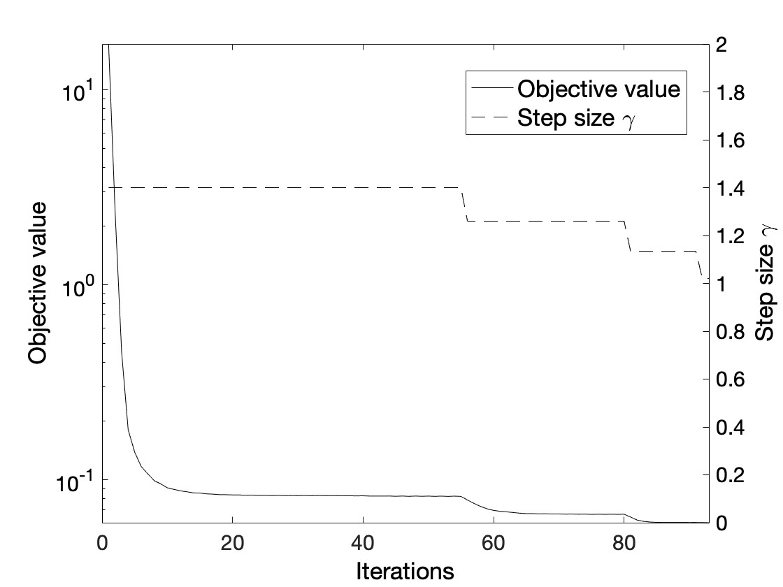
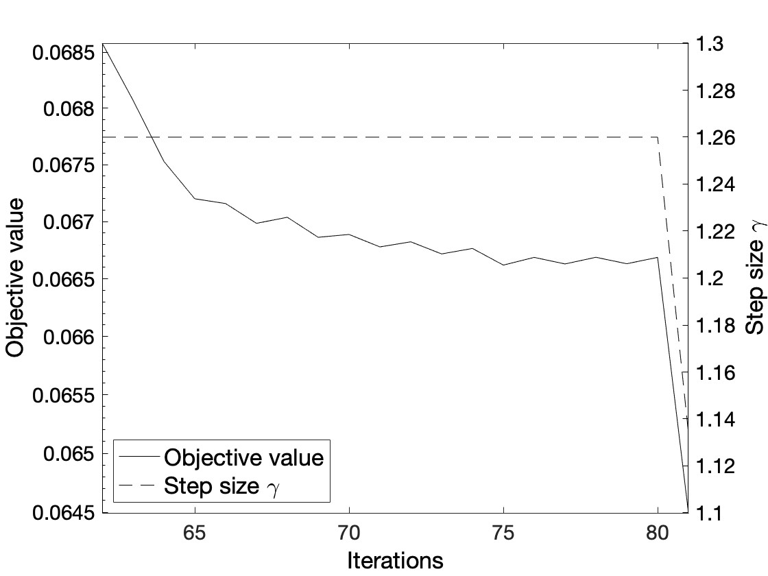
Figure 1. Objective values produced by (PS) with initial value $\gamma=1.4$, $h=\sqrt{2}/50$, $|\mathcal{D}_{k}^{\textup{loc}}|=5000$, and $\bar{s}=0.1$.

The errors from (8.2) as well as the objective value and the computing times for this example for the different data sets $\mathcal{D}_{k}^{\textup{loc}}$, various noise levels $\bar{s}$, and different mesh sizes are shown in Table 3. In addition, the number of iterations and the computing times for the various objectives are listed.

Grid	Data set		Objective value				$\texttt{err}_{L^{2}}$				$\texttt{err}_{H^{1}_{0}}$				Iterations				Time
$N$	$|\mathcal{D}_{k}^{\textup{loc}}|$	$\bar{s}$	(PG)	(PS)	(DR1)	(DR2)	(PG)	(PS)	(DR1)	(DR2)	(PG)	(PS)	(DR1)	(DR2)	(PG)	(PS)	(DR1)	(DR2)	(PG)	(PS)	(DR1)	(DR2)
50	5000	0.1	7.841e-02	6.034e-02	2.155e-01	1.499e-01	5.728e-03	2.199e-03	4.759e-03	2.353e-03	4.075e-02	3.930e-02	4.480e-02	4.215e-02	11	93	76	57	2.488	8.027	12.060	9.741
		0.01	7.617e-02	5.916e-02	1.576e-01	1.377e-01	4.729e-03	2.590e-03	2.388e-03	2.395e-03	3.461e-02	3.337e-02	3.751e-02	3.648e-02	15	86	86	59	2.755	7.571	14.135	10.058
		0.001	7.438e-02	5.814e-02	1.510e-01	1.313e-01	4.542e-03	2.342e-03	2.886e-03	2.164e-03	3.441e-02	3.333e-02	3.783e-02	3.620e-02	10	85	62	60	2.418	7.504	10.407	10.228
		0	7.669e-02	5.857e-02	1.547e-01	1.310e-01	4.799e-03	2.337e-03	3.014e-03	1.979e-03	3.470e-02	3.331e-02	3.808e-02	3.637e-02	11	87	62	61	2.506	7.639	10.413	10.381
50	10000	0.1	5.282e-02	4.429e-02	1.513e-01	9.142e-02	7.521e-03	3.387e-03	2.713e-03	3.493e-03	3.907e-02	3.811e-02	4.158e-02	3.924e-02	16	103	70	53	2.908	9.324	12.276	9.782
		0.01	5.245e-02	4.327e-02	9.670e-02	8.442e-02	3.608e-03	2.297e-03	2.493e-03	1.884e-03	3.322e-02	3.263e-02	3.542e-02	3.420e-02	13	93	62	58	2.693	8.573	11.538	10.891
		0.001	5.228e-02	4.338e-02	9.398e-02	8.446e-02	3.468e-03	2.317e-03	2.791e-03	2.186e-03	3.321e-02	3.252e-02	3.519e-02	3.441e-02	15	75	62	60	2.833	7.300	11.602	11.267
		0	5.332e-02	4.429e-02	9.332e-02	8.526e-02	3.751e-03	2.277e-03	1.385e-03	2.028e-03	3.316e-02	3.256e-02	3.511e-02	3.441e-02	14	123	85	63	2.763	10.712	15.754	11.796
50	50000	0.1	3.310e-02	2.998e-02	8.089e-02	4.559e-02	8.189e-03	2.355e-03	3.023e-03	1.492e-03	3.847e-02	3.792e-02	3.686e-02	3.639e-02	11	78	157	53	3.119	11.476	44.129	15.502
		0.01	3.222e-02	2.966e-02	4.670e-02	3.830e-02	2.407e-03	1.999e-03	2.625e-03	1.948e-03	3.214e-02	3.192e-02	3.292e-02	3.220e-02	11	85	62	58	3.125	12.414	21.290	18.862
		0.001	3.256e-02	2.987e-02	3.976e-02	3.804e-02	2.372e-03	2.048e-03	2.454e-03	1.635e-03	3.210e-02	3.187e-02	3.262e-02	3.230e-02	19	88	62	63	4.075	12.700	21.534	20.895
		0	3.227e-02	2.982e-02	3.933e-02	3.777e-02	2.417e-03	2.118e-03	2.380e-03	1.799e-03	3.210e-02	3.186e-02	3.259e-02	3.210e-02	16	84	62	59	3.807	12.282	21.654	19.565
50	100000	0.1	2.932e-02	2.738e-02	6.180e-02	3.777e-02	9.482e-03	1.854e-03	1.779e-03	1.671e-03	3.837e-02	3.772e-02	3.606e-02	3.578e-02	12	91	170	53	4.223	20.768	77.888	24.637
		0.01	2.983e-02	2.796e-02	4.141e-02	3.263e-02	2.375e-03	2.111e-03	2.168e-03	1.884e-03	3.204e-02	3.184e-02	3.265e-02	3.191e-02	15	92	62	58	4.831	20.908	35.731	31.038
		0.001	2.967e-02	2.802e-02	3.341e-02	3.185e-02	2.388e-03	2.091e-03	2.375e-03	1.234e-03	3.195e-02	3.175e-02	3.235e-02	3.186e-02	24	109	62	83	6.690	24.436	36.423	50.621
		0	2.982e-02	2.794e-02	3.284e-02	3.152e-02	2.311e-03	2.058e-03	2.454e-03	1.598e-03	3.196e-02	3.174e-02	3.232e-02	3.180e-02	16	98	62	59	5.068	22.188	36.668	32.388
100	5000	0.1	5.375e-02	3.622e-02	1.672e-01	1.139e-01	5.097e-03	2.123e-03	2.942e-03	2.211e-03	3.218e-02	2.966e-02	3.365e-02	3.133e-02	16	101	124	60	18.214	44.105	88.854	50.289
		0.01	5.250e-02	3.598e-02	1.327e-01	1.067e-01	4.205e-03	1.835e-03	2.482e-03	1.371e-03	2.192e-02	1.910e-02	2.616e-02	2.369e-02	18	109	151	59	18.748	46.334	108.851	49.967
		0.001	4.894e-02	3.511e-02	1.250e-01	1.022e-01	3.442e-03	1.504e-03	1.872e-03	1.128e-03	2.133e-02	1.900e-02	2.602e-02	2.320e-02	14	98	62	60	17.622	43.469	52.414	50.571
		0	5.105e-02	3.507e-02	1.248e-01	1.051e-01	3.544e-03	1.638e-03	2.017e-03	1.223e-03	2.174e-02	1.894e-02	2.584e-02	2.356e-02	15	95	186	60	17.949	42.387	132.577	50.536
100	10000	0.1	3.336e-02	2.404e-02	1.003e-01	6.893e-02	7.693e-03	2.599e-03	2.138e-03	2.387e-03	3.017e-02	2.796e-02	2.918e-02	2.826e-02	14	96	153	58	17.698	43.270	108.273	49.992
		0.01	3.290e-02	2.324e-02	7.563e-02	6.133e-02	2.586e-03	1.365e-03	1.614e-03	1.124e-03	1.937e-02	1.793e-02	2.261e-02	2.064e-02	13	104	62	59	17.472	45.548	54.508	51.185
		0.001	3.266e-02	2.346e-02	7.415e-02	6.071e-02	2.492e-03	1.275e-03	1.958e-03	1.030e-03	1.926e-02	1.783e-02	2.262e-02	2.053e-02	18	121	62	60	18.898	50.560	54.112	51.783
		0	3.287e-02	2.385e-02	7.463e-02	6.186e-02	2.501e-03	1.477e-03	2.031e-03	1.221e-03	1.924e-02	1.790e-02	2.255e-02	2.057e-02	17	109	62	60	18.582	47.091	54.112	51.816
100	50000	0.1	1.521e-02	1.228e-02	3.220e-02	2.723e-02	8.192e-03	1.810e-03	8.163e-04	1.543e-03	2.846e-02	2.758e-02	2.466e-02	2.517e-02	16	100	332	53	19.213	49.814	251.952	52.959
		0.01	1.403e-02	1.157e-02	2.808e-02	2.008e-02	1.575e-03	1.216e-03	6.625e-04	9.816e-04	1.720e-02	1.672e-02	1.855e-02	1.728e-02	22	110	85	59	21.289	53.372	89.297	60.222
		0.001	1.425e-02	1.156e-02	2.165e-02	1.971e-02	1.595e-03	1.252e-03	1.629e-03	9.382e-04	1.714e-02	1.659e-02	1.812e-02	1.711e-02	17	114	62	103	19.565	54.822	68.245	103.937
		0	1.412e-02	1.157e-02	2.103e-02	1.945e-02	1.524e-03	1.259e-03	1.587e-03	4.632e-04	1.707e-02	1.661e-02	1.803e-02	1.708e-02	23	134	62	111	21.630	61.853	68.280	113.192
100	100000	0.1	1.183e-02	9.950e-03	2.087e-02	1.870e-02	1.002e-02	1.104e-03	7.591e-04	7.054e-04	2.840e-02	2.710e-02	2.393e-02	2.360e-02	15	136	295	163	20.175	74.482	276.409	157.545
		0.01	1.157e-02	9.637e-03	2.180e-02	1.416e-02	1.543e-03	1.246e-03	5.781e-04	8.339e-04	1.693e-02	1.648e-02	1.787e-02	1.669e-02	23	156	85	59	23.568	83.122	116.541	73.134
		0.001	1.147e-02	9.631e-03	1.470e-02	1.335e-02	1.572e-03	1.252e-03	1.640e-03	9.232e-04	1.681e-02	1.636e-02	1.749e-02	1.657e-02	36	141	62	60	29.353	76.426	88.675	76.115
		0	1.146e-02	9.607e-03	1.443e-02	1.317e-02	1.505e-03	1.262e-03	1.614e-03	3.616e-04	1.680e-02	1.637e-02	1.743e-02	1.652e-02	18	197	62	114	21.525	100.915	88.232	156.888
200	5000	0.1	4.101e-02	2.840e-02	1.347e-01	1.006e-01	5.324e-03	2.168e-03	1.941e-03	1.975e-03	3.083e-02	2.772e-02	2.977e-02	2.851e-02	17	93	211	61	249.322	370.015	813.302	411.318
		0.01	4.000e-02	2.778e-02	1.166e-01	9.346e-02	3.989e-03	1.582e-03	1.083e-03	1.073e-03	1.740e-02	1.347e-02	2.107e-02	1.888e-02	25	115	236	61	260.467	398.098	898.825	411.689
		0.001	3.730e-02	2.679e-02	1.084e-01	8.936e-02	3.152e-03	1.284e-03	7.409e-04	1.035e-03	1.663e-02	1.316e-02	2.055e-02	1.839e-02	31	92	290	59	268.484	368.304	1056.849	406.249
		0	3.893e-02	2.699e-02	1.092e-01	9.197e-02	3.340e-03	1.398e-03	7.797e-04	1.119e-03	1.703e-02	1.321e-02	2.102e-02	1.875e-02	19	100	305	61	253.189	378.503	1102.067	412.168
200	10000	0.1	2.442e-02	1.706e-02	7.392e-02	5.868e-02	7.643e-03	2.432e-03	1.449e-03	2.013e-03	2.885e-02	2.586e-02	2.552e-02	2.506e-02	18	110	214	60	252.154	393.617	826.667	411.387
		0.01	2.402e-02	1.661e-02	6.925e-02	5.209e-02	2.346e-03	1.212e-03	1.586e-03	9.581e-04	1.405e-02	1.159e-02	1.817e-02	1.509e-02	20	106	62	60	254.167	389.364	421.967	412.413
		0.001	2.377e-02	1.669e-02	6.744e-02	5.215e-02	2.202e-03	1.165e-03	1.644e-03	9.331e-04	1.378e-02	1.145e-02	1.792e-02	1.492e-02	21	117	62	60	256.723	401.675	422.083	411.567
		0	2.432e-02	1.695e-02	6.787e-02	5.222e-02	2.446e-03	1.213e-03	1.835e-03	9.034e-04	1.389e-02	1.147e-02	1.802e-02	1.505e-02	22	99	62	61	256.975	378.268	421.892	416.442
200	50000	0.1	1.007e-02	7.268e-03	2.080e-02	1.968e-02	8.088e-03	1.794e-03	6.689e-04	7.355e-04	2.662e-02	2.547e-02	2.155e-02	2.141e-02	19	130	208	197	254.379	434.248	840.326	800.123
		0.01	9.390e-03	6.664e-03	2.213e-02	1.485e-02	1.352e-03	1.055e-03	9.224e-04	7.493e-04	1.071e-02	9.705e-03	1.222e-02	1.058e-02	26	155	153	60	263.740	492.920	750.784	423.843
		0.001	9.451e-03	6.711e-03	1.664e-02	1.416e-02	1.302e-03	1.079e-03	1.514e-03	4.517e-04	1.046e-02	9.488e-03	1.204e-02	1.009e-02	28	142	62	150	267.072	471.474	450.813	727.345
		0	9.415e-03	6.645e-03	1.628e-02	1.396e-02	1.315e-03	1.065e-03	1.461e-03	1.922e-04	1.045e-02	9.486e-03	1.195e-02	1.007e-02	22	142	62	177	258.197	447.639	451.086	834.282
200	100000	0.1	7.182e-03	5.326e-03	1.227e-02	1.153e-02	1.013e-02	9.817e-04	6.327e-04	5.901e-04	2.637e-02	2.489e-02	2.084e-02	2.067e-02	18	124	348	381	254.638	435.492	1296.349	1379.963
		0.01	6.984e-03	5.091e-03	1.594e-02	9.382e-03	1.393e-03	1.089e-03	9.057e-04	6.660e-04	1.013e-02	9.352e-03	1.133e-02	9.655e-03	49	207	153	59	300.392	558.922	839.098	437.614
		0.001	6.943e-03	5.030e-03	1.013e-02	8.310e-03	1.382e-03	1.101e-03	1.503e-03	3.327e-04	9.893e-03	9.096e-03	1.104e-02	9.155e-03	38	234	62	154	283.820	598.549	487.794	824.306
		0	6.963e-03	5.004e-03	9.859e-03	8.093e-03	1.374e-03	1.084e-03	1.467e-03	1.343e-04	9.906e-03	9.078e-03	1.099e-02	9.108e-03	37	178	62	181	282.477	512.666	487.917	967.058

Table 3. Non-linear law tested on $\Omega=(0,1)^{2}$ with different mesh sizes and data sets.

The following observations can be made:

With respect to accuracy, all algorithms deliver comparable results with (PS) being slightly superior regarding the objective and $\texttt{err}_{H^{1}_{0}}$ and (DR2) being slightly superior regarding $\texttt{err}_{L^{2}}$. To see this more clearly, we highlight the largest differences (compared to the result of (PS) and (DR2), respectively) concerning objective value and the errors $\texttt{err}_{L^{2}}$ and $\texttt{err}_{H^{1}_{0}}$ in boldface.

With regard to the effort, the simple projection method (PG) is nearly always the best. This concerns the number of iterations as well as the consumed computing time. Moreover, the differences are substantial. For instance, in the line highlighted in boldface, (PG) is up to approximately 5, 18, and 8 times faster than (PS), (DR1), and (DR2), respectively.

In accordance with our theoretical findings, the objective value decreases if the noise level $\bar{s}$ is reduced and/or if the data sample set is getting larger. Concerning the noise level, this reduction is however rather moderate. Even the largest reduction indicated with gray background is by less than 10 %, though $\bar{s}$ is reduced from 0.1 to zero. Regarding the errors $\texttt{err}_{L^{2}}$ and $\texttt{err}_{H^{1}_{0}}$, the dependency on the noise level is indifferent. The largest reduction, again indicated by gray background, is about 80 % w.r.t. the $L^{2}$-error and 65 % for the $H^{1}_{0}$-error. On the other hand, there are also instances, two of them marked in light gray, where the errors not only stagnate, but even increase with decreasing noise. In summary, the influence of the noise level appears to be limited and all algorithms behave comparatively robust w.r.t. noisy data.

The situation changes when the sample size is changed. With respect to the sample size, the reduction of the objective is more significant. Here, the largest reduction, when increasing the sample size from 5.000 to 10.000, marked by a box, is about 80 %. In case of the $L^{2}$-error, the largest reduction is about one order of magnitude, while the largest reduction of $\texttt{err}_{H^{1}_{0}}$ is approximately 35 %, both again marked by boxes. In summary, the sample size has a significantly larger impact on the accuracy of the results than the noise level.

The influence of the mesh size to the $L^{2}$- and the $H^{1}_{0}$-error is similar to that of “classical” finite element simulations. We highlight the smallest $L^{2}$- and $H^{1}_{0}$-error for zero noise level and maximum $|\mathcal{D}_{k}^{\textup{loc}}|$ in italic type. In case of $\texttt{err}_{L^{2}}$, the best result is obtained by (DR2), in case of $\texttt{err}_{H^{1}_{0}}$ by (PS). In Table 4, these values are compared with a “classical” finite element computation. For the latter, we discretized (1.1) with $\kappa$ as defined in (8.3) by choosing $U_{h}$ from (8.1) as trial and test space. The resulting nonlinear system of equation is solved by Newton’s method. The relative errors are denoted by $\texttt{err}_{L^{2}}^{\textup{FE}}$ and $\texttt{err}_{H^{1}_{0}}^{\textup{FE}}$, respectively. We moreover present the experimental order of convergence defined by

$$\texttt{EOC}_{L^{2}}^{\textup{FE}}:=\frac{\log(\texttt{err}_{L^{2}}^{\textup{FE}}(h_{1}))-\log(\texttt{err}_{L^{2}}^{\textup{FE}}(h_{2}))}{\log(h_{1})-\log(h_{2})},$$

where $h_{1}$ and $h_{2}$ are two mesh sizes and $\texttt{err}_{L^{2}}^{\textup{FE}}(h_{i})$, $i=1,2$, the associated relative $L^{2}$-errors. Furthermore, $\texttt{EOC}_{H^{1}_{0}}^{\textup{FE}}$ is defined analogously and $\texttt{EOC}_{L^{2}}^{\textup{DR2}}$ and $\texttt{EOC}_{H^{1}_{0}}^{\textup{PS}}$ denote the respective orders of convergence generated by the data driven approach with (DR2) and (PS), respectively.

N	$\texttt{err}_{L^{2}}^{\textup{FE}}$	$\texttt{EOC}_{L^{2}}^{\textup{FE}}$	$\texttt{err}_{L^{2}}^{\textup{DR2}}$	$\texttt{EOC}_{L^{2}}^{\textup{DR2}}$	$\texttt{err}_{H^{1}_{0}}^{\textup{FE}}$	$\texttt{EOC}_{H^{1}_{0}}^{\textup{FE}}$	$\texttt{err}_{H^{1}_{0}}^{\textup{PS}}$	$\texttt{EOC}_{H^{1}_{0}}^{\textup{PS}}$
50	1.601e-03	—	1.598e-03	—	3.143e-02	—	3.174e-02	—
100	4.004e-04	1.9995	3.616e-04	2.1438	1.571e-02	1.0005	1.637e-02	0.9552
200	1.001e-04	2.0000	1.343e-04	1.4289	7.854e-03	1.0002	9.078e-03	0.8506

Table 4. Relative errors and experimental orders of convergence for the “classical” finite element solution and the best results of the data-driven approach in dependence of the mesh sizes $h=\frac{\sqrt{2}}{N}$.

As the theory predicts, cf. e.g. [5], Table 4 shows a quadratic and a linear order of convergence for the relative errors $\texttt{err}_{L^{2}}^{\textup{FE}}$ and $\texttt{err}_{H^{1}_{0}}^{\textup{FE}}$, respectively. We moreover observe that the errors produced by the data driven approach are more or less of the same size as the “classical” finite element error except for the smallest mesh with $N=200$, where the error caused by the sample size becomes predominant compared to the error induced by the mesh.

To summarize, it is to be noted that the accuracy of all algorithms improve, if the noise level is reduced, the data sample set is enlarged, and the mesh is refined, with the noise level having the smallest impact on the accuracy. We moreover observe that all algorithms yield satisfactorily results w.r.t. the accuracy, the best results being even comparable to a “classical” finite element computation. Concerning the performance of the algorithms, the original projection algorithm (PG) turns out to be superior in the sense that it provides an accuracy similar to the other algorithms with the fastest computing time. The proximal gradient method defined by (PS) in average returns the most accurate results (in particular w.r.t. the $H^{1}_{0}$-seminorm) but with a greater computational effort. Both variants of the Douglas-Rachford algorithm also provide comparable results but one has to be cautious concerning the termination criterion due to the lack of fixed points.

9. Conclusion and Outlook

In this paper, we studied a finite element discretization of the data driven approach as introduced [19], where we focused on a stationary scalar diffusion problem. We showed that the finite element error analysis can be incorporated into the data convergence analysis of [10] as long as finite elements are used where a vanishing discretized divergence implies that the continuous divergence vanishes, too, cf. Lemma 3.3(i). In the conductivity example, i.e., our stationary scalar diffusion problem, the construction of such elements is comparatively simple and, for instance, Raviart-Thomas elements do the job, see Proposition 3.7. The situation changes, if one turns to problems in elasticity, where the symmetry of the stress tensor significantly complicates the construction of such elements, see for instance [4, Section 4] and [2]. The considerations in Section 6 however indicate that the use of “classical” piecewise linear and continuous finite elements might not be feasible in context of the data driven approach, an aspect that gives rise to future research. Nevertheless, if $H(\operatorname{div})$-conforming finite elements fulfilling Assumptions 3.1 are used, then, under suitable assumptions on the approximation of the local data set, see (5.7), we obtain the same approximation results as in [10] so that (subsequences of) minimizers of the finite dimensional problems (P_k) converge in data to elements of the intersection $\overline{\mathcal{D}}\cap\mathcal{E}$.

Another issue concerns the computation of minimizers of (P_k). As seen in Section 7.2, the discretized data driven problem (P_k) is equivalent to a quadratic semi-assignment problem and, as such, NP-hard, see Remark 7.1. There is thus no hope to find an efficient algorithm for the computation of minimizers. We therefore presented two heuristic approaches, one based on projections on $\mathcal{E}_{h}$ and $\mathcal{D}_{h}$, the other one based on a local search in combination with model order reduction. It turns out that, the local search is not competitive, at least for the example of Fourier’s law. There are however plenty of parameters to adjust, such as the size of the POD basis and the neighborhood within the local search, and it requires further investigations to analyze if a smart choice of the parameters could result in a competitive algorithm. With regard to the projection-type methods, the most simple alternating projection algorithm according to [19] turns out to be advantageous with respect to the ratio of accuracy and computational time. With regard to accuracy only, the modified projection method (PS) and a variant of the Douglas-Rachford algorithm delivered the best results. If the noise level is zero and the sample size is large enough, then these results are comparable to a “classical” finite element simulation with known material law. There is however no theoretical evidence for a convergence of the projection-based methods, even not to any kind of fixed-point, not to mention a minimizer of (P_k), and the examples in [18] show that this is indeed an issue. The robustification of projection-based methods for a reliable solution of (P_k) is probably one of the most important open problems in the context of data driven numerics.

References

- [1] F. J. Aragón Artacho, R. Campoy, and M. K. Tam. The douglas–rachford algorithm for convex and nonconvex feasibility problems. Mathematical Methods of Operations Research, 91(2), 2020.
- [2] D.N. Arnold, F. Brezzi, and J. Douglas. PEERS: A new mixed finite element for plane elasticity. Japan J. Appl. Math., 1:347–367, 1984.
- [3] A. Beck. First-Order Methods in Optimization. Society for Industrial and Applied Mathematics, Philadelphia, PA, 2017.
- [4] D. Braess. Finite Elements: Theory, Fast Solvers, and Applications in Solid Mechanics. Cambridge University, 3. edition, 2007.
- [5] C.S. Brenner and R.L. Scott. The Mathematical Theory of Finite Element Methods. Springer-Verlag, New York, 1994.
- [6] C. Buchheim and E. Traversi. Quadratic combinatorial optimization using separable underestimators. INFROMS Journal on Computing, 30(3):424–437, 2018.
- [7] P. Carrara, L. De Lorenzis, L. Stainier, and M. Ortiz. Data-driven fracture mechanics. Computer Methods in Applied Mechanics and Engineering, 372:113390, 2020.
- [8] C. Clason and T. Valkonen. Introduction to nonsmooth analysis and optimization, 2020.
- [9] S. Conti, S. Müller, and M. Ortiz. Data-driven problems in elasticity. Archive for Rational Mechanics and Analysis, 229(1):79–123, Jan 2018.
- [10] S. Conti, S. Müller, and M. Ortiz. Data-driven finite elasticity. Archive for Rational Mechanics and Analysis, 237(1):1–33, 2020.
- [11] R. G. Durán. Mixed finite element methods. In Mixed Finite Elements, Compatibility Conditions, and Applications: Lectures given at the C.I.M.E. Summer School held in Cetraro, Italy June 26–July 1, 2006, pages 1–44. Springer Berlin Heidelberg, 2008.
- [12] R. Eggersmann, T. Kirchdoerfer, S. Reese, L. Stainier, and M. Ortiz. Model-free data-driven inelasticity. Computer Methods in Applied Mechanics and Engineering, 350:81–99, 2019.
- [13] R. Eggersmann, L. Stainier, M. Ortiz, and S. Reese. Model-free data-driven computational mechanics enhanced by tensor voting. Computer Methods in Applied Mechanics and Engineering, 373:113499, 2021.
- [14] Jerome H. Friedman, Jon Louis Bentley, and Raphael Ari Finkel. An algorithm for finding best matches in logarithmic expected time. 3(3), 1977.
- [15] Martin Kahlbacher and Stefan Volkwein. Galerkin proper orthogonal decomposition methods for parameter dependent elliptic systems. Discussiones Mathematicae, Differential Inclusions, Control and Optimization, 27(1):95–117, 2007.
- [16] Y. Kanno. Data-driven computing in elasticity via kernel regression. Theoretical and Applied Mechanics Letters, 8:361–365, Dec 2018.
- [17] Y. Kanno. Simple heuristic for data-driven computational elasticity with material data involving noise and outliers: a local robust regression approach. Japan Journal of Industrial and Applied Mathematics, 3(1085–1101), 2018.
- [18] Y. Kanno. Mixed-integer programming formulation of a data-driven solver in computational elasticity. Optimization Letters, 13(7):1505–1514, 2019.
- [19] T. Kirchdoerfer and M. Ortiz. Data-driven computational mechanics. Computer Methods in Applied Mechanics and Engineering, 304:81–101, 2016.
- [20] T. Kirchdoerfer and M. Ortiz. Data-driven computing in dynamics. International Journal for Numerical Methods in Engineering, 113, Jun 2017.
- [21] C. Natemeyer and D. Wachsmuth. A proximal gradient method for control problems with non-smooth and non-convex control cost. Computational Optimization and Applications, 80(2):639–677, 2021.
- [22] L.T.K. Nguyen and M.-A. Kneip. A data-driven approach to nonlinear elasticity. Computers & Structures, 194:97–115, 2018.
- [23] K. Poelstra, T. Bartel, and B. Schweizer. A data driven framework for evolutionary problems in solid mechanics. No. 2021-02, Preprints der Fakultät für Mathematik, TU Dortmund, 2021.
- [24] M. Röger and B. Schweizer. Relaxation analysis in a data driven problem with a single outlier. Calc. Var., 59(119), 2020.
- [25] S. Sahni and T. Gonzalez. P-complete approximation problems. Journal of the ACM (JACM), 23(3):555–565, 1976.
- [26] R. Temam. Navier-Stokes Equations. North-Holland, Amsterdam, New-York, Oxford, 1977.
- [27] Sebastian Ullmann, Marko Rotkvic, and Jens Lang. Pod-galerkin reduced-order modeling with adaptive finite element snapshots. Journal of Computational Physics, 325:244–258, 2016.
- [28] D. Wachsmuth. Iterative hard-thresholding applied to optimal control problems with control cost. SIAM J. Control Optim., 57(2):854–879, 2019.