Cramér-Rao Bounds for Near-Field Sensing
with Extremely Large-Scale MIMO

Abstract

Mobile communication networks were designed to mainly support ubiquitous wireless communications, yet they are also expected to achieve radio sensing capabilities in the near future. However, most prior studies on radio sensing usually rely on far-field assumption with uniform plane wave (UPW) models. With the ever-increasing antenna size, together with the growing demands to sense nearby targets, the conventional far-field UPW assumption may become invalid. Therefore, this paper studies near-field radio sensing with extremely large-scale (XL) antenna arrays, where the more general uniform spheric wave (USW) sensing model is considered. Closed-form expressions of the Cramér-Rao Bounds (CRBs) for both angle and range estimations are derived for near-field XL-MIMO radar mode and XL-phased array radar mode, respectively. Our results reveal that different from the conventional UPW model where the CRB for angle decreases unboundedly as the number of antennas increases, for XL-MIMO radar-based near-field sensing, the CRB decreases with diminishing return and approaches to a certain limit as the number of antennas increases. Besides, different from the far-field model where the CRB for range is infinity since it has no range estimation capability, that for the near-field case is finite. Furthermore, it is revealed that the commonly used spherical wave model based on second-order Taylor approximation is insufficient for near-field CRB analysis. Extensive simulation results are provided to validate our derived CRBs.

I introduction

With the fifth-generation (5G) mobile communication networks being commercially deployed, researchers have started the investigation of the key technologies for the sixth-generation (6G) networks [2, 3, 4]. There is no doubt that 6G will continue to significantly improve the performance of wireless communications, in terms of coverage, connectivity density, data rate, latency, etc. On the other hand, it is also widely believed that 6G should go beyond communications, by providing various new services such as high-performance ubiquitous localization and radar sensing [5, 6, 7], which is possible thanks to the continuous expansion of cellular bandwidth and the ever-increasing of antenna size. Therefore, the integration of sensing and communication has received significant research interest recently, under various terms like joint communication and radar/radio sensing (JCAS) [8], dual-functional radar communications (DFRC) [9], and integrated sensing and communication (ISAC) [10].

Most of the research on ISAC can be loosely categorized into waveform design[11, 12, 13, 14, 15], codebook design[16], beam alignment  [17][18] and information-theoretical limits analysis[19, 20, 21], etc. For radar sensing, several estimation-theoretic metrics such as Cramér-Rao Bound (CRB)[22], Weiss-Wdinstein Bound [23] and Ziv-Zakai Bound [24] are used to evaluate the performance of parameter estimations, such as propagation delay, angle of arrival/departure (AoA/AoD), Doppler frequency, etc. Perhaps the most commonly used bound for parameter estimation is CRB, which serves as a lower bound for unbiased mean-square error (MSE) estimator. Different CRBs have been derived for two typical radar sensing modes, namely MIMO radar mode and phased array radar mode[25]. For MIMO radar mode, orthogonal waveforms are transmitted from different antennas, so as to obtain the waveform diversity gain. In this case, both colocated and distributed MIMO radar systems have been studied in terms of CRB analysis[26, 27, 28]. On the other hand, for phased array radar mode, coherent waveforms are transmitted from different antennas, so as to obtain high transmit coherent processing gain. The CRBs for monostatic phased array radar system with single transmit antenna and muti-antenna arrays have been studied in [29] and [30], respectively. Existing results in [26] reveal that for both MIMO and phased array radar modes, the CRBs for angle estimation decrease indefinitely with the increase of signal-to-noise ratios (SNRs) and the number of transmit and receive antennas.

On the other hand, MIMO communications have been tremendously advanced from small MIMO in 4G to massive MIMO in 5G[31]. Looking forward towards 6G, there have been growing interests in the study of extremely large-scale MIMO (XL-MIMO)[32, 33, 34, 35, 36], for which the antenna size is so large that conventional far-field assumption with uniform plane wave (UPW) models become invalid. Instead, the more generic spherical wavefront characteristics need to be taken into account[1]. However, most existing studies mentioned above for CRB analysis mainly rely on the conventional UPW models[37], which was justifiable since most prior radar sensing applications were mainly for distant targets and the antenna size is usually moderate. With the ever-increasing antenna size at base stations (BSs), together with the growing demands to also sense nearby targets, it is necessary to develop new CRB analysis for near-field sensing, without restricting to the conventional far-field UPW models.

There are some relevant works for CRB analysis that consider the near field effect for source localization problems[38, 39, 40, 41]. For example, Fresnel approximation based on second-order Taylor approximation is commonly used to approximate spherical wavefront[38][39]. In [42], a near-field tracking problem for inferring the position and velocity of a moving source was considered, and the posterior Cramér-Rao Lower Bound was derived. However, although such a second-order Taylor approximation method well fits the exact near-field uniform spheric wave (USW) model in most practical systems, it may introduce some systematic errors and make the model asymptotically biased[43]. Moreover, most existing results are derived for the source localization problem that involves only one-hop signal propagation, which cannot be applied for radar sensing scenario with double-hop signal propagation. In [40], the authors derived the conditional and unconditional CRBs for near-field bistatic MIMO radar system. However, such results were dependent on the derivative of the path difference with respect to unknown parameters, which is difficult to gain insights between the CRBs and the key system parameters or array configuration. To the best of our knowledge, closed-form CRB expressions in terms of the key system parameters, such as SNR and number of antennas, have not been reported for near-field radar sensing taking into account uniform spherical wave (USW) characteristics. This motivates our current work. The main contributions of this paper are summarized as follows:

• First, we present the near-field bistatic sensing model with extremely large-scale antenna arrays, for which the signal processing procedures for XL-MIMO radar mode and XL-phased array radar mode are introduced, respectively. It is found that directly deriving the CRBs for near-field bistatic sensing is challenging, since it involves four-dimension parameter estimation, including transmitter-side and receiver-side angles and ranges, respectively. To tackle this difficulty, we transform the problem into two-dimensional parameter estimation problem by exploiting the geometrical relationship between the transmit and receive arrays, so that the receiver-side parameters can be represented in terms of the transmitter-side parameters.

• Next, to gain useful insights, the basic monostatic near-field sensing is first considered, which can be viewed as a special case of the general bistatic near-field sensing. The closed-form expressions of the near-field CRBs for angle and range estimation are derived. The asymptotic cases with very large target range or antenna size are respectively considered to gain useful insights. It is revealed that our newly derived CRBs for near-field USW-based sensing include the results based on the conventional far-field UPW model as special cases. Different from the conventional far-field sensing, for XL-MIMO near-field sensing, the CRB for angle estimation no longer decreases indefinitely as the array size increases. Instead, it would approach to a limit that is dependent on the inter-element spacing. Moreover, the CRB for range estimation, which is infinity in conventional UPW model, is shown to be finite in the near-field case, showing the capability for range discrimination with XL-MIMO near-field sensing.

• Finally, for the more general bistatic XL-MIMO sensing, as it is quite challenging to derive the closed-form CRB expressions when near-field USW model is considered at both transmitter and receiver sides, we consider the more tractable and likely scenario in practice that the sensing target locates in the near-field of the transmit array. The corresponding closed-form CRBs of angle and range are derived and useful insights are obtained. Furthermore, by comparing our CRBs with the classic Capon algorithm [44], numerical results are provided to validate our derived near-field CRBs.

The rest of this paper is organized as follows. Section II introduces the general near-field USW model for bistatic radar sensing, together with the key radar signal processing procedures for XL-MIMO radar mode and XL-phased array radar mode, respectively. Section III derives the closed-form expression of CRB for the monostatic scenario, which can be treated as a special case of bistatic sensing. Section IV derives the CRBs for bistatic sensing when the sensing target is located at the near field of the transmit array. Section V provides numerical results to validate our derived CRBs.

Notations: Lower and upper-case bold letters denote vectors and matrices, respectively. ${\bf{z}}_{i}$ denotes the $i$-th element of a vector ${\bf z}$. ${\bf{Z}}^{T}$, ${\bf{Z}}^{*}$, ${\bf{Z}}^{H}$ and$\ \det({\bf{Z}})\$denote the transpose, conjugate, conjugate transpose, and determinant of the matrix ${\bf{Z}}$, respectively. $\mathcal{R\{\cdot\}}$ denotes the real part, and$\ \otimes\$denotes the Kronecker product.$\ \frac{\partial}{{\partial z}}\left(\cdot\right)\$denotes the partial derivative of $z$.$\ {{\bf{1}}_{L}}\$denotes the vector of dimension$\ L\times 1\$with all ones. Finally, $j$ denotes the imaginary unit and$\ {\|{\bf{z}}\|}$ denotes the Euclidean norm of vector $\ {\bf{z}}\$.

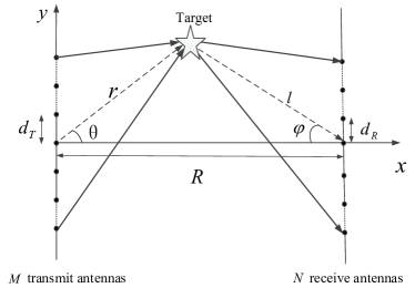
Figure 1: Near-field radar sensing with XL-MIMO.

II System model

As shown in Fig.1, we consider a near-field radar sensing system with XL-MIMO. Let $M\gg 1$ and $N\gg 1$ denote the number of transmit and receive antenna elements, respectively. For notational convenience, we assume that $M$ and $N$ are odd numbers. Furthermore, both the transmitter and receiver are equipped with uniform linear arrays (ULAs) with inter-element spacing denoted by $d_{T}$ and $d_{R}$, respectively. Thus, the array apertures of the transmitter and receiver are$\ {D_{T}}\approx M{d_{T}}\$and$\ {D_{R}}\approx N{d_{R}},\$respectively. For simplicity, we assume that the transmit and receive ULAs are parallel to each other and their distance is $R$. Without loss of generality, the transmit ULA is placed along the $y$-axis and centered at the origin. Therefore, the location of the $m$th transmit element is$\ {{\bf{w}}_{m}}={[0,m{d_{T}}]^{T}},\$where$\ m\in\mathcal{M}$, with $\mathcal{M}\triangleq\left\{{0,\pm 1,\cdots,\pm{{(M-1)}\mathord{\left/{\vphantom{{(M-1)}2}}\right.\kern-1.2pt}2}}\right\}.\$Similarly, the location of the $n$th receive element is $[R,n{d_{R}}]^{T},\$where$\ n\in\mathcal{N}$, with $\mathcal{N}\triangleq\left\{{0,\pm 1,\cdots,\pm{{(N-1)}\mathord{\left/{\vphantom{{(N-1)}2}}\right.\kern-1.2pt}2}}\right\}.\$Let$\ {\bf{q}}={[r\cos\theta,r\sin\theta]^{T}}\$denotes the location of the radar sensing target, where $r$ is the distance between the target and the center of the transmit array, and$\ \theta\in\left[-\frac{\pi}{2},\frac{\pi}{2}\right]\$is the direction of the target with respect to the normal vector of the transmit array. Therefore, the distance between the target and the $m$th transmit antenna is

$${r_{m}}=\|{{{\bf{w}}_{m}}{\rm{-}}{\bf{q}}}\| =r\sqrt{1-2m{\varepsilon_{T}}\sin\theta+{m^{2}}{\varepsilon_{T}}^{2}},$$ (1)

where$\ {\varepsilon_{T}}\triangleq\frac{{{d_{T}}}}{r}\ll 1.\$Note that (1) is the exact distance expression that can be degenerated to the conventional far-field UPW model by using first-order Taylor approximation when $D_{T}\ll r$.

For XL-MIMO systems, when the far-field assumption no longer holds, the exact distance expression (1) is usually needed to accurately model the signal phase and amplitude variations across different array elements. In this case, the element of the transmit array response vector not only depends on the direction $\theta$, but also on the range $r$, which can be expressed as$\ {\tilde{a}_{m}}(r,\theta)=\frac{{\sqrt{{\alpha_{0}}}}}{{{r_{m}}}}{e^{-j\frac{{2\pi}}{\lambda}{r_{m}}}}$[32], $m\in\mathcal{M}$, with$\ {{\alpha_{0}}}\$denoting the channel power gain at the reference distance of $1$m.

Similarly, let $l$ denotes the distance between the target and the center of the receive antenna array, and $\varphi$ denotes the direction of the target with respect to the normal vector of the receive array. Therefore, the element of the receive array response vector can be expressed as $\ {\tilde{b}_{n}}(l,\varphi)=\frac{{\sqrt{{\beta_{0}}}}}{{{l_{n}}}}{e^{-j\frac{{2\pi}}{\lambda}{l_{n}}}},n\in\mathcal{N},$ with$\ {l_{n}}=l\sqrt{1-2n{\varepsilon_{R}}\sin\varphi+{n^{2}}{\varepsilon_{R}}^{2}}\$denoting the distance between the target and the center of the receive array.$\ {\varepsilon_{R}}\buildrel\Delta\over{=}\frac{{{d_{R}}}}{l}\ll 1,\$and$\ {{\beta_{0}}}\$denotes the channel power gain at the reference distance of $1$m. Furthermore, when the distance $R$ between the transmit and receive arrays is known, the receiver side range and angle parameters $l$ and $\varphi$ can be expressed in terms of the transmitter side parameters $r$ and $\theta$, i.e.,

$$\footnotesize\ \begin{aligned} &l({r,\theta})=\sqrt{{R^{2}}+{r^{2}}-2Rr\cos\theta},\\ &\varphi(r,\theta)=\arcsin\left\{{\frac{{r\sin\theta}}{{\sqrt{{R^{2}}+{r^{2}}-2Rr\cos\theta}}}}\right\}.\ \end{aligned}\$$ (2)

As a result, the distance $l_{n}$ and the element of the receive array response vector ${\tilde{b}_{n}}(l,\varphi)$ can be represented in terms of $r$ and $\theta$ as

$$\footnotesize\ \begin{aligned} \ {l_{n}}({r,\theta})&=\sqrt{{R^{2}}+{r^{2}}-2Rr\cos\theta-2n{d_{R}}r\sin\theta+{n^{2}}{d_{R}}^{2}},\\ \ {\tilde{b}_{n}}(r,\theta)&=\frac{{\sqrt{{\beta_{0}}}}}{{{l_{n}}(r,\theta)}}{e^{-j\frac{{2\pi}}{\lambda}{l_{n}}(r,\theta)}}.\end{aligned}\$$ (3)

Let $x_{m}(t)$ denotes the transmitted waveform by the $m$th transmit antenna, $m\in\mathcal{M}$. The received signal by the $n$th receive antenna due to target reflection can be expressed as

$$\ {r_{n}}(t)=\tilde{\kappa}{\tilde{b}_{n}}(r,\theta)\sum\nolimits_{m=-\frac{{M-1}}{2}}^{\frac{{M-1}}{2}}{{\tilde{a}_{m}}(r,\theta){x_{m}}(t-{\tau})+{n_{n}}(t)},$$ (4)

where $\tilde{\kappa}$ is a complex reflection coefficient that includes the impact of radar cross section (RCS) of the target, $\tau$ is the propagation delay of the reflected signal by the target. Note that we assume that the propagation delays between different transmit and receive elements are approximately equal, which is valid when $D_{T}+D_{R}\leq\frac{c}{B},\$where $B$ denotes system bandwidth, and $c$ is the speed of light. $n_{n}(t)$ is the independent and identically distributed (i.i.d.) additive white Gaussian noise (AWGN) with power spectral density $N_{0}$.

Note that$\ {\tilde{a}_{m}}(r,\theta)\$can be equivalently written as$\ {\tilde{a}_{m}}(r,\theta)=\frac{{\sqrt{{\alpha_{0}}}}}{r}\frac{r}{{{r_{m}}}}{e^{-j\frac{{2\pi}}{\lambda}{r_{m}}}},\$and when $r>1.2D_{T}$[45], the amplitude variations across array elements can be neglected. Therefore, the transmit array response vector can be expressed as ${\tilde{\bf a}}(r,\theta)=\frac{{\sqrt{{\alpha_{0}}}}}{r}{\bf{a}}(r,\theta),$ where

$${\bf{a}}(r,\theta)=[{a_{-\frac{{M-1}}{2}}}(r,\theta),...,{a_{m}}(r,\theta),...,{a_{\frac{{M-1}}{2}}}(r,\theta)]^{T},$$ (5)

with the element$\ {a_{m}}(r,\theta)={e^{-j\frac{{2\pi}}{\lambda}{r_{m}}}}.\$Similarly, the receive response vector can be expressed as ${\tilde{\bf b}}(r,\theta)=\frac{{\sqrt{{\beta_{0}}}}}{l}{\bf{b}}(r,\theta),$ where

$${\bf{b}}(r,\theta)=[{b_{-\frac{{N-1}}{2}}}(r,\theta),...,{b_{n}}(r,\theta),...,{b_{\frac{{N-1}}{2}}}(r,\theta)]^{T},$$ (6)

with$\ {b_{n}}(r,\theta)={e^{-j\frac{{2\pi}}{\lambda}{l_{n}}}}.\$Note that we have expressed the receive array response vector in terms of the transmitter side angle and range parameters $(r,\theta)$ based on the relationship (3). Therefore, according to (4), the vector form of the received signal for bistatic near-field radar sensing can be written as

$$\ {\bf{r}}(t)=\kappa{\bf{b}}(r,\theta){{\bf{a}}^{T}}(r,\theta){\bf{x}}(t-\tau)+{\bf{n}}(t),$$ (7)

where$\ {\bf{x}}(t)=[x_{m}(t)]_{m\in\mathcal{M}}\$denotes the transmitted waveform vector,$\ \kappa\triangleq\tilde{\kappa}\frac{\sqrt{\alpha_{0}\beta_{0}}}{{r\sqrt{{R^{2}}+{r^{2}}-2Rr\cos\theta}}}\$is the coefficient taking into account the reference power gains,$\ {\bf{n}}(t)\in\mathbb{C}^{N\times 1}$ is the i.i.d. AWGN with zero mean and power spectral density$\ N_{0}.\$Note that the coefficient $\kappa$ also depends on the target location $(r,\theta)$ in general. However, since the variation of amplitude is much less sensitive than the phase variation, we ignore the dependence of $\kappa$ on $(r,\theta)$ for the subsequent CRB derivation.

In the following, we consider two standard radar modes, i.e., MIMO radar mode and phased array radar mode[25], which we term as XL-MIMO radar and XL-phased array radar respectively in the context of near-field sensing with extremely large-scale antenna arrays[1].

II-A XL-MIMO Radar

For MIMO radar, the transmitted waveform $\mathbf{x}(t)$ in (7) is

$$\footnotesize\ {{\bf{x}}}(t)=\sqrt{\frac{P}{M}}{\bf{s}}(t),\$$ (8)

where $P$ is the total transmit power, and$\ {\bf{s}}(t)=[s_{m}(t)]_{m\in\mathcal{M}}\$represents the $M$ orthogonal waveforms, which satisfy[46]

$$\ \frac{1}{{{T_{p}}}}\int_{{T_{p}}}{{s_{m}}(t)s_{k}^{*}(t-\alpha)}dt=\begin{cases}{{R_{ss}}(\alpha)},&\text{ $m=k,$ }\\ 0,&\text{ $m\neq k,$ }\end{cases}$$ (9)

where $T_{p}$ is the duration of coherent processing interval (CPI), and$\ {R_{ss}}(\alpha)\$is the autocorrelation function of the waveforms $s_{m}(t)$, with ${R_{ss}(0)}=1$. By substituting (8) into (7), the received signal for XL-MIMO radar is[1]

$${\bf{r}}(t) =\kappa\sqrt{\frac{P}{M}}{\bf{b}}(r,\theta){{\bf{a}}^{T}}(r,\theta){\bf{s}}(t-\tau)+{\bf{n}}(t)$$ (10)

$$=\kappa\sqrt{\frac{P}{M}}{\bf{b}}(r,\theta)\sum\nolimits_{m=-\frac{{M-1}}{2}}^{\frac{{M-1}}{2}}{{a_{m}}(r,\theta){s_{m}}(t-\tau)}+{\bf{n}}(t).$$

By applying matched filtering to ${\bf{r}}(t)$ with each of the orthogonal waveforms$\ s_{k}(t-\alpha),\$$k\in\mathcal{M}$, where $\alpha$ is some selected time delay that may be different from the groundtruth delay $\tau$, the output signal can be expressed as

$${{\bf{y}}_{k}} =\frac{1}{\sqrt{T_{p}}}\int_{{T_{p}}}{{\bf{r}}(t)}s_{k}^{*}(t-\alpha)dt$$ (11)

$$=\kappa\sqrt{\frac{{T_{p}}P}{M}}{\bf{b}}(r,\theta){a_{k}}(r,\theta){R_{ss}}(\alpha-\tau)+{\tilde{\bf{n}}_{k}},$$

where$\ {{{\bf{\tilde{n}}}}_{k}}\buildrel\Delta\over{=}\frac{1}{{\sqrt{T_{p}}}}\int_{{T_{p}}}{{\bf{n}}(t)}s_{k}^{*}(t-\alpha)dt.\$The normalization factor$\ \frac{1}{{\sqrt{{T_{p}}}}}\$is applied to ensure that the noise remains to have variance $N_{0}$. By concatenating $\mathbf{y}_{k}\in\mathbb{C}^{N\times 1}$ for all $k\in\mathcal{M}$, and if the matched filter delay $\alpha$ mathces with the groundtruty delay $\tau$, we obtain the following $MN$ dimensional data vector

$$\ {\bf{y}}=\kappa\sqrt{\frac{{T_{p}}P}{M}}{\bf{b}}(r,\theta)\otimes{\bf{a}}(r,\theta)+{\bf{\tilde{n}}},$$ (12)

where$\ {\bf{\tilde{n}}}=[\tilde{\mathbf{n}}_{k}]_{k\in\mathcal{M}}\in\mathbb{C}^{MN\times 1}$represents the resulting noise after matched-filtering, which can be shown to have zero mean and variance $N_{0}$.

II-B XL-phased Array Radar

For phased array radar, transmit beam is formed to search or track the target at a certain direction $\theta^{\prime}$ and range $r^{\prime}$[1]. In this case, the transmitted signal in (7) is

$$\footnotesize\ {\bf{x}}(t)=\frac{{\sqrt{P}}}{{\|{{\bf{a}}(r,\theta)}\|}}{{\bf{a}}^{*}}(r^{\prime},\theta^{\prime})s(t),\$$ (13)

where $P$ is the total transmit power,$\ {\bf{a}}(r^{\prime},{\theta^{\prime}})\$is the transmit steering vector towards the target at range $r^{\prime}$ and angle $\theta^{\prime},$ $s(t)$ is the single transmitted waveform satisfying$\ \frac{1}{{{T_{p}}}}\int_{{T_{p}}}{s(t)}{s^{*}}(t-\alpha)dt=R(\alpha),\$where $R(\alpha)$ is the autocorrelation function for phased array radar. By substituting (13) into (7), the received signal for XL-phased array radar is

$${\bf{r}}(t)=\kappa{\frac{{\sqrt{P}}}{{\|{{\bf{a}}(r,\theta)}\|}}}{\bf{b}}(r,\theta){{\bf{a}}^{T}}(r,\theta){{\bf{a}}^{*}}(r^{\prime},\theta^{\prime})s(t-\tau)+{\bf{n}}(t).$$ (14)

By applying matched filtering for$\ {\bf{r}}(t)\$with the transmitted waveform$\ s(t-\alpha),\$we have

$${\bf{y}}(\alpha,r^{\prime},\theta^{\prime}) =\frac{1}{{\sqrt{T_{p}}}}\int_{{T_{p}}}{{\bf{r}}(t){s^{*}}(t-\alpha)}dt$$ (15)

$$=\kappa\frac{{\sqrt{{T_{p}}P}}}{{\|{{\bf{a}}(r,\theta)}\|}}{\bf{b}}(r,\theta){{\bf{a}}^{T}}(r,\theta){{\bf{a}}^{*}}(r^{\prime},\theta^{\prime})R(\alpha-\tau)+{\bf{\tilde{n}}},$$

where$\ {\bf{\tilde{n}}}\buildrel\Delta\over{=}\frac{1}{{\sqrt{T_{p}}}}\int\limits_{{T_{P}}}{{\bf{n}}(t-\alpha)}{s^{*}}(t)dt\$is the resulting noise vector with zero mean and variance $N_{0}$. When the searching parameters match with the groundtruth values, i.e., $\theta^{\prime}=\theta,$ $r^{\prime}=r,$ $\alpha=\tau,\$and by noting that $\|{\bf a}(r,\theta)\|=\sqrt{M}$, we have

$${\bf{y}}=\kappa\sqrt{{T_{p}}MP}{\bf{b}}(r,\theta)+{\bf{\tilde{n}}}.$$ (16)

II-C Cramér-Rao Bound

It follows from (12) and (16) that, for both XL-MIMO radar mode and XL-phased array radar mode, the resulting signal after matched filter can be written in the unified form as

$$\footnotesize\ {\bf{y}}=\rho{\bf{g}}+{\bf{\tilde{n}}},\$$ (17)

where $\rho$ is a constant that is approximately independent of the sensing parameters $\theta$ and $r$. For XL-MIMO radar mode, we have$\ {\bf{g}}={\bf{b}}(r,\theta)\otimes{\bf{a}}(r,\theta)\$and $\rho=\kappa\sqrt{\frac{{T_{p}}P}{M}},\$while for XL-phased array radar mode, we have$\ {\bf{g}}={\bf{b}}(r,\theta)\$and$\ \rho=\kappa\sqrt{{T_{p}}PM}\$.

Let$\ {\bf{w}}=\rho{\bf{g}}\$and$\ {\bf{z}}={[\theta,{r},{\kappa_{r}},{\kappa_{i}}]^{T}}\$that includes the unknown parameters, where$\ \kappa_{r}\$and$\ \kappa_{i}\$denote the real and imaginary parts of $\kappa$, respectively. According to[26], the Fisher’s information matrix (FIM) with respect to $\bf{z}$ can be expressed as

$${\bf{F}} =\frac{2}{{{N_{0}}}}\Re\left\{{\left({\frac{{\partial{\bf{w}}}}{{\partial{\bf{z}}}}}\right){{\left({\frac{{\partial{\bf{w}}}}{{\partial{\bf{z}}}}}\right)}^{H}}}\right\}$$ (18)

$$=\frac{2}{{N_{0}}}\left[{\begin{array}[]{*{20}{c}}{{v_{\theta\theta}}}&{{v_{\theta r}}}&\vline&{{v_{\theta\kappa_{r}}}}&{{v_{\theta\kappa_{i}}}}\\ {{v_{\theta r}}}&{{v_{rr}}}&\vline&{{v_{r\tilde{\kappa}}}}&{{v_{r\kappa_{i}}}}\\ \hline\cr{{v_{\theta\kappa_{r}}}}&{{v_{r\kappa_{r}}}}&\vline&{{v_{\kappa_{r}\kappa_{r}}}}&0\\ {{v_{\theta\kappa_{i}}}}&{{v_{r\kappa_{i}}}}&\vline&0&{{v_{\kappa_{i}\kappa_{i}}}}\end{array}}\right]=\left[{\begin{array}[]{*{20}{c}}{{{\bf{\Pi}}_{11}}}&\vline&{{{\bf{\Pi}}_{12}}}\\ \hline\cr{{{\bf{\Pi}}_{21}}}&\vline&{{{\bf{\Pi}}_{22}}}\end{array}}\right],$$

where $v_{z_{1}z_{2}}\triangleq\Re\{{({\frac{{\partial{\bf{w}}}}{{\partial{z_{1}}}}}){({\frac{{\partial{\bf{w}}}}{{\partial{z_{2}}}}})^{H}}}\}.$ The CRB for the parameters of interest $(r,\theta)$ is related to the inverse of the FIM

$$\ {{\bf{F}}^{-1}}=\frac{{{N_{0}}}}{2}\left[{\begin{array}[]{*{20}{c}}{{{\bf{Q}}^{-1}}}&\vline&\times\\ \hline\cr\times&\vline&\times\end{array}}\right],$$ (19)

where$\ {\bf{Q}}{\rm{=}}{{\bf{\Pi}}_{11}}-{{\bf{\Pi}}_{12}}{\bf{\Pi}}_{22}^{-1}{\bf{\Pi}}_{12}^{T}\$is the Schur complement of$\ {{\bf{\Pi}}_{22}}\$corresponding to$\ {\bf{F}}.\$ Furthermore, it is shown in [26] that$\ {\bf{Q}}={|\rho|^{2}}{\bf{Q}}^{\prime},\$with

$$\ {\bf{Q}}^{\prime}=\left[{\begin{array}[]{*{20}{c}}{{{\|{{{\bf{g}}_{\theta}}}\|}^{2}}{{\sin}^{2}}\Omega}&{\frac{{\mathfrak{R}\{{{{\bf{g}}^{H}}{\bf{Wg}}}\}}}{{{{\|{\bf{g}}\|}^{2}}}}}\\ {\frac{{\mathfrak{R}\{{{{\bf{g}}^{H}}{\bf{Wg}}}\}}}{{{{\|{\bf{g}}\|}^{2}}}}}&{{{\|{{{\bf{g}}_{r}}}\|}^{2}}{{\sin}^{2}}\Theta}\end{array}}\right],$$ (20)

where$\ {{\bf{g}}_{\theta}}=\frac{{\partial{\bf{g}}}}{{\partial\theta}},\$$\ {{\bf{g}}_{r}}=\frac{{\partial{\bf{g}}}}{{\partial r}},\$ $\ {\sin^{2}}\Omega=1-{\frac{{{{|{{\bf{g}}_{\theta}^{H}{\bf{g}}}|}^{2}}}}{{{{\|{{{\bf{g}}_{\theta}}}\|}^{2}}{{\|{\bf{g}}\|}^{2}}}}},\$$\ {\sin^{2}}\Theta=1-{\frac{{{{|{{\bf{g}}_{r}^{H}{\bf{g}}}|}^{2}}}}{{{{\|{{{\bf{g}}_{r}}}\|}^{2}}{{\|{\bf{g}}\|}^{2}}}}},\$and$\ {\bf{W}}=({{\bf{g}}_{\theta}^{H}{{\bf{g}}_{r}}}){\bf{I}}-{{\bf{g}}_{\theta}}{\bf{g}}_{r}^{H}.\$

Therefore, the CRBs of angle $\theta$ and range $r$ can be expressed as[26]

$$\ CR{B_{\theta}}=\frac{{{N_{0}}}}{{2{{|\rho|}^{2}}}}\frac{{{{\|{{{\bf{g}}_{r}}}\|}^{2}}{{\sin}^{2}}\Theta}}{{\det{{\bf{Q}}^{\prime}}}},$$ (21)

$$\ CR{B_{r}}=\frac{{{N_{0}}}}{{2{{|\rho|}^{2}}}}\frac{{{{\|{{{\bf{g}}_{\theta}}}\|}^{2}}{{\sin}^{2}}\Omega}}{{\det{\bf{Q}}^{\prime}}}.$$ (22)

Thus, the remaining task for the near-field CRB derivation for the input-output relation (17) is to obtain the terms ${{\|{{{\bf{g}}_{r}}}\|}^{2}}$, ${{\|{{{\bf{g}}_{\theta}}}\|}^{2}}$, ${\det{\bf{Q}}^{\prime}}$, ${{\sin}^{2}}\Theta$ and ${{\sin}^{2}}\Omega$ appearing in (21) and (22). In the following, to gain useful insights, we first consider near-field sensing for the basic monostatic scenario, which can be treated as a special case of the bistatic setup in Fig. 1, by letting $R=0$, $M=N$, $d_{T}=d_{R}$, and ${\bf{b}}(r,\theta)={\bf{a}}(r,\theta)$. After that, the more complicated bistatic sensing scenario will be considered in Section IV.

III Near-Field CRB for Monostatic Sensing

III-A XL-MIMO Radar

In order to derive the closed-form expressions for the angle and range CRBs in (21) and (22), the terms$\ \|{{{\bf{g}}_{\theta}}}\|^{2},\|{{{\bf{g}}_{r}}}\|^{2},\|{\bf{g}}\|^{2},\Re\{{{{\bf{g}}^{H}}{\bf{Wg}}}\},{\sin^{2}}\Omega,\$and$\ {\sin^{2}}\Theta\$should be derived. For the special case of monostatic sensing where ${\bf{b}}(r,\theta)={\bf{a}}(r,\theta)$, we have$\ {\bf{g}}={\bf{a}}(r,\theta)\otimes{\bf{a}}(r,\theta).\$Thus, we can derive the following results:

$${\|{{{\bf{g}}_{\theta}}}\|^{2}} =\left[{\frac{{\partial{{\bf{a}}^{H}}(r,\theta)}}{{\partial\theta}}\otimes{{\bf{a}}^{H}}(r,\theta)+{{\bf{a}}^{H}}(r,\theta)\otimes\frac{{\partial{{\bf{a}}^{H}}(r,\theta)}}{{\partial\theta}}}\right]$$ (23)

$$\times\left[{\frac{{\partial{\bf{a}}(r,\theta)}}{{\partial\theta}}\otimes{\bf{a}}(r,\theta)+{\bf{a}}(r,\theta)\otimes\frac{{\partial{\bf{a}}(r,\theta)}}{{\partial\theta}}}\right]$$

$$=2{\left\|{\frac{{\partial{\bf{a}}(r,\theta)}}{{\partial\theta}}}\right\|^{2}}{\left\|{{\bf{a}}(r,\theta)}\right\|^{2}}+2{\left|{\frac{{\partial{{\bf{a}}^{H}}(r,\theta)}}{{\partial\theta}}{\bf{a}}(r,\theta)}\right|^{2}}$$

$$=2Ma+2{|c|^{2}},$$

where$\footnotesize{\ a\triangleq{\left\|{\frac{{\partial{\bf{a}}(r,\theta)}}{{\partial\theta}}}\right\|^{2}}},\$and $\footnotesize{c\triangleq\frac{{\partial{{\bf{a}}^{H}}(r,\theta)}}{{\partial\theta}}{\bf{a}}(r,\theta)\ }$are relevant intermediate parameters. Similarly, other relevant terms in (21) and (22) can be obtained as

$${\|{{{\bf{g}}_{r}}}\|^{2}} =2Mp+2{|q|^{2}},~{}\Re\{{{{\bf{g}}^{H}}{\bf{Wg}}}\}=2M^{2}\Re\{Me-c^{*}q\},$$ (24)

$${\sin^{2}}\Omega =\frac{{Ma-{{|c|}^{2}}}}{{Ma+{{|c|}^{2}}}},~{}{\sin^{2}}\Theta=\frac{{Mp-{{|q|}^{2}}}}{{Mp+{{|q|}^{2}}}},$$

where the intermediate parameters $e$, $p$, and $q$ are defined as

$$e\triangleq\frac{{\partial{{\bf{a}}^{H}}(r,\theta)}}{{\partial\theta}}\frac{{\partial{\bf{a}}(r,\theta)}}{{\partial r}},p\triangleq{\left\|{\frac{{\partial{\bf{a}}(r,\theta)}}{{\partial r}}}\right\|^{2}},q\triangleq\frac{{\partial{{\bf{a}}^{H}}(r,\theta)}}{{\partial r}}{\bf{a}}(r,\theta).$$ (25)

Note that all these intermediate parameters are dependent on ${\bf{a}}(r,\theta)$ and its derivatives. Therefore, to further derive the expression of intermediate parameters, based on (5), the derivatives of $a_{m}(r,\theta)$ with respect to $r$ and $\theta$ are obtained as

$$\frac{{\partial{a_{m}}(r,\theta)}}{{\partial\theta}}=-{\frac{{j2\pi}}{\lambda}}{e^{-j\frac{{2\pi}}{\lambda}{r_{m}}}}\frac{{\partial{r_{m}}}}{{\partial\theta}},~{}\frac{{\partial{a_{m}}(r,\theta)}}{{\partial r}}=-{\frac{{j2\pi}}{\lambda}}{e^{-j\frac{{2\pi}}{\lambda}{r_{m}}}}\frac{{\partial{r_{m}}}}{{\partial r}},$$ (26)

where $\frac{{\partial{r_{m}}}}{{\partial\theta}}$ and $\frac{{\partial{r_{m}}}}{{\partial r}}$ can be obtained based on (1):

$$\frac{{\partial{r_{m}}}}{{\partial\theta}} =\frac{{-m{d_{T}}\cos\theta}}{{\sqrt{1-2m{\varepsilon_{T}}\sin\theta+{{(m{\varepsilon_{T}})}^{2}}}}},$$ (27)

$$\frac{{\partial{r_{m}}}}{{\partial r}} =\frac{{1-m{\varepsilon_{T}}\sin\theta}}{{\sqrt{1-2m{\varepsilon_{T}}\sin\theta+{{(m{\varepsilon_{T}})}^{2}}}}}.$$

As a result, the intermediate parameters $a$, $c$, $e$, $q$, and $q$ are given by

$$\footnotesize\hskip 10.67778pt\begin{aligned} a&={\sum\nolimits_{m=-\frac{{M=1}}{2}}^{\frac{{M=1}}{2}}{\left({\frac{{\partial{a_{m}}(r,\theta)}}{{\partial\theta}}}\right)}^{2}}\\ &=\frac{{4{\pi^{2}}{r^{2}}{{\cos}^{2}}\theta}}{{{\lambda^{2}}}}\sum\nolimits_{m=-\frac{{M-1}}{2}}^{\frac{{M-1}}{2}}{\frac{{{m^{2}}{\varepsilon_{T}}^{2}}}{{1-2m{\varepsilon_{T}}\sin\theta+{{(m{\varepsilon_{T}})}^{2}}}}},\end{aligned}$$ (28)

$$c =\sum\nolimits_{m=-\frac{{M=1}}{2}}^{\frac{{M=1}}{2}}{\frac{{\partial{a_{m}}^{*}(r,\theta)}}{{\partial\theta}}{a_{m}}(r,\theta)}$$ (29)

$$=-j\frac{{2\pi r\cos\theta}}{\lambda}\sum\nolimits_{m=-\frac{{M-1}}{2}}^{\frac{{M-1}}{2}}{\frac{{m{\varepsilon_{T}}}}{{\sqrt{1-2m{\varepsilon_{T}}\sin\theta+{{(m{\varepsilon_{T}})}^{2}}}}}},$$

$$e =\sum\nolimits_{m=-\frac{{M=1}}{2}}^{\frac{{M=1}}{2}}{\frac{{\partial{a_{m}}^{*}(r,\theta)}}{{\partial\theta}}\frac{{\partial{a_{m}}(r,\theta)}}{{\partial r}}}$$ (30)

$$=\frac{{4{\pi^{2}}r}}{{{\lambda^{2}}}}\sum\nolimits_{m=-\frac{{M-1}}{2}}^{\frac{{M-1}}{2}}{\frac{{m{\varepsilon_{T}}\cos\theta(m{\varepsilon_{T}}\sin\theta-1)}}{{1-2m{\varepsilon_{T}}\sin\theta+{{(m{\varepsilon_{T}})}^{2}}}}},$$

$$p ={\sum\nolimits_{m=-\frac{{M=1}}{2}}^{\frac{{M=1}}{2}}{\left({\frac{{\partial{a_{m}}(r,\theta)}}{{\partial r}}}\right)}^{2}}$$ (31)

$$=\frac{{4{\pi^{2}}}}{{{\lambda^{2}}}}\sum\nolimits_{m=-\frac{{M-1}}{2}}^{\frac{{M-1}}{2}}{\left[{1-\frac{{{m^{2}}{\varepsilon_{T}}^{2}{{\cos}^{2}}\theta}}{{1-2m{\varepsilon_{T}}\sin\theta+{{(m{\varepsilon_{T}})}^{2}}}}}\right]},$$

$$q =\sum\nolimits_{m=-\frac{{M=1}}{2}}^{\frac{{M=1}}{2}}{\frac{{\partial{a_{m}}^{*}(r,\theta)}}{{\partial r}}{a_{m}}(r,\theta)}$$ (32)

$$=j\frac{{2\pi}}{\lambda}\sum\nolimits_{m=-\frac{{M-1}}{2}}^{\frac{{M-1}}{2}}{\frac{{1-m{\varepsilon_{T}}\sin\theta}}{{\sqrt{1-2m{\varepsilon_{T}}\sin\theta+{{(m{\varepsilon_{T}})}^{2}}}}}}.$$

Since$\ {\varepsilon_{T}}\ll 1,\$similar to[32], we can derive the closed-form expressions for the above intermediate parameters as follows.

Proposition 1

The closed-form expressions of the intermediate parameters $a,c,e,p,q$ can be derived as

$$a =\frac{{4{\pi^{2}}{r^{2}}{{\cos}^{2}}\theta}}{{{\lambda^{2}}{\varepsilon_{T}}}}\left[{\frac{{{D_{T}}}}{r}+\sin\theta\ln\left|{\frac{{\frac{{D_{T}^{2}}}{{4{r^{2}}}}-\sin\theta\frac{{{D_{T}}}}{r}+1}}{\frac{{D_{T}^{2}}}{{4{r^{2}}}}+\sin\theta\frac{{{D_{T}}}}{r}+1}}\right|}\right.$$ (33)

$$\left.{-\frac{{\cos 2\theta}}{{\cos\theta}}\Delta_{{\rm{span}}}^{\rm{t}}\left(\frac{{{D_{T}}}}{r}\right)}\right],$$

$$\footnotesize\hskip 5.51112pt\begin{aligned} c&=-j\frac{{2\pi r\cos\theta}}{\lambda}\left[{{\sqrt{\frac{{D_{T}^{2}}}{{4{r^{2}}}}-\sin\theta\frac{{{D_{T}}}}{r}+1}}}{-\sqrt{\frac{{D_{T}^{2}}}{{4{r^{2}}}}+\sin\theta\frac{{{D_{T}}}}{r}+1}}\right.\\ &\left.+\psi\left(\frac{D_{T}}{r}\right)\sin\theta\right],\end{aligned}$$ (34)

$$e =\frac{{4{\pi^{2}}r\cos\theta}}{{{\lambda^{2}}{\varepsilon_{T}}}}\left[\frac{{{D_{T}}}}{r}\sin\theta-\frac{{\cos 2\theta}}{2}\ln\left|{\frac{{\frac{{D_{T}^{2}}}{{4{r^{2}}}}-\sin\theta\frac{{{D_{T}}}}{r}+1}}{{\frac{{D_{T}^{2}}}{{4{r^{2}}}}+\sin\theta\frac{{{D_{T}}}}{r}+1}}}\right|\right.$$ (35)

$$\left.{-\Delta_{{\rm{span}}}^{\rm{t}}\left(\frac{{{D_{T}}}}{r}\right)}\sin 2\theta\right],$$

$$p =\frac{{4{\pi^{2}}}}{{{\lambda^{2}}{\varepsilon_{T}}}}\left[{{{\sin}^{2}}\theta\frac{{{D_{T}}}}{r}-\ln\left|{\frac{{\frac{{D_{T}^{2}}}{{4{r^{2}}}}-\sin\theta\frac{{{D_{T}}}}{r}+1}}{{\frac{{D_{T}^{2}}}{{4{r^{2}}}}+\sin\theta\frac{{{D_{T}}}}{r}+1}}}\right|}{{\cos}^{2}}\theta\sin\theta\right.$$ (36)

$$\left.{+\Delta_{{\rm{span}}}^{\rm{t}}\left(\frac{{{D_{T}}}}{r}\right)}\cos\theta\cos 2\theta\right],$$

$$q =j\frac{{2\pi}}{{\lambda{\varepsilon_{T}}}}\left[\psi\left(\frac{{{D_{T}}}}{r}\right){{{\cos}^{2}}\theta-\sin\theta{\sqrt{\frac{{D_{T}^{2}}}{{4{r^{2}}}}-\sin\theta\frac{{{D_{T}}}}{r}+1}}}\right.$$ (37)

$$\left.{{+\sin\theta{\sqrt{\frac{{D_{T}^{2}}}{{4{r^{2}}}}+\sin\theta\frac{{{D_{T}}}}{r}+1}}}}\right],$$

where$\ \Delta_{{\rm{span}}}^{\rm{t}}(\frac{{{D_{T}}}}{r})\triangleq\arctan({\frac{{{D_{T}}}}{{{\rm{2}}r\cos\theta}}-\tan\theta})+\arctan({\frac{{{D_{T}}}}{{{\rm{2}}r\cos\theta}}+\tan\theta})\$is the angular span of the transmit array[32], $\psi(\frac{{{D_{T}}}}{r})\triangleq\ln\left(\frac{{{p_{2}}+\sqrt{1+p_{2}^{2}}}}{{{p_{1}}+\sqrt{1+p_{1}^{2}}}}\right)$ and$\ {p_{1}}=\frac{{-\frac{{{D_{T}}}}{{2r}}-\sin\theta}}{{\cos\theta}},~{}{p_{2}}=\frac{{\frac{{{D_{T}}}}{{2r}}-\sin\theta}}{{\cos\theta}}.\$

Proof:

Please refer to Appendix A. ∎

Based on (33)-(37), the parameters in (23) and (24) can be obtained. By substituting them into (21) and (22), the closed-form expressions of the near-field CRBs of angle and range can be obtained, as given below.

Theorem 1

For near-field monostatic XL-MIMO radar mode, the CRBs of angle $\theta$ and range $r$ can be expressed in closed-form as

$${CR{B_{\theta}}=\frac{1}{{2{\gamma}L}}\frac{M{({Mp-{{|q|}^{2}}})}}{{2\{{({Ma-{{|c|}^{2}}})({Mp-{{|q|}^{2}}})-{{[{Me-{c^{*}}q}]}^{2}}}\}}}},$$ (38)

$${CR{B_{r}}=\frac{1}{{2\gamma L}}\frac{M{({Ma-{{|c|}^{2}}})}}{{2\{{({Ma-{{|c|}^{2}}})({Mp-{{|q|}^{2}}})-{{[{Me-{c^{*}}q}]}^{2}}}\}}}},$$ (39)

where$\ \gamma=\frac{{P{{|\kappa|}^{2}}}}{{{\sigma^{2}}}}\$defined as the SNR, with $\sigma^{2}=N_{0}B$, and $L\triangleq BT_{p}$ denotes time-bandwidth product in a CPI. The intermediate parameters $a,c,e,p,q$ are given in closed-form in Proposition 1.

To gain useful insights for Theorem 1, we consider three asymptotic cases when$\ \frac{{{D_{T}}}}{r}\gg 1,\$$\frac{D_{T}}{r\cos\theta}\to\infty$, or$\ \frac{{{D_{T}}}}{r}\ll 1,\$respectively.

Corollary 1.1

When$\ \frac{{{D_{T}}}}{r}\gg 1,\$the CRBs in Theorem 1 reduces to

$$CR{B_{\theta}}=\frac{1}{{2\gamma L}}\times$$ (40)

$$\frac{{{\lambda^{2}}\left[{{{\left({\frac{{{D_{T}}\sin\theta}}{r}}\right)}^{2}}+\frac{{\pi{D_{T}}}}{r}\cos\theta\cos 2\theta-4{{({{{\cos}^{2}}\theta\ln\frac{{{D_{T}}}}{{r\cos\theta}}+{{\sin}^{2}}\theta})}^{2}}}\right]}}{{8{\pi^{2}}{r^{2}}M({\frac{{{\pi D_{T}}}}{r{\cos\theta}}-4{{\ln}^{2}}\frac{{{D_{T}}}}{{r\cos\theta}}}){{\cos}^{2}}\theta}},$$

$$CR{B_{r}}=\frac{1}{{2\gamma L}}\frac{{{\lambda^{2}}\left[{{{\left({\frac{{{D_{T}}}}{r}}\right)}^{2}}+\frac{{{\pi D_{T}}}}{r}\frac{{\cos 2\theta}}{{\cos\theta}}-4{{({\ln\frac{{{D_{T}}}}{{r\cos\theta}}-1})}^{2}}}{{\sin}^{2}}\theta\right]}}{{8{\pi^{2}}M({\frac{{\pi{D_{T}}}}{{r\cos\theta}}-4{{\ln}^{2}}\frac{{{D_{T}}}}{{r\cos\theta}}})}}.$$ (41)

Proof:

Please refer to Appendix B. ∎

Corollary 1.2

When $\frac{D_{T}}{r\cos\theta}\to\infty$, the limits of near-field CRBs of angle and range are

$$\;\mathop{\lim}\limits_{\frac{{{D_{T}}}}{{r\cos\theta}}\to\infty}CR{B_{\theta}}=\frac{1}{{2\gamma L}}\frac{{{\lambda^{2}}{d_{T}}{{\sin}^{2}}\theta}}{{8{\pi^{3}}{r^{3}}\cos\theta}},$$ (42)

$$\;\mathop{\lim}\limits_{\frac{{{D_{T}}}}{{r\cos\theta}}\to\infty}CR{B_{r}}=\frac{1}{{2\gamma L}}\frac{{{\lambda^{2}}{d_{T}}\cos\theta}}{{8{\pi^{3}}r}}.$$ (43)

Proof:

Please refer to Appendix C. ∎

As a comparison, the CRB for angle with the conventional far-field UPW model can be derived based on[26]

$$C_{\theta} =\frac{1}{{2\gamma L}}\frac{{3{\lambda^{2}}}}{{2{\pi^{2}}d_{T}^{2}M({{M^{2}}-1}){{\cos}^{2}}\theta}},$$ (44)

whereas that for range is infinity since far-field sensing does not have range discrimination capability. Note that for the given inter-element distance $d_{T}$, the array aperture $D_{T}$ increases proportionally with the number of antennas $M$. Therefore, it is observed from (42)-(44) that different from the far-field UPW model where the CRB decreases indefinitely with the number of antennas $M$ or array aperture $D_{T}$, for near-field XL-MIMO sensing with USW model, when the array aperture $D_{T}$ goes to infinity, the CRBs of angle and range approach to a limit that is dependent on the inter-element distance $d_{T}$. This implies that in order to achieve the extreme performance for unbiased angle and range estimation with zero errors, not only the array aperture $D_{T}$ should be sufficiently large, but also the inter-element spacing $d_{T}$ should be infinitesimally small. This theoretically shows that the emerging holographic MIMO could potentially achieve better near-field sensing than conventional discrete MIMO [47, 48, 49].

Corollary 1.3

When $\frac{D_{T}}{r}\ll 1$, the CRB in (38) reduces to

$$CRB_{\theta}=\frac{1}{{2\gamma L}}\frac{{3{\lambda^{2}}}}{{2{\pi^{2}}d_{T}^{2}M^{3}{{\cos}^{2}}\theta}}\Xi(\theta),$$ (45)

where$\ \Xi(\theta)\triangleq\frac{{6{{\sin}^{2}}\theta+{{\cos}^{2}}\theta\cos 2\theta}}{{9{{\sin}^{2}}\theta+{{\cos}^{6}}\theta}}\in(0.6,1].\$

Proof:

Please refer to Appendix D. ∎

By comparing (44) and (45), it is found that when the array aperture $D_{T}$ is much smaller than the target range $r$, our newly derived CRB for USW-based near-field sensing reduces to the conventional UPW-based far-field sensing, with a correction factor $\Xi(\theta)$.

The near-field CRB expressions in (38) and (39) are derived by considering the USW propagation based on the exact distance expression (1). Another common approach for modelling USW is to apply the second-order Taylor approximation for (1)[50][51]. In this case, the CRBs in (38)-(39) can be obtained in the following.

Corollary 1.4

When the second-order Taylor approximation is used for the distance expression (1), the near-field CRBs in (38)-(39) reduce to

$$CR{B_{\theta}}=\frac{1}{{2\gamma L}}\frac{{3{\lambda^{2}}}}{{2{\pi^{2}}d_{T}^{2}M({{M^{2}}-1}){{\cos}^{2}}\theta}},$$ (46)

$$CR{B_{r}}=\frac{1}{{2\gamma L}}\frac{{6{\lambda^{2}}{r^{2}}[{15{r^{2}}+{{({{d_{T}}{\rm{sin}}\theta})}^{2}}({{M^{2}}-4})}]}}{{{{({\pi d^{2}_{T}{{\cos}^{2}}\theta})}^{2}}M({{M^{2}}-1})({{M^{2}}-4})}}.$$ (47)

Proof:

Please refer to Appendix E. ∎

Corollary 1.4 shows that surprisingly, if the second-order Taylor approximation is used for USW modeling, the CRB of angle coincides with that based on the conventional UPW model in (44). This is because the USW feature, which is mainly captured by the second-order term in ${\bf{a}}(r,\theta),\$is offset by other terms $p,e,c,q$. This implies that the second-order Taylor approximation may not be accurate enough to evaluate the near-field CRB for angle estimation. On the other hand, when $M$ is large, the expression (47) shows that the CRB of range is inversely proportional to $M^{3}$ and would eventually approach to 0. This is in contrast with the result based on the exact distance expression as presented in (43).

III-B XL-phased Array Radar

For monostatic XL-phased array radar, we have$\ {\bf{g}}={\bf{a}}(r,\theta),$ and$\ \rho=\kappa\sqrt{{T_{p}}PM}\$for the model (17). Thus,$\ {\|{\bf{g}}\|^{2}}={\|{{\bf{a}}(r,\theta)}\|^{2}}=M.\$Similar to the analysis of XL-MIMO radar in Section III-A, the following parameters in (21) and (22) can be obtained:

$${\|{{{\bf{g}}_{\theta}}}\|^{2}}=a,{\|{{{\bf{g}}_{r}}}\|^{2}}=p,{\sin^{2}}\Omega=1-\frac{{{{|c|}^{2}}}}{{aM}},{\sin^{2}}\Theta=1-\frac{{{{|q|}^{2}}}}{{pM}},$$ (48)

where the intermediate parameters $a$, $c$, $p$, and $q$ are given in closed-form in (33)-(37). Therefore, based on (21) and (22), the closed-form CRBs of range and angle can be obtained, as shown in Theorem 2 below.

Theorem 2

For near-field monostatic XL-phased array radar sensing, the closed-form CRBs for angle and range estimation are

$${CR{B_{\theta}}=\frac{1}{{2\gamma L}}\frac{{({Mp-{{|q|}^{2}}})}}{{{({Ma-{{|c|}^{2}}})({Mp-{{|q|}^{2}}})-{{[{Me-{c^{*}}q}]}^{2}}}}}},$$ (49)

$${CR{B_{r}}=\frac{1}{{2\gamma L}}\frac{{({Ma-{{|c|}^{2}}})}}{{{({Ma-{{|c|}^{2}}})({Mp-{{|q|}^{2}}})-{{[{Me-{c^{*}}q}]}^{2}}}}}},$$ (50)

where the closed-form expression of the intermediate parameters $a,c,e,p,q$ are given in (33)-(37).

By comparing Theorem 2 with Theorem 1, it is observed that the CRBs for XL-phased array radar mode are $\frac{2}{M}$ fractional of those for XL-MIMO radar mode. Such an additional gain is contributed by the transmit beamforming gain by phased array radar. Similar analysis as in Section III-A can be obtained for XL-phased array sensing. The proofs are omitted for brevity.

Corollary 2.1

For the asymptotic case when$\ \frac{{{D_{T}}}}{r}\gg 1\$, the CRBs of angle and range in Theorem 2 reduce to

$$CR{B_{\theta}}\approx\frac{1}{{2\gamma L}}\times$$ (51)

$$\frac{{{\lambda^{2}}\left[{{{\left({\frac{{{D_{T}}}}{r}}\right)}^{2}}{{\sin}^{2}}\theta+\frac{{\pi{D_{T}}}}{r}\cos\theta\cos 2\theta-4{{({{{\cos}^{2}}\theta\ln\frac{{{D_{T}}}}{{r\cos\theta}}+{{\sin}^{2}}\theta})}^{2}}}\right]}}{{4{\pi^{2}}{r^{2}}M^{2}({\frac{{{\pi D_{T}}}}{r{\cos\theta}}-4{{\ln}^{2}}\frac{{{D_{T}}}}{{r\cos\theta}}}){{\cos}^{2}}\theta}},$$

$$\footnotesize\hskip 3.44444pt\begin{aligned} &CR{B_{r}}\approx\frac{1}{{2\gamma L}}\frac{{{\lambda^{2}}\left[{{{\left({\frac{{{D_{T}}}}{r}}\right)}^{2}}+\frac{\pi{{D_{T}}}}{r}\frac{{\cos 2\theta}}{{\cos\theta}}-4{{({\ln\frac{{{D_{T}}}}{{r\cos\theta}}-1})}^{2}}}{{\sin}^{2}}\theta\right]}}{{4{\pi^{2}}M^{2}({\frac{{\pi{D_{T}}}}{{r\cos\theta}}-4{{\ln}^{2}}\frac{{{D_{T}}}}{{r\cos\theta}}})}}.\end{aligned}$$ (52)

Corollary 2.2

For the asymptotic case when $\frac{D_{T}}{r\cos\theta}\to\infty$, the CRBs in (51) and (52) approach to the following limits:

$$\;\mathop{\lim}\limits_{\frac{{{D_{T}}}}{{r\cos\theta}}\to\infty}CR{B_{\theta}}=\frac{1}{{2\gamma L}}\frac{{{\lambda^{2}}{d_{T}}{{\sin}^{2}}\theta}}{{4M{\pi^{3}}{r^{3}}\cos\theta}},$$ (53)

$$\;\mathop{\lim}\limits_{\frac{{{D_{T}}}}{{r\cos\theta}}\to\infty}CR{B_{r}}=\frac{1}{{2\gamma L}}\frac{{{\lambda^{2}}{d_{T}}\cos\theta}}{{4M{\pi^{3}}r}}.$$ (54)

Corollary 2.2 shows that different from the near-field XL-MIMO radar mode, for XL-phased array radar mode, the CRBs decrease indefinitely as the number of array elements $M$ or aperture $D_{T}$ go to sufficiently large.

The CRB of angle for the conventional far-field UPW-based sensing can be obtained based on [30]

$$\begin{aligned} {C_{\theta}}=\frac{1}{{2L{\gamma}}}\frac{{3{\lambda^{2}}}}{{{\pi^{2}}d_{T}^{2}M^{2}({{M^{2}}-1}){{\cos}^{2}}\theta}}.\ \end{aligned}$$ (55)

Corollary 2.3

Similar to (45), when $\frac{D_{T}}{r}\ll 1$, the CRB in (49) reduces to

$$CRB_{\theta}=\frac{1}{{2\gamma L}}\frac{{3{\lambda^{2}}}}{{{\pi^{2}}d_{T}^{2}M^{4}{{\cos}^{2}}\theta}}\Xi(\theta),$$ (56)

where$\ \Xi(\theta)=\frac{{6{{\sin}^{2}}\theta+{{\cos}^{2}}\theta\cos 2\theta}}{{9{{\sin}^{2}}\theta+{{\cos}^{6}}\theta}}.\$

Corollary 2.4

When the second-order Taylor approximation is used for the distance expression (1), the CRBs in (49) and (50) reduce to

$$CR{B_{\theta}} =\frac{1}{{2\gamma L}}\frac{{3{\lambda^{2}}}}{{{\pi^{2}}d_{T}^{2}M^{2}({{M^{2}}-1}){{\cos}^{2}}\theta}},$$ (57)

$$\footnotesize\hskip 20.66666pt\begin{aligned} CR{B_{r}}&=\frac{1}{{2\gamma L}}\frac{{12{\lambda^{2}}{r^{2}}[{15{r^{2}}+{{({{d_{T}}{\rm{sin}}\theta})}^{2}}({{M^{2}}-4})}]}}{{{{({\pi{d^{2}}_{T}{{\cos}^{2}}\theta})}^{2}}M^{2}({{M^{2}}-1})({{M^{2}}-4})}},\end{aligned}$$ (58)

which are consistent with the results in [52].

IV Near-Field CRB for Bistatic Sensing

In this section, we extend the above analysis to bistatic near-field sensing. However, when near-field USW model is considered at both the transmitter and receiver sides, the CRB derivation is rather challenging. Moreover, considering the practical transmitter and receiver sizes and the target distance, the target is less likely to locate at the near-field of both the transmitter and receiver sides. Therefore, in the following, we consider XL-MIMO and XL-phased array sensing when the target locates at the near-filed of the transmitter while at the far-field of the receiver. In this case, the element of the receive steering vector in (6) can be expressed as$\footnotesize{\ {{b}_{n}}(r,\theta)={e^{-j\frac{{2\pi}}{\lambda}(l-n{d_{R}}\sin\varphi(r,\theta))}}.\ }$Based on the expression of$\ \varphi(r,\theta)$ in (2),$\ {{b}_{n}}(r,\theta)\$can be written as

$$\ {{b}_{n}}(r,\theta)={e^{-j\frac{{2\pi}}{\lambda}l}}{e^{j\frac{{2\pi}}{\lambda}\frac{{rn{d_{R}}\sin\theta}}{{\sqrt{{R^{2}}+{r^{2}}-2Rr\cos\theta}}}}}.$$ (59)

Note that only the phase variation related to $(r,\theta)$ is considered. Therefore, the constant term ${e^{-j\frac{{2\pi}}{\lambda}l}}$ in ${{b}_{n}}(r,\theta)$ can be incorporated into the coefficient $\kappa$ in (7), by defining the new coefficient$\ \hat{\kappa}=\kappa{e^{-j\frac{{2\pi}}{\lambda}l}}.\$

IV-A XL-MIMO radar

Similar to the analysis in Section III-A, for bistatic XL-MIMO radar mode, the parameters in (21) and (22) can be expressed as

$${\|{{{\bf{g}}_{\theta}}}\|^{2}} =Mi+Na+f{c^{*}}+{f^{*}}c,$$ (60)

$${\|{{{\bf{g}}_{r}}}\|^{2}} =Ms+Np+h{q^{*}}+{h^{*}}q,$$

$${\bf{g}}_{\theta}^{H}{{\bf{g}}_{r}} =Mk+Ne+f{q^{*}}+{h^{*}}c,$$

$${{\bf{g}}^{H}}{{\bf{g}}_{\theta}} =N{c^{*}}+{f^{*}}M,{\bf{g}}_{r}^{H}{\bf{g}}=Nq+Mh,$$

where the intermediate parameters are defined as

$$i ={\left\|{\frac{{\partial{\bf{b}}(r,\theta)}}{{\partial\theta}}}\right\|}^{2},s={{\left\|{\frac{{\partial{\bf{b}}(r,\theta)}}{{\partial r}}}\right\|}^{2}},f=\frac{{\partial{{\bf{b}}^{H}}(r,\theta)}}{{\partial\theta}}{\bf{b}}(r,\theta),$$ (61)

$$k =\frac{{\partial{{\bf{b}}^{H}}(r,\theta)}}{{\partial\theta}}\frac{{\partial{\bf{b}}(r,\theta)}}{{\partial r}},h=\frac{{\partial{{\bf{b}}^{H}}(r,\theta)}}{{\partial r}}{\bf{b}}(r,\theta).$$

In order to derive the closed-form expressions for the intermediate parameters in (61), we define$\ {\Gamma_{\theta}}(r,\theta)\$and$\ {\Gamma_{r}}(r,\theta),\$as

$$\ \begin{array}[]{*{20}{l}}{{\Gamma_{\theta}}(r,\theta)\triangleq\frac{{\partial\sin\varphi}}{{\partial\theta}}=\frac{{r\cos\theta({R^{2}}+{r^{2}}-Rr\cos\theta)-R{r^{2}}}}{{{{({{R^{2}}+{r^{2}}-2Rr\cos\theta})}^{3/2}}}}},\\ {{\Gamma_{r}}(r,\theta)\triangleq\frac{{\partial\sin\varphi}}{{\partial r}}=\frac{{R\sin\theta(R-r\cos\theta)}}{{{{({{R^{2}}+{r^{2}}-2Rr\cos\theta})}^{3/2}}}}},\end{array}$$ (62)

which are independent of the index of antenna element $n$. Furthermore, by considering the symmetry of antenna array, the parameters in (61) reduce to

$$i =\frac{{{\pi^{2}}d_{R}^{2}\Gamma_{\theta}^{2}}}{{3{\lambda^{2}}}}N({N^{2}}-1),s=\frac{{{\pi^{2}}d_{R}^{2}\Gamma_{r}^{2}}}{{3{\lambda^{2}}}}N({N^{2}}-1),$$ (63)

$$f =h=0,k=\frac{{{\pi^{2}}d_{R}^{2}{\Gamma_{\theta}}{\Gamma_{r}}}}{{3{\lambda^{2}}}}N({N^{2}}-1).$$

Theorem 3

For bistatic XL-MIMO radar sensing with near-field at the transmitter and far-field at receiver, the closed-form expression of CRBs are

$$CR{B_{\theta}}=\frac{1}{{2\gamma L}}$$ (64)

$$\times\frac{{M({Ms+Np-\frac{N}{M}{|q|}^{2}})}}{{{({Mi+Na-\frac{N}{M}{{|c|}^{2}}})({Ms+Np-\frac{N}{M}{{|q|}^{2}}})-{{({Mk+Ne-\frac{N}{M}{c^{*}}q})}^{2}}}}},$$

$$CR{B_{r}}=\frac{1}{{2\gamma L}}$$ (65)

$$\times\frac{{M({Mi+Na-\frac{N}{M}{|c|}^{2}})}}{{{({Mi+Na-\frac{N}{M}{{|c|}^{2}}})({Ms+Np-\frac{N}{M}{{|q|}^{2}}})-{{({Mk+Ne-\frac{N}{M}{c^{*}}q})}^{2}}}}},$$

where the intermediate parameters $a,c,e,p,q$ are given in closed-form in (33)-(37).

Proof:

Theorem 3 can be shown by calculating the terms in (60) as ${\|{{{\bf{g}}_{\theta}}}\|^{2}}=Mi+Na,~{}{\|{{{\bf{g}}_{r}}}\|^{2}}=Mj+Np,~{}{\bf{g}}_{\theta}^{H}{{\bf{g}}_{r}}=Mk+Ne,~{}{{\bf{g}}^{H}}{{\bf{g}}_{\theta}}=N{c^{*}},~{}{\bf{g}}_{r}^{H}{\bf{g}}=Nq.\$ ∎

The CRB of angle for bistatic MIMO radar based on conventional far-field UPW model is given in [26]

$${C_{\theta}}=\frac{1}{{2\gamma L}}\frac{{3{\lambda^{2}}}}{{{\pi^{2}}N[{d_{R}^{2}({{N^{2}}-1})+d_{T}^{2}({{M^{2}}-1})}]{{\cos}^{2}\theta}}}.$$ (66)

The closed-form CRBs in Theorem 3 are rather involved. To gain some useful insights, we consider the special case when $\theta=0$ in the following.

Corollary 3.1

When $\theta=0$, the CRBs in Theorem 3 reduce to

$$CR{B_{\theta}}=\frac{1}{{2\gamma L}}\frac{M}{{\frac{{d_{R}^{2}rMN({N^{2}}-1)}}{{3{\lambda^{2}}(R-r)}}+\frac{{4{\pi^{2}}{r^{2}}N}}{{{\lambda^{2}}\varepsilon_{T}^{2}}}\left[{\frac{{{D_{T}}}}{r}-2\arctan\left({\frac{{{D_{T}}}}{{2r}}}\right)}\right]}},$$ (67)

$$CR{B_{r}}=\frac{1}{{2\gamma L}}$$ (68)

$$\frac{{{\lambda^{2}}}}{{4{\pi^{2}}N\left[{\frac{{2r}}{{{D_{T}}}}\arctan\left({\frac{{{D_{T}}}}{{2r}}}\right)-{{\left({\frac{{2r}}{{{D_{T}}}}}\right)}^{2}}\ln^{2}\left({\frac{{{D_{T}}}}{{2r}}+\sqrt{1+{{\left({\frac{{{D_{T}}}}{{2r}}}\right)}^{2}}}}\right)}\right]}}.$$

Proof:

Please refer to Appendix F. ∎

Corollary 3.1 shows that the CRB for range is only dependent on $\frac{D_{T}/2}{r}$, which is determined by the angle between the two lines from the target to the ends of the transmit array, or the transmit angular span as defined in [32]. Furthermore, it can be shown that the CRB for range in (68) does not decrease monotonically with the transmit array aperture $D_{T}$. Instead, it first decreases and then increases as $D_{T}$ increases, and the minimal point occurs at $D_{T}\approx 12r$, as proved in Appendix F. This indicates that when the number of receive antennas $N$ is fixed, larger transmit aperture $D_{T}$ does not necessarily lead to better range estimation. This can be explained by the fact that for XL-MIMO radar mode, when the total power of the antenna array is fixed to $P$, the power of each antenna element decreases as the number of antenna increases, as evident from (8). However, (26) and (27) show that the magnitude of the partial derivatives decrease for larger antenna index $m$. This means that when $D_{T}$ is larger enough, the marginal contribution by adding additional antennas fail to compensate the resulting power reduction of each antenna element, which leads to the increase of the CRB for range.

Corollary 3.2

When $\theta=0$, for the asymptotic case that $\frac{D_{T}}{r\cos\theta}\to\infty$, the CRBs of angle and range in (67) and (68) approach to the following limits:

$$\;\mathop{\lim}\limits_{\frac{{{D_{T}}}}{{r\cos\theta}}\to\infty}\ CR{B_{\theta}}=\frac{1}{{2\gamma L}}\frac{{{\lambda^{2}}}}{{{\pi^{2}}{r^{2}}N\left[{\frac{{d_{R}^{2}}}{{3{{(R-r)}^{2}}}}({N^{2}}-1)+4}\right]}},$$ (69)

$$\mathop{\lim}\limits_{\frac{{{D_{T}}}}{{r\cos\theta}}\to\infty}\;CR{B_{r}} =\mathop{\lim}\limits_{\frac{{{D_{T}}}}{{r\cos\theta}}\to\infty}\frac{1}{{2\gamma L}}\;\frac{{{D_{T}}^{2}{\lambda^{2}}}}{{4{\pi^{2}}{r^{2}}N\left({\pi\frac{{{D_{T}}}}{r}-4{{\ln}^{2}}\frac{{{D_{T}}}}{r}}\right)}}$$ (70)

$$\to\infty.$$

Proof:

Corollary 3.2 can be shown by substituting the $g_{2}$ and $g_{4}$ in Appendix B into (67) and (68), and (70) can be written as

$$CR{B_{r}}\mathop{\approx}\limits^{(a)}\frac{1}{{2\gamma L}}\frac{{{D_{T}}^{2}{\lambda^{2}}}}{{4{\pi^{2}}{r^{2}}N\pi\frac{{{D_{T}}}}{r}}}=\frac{1}{{2\gamma L}}\frac{{{\lambda^{2}}}}{{4{\pi^{2}}N\pi}}\frac{{{D_{T}}}}{r}\to\infty.$$ (71)

with $(a)$ follows from Appendix C. ∎

Corollary 3.2 shows that when the transmit array aperture $D_{T}$ goes large, the CRB for angle will approach to a limit that is dependent on the number of receive antennas $N$, rather than decreasing indefinitely with $D_{T}$. Besides, the CRB of range depends on both the number of the transmit and receive elements, and will approach to infinity when $D_{T}$ goes large, which is consistent with Corollary 3.1.

Corollary 3.3

When $\theta=0$, for the asymptotic case when $\frac{D_{T}}{r}\ll 1$, the CRBs for angle and range in (67) and (68) reduce to

$$CR{B_{\theta}} \approx\frac{1}{{2\gamma L}}\frac{{3{\lambda^{2}}}}{{{\pi^{2}}N\left({d_{R}^{2}{{\left({\frac{r}{{R-r}}}\right)}^{2}}({N^{2}}-1)+d_{T}^{2}{M^{2}}}\right)}},$$ (72)

$$CR{B_{r}} =\frac{1}{{2\gamma L}}\frac{M}{{Np-\frac{N}{M}{{\left|q\right|}^{2}}}}\to\infty.$$

Proof:

Corollary 3.3 can be shown by substituting the intermediate parameters in Appendix D into (67) and (68). ∎

Corollary 3.3 shows that when the array aperture $D_{T}$ is much smaller than the target range $r$, our newly derived CRB results are consistent with the existing results (66) based on the conventional UPW model. Note that the additional factor $(r/(R-r))^{2}$ in the denominator of (72) is due to the fact that we expressed the receiver side angle $\varphi$ in terms of $r$ and $\theta$ in (2), so ${\Gamma_{\theta}}(r,\theta)$ is different from$\ \frac{{\partial\sin\theta}}{{\partial\theta}}\$in the far-field UPW model, even when $\theta=\varphi$.

IV-B XL-phased array radar

For XL-phased array radar mode, the parameters in (21) and (22) can be expressed as

$${\|{{{\bf{g}}_{\theta}}}\|^{2}}=i,{\|{{{\bf{g}}_{r}}}\|^{2}}=s,{\sin^{2}}\Omega={\sin^{2}}\Theta=1,$$ (73)

$$\frac{{\Re\{{{{\bf{g}}^{H}}{\bf{Wg}}}\}}}{{{{\|{\bf{g}}\|}^{2}}}}=\Re\{k\},\det\bm{Q}^{\prime}=is-{\Re^{2}}\{k\}=0.$$

Note that since $\det\bm{Q}^{\prime}=0$, it immediately follows from (21) and (22) that both the CRBs for angle and range will be infinity, which implies that in this scenario, neither the angle nor the range can be estimated. This is expected since when far-field UPW model is applied at the receiver side and phased array beamforming is applied at the transmitter side, the considered bistatic sensing problem is equivalent to the far-field target localization problem [53]. In this case, only the angle $\varphi$ of the target with respect to the receive array can be estimated, and it is impossible to obtain the transmit angle $\theta$ and range $r$ based on $\varphi$ alone. Therefore, both the CRBs for angle and range is infinity.

To sum up, the CRBs for different classes of sensing discussed above are given in Table I.

TABLE I: CRBs for different classes of Sensing under various scenarios

			XL-MIMO radar mode		XL-phased array radar mode
			$CRB_{\theta}$	$CRB_{r}$	$CRB_{\theta}$	$CRB_{r}$
Monostatic	Near-Field USW model	General result	(38)	(39)	(49)	(50)
		$D_{T}\gg r$	(40)	(41)	(51)	(52)
		$\frac{D_{T}}{r\cos\theta}\to\infty$	$\frac{1}{{2\gamma L}}\frac{{{\lambda^{2}}{d_{T}}{{\sin}^{2}}\theta}}{{8{\pi^{3}}{r^{3}}\cos\theta}}$	$\frac{1}{{2\gamma L}}\frac{{{\lambda^{2}}{d_{T}}\cos\theta}}{{8{\pi^{3}}r}}$	$\frac{1}{{2\gamma L}}\frac{{{\lambda^{2}}{d_{T}}{{\sin}^{2}}\theta}}{{4M{\pi^{3}}{r^{3}}\cos\theta}}$	$\frac{1}{{2\gamma L}}\frac{{{\lambda^{2}}{d_{T}}\cos\theta}}{{4M{\pi^{3}}r}}$
	Near-Field USW model with second-order Taylor approximation		$\frac{1}{{2\gamma L}}\frac{{3{\lambda^{2}}}}{{2{\pi^{2}}d_{T}^{2}M({{M^{2}}-1}){{\cos}^{2}}\theta}}$	(47)	$\frac{1}{{2\gamma L}}\frac{{3{\lambda^{2}}}}{{{\pi^{2}}d_{T}^{2}M^{2}({{M^{2}}-1}){{\cos}^{2}}\theta}}$	(58)
	Far-Field UPW model $D_{T}\ll r$[26]		$\frac{1}{{2L{\gamma}}}\frac{{3{\lambda^{2}}}}{{2{\pi^{2}}d_{T}^{2}M({{M^{2}}-1}){{\cos}^{2}}\theta}}$	$\infty$	$\frac{1}{{2\gamma L}}\frac{{3{\lambda^{2}}}}{{{\pi^{2}}d_{T}^{2}{M^{2}}({M^{2}}-1){{\cos}^{2}}\theta}}\$	$\infty$
Bistatic	Near-Field transmitter USW model	General result	(64)	(65)	$\infty$
		$\frac{D_{T}}{r\cos\theta}\to\infty$	(69)	(70)	$\infty$
	Far-Field UPW model[21]		(66)	$\infty$	[21]	$\infty$

V Numerical results

Numerical results are provided in this section to validate our derived near-field CRB results. Unless otherwise stated, the carrier frequency is $f=2.37$GHz, $d_{T}=d_{R}=0.0628$m, and the SNR is$\ \gamma=\frac{{{P{|\kappa|}^{2}}}}{{{\sigma^{2}}}}=0\$dB.

V-A Monostatic Sensing

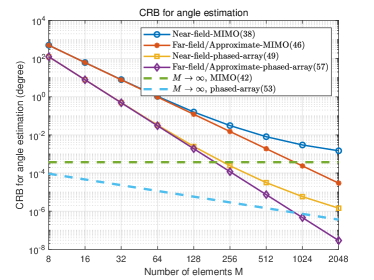
Figure 2: CRB of angle for monostatic sensing.

Fig.2 and Fig.3 plot the CRBs of angle $\theta$ and range $r$ versus the number of antennas $M$ for various models, as given in (38)-(39), (49)-(50), (42) and (53), respectively. In this case, the target range is set to be $r=10$m, while the angle is $\theta=\pi/6$. The legend “Near-field-MIMO” and “Near-field-phased array” denote the general expression of CRBs in (38), (39), (49) and (50), while “Approximate-MIMO” and “Approximate-phased array” denote the CRBs based on the second-order Taylor approximation in (46), (47), (57) and (58), respectively. Besides, “Far-field-MIMO” and “Far-field-phased array” denote CRBs of the conventional UPW model, respectively. The dotted lines are the asymptotic limits when $\frac{D_{T}}{r\cos\theta}\to\infty$.

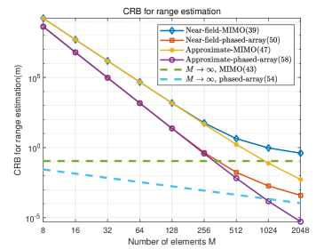
Figure 3: CRB of range for monostatic sensing. For conventional UPW model, CRB of range is $\infty$.

Fig.2 shows that the CRBs for angle of phased array radar mode is smaller than that of MIMO radar mode, since the former usually benefits from an additional transmit beamforming gain. Besides, the CRBs of angle for both XL-MIMO radar and XL-phased array radar decrease with the increase of antenna size, but with diminishing return. Furthermore, for relatively small $M$ values, the CRBs of angle for XL-MIMO and XL-phased array radar are consistent with the far-field CRBs. However, with the increasing of antenna number, the two models lead to dramatical different results. This indicates that using inappropriate far-field model to analyse near-field sensing with extremely large-scale arrays may cause severe errors. Furthermore, it is observed from Fig. 3 that the range CRBs also decrease with the number of antenna elements. Besides, for moderate antenna number, say $M<64$, the CRBs of range are quite large. It is observed that the second-order Taylor approximation as (46)-(47) and (57)-(58) is accurate for moderate $M$, but would lead to large errors when $M$ is large.

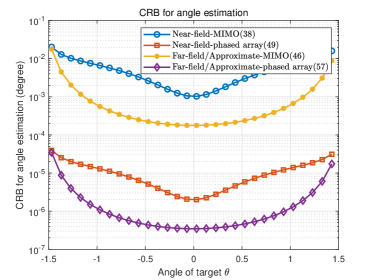
Figure 4: CRB of angle for monostatic sensing.

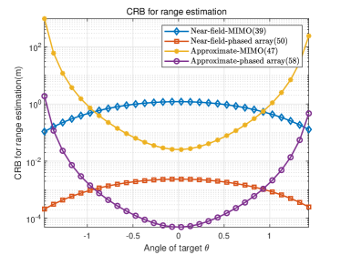
Figure 5: CRB of range for monostatic sensing.

Fig.4 and Fig.5 plot the CRBs of angle and range versus the target angle $\theta$. The number of antenna elements is set to be $M=1024$, while the target range is $r=10$m. Fig.4 shows that the CRB of angle increases with$\ |\theta|,\$and the largest CRB occurs at the boresight of the array. Besides, for the considered setup, using second-order Taylor approximation or far-field UPW model may cause $20$dB error on average, which is nonnegligible in practice. Furthermore, Fig.5 shows that CRBs based on the second-order Taylor approximation have the opposite trend compared with the CRBs based on the exact distances, which indicates that using second-order Taylor approximation would be inaccurate for near-field CRB for range.

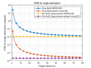
Figure 6: CRB of angle for monostatic sensing.

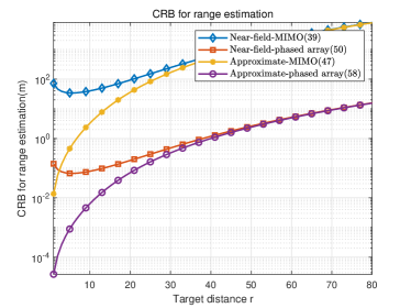
Figure 7: CRB of range for monostatic sensing.

Fig.6 and Fig.7 plot the CRBs of angle and range versus the target range $r$. The number of antenna elements is set to be $M=1024$, while target angle is $\theta=\pi/6$. Fig.6 shows that the CRB of angle decreases with the increasing of target range. Besides, for large target range $r$, the newly developed near-field CRB matches with that from the conventional UPW models. However, they deviate significantly for relatively small $r$, where far-field UPW assumption no longer holds. Fig.7 shows that the developed near-field CRB for range merges with the conventional result when the range $r$ is large. Besides, as $r$ increases, the derived CRB of range based on the exact distance first decreases and then increases, while for second-order Taylor approximation model, the CRB increases monotonically. This shows that the second-order Taylor approximation model is less accurate for smaller target range $r$.

V-B Bistatic Sensing

In this subsection, bistatic near-field sensing results are presented. corresponding to section IV-A, near-field USW model is considered only at the transmitter side and the number of the receive antenna elements is set to be $N=8$. The target angle is $\theta=0$, and the target range is $r=18$m. The transmit and receive array distance is $R=35$m. The classic Capon algorithm is used to actually estimate the parameters $\theta$ and $r$, and the performance is evaluated in terms of the root mean square error (RMSE) in the following way[39]

$$\ RMSE_{i}=\sqrt{\frac{1}{K}\sum\limits_{k=1}^{K}{{{({{\bm{\theta}_{i}}-{\bm{\hat{\theta}}_{i}}})}^{2}}}},i=1,2,$$ (74)

where$\ {\bm{\theta}_{i}}=[\theta,r],\$and $\bm{\hat{\theta}}_{i}$ denotes the estimate value of $\theta$ and $r$. $K$ is the total number of experiment, and we set $K=500$.

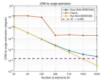
Figure 8: CRB of angle for bistatic sensing.

Fig.8 and Fig.9 plot the CRBs of angle and range versus the transmit antenna number $M$. It is observed that our derived CRBs are indeed the lower bounds for the RMSE of the Capon algorithms. Besides, the developed near-field CRB perfectly match with the far-field model when $M$ is relatively small.

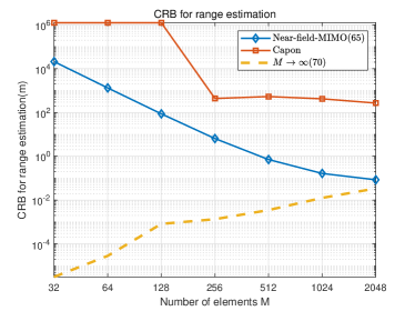
Figure 9: CRB of range for bistatic sensing.

VI Conclusion

This paper studied near-field radio sensing with extremely large-scale antenna arrays, where the USW model was considered. We considered two radar modes, namely XL-MIMO radar and XL-phased array radar modes. For the monostatic near-field sensing, the closed-form expressions of the CRBs for angle and range estimation were derived. Several asymptotic cases were also considered. It was revealed that different from the conventional far-field sensing with UPW model, the CRB for near-field angle estimation no longer decreases indefinitely as the antenna size increases. Moreover, the CRB for range estimation was shown to be finite in the near-field case, which shows the capability for range discrimination with XL-MIMO sensing. We then considered the general bistatic case and compared our derived CRBs with the classic Capon algorithm. Numerical results validated our derived CRBs.

Appendix A
Proof of Proposition 1

As shown in (33)-(37), the different parameters share some common summations. Therefore, similar to [32], in order to obtain closed-form expressions, we first define the function$\ {f_{1}}(x)\buildrel\Delta\over{=}\frac{{{x^{2}}}}{{{x^{2}}-2(\sin\theta)x+1}},\$where$\ x\in[{-\frac{{M{\varepsilon_{T}}}}{2},\frac{{M{\varepsilon_{T}}}}{2}}].\$Since$\ {\varepsilon_{T}}\ll 1,\$we have$\ f_{1}(x)\approx f_{1}(m{\varepsilon_{T}}),~{}\forall x\in[{({m-\frac{1}{2}}){\varepsilon_{T}},({m+\frac{1}{2}}){\varepsilon_{T}}}],~{}m=-\frac{{M-1}}{2},...,\frac{{M-1}}{2}.\$So we have

$$\ \sum\nolimits_{m=-\frac{{M-1}}{2}}^{\frac{{M-1}}{2}}{f_{1}(m{\varepsilon_{T}}){\varepsilon_{T}}}\approx\int_{-\frac{{M{\varepsilon_{T}}}}{2}}^{\frac{{M{\varepsilon_{T}}}}{2}}{f_{1}(x)dx}.$$ (75)

Therefore, the summation (28) and (31) can be expressed as

$$\footnotesize\begin{aligned} &\sum\nolimits_{m=-\frac{{M-1}}{2}}^{\frac{{M-1}}{2}}{\frac{{{{({m{\varepsilon_{T}}})}^{2}}}}{{1-2m{\varepsilon_{T}}\sin\theta+{{(m{\varepsilon_{T}})}^{2}}}}}\\ &\approx\frac{1}{{{\varepsilon_{T}}}}\int_{-\frac{{M{\varepsilon_{T}}}}{2}}^{\frac{{M{\varepsilon_{T}}}}{2}}{\frac{{{x^{2}}}}{{{x^{2}}-2(\sin\theta)x+1}}}dx\\ &=M+\frac{{\sin\theta}}{{{\varepsilon_{T}}}}\int_{-\frac{{M{\varepsilon_{T}}}}{2}}^{\frac{{M{\varepsilon_{T}}}}{2}}{\frac{1}{{{x^{2}}-2(\sin\theta)x+1}}}d({{x^{2}}-2(\sin\theta)x+1})\\ &-\frac{\cos 2\theta}{{{\varepsilon_{T}}}}\int_{-\frac{{M{\varepsilon_{T}}}}{2}}^{\frac{{M{\varepsilon_{T}}}}{2}}{\frac{1}{{{x^{2}}-2(\sin\theta)x+1}}}dx\\ &\mathop{=}\limits^{(a)}M+\frac{{\sin\theta}}{{{\varepsilon_{T}}}}\ln\left|{\frac{{\frac{{D_{T}^{2}}}{{4{r^{2}}}}-\sin\theta\frac{{{D_{T}}}}{r}+1}}{{\frac{{D_{T}^{2}}}{{4{r^{2}}}}+\sin\theta\frac{{{D_{T}}}}{r}+1}}}\right|-\frac{{\cos 2\theta}}{{{\varepsilon_{T}}\cos\theta}}\Delta_{{\rm{span}}}^{\rm{t}}\left(\frac{{{D_{T}}}}{r}\right),\end{aligned}\$$ (76)

where$\ \Delta_{{\rm{span}}}^{t}(\frac{{{D_{T}}}}{r})=\arctan({\frac{{{D_{T}}}}{{{\rm{2}}r\cos\theta}}-\tan\theta})+\arctan({\frac{{{D_{T}}}}{{{\rm{2}}r\cos\theta}}+\tan\theta})\$is the transmit angular span[32]. $(a)$ in (76) follows from the integral formula 2.103 in [18], i.e.,$\ \int{\frac{{(Mx+N)dx}}{{A+2Bx+C{x^{2}}}}=\frac{M}{{2C}}\ln\left|{A+2Bx+C{x^{2}}}\right|}+\frac{{NC-MB}}{{C\sqrt{AC-{B^{2}}}}}\arctan\frac{{Cx+B}}{{\sqrt{AC-{B^{2}}}}}\$for$\ AC>{B^{2}},\$and the fact that $\sin^{2}\theta\leq 1$ in (76). Therefore, the closed-form expression of the parameter $a$ and $p$ can be derived by substituting (76) in (33) and (36).

Similarly, we define the functions$\ {f_{2}}(x)\buildrel\Delta\over{=}\frac{x}{{\sqrt{{x^{2}}-2(\sin\theta)x+1}}}\$and$\ {f_{3}}(x){\rm{}}\buildrel\Delta\over{=}\frac{x}{{{x^{2}}-2(\sin\theta)x+1}},\$and the summation in (29) and (32) can be expressed as

$$\sum\nolimits_{m=-\frac{{M-1}}{2}}^{\frac{{M-1}}{2}}{\frac{{m{\varepsilon_{T}}}}{{\sqrt{1-2m{\varepsilon_{T}}\sin\theta+{{(m{\varepsilon_{T}})}^{2}}}}}}$$ (77)

$$\approx\frac{1}{{{\varepsilon_{T}}}}\int_{-\frac{{M{\varepsilon_{T}}}}{2}}^{\frac{{M{\varepsilon_{T}}}}{2}}{\frac{x}{{\sqrt{{x^{2}}-2\sin(\theta)x+1}}}}dx$$

$$=\frac{1}{{{\varepsilon_{T}}}}\left[{\sqrt{\frac{{D_{T}^{2}}}{{4{r^{2}}}}-\sin\theta\frac{{{D_{T}}}}{r}+1}}-{\sqrt{\frac{{D_{T}^{2}}}{{4{r^{2}}}}+\sin\theta\frac{{{D_{T}}}}{r}+1}}\right.$$

$$\left.+\psi\left(\frac{D_{T}}{r}\right)\sin\theta\right],$$

where$~{}\psi(\frac{{{D_{T}}}}{r})\triangleq\ln\left(\frac{{{p_{2}}+\sqrt{1+p_{2}^{2}}}}{{{p_{1}}+\sqrt{1+p_{1}^{2}}}}\right)$ with$\ {p_{1}}=\frac{{-\frac{{{D_{T}}}}{{2r}}-\sin\theta}}{{\cos\theta}},~{}{p_{2}}=\frac{{\frac{{{D_{T}}}}{{2r}}-\sin\theta}}{{\cos\theta}},\$and the summation in (30)

$$\sum\nolimits_{m=-\frac{{M-1}}{2}}^{\frac{{M-1}}{2}}{\frac{{m{\varepsilon_{T}}}}{{1-2m{\varepsilon_{T}}\sin\theta+{{(m{\varepsilon_{T}})}^{2}}}}}$$ (78)

$$\approx\frac{1}{{{\varepsilon_{T}}}}\int_{-\frac{{M{\varepsilon_{T}}}}{2}}^{\frac{{M{\varepsilon_{T}}}}{2}}{\frac{x}{{{x^{2}}-2\sin(\theta)x+1}}}dx$$

$$=\frac{1}{{2{\varepsilon_{T}}}}\ln\left|{\frac{{\frac{{D_{T}^{2}}}{{4{r^{2}}}}-\sin\theta\frac{{{D_{T}}}}{r}+1}}{{\frac{{D_{T}^{2}}}{{4{r^{2}}}}+\sin\theta\frac{{{D_{T}}}}{r}+1}}}\right|+\frac{{\sin\theta}}{{{\varepsilon_{T}}\cos\theta}}\Delta_{{\rm{span}}}^{\rm{t}}\left(\frac{{{D_{T}}}}{r}\right).$$

By substituting (76) and (78) into (35) and (36), the closed-form expressions of parameters $e$ and $p$ can be obtained accordingly. Furthermore, by substituting (77) into (34) and (37), $c$ and $q$ in Proposition 1 can be obtained accordingly.

Appendix B
Proof of Corollary 1.1

By noting that the parameters in (33)-(37) involve some common terms, we first define the following four functions:

$${g_{1}}\left({\frac{{{D_{T}}}}{r}}\right) \triangleq\sqrt{\frac{{{D_{T}}^{2}}}{{4{r^{2}}}}-\frac{{{D_{T}}}}{r}\sin\theta+1}-\sqrt{\frac{{{D_{T}}^{2}}}{{4{r^{2}}}}+\frac{{{D_{T}}}}{r}\sin\theta+1},$$ (79)

$${g_{2}}\left({\frac{{{D_{T}}}}{r}}\right) \triangleq\Delta_{{\rm{span}}}^{\rm{t}}\left(\frac{{{D_{T}}}}{r}\right),{g_{3}}\left({\frac{{{D_{T}}}}{r}}\right)\triangleq\ln\left|{\frac{{\frac{{{D_{T}}^{2}}}{{4{r^{2}}}}-\frac{{{D_{T}}}}{r}\sin\theta+1}}{{\frac{{{D_{T}}^{2}}}{{4{r^{2}}}}+\frac{{{D_{T}}}}{r}\sin\theta+1}}}\right|,$$

$${g_{4}}\left({\frac{{{D_{T}}}}{r}}\right) \triangleq\ln\left(\frac{{{p_{2}}+\sqrt{1+p_{2}^{2}}}}{{{p_{1}}+\sqrt{1+p_{1}^{2}}}}\right),$$

where $\ {p_{1}}=\frac{{-\frac{{{D_{T}}}}{{2r}}-\sin\theta}}{{\cos\theta}},\$and$\ {p_{2}}=\frac{{\frac{{{D_{T}}}}{{2r}}-\sin\theta}}{{\cos\theta}},\$as given in Proposition 1. When $\frac{{{D_{T}}}}{r}\gg 1,\$as in Corollary 1.1, we have

$${{g_{1}}\left({\frac{{{D_{T}}}}{r}}\right)} =\frac{{{D_{T}}}}{{2r}}{\left({\sqrt{1+\frac{{4{r^{2}}}}{{{D_{T}}^{2}}}-\frac{4r\sin\theta}{{{D_{T}}}}}-\sqrt{1+\frac{{4{r^{2}}}}{{{D_{T}}^{2}}}+\frac{4r\sin\theta}{{{D_{T}}}}}}\right)}$$ (80)

$$\mathop{\approx}\limits^{(a)}\frac{{{D_{T}}}}{{2r}}\left(-\frac{4r}{{{D_{T}}}}\sin\theta\right)=-2\sin\theta,$$

where $(a)$ in (80) follows from the first-order Taylor approximation with $\frac{r}{D_{T}}\ll 1$. Besides, it was shown in [32] that$\ {g_{2}}\left({\frac{{{D_{T}}}}{r}}\right)=\Delta_{{\rm{span}}}^{\rm{t}}(\frac{{{D_{T}}}}{r})\approx\pi.\$Similarly,$\ {g_{3}}\left({\frac{{{D_{T}}}}{r}}\right)\$can be obtained as

$$\footnotesize\begin{aligned} {g_{3}}\left({\frac{{{D_{T}}}}{r}}\right)&=\ln\left|{1-\frac{{2\frac{{{D_{T}}}}{r}\sin\theta}}{{\frac{{{D_{T}}^{2}}}{{4{r^{2}}}}+\frac{{{D_{T}}}}{r}\sin\theta+1}}}\right|\approx 0.\end{aligned}\$$ (81)

Furthermore, the last term$\ {g_{4}}\left({\frac{{{D_{T}}}}{r}}\right)\$can be expressed as

$${{g_{4}}\left({\frac{{{D_{T}}}}{r}}\right)} \mathop{\approx}\limits^{(d)}\ln\left({\frac{{\frac{{{D_{T}}}}{{2r\cos\theta}}+\sqrt{1+{{({\frac{{{D_{T}}}}{{2r\cos\theta}}})}^{2}}}}}{{-\frac{{{D_{T}}}}{{2r\cos\theta}}+\sqrt{1+{{({\frac{{{D_{T}}}}{{2r\cos\theta}}})}^{2}}}}}}\right)\approx 2\ln\left({\frac{{{D_{T}}}}{{r\cos\theta}}}\right),$$ (82)

where $(d)$ follows from$\ \frac{{\frac{{{D_{T}}}}{{2r}}-\sin\theta}}{{\cos\theta}}\approx\frac{{{D_{T}}}}{{2r\cos\theta}}\$when $D_{T}/r\gg 1.$

Note that the parameter $a$ in (33) can be written based on $g_{2}$ and $g_{3}$ defined above. Therefore, when $D_{T}/r\gg 1,$ by substituting $g_{2}$ and $g_{3}$ into (33), we have

$$a =\frac{{4{\pi^{2}}{r^{2}}{{\cos}^{2}}\theta}}{{{\lambda^{2}}{\varepsilon_{T}}}}\left({\frac{{{D_{T}}}}{r}+{g_{3}}\sin\theta-{g_{2}}\frac{{\cos 2\theta}}{{\cos\theta}}}\right)$$ (83)

$$=\frac{{4{\pi^{2}}{r^{2}}{{\cos}^{2}}\theta}}{{{\lambda^{2}}{\varepsilon_{T}}}}\left({\frac{{{D_{T}}}}{r}-\frac{{\cos 2\theta}}{{\cos\theta}}\pi}\right).$$

Similarly, other parameters $e,c,p,q$ can be written based on $g_{1},g_{2},g_{3}$ and $g_{4}$ and when $D_{T}/r\gg 1$, we have

$$e =\frac{{2{\pi^{2}}r\sin 2\theta}}{{{\lambda^{2}}{\varepsilon_{T}}}}\left({\frac{{{D_{T}}}}{r}-2\pi\cos\theta}\right),$$ (84)

$$p =\frac{{4{\pi^{2}}}}{{{\lambda^{2}}{\varepsilon_{T}}}}\left({\frac{{{D_{T}}}}{r}{{\sin}^{2}}\theta+\pi\cos\theta\cos 2\theta}\right),$$

$$c =-j\frac{{2\pi r\sin 2\theta}}{{\lambda{\varepsilon_{T}}}}\left[{\ln\left({\frac{{{D_{T}}}}{{r\cos\theta}}}\right)-1}\right],$$

$$q =j\frac{{4\pi}}{{\lambda{\varepsilon_{T}}}}\left[{{{\cos}^{2}}\theta\ln\left({\frac{{{D_{T}}}}{{r\cos\theta}}}\right)+{{\sin}^{2}}\theta}\right].$$

By substituting these terms into (38) and (39), the expressions in (40) and (41) can be obtained accordingly.

Appendix C
Proof of Corollary 1.2

When $\frac{D_{T}}{r\cos\theta}\to\infty$, the constant terms in (40) and (41) can be neglected. Therefore, we have the simplified results in (42) and (43) by some simple algebraic calculation:

$$CR{B_{\theta}} \approx\frac{1}{{2\gamma L}}$$ (85)

$$\frac{{{\lambda^{2}}\left[\frac{{{{\sin}^{2}}2\theta}}{4}{{(\frac{{{D_{T}}}}{{r\cos\theta}})}^{2}}+\frac{{\pi{D_{T}}}}{{r\cos\theta}}{{\cos}^{2}}\theta\cos 2\theta-4{{({{\cos}^{2}}\theta\ln\frac{{{D_{T}}}}{{r\cos\theta}})}^{2}}\right]}}{{8{\pi^{2}}M{r^{2}}{{\cos}^{2}}\theta(\frac{{\pi{D_{T}}}}{r{\cos\theta}}-4{{\ln}^{2}}\frac{{{D_{T}}}}{{r\cos\theta}})}}$$

$$\mathop{\approx}\limits^{(g)}\frac{1}{{2\gamma}}\frac{{{\lambda^{2}}{{(\frac{{{D_{T}}}}{r})}^{2}}{{\sin}^{2}}\theta}}{{8{\pi^{2}}{r^{2}}M{{\cos}^{2}}\theta\frac{{\pi{D_{T}}}}{r{\cos\theta}}}}\approx\frac{1}{{2\gamma}}\frac{{{\lambda^{2}}{d_{T}}{{\sin}^{2}}\theta}}{{8{\pi^{3}}{r^{3}}\cos\theta}},$$

$$CR{B_{r}} \approx\frac{1}{{2\gamma L}}\frac{{{\lambda^{2}}\left[{{\cos}^{2}}\theta{{(\frac{{{D_{T}}}}{{r\cos\theta}})}^{2}}+\frac{\pi{D_{T}}{\cos 2\theta}}{r{\cos\theta}}-4{{\sin}^{2}}\theta{{(\ln\frac{{{D_{T}}}}{{r\cos\theta}})}^{2}}\right]}}{{8{\pi^{2}}M(\frac{{\pi{D_{T}}}}{r{\cos\theta}}-4{{\ln}^{2}}\frac{{{D_{T}}}}{{r\cos\theta}})}}$$

$$\mathop{\approx}\limits^{(g)}\frac{1}{{2\gamma}}\frac{{{\lambda^{2}}{{(\frac{{{D_{T}}}}{r})}^{2}}}}{{8{\pi^{2}}M\frac{{\pi{D_{T}}}}{r{\cos\theta}}}}\approx\frac{1}{{2\gamma}}\frac{{{\lambda^{2}}{d_{T}}\cos\theta}}{{8{\pi^{3}}r}},$$

where $(g)$ follows from$\ \mathop{\lim}\limits_{x\to\infty}\left({a{x^{2}}+bx-c{{\ln}^{2}}x}\right)=a{x^{2}},\$$\ \mathop{\lim}\limits_{x\to\infty}\left({bx-c{{\ln}^{2}}x}\right)=bx,\$with $x=\frac{D_{T}}{r\cos\theta}$.

Appendix D
Proof of Corollary 1.3

Similar to the derivation in Appendix B, when $D_{T}/r\ll 1$, the functions $g_{1},~{}g_{2},~{}g_{3},~{}g_{4}$ in Appendix B reduce to

$${g_{1}}\left({\frac{{{D_{T}}}}{r}}\right) \mathop{\approx}\limits^{(h1)}-\frac{{{D_{T}}}}{r}\sin\theta,~{}{g_{2}}\left({\frac{{{D_{T}}}}{r}}\right)\mathop{\approx}\limits^{(h2)}\frac{{{D_{T}}}}{r}\cos\theta-\frac{{{{\cos}^{3}}\theta}}{{12}}{\left({\frac{{{D_{T}}}}{r}}\right)^{3}},$$ (86)

$${g_{3}}\left({\frac{{{D_{T}}}}{r}}\right) \mathop{\approx}\limits^{(h3)}-2\frac{{{D_{T}}}}{r}\sin\theta+\frac{{\sin\theta}}{2}{\left({\frac{{{D_{T}}}}{r}}\right)^{3}},~{}{g_{4}}\left({\frac{{{D_{T}}}}{r}}\right)\mathop{\approx}\limits^{(h4)}\frac{{{D_{T}}}}{r},$$

where $(h1)$ and $(h4)$ follow from the first-order Taylor approximation, and $(h2)$ and $(h3)$ follow from the third-order and second-order Taylor approximation. Note that $(h1)$ and $(h4)$ are related to $c$ and $q$, which only appear in the form of square, so there is no need to consider higher order approximation when $D_{T}/r\ll 1$. By substituting (86) into (33)-(37), the closed form expressions of intermediate parameters $a,e,p,c,q$ are obtained. By substituting (86) into (38), the CRB expression in (45) can be obtained.

Appendix E
Proof of Corollary 1.4

The second-order Taylor approximation of the distance between the target and the $m$th antenna element in (1) is

$${r_{m}}\approx r+\frac{1}{{2r}}{({m{d_{T}}})^{2}}{\cos^{2}}\theta-m{d_{T}}\sin\theta.$$ (87)

Therefore, the element of the steering vector ${a_{m}}(\theta,r)$ in (5) can be expressed as ${{a_{m}}(\theta,r)={e^{jmv+j{m^{2}}\phi-j\frac{{2\pi}}{\lambda}r}}},\$where$\ v=\frac{{2\pi{d_{T}}\sin\theta}}{\lambda}$, $\phi=-\frac{{\pi{{d_{T}}^{2}}{{\cos}^{2}}\theta}}{{\lambda r}}.\$The derivatives of angle and range of steering vector are

$$\frac{{\partial{a_{m}}(r,\theta)}}{{\partial\theta}} ={e^{jmv+j{m^{2}}\phi-j\frac{{2\pi}}{\lambda}r}}\left({jm\frac{{\partial v}}{{\partial\theta}}+j{m^{2}}\frac{{\partial\phi}}{{\partial\theta}}}\right),$$ (88)

$$\frac{{\partial{a_{m}}(r,\theta)}}{{\partial r}} ={e^{jmv+j{m^{2}}\phi-j\frac{{2\pi}}{\lambda}r}}\left({j{m^{2}}\frac{{\partial\phi}}{{\partial r}}-j\frac{{2\pi}}{\lambda}}\right),$$

where $\frac{{\partial v}}{{\partial\theta}}=\frac{{2\pi{d_{T}}\cos\theta}}{\lambda},\frac{{\partial\phi}}{{\partial\theta}}=\frac{{\pi{d_{T}}^{2}\sin 2\theta}}{{\lambda r}},\$and$\ \frac{{\partial\phi}}{{\partial r}}=\frac{{\pi{d_{T}}^{2}{{\cos}^{2}}\theta}}{{\lambda{r^{2}}}}.$ Therefore, the intermediate parameters $a,c,e,p,q$ based on the second-order Taylor approximation model can be derived as

$$a ={{{\left\|{\frac{{\partial{\bf{a}}(r,\theta)}}{{\partial\theta}}}\right\|}^{2}}=\sum\nolimits_{m=-\frac{{M-1}}{2}}^{\frac{{M-1}}{2}}{{m^{2}}{\left({\frac{{2\pi{d_{T}}\cos\theta}}{\lambda}+m\frac{{\pi{{d_{T}}^{2}}\sin{2\theta}}}{{\lambda r}}}\right)^{2}}}}$$ (89)

$$={\left({\frac{{2\pi{d_{T}}\cos\theta}}{\lambda}}\right)^{2}}{\eta_{1}}+{\left({\frac{{\pi{{d_{T}}^{2}}\sin{2\theta}}}{{\lambda r}}}\right)^{2}}{\eta_{2}},$$

where$\ {\eta_{1}}=\sum\nolimits_{m=-\frac{{M-1}}{2}}^{\frac{{M-1}}{2}}{{m^{2}}}=\frac{{M({{M^{2}}-1})}}{12}\$and$\ {\eta_{2}}=\sum\nolimits_{m=-\frac{{M-1}}{2}}^{\frac{{M-1}}{2}}{{m^{4}}}=\frac{{M({{M^{2}}-1})({3{M^{2}}-7})}}{{240}}.\$Similarly, we can obtain other parameters:

$$p ={{\left({\frac{{\pi{{d_{T}}^{2}}{{\cos}^{2}}\theta}}{{\lambda{r^{2}}}}}\right)}^{2}}{\eta_{2}}-{{\left({\frac{{2\pi{d_{T}}\cos\theta}}{\lambda r}}\right)}^{2}}{\eta_{1}}+\frac{{4{\pi^{2}}}}{{{\lambda^{2}}}}M,$$ (90)

$$e =\left({\frac{{{\pi^{2}}{{d_{T}}^{4}}{{\cos}^{2}}\theta\sin 2\theta}}{{{\lambda^{2}}{r^{3}}}}}\right){\eta_{2}}-\frac{{2{\pi^{2}}{{d_{T}}^{2}}\sin 2\theta}}{{{\lambda^{2}}r}}{\eta_{1}},$$

$$c =-j\frac{{\pi{{d_{T}}^{2}}\sin 2\theta}}{{\lambda r}}{\eta_{1}},q=-j\frac{{\pi{{d_{T}}^{2}}{{\cos}^{2}}\theta}}{{\lambda{r^{2}}}}{\eta_{1}}+j\frac{{2\pi}}{\lambda}M.$$

By substituting (90) into (38)-(39), the expressions in (46) and (47) can be obtained accordingly.

Appendix F
Proof of Corollary 3.1

When $\theta=0$, the parameters in (62) reduce to

$${\Gamma_{\theta}}(r,\theta)=\frac{r}{{R-r}},~{}{\Gamma_{r}}(r,\theta)=0.$$ (91)

Therefore, the parameters in (64) and (65) reduce to

$$a =\frac{{4{\pi^{2}}{r^{2}}}}{{{\lambda^{2}}{\varepsilon_{T}}}}\left[{\frac{{{D_{T}}}}{r}}\right.\left.{-2\arctan\left({\frac{{{D_{T}}}}{{2r}}}\right)}\right],~{}c=e=s=k=f=h=0,$$ (92)

$$p =\frac{{4{\pi^{2}}}}{{{\lambda^{2}}{\varepsilon_{T}}}}2\arctan\left({\frac{{{D_{T}}}}{{2r}}}\right),~{}q=j\frac{{2\pi}}{{\lambda{\varepsilon_{T}}}}\ln\left({\frac{{\frac{{{D_{T}}}}{{2r}}+\sqrt{1+{{\left({\frac{{{D_{T}}}}{{2r}}}\right)}^{2}}}}}{{-\frac{{{D_{T}}}}{{2r}}+\sqrt{1+{{\left({\frac{{{D_{T}}}}{{2r}}}\right)}^{2}}}}}}\right),$$

$$i =\frac{{{\pi^{2}}d_{R}^{2}{r^{2}}}}{{3{\lambda^{2}}{{(R-r)}^{2}}}}N({N^{2}}-1),$$

Therefore, the CRBs in (64) and (65) reduce to

$$CR{B_{\theta}}=\frac{1}{{2\gamma L}}\frac{M}{{Mi+Na}},~{}CR{B_{r}}=\frac{1}{{2\gamma LN}}\frac{M}{{p-\frac{1}{M}{{\left|q\right|}^{2}}}}.$$ (93)

By substituting (92) in (93), the closed-form expressions in (67) and (68) can be obtained. In order to obtain the minimal point of range CRB, the derivative of $CRB_{r}$ with respect to $\frac{D_{T}}{2r}$ is derived. Let $x=\frac{D_{T}}{2r}$, and the derivative can be expressed as

$$\frac{{\partial CR{B_{r}}}}{{\partial x}}=\frac{{{\lambda^{2}}}}{{8{\pi^{2}}\gamma LN}}$$ (94)

$$\times\frac{{\arctan x-\frac{x}{{1+{x^{2}}}}+\frac{2}{{\sqrt{1+{x^{2}}}}}\ln\left({x+\sqrt{1+{x^{2}}}}\right)-\frac{2}{x}{{\ln}^{2}}\left({x+\sqrt{1+{x^{2}}}}\right)}}{{{{\left[{\arctan x-\frac{1}{x}{{\ln}^{2}}\left({x+\sqrt{1+{x^{2}}}}\right)}\right]}^{2}}}}$$

In order to obtain the minimal point, let$\ \frac{{\partial CR{B_{r}}}}{{\partial x}}=0\$and solution is $x\approx 6$ by numerical simulation, i.e., $D_{T}\approx 12r$.

References

• [1] H. Wang and Y. Zeng, “SNR scaling laws for radio sensing with extremely large-scale MIMO,” in Proc. IEEE Int. Conf. Commun. Workshops (ICC Workshops), 2022, pp. 121–126.
• [2] M. Latva-aho and K. L. (eds.), “Key drivers and research challenges for 6G ubiquitous wireless intelligence,” 6G Research Visions 1, 6G Flagship, University of Oulu, Finland, Sep. 2019.
• [3] X. You et al., “Towards 6G wireless communication networks: Vision, enabling technologies, and new paradigm shifts,” Sci. China Inf. Sci., vol. 64, no. 1, pp. 1–74, Nov. 2020.
• [4] Y. Zeng and X. Xu, “Toward environment-aware 6G communications via channel knowledge map,” IEEE Wireless Commun., pp. 1–8, Mar. 2021.
• [5] M. L. Rahman, J. A. Zhang, X. Huang, Y. J. Guo, and R. W. Heath, “Framework for a perceptive mobile network using joint communication and radar sensing,” IEEE Trans. Aerosp. Electron. Syst., vol. 56, no. 3, pp. 1926–1941, Jun. 2020.
• [6] J. A. Zhang, F. Liu, C. Masouros, R. W. Heath, Z. Feng, L. Zheng, and A. Petropulu, “An overview of signal processing techniques for joint communication and radar sensing,” IEEE J. Sel. Top. Sign. Proces., vol. 15, no. 6, pp. 1295–1315, 2021.
• [7] Z. Xiao and Y. Zeng, “An overview on integrated localization and communication towards 6G,” Sci. China Inf. Sci., vol. 65, no. 3, pp. 1–46, 2022.
• [8] F. Liu, C. Masouros, A. Li, H. Sun, and L. Hanzo, “MU-MIMO communications with MIMO radar: From co-existence to joint transmission,” IEEE Trans. Wireless Commun., vol. 17, no. 4, pp. 2755–2770, Apr. 2018.
• [9] A. Hassanien, M. G. Amin, E. Aboutanios, and B. Himed, “Dual-function radar communication systems: A solution to the spectrum congestion problem,” IEEE Signal Process. Mag., vol. 36, no. 5, pp. 115–126, 2019.
• [10] Y. Cui, F. Liu, X. Jing, and J. Mu, “Integrating sensing and communications for ubiquitous IoT: Applications, trends, and challenges,” IEEE Netw., vol. 35, no. 5, pp. 158–167, 2021.
• [11] F. Liu, C. Masouros, T. Ratnarajah, and A. Petropulu, “On range sidelobe reduction for dual-functional radar-communication waveforms,” IEEE Wireless Commun. Lett., vol. 9, no. 9, pp. 1572–1576, 2020.
• [12] C. Sturm and W. Wiesbeck, “Waveform design and signal processing aspects for fusion of wireless communications and radar sensing,” Proc. IEEE, vol. 99, no. 7, pp. 1236–1259, 2011.
• [13] Y. Liu, G. Liao, J. Xu, Z. Yang, and Y. Zhang, “Adaptive OFDM integrated radar and communications waveform design based on information theory,” IEEE Commun. Lett., vol. 21, no. 10, pp. 2174–2177, 2017.
• [14] P. Kumari, S. A. Vorobyov, and R. W. Heath, “Adaptive virtual waveform design for millimeter-wave joint communication–radar,” IEEE Trans. Signal Process., vol. 68, pp. 715–730, 2020.
• [15] Z. Xiao and Y. Zeng, “Waveform design and performance analysis for full-duplex integrated sensing and communication,” IEEE J. Sel. Areas Commun., vol. 40, no. 6, pp. 1823–1837, 2022.
• [16] S. Chen, A. Kaushik, and C. Masouros, “Pre-scaling and codebook design for joint radar and communication based on index modulation,” in Proc. IEEE Glob. Commun. Conf., GLOBECOM - Proc., 2022, pp. 6037–6041.
• [17] S. Chen, Z. Xiao, and Y. Zeng, “Simultaneous beam sweeping for multi-beam integrated sensing and communication,” in Proc. IEEE Int. Conf. Commun. (ICC), 2022, pp. 4438–4443.
• [18] W. Chen, L. Li, Z. Chen, T. Quek, and S. Li, “Enhancing THz/mmWave network beam alignment with integrated sensing and communication,” IEEE Commun. Lett., vol. 26, pp. 1698 – 1702, 2022.
• [19] M. Kobayashi, G. Caire, and G. Kramer, “Joint state sensing and communication: Optimal tradeoff for a memoryless case,” in Proc. IEEE Int. Symp. Inf. Theor. Proc., 2018, pp. 111–115.
• [20] M. Kobayashi, H. Hamad, G. Kramer, and G. Caire, “Joint state sensing and communication over memoryless multiple access channels,” in Proc. IEEE Int. Symp. Inf. Theor. Proc., 2019, pp. 270–274.
• [21] A. Liu, Z. Huang, M. Li, Y. Wan, W. Li, T. X. Han, C. Liu, R. Du, D. K. P. Tan, J. Lu et al., “A survey on fundamental limits of integrated sensing and communication,” IEEE Commun. Surv. Tutor., vol. 24, no. 2, pp. 994–1034, 2022.
• [22] H. Cramér, Mathematical methods of statistics.   Princeton university press, 1999, vol. 43.
• [23] H. L. Van Trees and K. L. Bell, “Bayesian bounds for parameter estimation and nonlinear filtering/tracking,” AMC, vol. 10, no. 12, pp. 10–1109, 2007.
• [24] V. M. Chiriac, Q. He, A. M. Haimovich, and R. S. Blum, “Ziv–zakai bound for joint parameter estimation in MIMO radar systems,” IEEE Trans. Signal Process., vol. 63, no. 18, pp. 4956–4968, 2015.
• [25] J. Li and P. Stoica, MIMO Radar Signal Processing.   John Wiley & Sons, Ltd, 2009.
• [26] R. Boyer, “Performance bounds and angular resolution limit for the moving colocated MIMO radar,” IEEE Trans. Signal Process., vol. 59, no. 4, pp. 1539–1552, 2011.
• [27] Q. He, R. S. Blum, H. Godrich, and A. M. Haimovich, “Cramer-Rao bound for target velocity estimation in mimo radar with widely separated antennas,” in Proc. CISS, Annu. Conf. Inf. Sci. Syst., 2008, pp. 123–127.
• [28] K. Rambach and B. Yang, “Direction of arrival estimation of two moving targets using a time division multiplexed colocated MIMO radar,” in Proc. IEEE Nat. Radar Conf. Proc., 2014, pp. 1118–1123.
• [29] M. A. Richards, Fundamentals of radar signal processing.   McGraw-Hill Education, 2014.
• [30] C. Shi, D. Xu, Y. Zhou, and W. Tu, “Range-DoA information and scattering information in phased-array radar,” in Proc. IEEE Int. Conf. Comput. Commun. (ICCC), 2019, pp. 747–752.
• [31] T. L. Marzetta, “Noncooperative cellular wireless with unlimited numbers of base station antennas,” IEEE Trans. Wireless Commun., vol. 9, no. 11, pp. 3590–3600, Nov. 2010.
• [32] H. Lu and Y. Zeng, “How does performance scale with antenna number for extremely large-scale MIMO?” in Proc. IEEE Int. Conf. Commun. (ICC), 2021, pp. 1–6.
• [33] A. Amiri, M. Angjelichinoski, E. de Carvalho, and R. W. Heath, “Extremely large aperture massive MIMO: Low complexity receiver architectures,” in Proc. IEEE Globecom Workshops, GC Wkshps - Proc., Dec. 2018, pp. 1–6.
• [34] H. Lu and Y. Zeng, “Communicating with extremely large-scale array/surface: Unified modeling and performance analysis,” IEEE Trans. Wireless Commun., vol. 21, no. 6, pp. 4039–4053, Jun. 2022.
• [35] E. Björnson and L. Sanguinetti, “Power scaling laws and near-field behaviors of massive MIMO and intelligent reflecting surfaces,” IEEE Open J. Commun. Society, vol. 1, pp. 1306–1324, Sep. 2020.
• [36] J. P. González-Coma, F. J. López-Martínez, and L. Castedo, “Low-complexity distance-based scheduling for multi-user XL-MIMO systems,” IEEE Wireless Commun. Lett., vol. 10, no. 11, pp. 2407–2411, 2021.
• [37] J. Li and P. Stoica, “MIMO radar with colocated antennas,” IEEE Signal Process. Mag., vol. 24, no. 5, pp. 106–114, Sep. 2007.
• [38] G. Liu and X. Sun, “Efficient method of passive localization for mixed far-field and near-field sources,” IEEE Antennas Wireless Propag. Lett., vol. 12, pp. 902–905, 2013.
• [39] M. N. El Korso, R. Boyer, A. Renaux, and S. Marcos, “Conditional and unconditional Cramér–Rao bounds for near-field source localization,” IEEE Trans. Signal Process., vol. 58, no. 5, pp. 2901–2907, 2010.
• [40] L. Khamidullina, I. Podkurkov, and M. Haardt, “Conditional and unconditional Cramér-Rao bounds for near-field localization in bistatic MIMO radar systems,” IEEE Trans. Signal Process., vol. 69, pp. 3220–3234, 2021.
• [41] Y. Begriche, M. Thameri, and K. Abed-Meraim, “Exact Cramer Rao bound for near field source localization,” in Proc. Int. Conf. Inf. Sci., Signal Process. Appl., (ISSPA), 2012, pp. 718–721.
• [42] A. Guerra, F. Guidi, D. Dardari, and P. M. Djurić, “Near-field tracking with large antenna arrays: Fundamental limits and practical algorithms,” IEEE Trans. Signal Process., vol. 69, pp. 5723–5738, 2021.
• [43] J. He, L. Li, T. Shu, and T.-K. Truong, “Mixed near-field and far-field source localization based on exact spatial propagation geometry,” IEEE Trans. Veh. Technol., vol. 70, no. 4, pp. 3540–3551, 2021.
• [44] J. Capon, “High-resolution frequency-wavenumber spectrum analysis,” Proc. IEEE, vol. 57, no. 8, pp. 1408–1418, 1969.
• [45] E. Björnson, ö. T. Demir, and L. Sanguinetti, “A primer on near-field beamforming for arrays and reconfigurable intelligent surfaces,” in Proc. Conf. Rec. Asilomar Conf. Signals Syst. Comput., 2021, pp. 105–112.
• [46] K. Forsythe, D. Bliss, and G. Fawcett, “Multiple-input multiple-output MIMO radar: performance issues,” in Proc. Thirty-Eighth Asilomar Conf. Signals, Systems and Computers, vol. 1, Nov. 2004, pp. 310–315.
• [47] S. Hu, F. Rusek, and O. Edfors, “Beyond massive MIMO: The potential of positioning with large intelligent surfaces,” IEEE Trans. Signal Process., vol. 66, no. 7, pp. 1761–1774, 2018.
• [48] X. Gan, C. Huang, Z. Yang, C. Zhong, and Z. Zhang, “Near-field localization for holographic RIS assisted mmWave systems,” IEEE Commun. Lett., vol. 27, no. 1, pp. 140–144, 2023.
• [49] C. Huang, S. Hu, G. C. Alexandropoulos, A. Zappone, C. Yuen, R. Zhang, M. D. Renzo, and M. Debbah, “Holographic MIMO surfaces for 6G wireless networks: Opportunities, challenges, and trends,” IEEE Wireless Commun., vol. 27, no. 5, pp. 118–125, 2020.
• [50] J. Sherman, “Properties of focused apertures in the fresnel region,” IRE Trans. Anntenas Propag., vol. 10, no. 4, pp. 399–408, 1962.
• [51] B. Friedlander, “Localization of signals in the near-field of an antenna array,” IEEE Trans. Signal Process., vol. 67, no. 15, pp. 3885–3893, 2019.
• [52] B. Ottersten, M. Viberg, P. Stoica, and A. Nehorai, “Exact and large sample maximum likelihood techniques for parameter estimation and detection in array processing,” in Radar array process., 1993, pp. 99–151.
• [53] P. Stoica and A. Nehorai, “Music, maximum likelihood, and cramer-rao bound,” IEEE Trans. Acoustics, Speech, and Signal Proc., vol. 37, no. 5, pp. 720–741, 1989.