Hardware Acceleration of Neural Graphics

Abstract

Rendering and inverse rendering techniques have recently attained powerful new capabilities and building blocks in the form of neural representations (NR), with derived rendering techniques quickly becoming indispensable tools next to classic computer graphics algorithms, covering a wide range of functions throughout the full pipeline from sensing to pixels. NRs have recently been used to directly learn the geometric and appearance properties of scenes that were previously hard to capture, and to re-synthesize photo realistic imagery based on this information, thereby promising simplifications and replacements for several complex traditional computer graphics problems and algorithms with scalable quality and predictable performance. In this work we ask the question: Does neural graphics (graphics based on NRs) need hardware support? We studied four representative neural graphics applications (NeRF, NSDF, NVR, and GIA) showing that, if we want to render 4k resolution frames at 60 frames per second (FPS) there is a gap of $\sim 1.51\times$ to $55.50\times$ in the desired performance on current GPUs. For AR and VR applications, there is an even larger gap of $\sim$ 2-4 orders of magnitude (OOM) between the desired performance and the required system power. We identify that the input encoding and the multi-layer perceptron kernels are the performance bottlenecks, consuming $72.37\%$, $60.0\%$ and $59.96\%$ of application time for multi resolution hashgrid encoding, multi resolution densegrid encoding and low resolution densegrid encoding, respectively. We propose a neural graphics processing cluster (NGPC) – a scalable and flexible hardware architecture that directly accelerates the input encoding and multi-layer perceptron kernels through dedicated engines and supports a wide range of neural graphics applications. To achieve good overall application level performance improvements, we also accelerate the rest of the kernels by fusion into a single kernel, leading to a $\sim 9.94\times$ speedup compared to previous optimized implementations [17] which is sufficient to remove this performance bottleneck. Our results show that, NGPC gives up to $58.36\times$ end-to-end application-level performance improvement, for multi resolution hashgrid encoding on average across the four neural graphics applications, the performance benefits are $12.94\times$, $20.85\times$, $33.73\times$ and $39.04\times$ for the hardware scaling factor of 8, 16, 32 and 64, respectively. Our results show that with multi resolution hashgrid encoding, NGPC enables the rendering of 4k Ultra HD resolution frames at 30 FPS for NeRF and 8k Ultra HD resolution frames at 120 FPS for all our other neural graphics applications.

I Introduction

The fundamental goal of classical computer graphics is to synthesize photo-realistic and controllable imagery. Rendering algorithms synthesize an image of a scene from the geometric and material properties of the scene, often through tracing the path of a photon from light source to the object and utilizing the information about the geometry and scattering distributions of the object to simulate the interaction of light with the object. Inverse rendering algorithms follow the reverse process of rendering. From the final image, they provide guidance about how geometry and materials of a scene need to be adjusted. Both rendering and inverse rendering algorithms are well-known to be computationally challenging tasks [38, 22, 30]. As such, search has gone on for decades to build efficient rendering and inverse rendering algorithms [14, 40, 25, 12, 22].

Since visual data, which is the output of the classical rendering and inverse rendering algorithms, is usually resilient to approximations [21, 16], and as neural networks are considered to be particularly good function approximation algorithms, a natural question arises: can neural networks be used to approximate the algorithms used in classical computer graphics? Recent works [15, 13, 17, 19, 5, 26, 20] have shown that such neural representations can in fact be superior in learning and representing the physical and the material properties of the scenes. Then the information learned in these networks is extremely compact and can be used to synthesize the photo-realistic imagery. This process of approximating entire or parts of computer graphics using neural networks is known as neural graphics [35]. Neural graphics promises a fast, deterministic time replacement for traditional rendering algorithms.

In this paper we ask the question: does neural graphics need hardware support? We focus on four neural graphics applications recently presented as a representative set of neural graphics representations [17]: 1) Neural radiance and density fields (NeRF), 2) Neural signed distance functions (NSDF), 3) Gigapixel image approximation (GIA) and 4) Neural volume rendering (NVR). These four applications cover a wide range of graphics tasks including rendering, novel view synthesis [4], 3D shape representation [24], simulation, path planning [28], 3D modeling [34], and image approximations. We first performed an algorithmic analysis of the neural graphics applications and found that all the neural graphics applications require a multi-layer perceptron to learn the scene representations and an input encoding kernel to capture high frequency information in the visual data. We studied a wide range of input encoding algorithms and carefully picked three representative input encoding algorithms for further study, 1) multi resolution hashgrid encoding, 2) multi resolution densegrid encoding and 3) low resolution densegrid encoding. We analyzed the above four neural graphics applications for all three encoding types, on a modern desktop class GPU (RTX 3090). Our profiling shows that, if we want to render 4k resolution frames at 60 FPS, there is a gap of $\sim 1.51\times$ to $55.50\times$ between the desired performance and the state of the art. This motivates the need to provide hardware acceleration to bridge this gap.

In order to understand the performance bottlenecks of the representative neural graphics applications, we perform kernel level performance breakdown analysis. Our results show that input encoding and multi-layer perceptron are the two most expensive kernels in all neural graphics applications consuming $72.37\%$, $60.0\%$ and $59.96\%$ of application time for multi resolution hashgrid encoding, multi resolution densegrid encoding and low resolution densegrid encoding respectively. Based on these results, we design an architecture - a neural fields processor  (Figure 9) - to accelerate these stages in hardware using an input encoding engine and a hardware MLP engine. The input encoding engine directly supports operations and dataflow identified by the kernel-level analysis of the input encoding (Section IV). The MLP engine is similarly optimized for the small MLPs common in neural graphics multi-layer perceptron kernels. Moreover, in neural graphics, the outputs of the input encoding kernel are always consumed by the multi-layer perceptron kernel (Figure  4) We exploit this fact in the neural fields processor hardware by fusing the input encoding and multi-layer perceptron engines.

We propose a scalable neural graphics processing cluster (NGPC) - consisting of several neural fields processor units - along with the existing GPC units. We evaluate the performance of the neural graphics applications on our proposed architecture for the scaling factor (number of neural fields processor units) of 8, 16, 32 and 64. For multi resolution hashgrid encoding, the performance benefits of our architecture are $12.94\times$, $20.85\times$, $33.73\times$ and $39.04\times$ for the scaling factor of 8, 16, 32 and 64 respectively. Our results show that with multi resolution hashgrid encoding, NGPC enables the rendering of 4k Ultra HD resolution frames at 30 FPS for NeRF and 8k Ultra HD resolution frames at 120 FPS for all our other neural graphics applications.

Our work makes the following contributions:

• Neural graphics applications require dedicated hardware acceleration for real-time rendering. We quantify the performance gap between the modern hardware and the desired performance targets. $\sim 1.51\times$ to $55.50\times$ for rendering 4k resolution frames at 60 FPS.

• We studied the neural graphics applications and identified that the input encoding and the multi-layer perceptron kernels are common performance bottlenecks.

• We present an efficient hardware architecture to support neural graphics applications in real time. Our architecture accelerates the input encoding and multi-layer perceptron kernels through dedicated engines and fuses the engines for a more efficient dataflow. We show that our hardware architecture is scalable and flexible enough to support a wide range of neural graphics applications.

• We quantify the benefits of our hardware architecture and show significant performance benefits against GPU baseline for all four neural graphics applications and three input encoding types.

II Neural Graphics: An Overview

Figure 1: Rendering pipeline: Conventional Computer Graphics [2] VS Neural Graphics [36].

Figure 1 depicts a high-level comparison of conventional rendering pipeline and the neural graphics pipeline. Rendering in conventional real-time graphics starts with the detailed description of the physical and material properties of the scene. This description is passed as input to the rendering pipeline which then generates a 2D image (frame) as output. In neural rendering, the description of the geometric and material properties of the scene are derived from multiple scene observations (images or video), which serves as an input to the neural rendering pipeline. Neural graphics replaces the conventional rendering pipeline with much simpler neural rendering pipeline. The neural rendering pipeline at high level consists of three stages.

1) Input stage: This stage is responsible for generating the inputs to a neural network. In classical computer vision and image processing applications, the typical goal is image classification or image transformation. In these applications, an image is typically used as input to the neural network. The input layer of the network can be vary large depending upon the resolution of the image. For example, if a network is processing a $224\times 224$ RGB image (as in case of AlexNet [3]), the input layer has $224\times 224\times 3$ dimensions. Unlike classical computer vision and image processing applications, where usually an image is passed as input to the neural network, in neural graphics applications, the neural network inputs are either encoded pixel positions/coordinates $(x,y,z)$ or encoded pixel positions/coordinates and camera viewing angle $(x,y,z,\theta,\phi)$, depending upon the application under consideration.

2) Inference stage: This stage is responsible for learning the detailed information about the scene. The learning objective of the neural graphics applications is different from a typical computer vision and image processing application. In a typical computer vision and image processing application, the goal is usually to learn common features from a batch of training images and then, during inference phase, classify the images into a set of classes by identifying the features in them. The fully connected layers on the input side of a neural network usually become very expensive for a typical computer vision application and hence the neural networks used in classical computer vision applications are usually convolutional neural networks. In a neural graphics application, the goal is to learn the detailed representation of the scene, which usually comprises high-frequency visual data. Suitable input encodings such as frequency encoding [15] and parametric grid encodings [17] combined with strong compression capabilities of fully connected networks have been shown to learn neural representations for such information well.

In training phase, the scene observations are learned by the neural network using classical neural network training techniques (for example gradient descent and Adam optimization), where the loss function propagates the gradients in the backward direction and adjusts the weights of the neural network. In the inference phase, the network outputs the pixel color $(RGB)$ or pixel color and density information $(RGB,\sigma)$ using the given pixel coordinates/positions $(x,y,z)$ or pixel coordinates/positions and camera viewing angle $(x,y,z,\theta,\phi)$ as inputs.

3) Compositing stage: The output of the fully-connected neural network is either three channel pixel color $(RGB)$ or pixel color and density information $(RGB,\sigma)$. The goal of the output stage is to accumulate the color and density information of the individual pixels and assemble the final output imagery. Classical volume rendering techniques [7, 11, 39] can be used to project the output colors and densities into an image.

Figure 2 shows the high level benefits of neural graphics over conventional computer graphics. 1) More compact representations of scenes: In classical computer graphics, ”Fields” are widely used to parameterize the physical properties of an object or scene over space and time. Such space-time parameterizations, defined for all spatial and/or temporal coordinates, are needed to synthesize 3D shapes and/or 2D images. In order to faithfully store arbitrary functions by way of classic discrete samples, high sampling rates are needed to avoid aliasing. As the complexity of the scene grows, the memory requirement to store these samples explodes. However, in neural graphics, the field is parameterized, fully or in part, by a neural network. Such parameterized fields are known as neural fields. Neural representations are known to adapt well to continuous functions with sparse discontinuities even with much lower storage capacities. Hence, neural fields enable compact and efficient representations of the scene. 2) Simpler domain-agnostic data structures: In conventional computer graphics, complex data structures such as 3D point clouds [9], 3D meshes [37], voxel based 3D models [32], parametric models, and depth maps [29] are used for 3D representations. These data structures are scene geometry dependent. In neural graphics, while aspects of such data structures may still be required to limit network complexity at larger scales, extended neural representations often lead to more unified, higher-level data structures and thus reduced complexity. 3) Predictable performance: In conventional computer graphics, the rendering time strongly depends on the complexity of the scene. In neural graphics, as large parts of the rendering are replaced by a constant-cost inference operation, the rendering time becomes less dependent on details of the scene, and instead is mostly a function of scale and higher-level scene layout. 4) Higher-level scene definition: As explained earlier, in conventional computer graphics a complete description of the physical and material properties of the scene is required for rendering. In neural graphics, however, the properties of the scene can implicitly be learned from a few images or video of the scene. This leads to much simpler scene definitions.

The above benefits make neural graphics arguably the biggest advance in the field of computer graphics in decades.

Figure 2: Inherent benefits of Neural Graphics over Conventional Computer Graphics.

Figure 3: Different stages of a neural graphics pipeline.

Figure 4: Structure of the four neural graphics applications under study.

II-A Input Encoding

Photo-realistic visual data usually has high frequency information. For example, the crisp RGB colors of a gigapixel image, the detailed texture, lighting, and geometry information of a 3D scene, etc., are some of the examples of high frequency visual data. In neural graphics , multi-layer perceptrons are used to learn and represent this high frequency visual data. Previous works have shown that multi-layer perceptrons (Figure 3-a) are biased towards learning low frequency information [27, 15] of the given data and are not good function approximators when high frequency information needs to be captured. In order to solve the problem of learning high frequency visual information using multi-layer perceptron, the original NeRF paper [15] (Vanilla-NeRF) introduced the idea of input encoding. The idea of input encoding is to map the low dimensional input vectors to higher dimensional space using a mapping function (Figure 3-b). The mapping function can either be a fixed high-frequency function ($\sin,\cos,$ fourier transform) or a learn-able function (embeddings, neural networks). Based on the mapping function used, the input encoding schemes can be divided into two high level categories: 1) fixed-function encodings 2) parametric encodings.

1) Fixed-function encodings:

Vanilla-NeRF [15] was the first paper to show that, mapping the 5D vector of input positions and viewing angle to a higher dimensional space, by using high frequency $\sin$ and $\cos$ functions, and using the outputs of the high frequency functions as input features to the multi-layer perceptron, enables the multi-layer perceptron to learn the high frequency variations of the scene. Since vanilla-NeRF, there had been a lot of work on improving the input encoding. Tancik et al. [33] showed, for example, that replacing $\sin$ and $\cos$ with Fourier transform lets the network learn high frequency functions in low dimensional domains. These encoding schemes are known as frequency encoding schemes. as they use high frequency sinosoids for mapping the low dimensional inputs to higher dimension space. All these schemes are fixed function encoding schemes as they use a fixed compute function for mapping the low dimensional input vector to higher dimensional space.

2) Parametric encodings: Recently, state of the art results have been shown by parametric encodings. Parametric encoding schemes essentially use additional trainable parameters in addition to weights and biases of the neural networks to learn information about the scene. These parameters can be arranged as auxiliary data structures and used to map low dimensional positions to higher dimensional inputs, which are then used to query the neural network. In a popular class of parametric schemes [17, 19], the trainable parameters are stored in generic lookup tables where the number of parameters are picked based on the desired reconstruction quality. These works propose to divide the scene into multiple resolution levels (grid) and use a separate lookup table for each resolution level. As the scene is divided into multiple grids, the approach is called multi-resolution grid encoding and the number of lookup tables (or resolution levels) can also be optimized as a hyper parameter. Different resolution levels give different output fidelity,  [17] has shown that for most neural graphics applications, depending upon the type of grid used, 8 to 16 resolution levels produce acceptable visual fidelity.

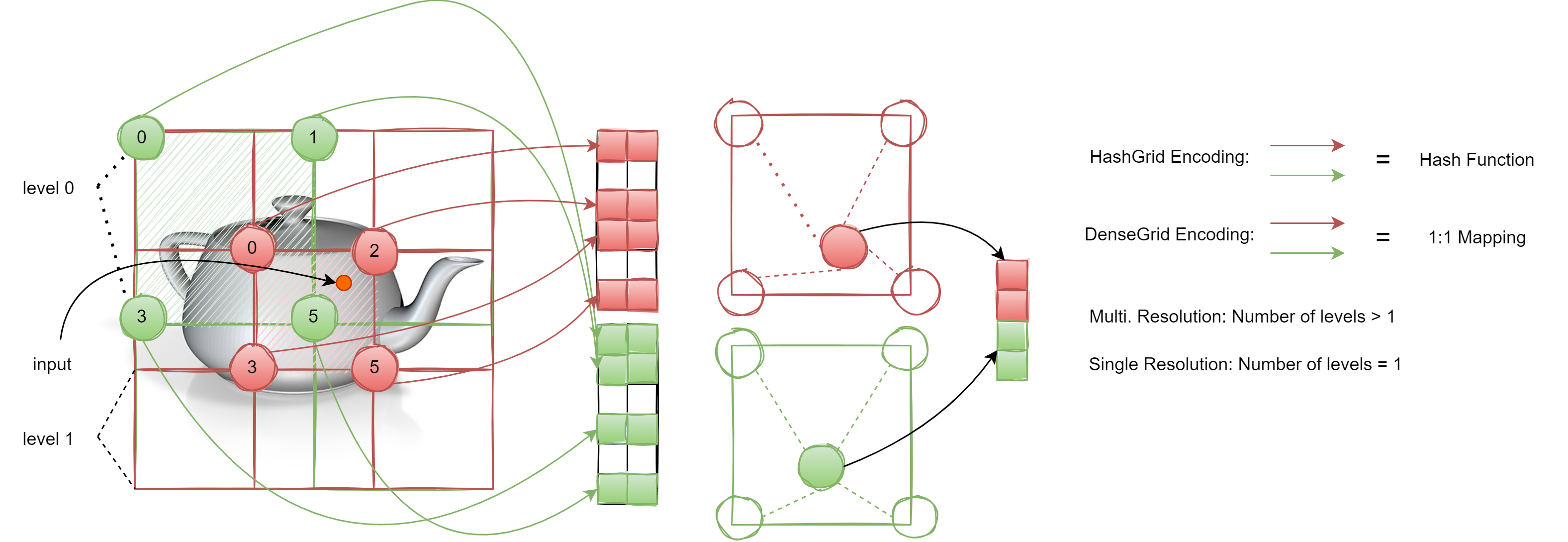
Figure 6: Illustration of Multi resolution grid encoding.

The different steps performed in multi-resolution grid encoding are explained in Figure 6. The encoding parameters are arranged into L levels, each containing up to T feature vectors with dimensionality F. Each level is independent and stores the feature vectors at the vertices of a grid. Each corner of the grid is mapped to an entry in the level’s respective feature vector array where each feature vector array has a fixed size of T. The mapping between the grid and the feature vector array is 1:1 for coarse levels because the dense grid requires fewer than T parameters for coarse levels. However, for finer levels, the feature vector can either be mapped 1:1 or treated as hash table and a hash function can be used to index into the array [17]. The input encoding, where a hash function is used to index into lookup table, is called multi-resolution hashgrid encoding. Whereas, the encoding where 1:1 mapping is used for all the resolution levels is known as multi-resolution densegrid encoding. The hash function used by the state of the art parametric encoding scheme (instant-NGP [17]) is presented in Equation 1.

$$h(x)=(\oplus_{i=1}^{d}x_{i}\pi_{i})~{}mod~{}T$$ (1)

where $\oplus$ denotes the bit-wise XOR operation and $\pi$ are unique large prime numbers. The feature vectors at each corner of the grid are linearly interpolated to ensure continuous representation. The interpolated feature vectors for all the levels are then concatenated to generate the final encoded input to the multi-layer perceptron, as shown in Figure 6. The number of training parameters are bounded by $T\times L\times F$.  [17] has shown that for multi-resolution hashgrid encoding only using 16 levels and 2 features per array entry produces high fidelity image frames for many neural graphics applications, hence the number of trainable encoding parameters is set $T\times 16\times 2$ where T ranges from $2^{14}~{}to~{}2^{24}$ depending upon the neural graphics application and the desired image fidelity. For multi-resolution densegrid encoding 2-8 levels can be used to get high visual fidelity outputs.

III Does Neural Graphics Need Hardware Support?

To understand the performance characteristics of neural graphics, we focus on the following four representative neural graphics applications that cover a relatively wide range of graphics tasks, as presented by Müller et al. [19], including rendering, novel view synthesis, 3D shape representation, simulation, path planning, 3D modeling and image approximations:

1) Neural radiance and density fields (NeRF): The learning objective during training phase is is to learn the 3D density and the 5D light field of a given scene from a few scene observations (images or video of the scene). The structure of the NeRF application is shown in Figure 4. In NeRF, two fully-connected neural networks, 1) Density MLP and 2) Color MLP, are concatenated together where density MLP learns the density information $(\sigma)$ and the color MLP learns the view dependent $(RGB)$ color information of the scene. As the density information of a scene is view direction agnostic, the encoded coordinates/positions $(x,y,z)$ are used as input to the density MLP. As the color information depends upon position as well as view angle, the output of the density MLP along with the encoded view directions $(\theta,\phi)$ are passed as input to the color MLP. The output of the color MLP is a three dimensional vector containing the pixel color information $(RGB)$. The density information is then concatenated with the pixel color information to get the four dimensional vector containing the pixel color and the density information $(RGB,\sigma)$.

2) Neural signed distance functions (NSDF): In classical computer graphics, signed distance functions (SDFs) are used to represent a 3D shape as the zero level-set of a function of position x. In graphics, SDFs are commonly used in applications such as simulation, path planning, 3D modeling, and video games [17]. In neural approximations of SDFs, the MLP learns the mapping from 3D coordinates to the distance to a surface. The structure of the NSDF application is shown in Figure 4. The inputs to the MLP are encoded positions and the final output is the distance to the surface.

3) Gigapixel image approximation (GIA): A gigapixel image is an ultra high definition digital image bitmap, usually made by combining multiple detailed images into a single image. A Gigapixel image has billions of pixels, which is much more than the capacity of a normal professional camera. In GIA a neural network is used to approximately learn the gigapixel image in its trainable parameters. The learning objective of the MLP in GIA application is to learn the mapping from 2D coordinates to RGB colors of the gigapixel image. The structure of the GIA application is shown in Figure 4. As the MLP learns the 2D image, there is no density information and hence the view direction is also not required; the inputs to the MLP are the encoded pixel positions and the outputs are the corresponding pixel color $(RGB)$. This application can be considered as an important benchmark to test neural network’s ability to learn the high frequency details of visual data.

4) Neural volume renderer (NVR): This application is similar to NeRF. The only difference is that, instead of learning the density and the emission field, the network in neural volume rendering learns the density and a reflectance field, which can be used to simulate the light transport in the volume using path tracing. The structure of the NVR application is shown in Figure 4. In NVR, two fully-connected neural networks, 1) Density MLP and 2) Color MLP, are concatenated together where the density MLP learns the density information $(\sigma)$ and the color MLP learns the view dependent $(RGB)$ color information of the bounded object. Similar to NeRF, the encoded positions $(x,y,z)$ are used as input to the density MLP and the output of the density MLP along with the encoded view directions $(\theta,\phi)$ are passed as input to the color MLP. The output is a four dimensional vector containing the pixel color and the density information $(RGB,\sigma)$.

Each application can be implemented using a variety of input encodings. As parametric encodings produce strictly better output fidelity than frequency encodings [17, 19, 6, 10], we picked parametric encoding for further exploration. In order to faithfully represent the state of the art in parametric encodings, we explored three different types of parametric encodings in this work – 1) Multi resolution hashgrid encoding: Hash function is used to generate the indices of the lookup tables while mapping the grid features to the lookup tables entries. The number of resolution levels used is 16 [17, 18]. 2) Multi resolution densegrid encoding: 1:1 mapping is used between grid features and the lookup tables entries. The number of resolution levels used is 8 [17, 18] 3) Low resolution densegrid encoding: 1:1 mapping is used between grid features and the lookup tables entries. The number of resolution levels used is 2 [17, 18]

We profiled the above four neural graphics applications with the chosen three input encoding schemes using the open source code published by Müller et al [18]. The parameters for all our neural graphics applications and encoding schemes are shown in Table I. Both the input encoding algorithm and the multi-layer perceptron are implemented as separate fused CUDA kernels [19, 18, 17]. Unlike standard MLPs the fully-fused MLPs do not have any explicit biases. Due to the smaller size of the fully-fused MLPs, the intermediate activations and the partial sums can be stored on the faster on-chip memory, reducing the number of global memory accesses. A python based wrapper generates the inputs and displays the final rendered frame. We run the applications on Nvidia’s RTX3090 using CUDA version 11.7 and report the total runtime of the applications.

Our results (Figure 5) show that, on a modern desktop class GPU (RTX3090), for multi resolution hashgrid encoding, rendering $\sim 2M$ pixels ($1920\times 1080$ frame) takes $231msec$, $27.87msec$, $2.12msec$ and $6.32msec$ for NeRF, NSDF, GIA and NVR respectively. This is unacceptable for real-time applications. For instance, if we want to render 4k frames at 60FPS only one of our neural graphics applications (GIA) is able to meet that target, there is the performance gap of $55.50\times$, $6.68\times$, and $1.51\times$ for NeRF, NSDF and NVR respectively.

In order to understand the performance bottlenecks of neural graphics applications, we perform kernel level performance breakdown analysis. Figure 5 shows that input encoding and multi-layer perceptron are the two most expensive kernels in all neural graphics applications. For multi resolution hashgrid encoding, on average across all neural graphics applications, $40.24\%$ of the total number of cycles are consumed by the input encoding kernel and $32.12\%$ cycles are consumed by the multi-layer perceptron kernel. On average, this amounts to $72.37\%$ of application time. For multi resolution densegrid encoding, on average across all neural graphics applications, $24.63\%$ of the total number of cycles are consumed by the input encoding kernel and $35.37\%$ cycles are consumed by the multi-layer perceptron kernel. On average, this amounts to $60.0\%$ of application time. For low resolution densegrid encoding, on average across all neural graphics applications, $24.15\%$ of the total number of cycles are consumed by the input encoding kernel and $35.37\%$ cycles are consumed by the multi-layer perceptron kernel. On average, this amounts to $59.96\%$ of application time. This data motivates the need to accelerate the input encoding and multi-layer perceptron kernels. In next section, we will provide a further breakdown of the time spent in the input encoding and the multi-layer perceptron kernels to understand their performance bottlenecks.

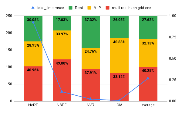
(a)

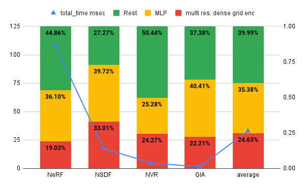
(b)

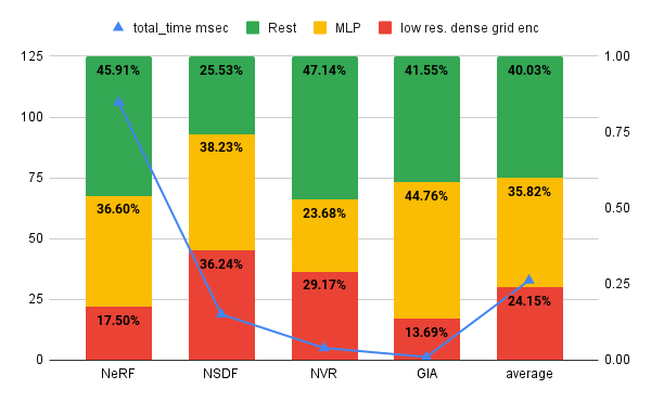
(c)

Figure 5: Kernel level performance breakdown analysis of neural graphics applications: The number of cycles consumed by the different kernels of the neural graphics applications (as percentage of total application cycles). (a) Multi resolution hashgrid encoding, (b) Multi resolution densegrid encoding, (c) Low resolution densegrid encoding.

IV Understanding Performance of Neural Graphics Applications

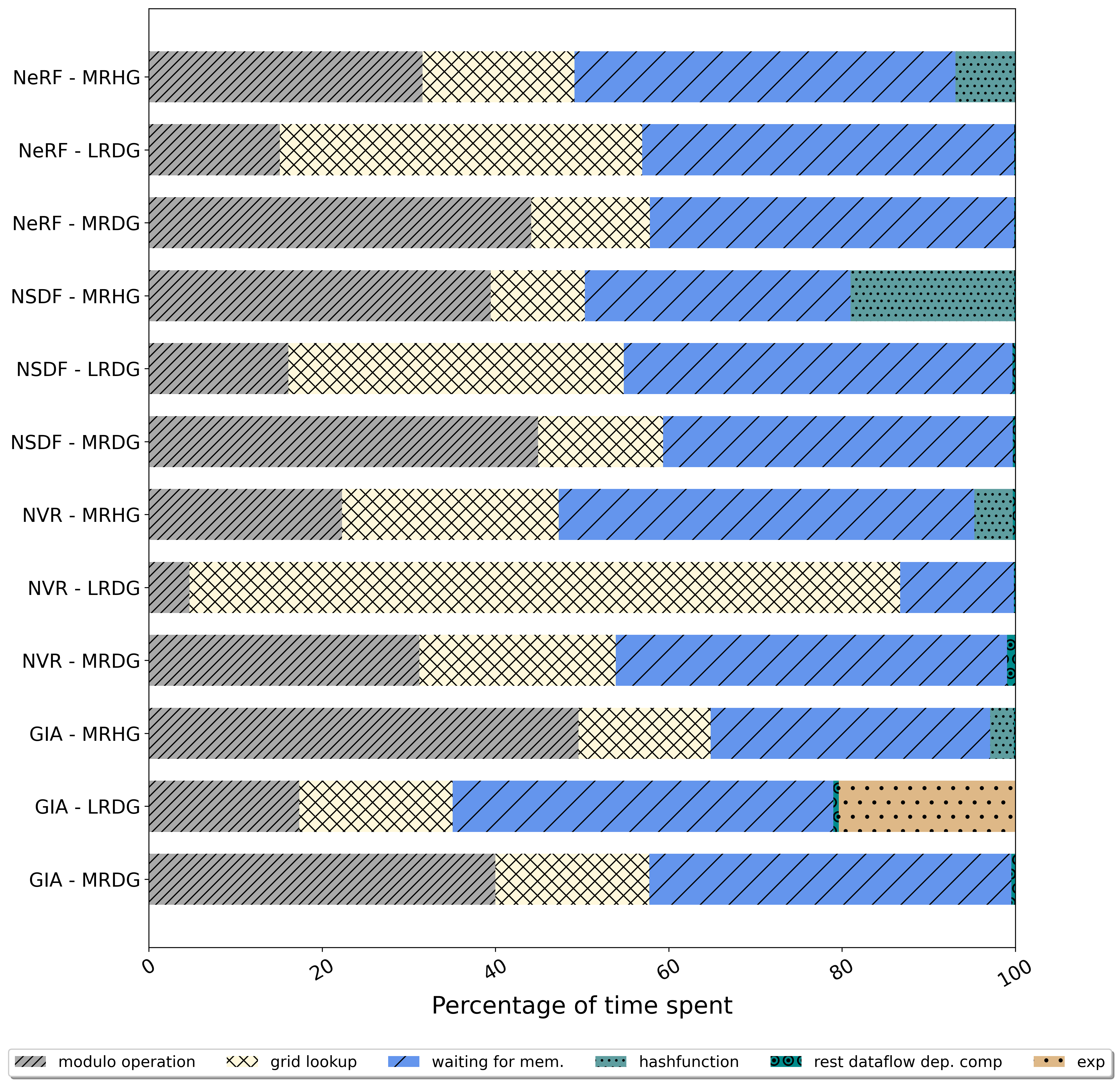
Figure 8: The operation level breakdown of the of input encoding kernels for different input encoding types. The five most expensive operations in terms of number of cycles spent. MRHG : multi resolution hashgrid , MRDG : multi resolution densegrid , LRDG : low resolution densegrid .

We performed further analysis (using Nvidia’s nsight compute) to understand the performance bottlenecks in the input encoding and multi-layer perceptron kernels. Figure 8 shows the operation level breakdown of the of input encoding kernels for different input encoding types. Five most expensive operations in terms of number of cycles spent are labeled in the Figure 8. As explained in Section II, the grid lookups are the major building block of the input encoding algorithms; our analysis also shows that the grid lookups take significant amount of cycles across all three input encoding types.

The percentage utilization of the GPU compute and memory resources, for the input encoding kernel is presented in Table II. On average, across all encoding kernel calls, the memory utilization of the GPU is higher than compute utilization. This is because input encoding is a memory intensive workload that requires performing lookup operations for mapping inputs to learned features even as the lookup tables for all the resolution levels do not entirely fit on the L2 cache of RTX3090. The memory wait time to resolve the cache misses also adds to the overall cycles. Our analysis also shows that the integer mapped modulo operation is one of the most expensive operations for all three input encoding types. This is because the modulo operation gets mapped to the less efficient general integer modulo operation instead of using more efficient bitwise operations which account for the fact that hash map sizes are always powers of two.

As multi resolution densegrid and low resolution densegrid have one-on-one mapping of grid indices, the hash function is not called for these input encoding types and hence the breakdown shows zero cycles for the hash function. However, the hash function consumes significant number of cycles for multi resolution hashgrid . This is because the hash function cannot efficiently utilize the ALU due to the stalls caused by waiting on the long scoreboard to resolve the global memory requests. As shown in the input encoding breakdown (Figure 8), other relatively simple compute operations also consume significant number of cycles because they have to wait for the long scoreboard to resolve the global memory requests corresponding to the grid lookups.

Table II also presents the the percentage utilization of the GPU compute and memory resources for the MLP kernel. Our results show that for MLP kernels as well, the memory utilization is higher than compute utilization. This is because, for a constant batch size, the compute cost of the fully connected networks scales quadratically with the width of the network (Compute Cost: $O(M^{2})$) whereas the memory traffic scales linearly (Memory Cost: $O(M)$). For relatively big MLPs with a large number of neurons, the quadratic compute cost quickly becomes the bottleneck and further optimizing memory traffic has little to no performance benefits because the cost would be overshadowed by the quadratic compute requirements. However, all our neural graphics applications have tiny MLPs, with only 2-4 hidden layers and 64 hidden neurons per layer (Table I). In smaller MLPs, the compute cost and the linear memory traffic become asymptotically comparable and hence the memory traffic cost starts to matter. Moreover, the GPUs and the modern processors in general usually have larger computational throughput than memory bandwidth, which means that, for small number of neurons, the memory cost dominates.

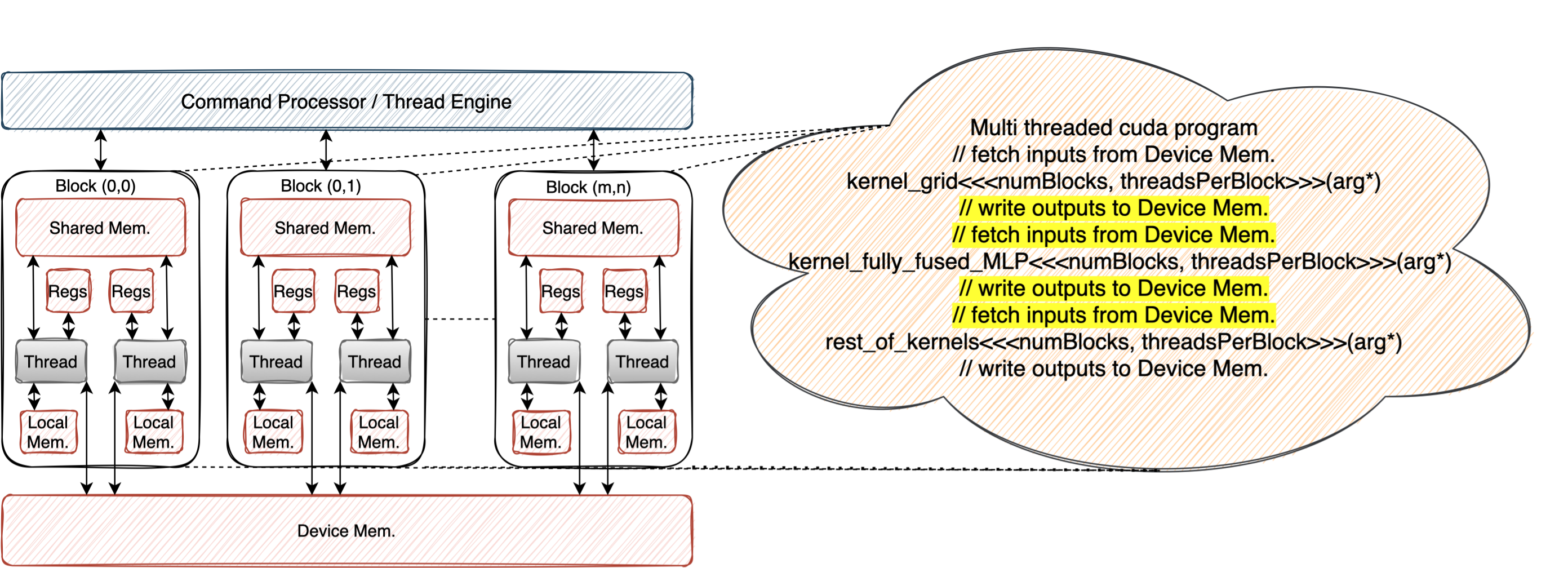
Figure 7: Scheduling of a typical neural graphics application on GPU.

TABLE I: The parameters of the four neural graphics applications for different input encoding schemes.

Application	Parameters
NeRF multi res. hashgrid	GridEncoding: Nmin=16 b=1.51572 F=2 T=2^19 L=16 Density model: 3–[HashGrid]–>32–[FullyFusedMLP(neurons=64;layers=3)]–>1 Color model: 3–[Composite]–>16+16–[FullyFusedMLP(neurons=64;layers=4)]–>3
NeRF multi res. densegrid	GridEncoding: Nmin=16 b=1.405 F=2 T=2^19 L=8 Density model: 3–[DenseGrid]–>16–[FullyFusedMLP(neurons=64;layers=3)]–>1 Color model: 3–[Composite]–>16+16–[FullyFusedMLP(neurons=64;layers=4)]–>3
NeRF low res. densegrid	GridEncoding: Nmin=128 b=1 F=8 T=2^19 L=2 Density model: 3–[TiledGrid]–>16–[FullyFusedMLP(neurons=64;layers=3)]–>1 Color model: 3–[Composite]–>16+16–[FullyFusedMLP(neurons=64;layers=4)]–>3
NSDF multi res. hashgrid	GridEncoding: Nmin=16 b=1.38191 F=2 T=2^19 L=16 Model: 3–[HashGrid]–>32–[FullyFusedMLP(neurons=64;layers=4)]–>1
NSDF multi res. densegrid	GridEncoding: Nmin=16 b=1.405 F=2 T=2^19 L=8 Model: 3–[DenseGrid]–>16–[FullyFusedMLP(neurons=64;layers=4)]–>1
NSDF low res. densegrid	GridEncoding: Nmin=128 b=1 F=8 T=2^19 L=2 Model: 3–[TiledGrid]–>16–[FullyFusedMLP(neurons=64;layers=4)]–>1
NVR multi res. hashgrid	GridEncoding: Nmin=16 b=1.275 F=2 T=2^19 L=16 Model: 3–[HashGrid]–>32–[FullyFusedMLP(neurons=64;layers=4)]–>4
NVR multi res. densegrid	GridEncoding: Nmin=16 b=1.405 F=2 T=2^19 L=8 Model: 3–[DenseGrid]–>16–[FullyFusedMLP(neurons=64;layers=4)]–>4
NVR low res. densegrid	GridEncoding: Nmin=128 b=1 F=8 T=2^19 L=2 Model: 3–[TiledGrid]–>16–[FullyFusedMLP(neurons=64;layers=4)]–>4
GIA multi res. hashgrid	GridEncoding: Nmin=16 b=1.25992 F=2 T=2^24 L=16 Model: 2–[HashGrid]–>32–[FullyFusedMLP(neurons=64;layers=4)]–>3
GIA multi res. densegrid	GridEncoding: Nmin=16 b=1.405 F=2 T=2^24 L=8 Model: 2–[DenseGrid]–>16–[FullyFusedMLP(neurons=64;layers=4)]–>3
GIA low res. densegrid	GridEncoding: Nmin=128 b=1 F=8 T=2^24 L=2 Model: 2–[TiledGrid]–>16–[FullyFusedMLP(neurons=64;layers=4)]–>3

TABLE II: The percentage utilization of the GPU compute and memory resources, for the input encoding and the MLP kernels for all four neural graphics applications and for different input encodings.

App.-Kernel	Grid Size/Block Size	Comp. Util. per kernel call	Mem. Util. per kernel call	Kernel Calls	Comp. Util. avg. across application	Mem. Util. avg. across application
NeRF multi res. hashgrid	(3853;16;1)/(512;1;1)	61.73	72.85	59	40.63	72.02
NeRF MLP	(3853;16;1)/(512;1;1)	34.3	65.2	118	33.36	63.07
NSDF multi res. hashgrid	(1823;16;1)/(512;1;1)	73.08	43.54	256	15.97	30.8
NSDF MLP	(1823;16;1)/(512;1;1)	38.13	71.74	256	9.76	18.28
NVR multi res. hashgrid	(403;16;1)/(512;1;1)	52.5	59.03	48	18.67	30.36
NVR MLP	(403;16;1)/(512;1;1)	36.51	67.01	48	11.51	21.05
GIA multi res. hashgrid	(4050;16;1)/(512;1;1)	82.87	62.23	1	82.87	62.23
GIA MLP	(4050;16;1)/(512;1;1)	39.1	72.22	1	39.1	72.22
NeRF multi res. densegrid	(3966;8;1)/(512;1;1)	71.39	91.81	45	57.37	72.31
NeRF MLP	(3966;8;1)/(512;1;1)	39.53	68.4	90	34.51	62.31
NSDF multi res. densegrid	(1823;8;1)/(512;1;1)	76.1	48.25	244	18.38	21.28
NSDF MLP	(1823;8;1)/(512;1;1)	41.66	73.49	244	11.06	19.41
NVR multi res. densegrid	(403;8;1)/(512;1;1)	57.38	56.8	48	17.41	22.43
NVR MLP	(403;8;1)/(512;1;1)	39.83	67.67	48	12.17	20.59
GIA multi res. densegrid	(4050;8;1)/(512;1;1)	78.53	65.83	1	78.53	65.83
GIA MLP	(4050;8;1)/(512;1;1)	42.89	73.07	1	42.89	73.07
NeRF low res. densegrid	(3980;2;1)/(512;1;1)	53.83	49.74	43	31.17	59.57
NeRF MLP	(3980;2;1)/(512;1;1)	39.41	68.17	86	35.5	64.1
NSDF low res. densegrid	(1823;2;1)/(512;1;1)	55.88	45.52	260	7.21	20.07
NSDF MLP	(1823;2;1)/(512;1;1)	41.37	72.98	260	10.34	18.14
NVR low res. densegrid	(403;2;1)/(512;1;1)	22.71	69.16	48	6.29	22.71
NVR MLP	(403;2;1)/(512;1;1)	39.2	66.58	48	12.11	20.48
GIA low res. densegrid	(4050;2;1)/(512;1;1)	66.15	59.12	1	66.15	59.12
GIA MLP	(4050;2;1)/(512;1;1)	42.87	73.02	1	42.87	73.02

V Neural Fields Processor: An Architecture for Neural Graphics

Since our profiling motivates the need to accelerate the input encoding and multi-layer perceptron kernels, we design an architecture - a neural fields processor  (Figure 9) - to accelerate the input encoding and multi-layer perceptron kernels in hardware using separate hardware engines for the two. To accelerate input encoding kernel, our kernel level analysis (Section IV) suggests providing hardware support for the grid lookups and the dataflow of the input encoding. Moreover, in neural graphics applications, the outputs of the input encoding kernel are always consumed by the multi-layer perceptron kernel (Figure  4) In Müller et al’s GPU implementation of these applications [18, 17], the input encoding kernel writes outputs to device memory and the multi-layer perceptron kernel fetches that data again for further processing (Figure 7). This leads to unnecessary memory traffic and waste of energy for DRAM accesses that can potentially be avoided. This opportunity can be exploited in the neural fields processor hardware by fusing the input encoding and multi-layer perceptron engines in such a way that the input encoding engine directly writes the outputs to the input memory of the multi-layer perceptron engine.

Figure 9-a presents the architecture of the input encoding hardware engine. Each input encoding hardware engine has a dedicated on-chip SRAM (grid_sram) to cache the lookup table for one resolution level. The size of the grid_sram (1MB per input encoding engine) is chosen such that the entire lookup table for one resolution level fits on the on-chip SRAM, and the off-chip memory access penalty could be avoided for grid lookups. The lookup table for one resolution level is cached once on the dedicated grid_sram of one input encoding engine and then lookups are performed for all the inputs for the entire frame. Our hardware architecture has 16 input encoding engines to match the maximum number of resolution levels of the neural graphics applications. As the multi resolution hashgrid input encoding has 16 resolution levels, each of the 16 input encoding engines caches the lookup table corresponding to one resolution level and then performs the input encoding for all the resolution levels in parallel. As multi resolution densegrid input encoding has 8 resolution levels, two inputs can be processed in parallel. Similarly, as low resolution densegrid input encoding has 2 resolution levels, the input encoding IP can process 8 inputs in parallel.

The normalized input coordinates are pre-fetched into the input FIFO (Figure 9-a). The grid_scale module calculates the scale of the grid from the base-resolution of the grid and the resolution level being processed. The pos_fract module is responsible for converting the normalized input coordinates to the absolute coordinates. It multiplies the normalized coordinates with grid scale to compute the absolute coordinates, which are then passed to the grid_index module for the index calculation. The grid_index module is responsible for calculating the final indices for the lookup operations. The grid_index module can be configured to either hash in the indices for the multi resolution hashgrid encoding or compute the indices without the hashing function for the multi resolution densegrid and low resolution densegrid encoding types. The algorithm to compute the indices for the lookup operation takes the modulo of the indices with the hash-map size as an intermediate operation before the final indices could be calculated. We observe that the hash-map size is always power of two for all our neural graphics applications. We exploit this optimization opportunity in hardware and approximate the modulo operation with shift operation in input encoding engine. The final outputs of the grid_index modules are actual indices that are directly used to perform the feature lookups from the grid_sram. The interpol_weights module computes the interpolation weights that are then multiplied with the features to compute the final features that are fed to the multi-layer perceptron engine. As each input encoding engine calculates features for one resolution level, the outputs of the input encoding engines are concatenated together to get the final input vector for the MLP engine.

Since MLPs in neural graphics applications are small (2-4 hidden layers, 64 neurons in each hidden layer), our MLP engine has a $64\times 64$ grid of MAC units that computes one layer of the multi-layer perceptron at a time. As the size of the hidden layer is relatively small, a dedicated small on-chip SRAM is used to store the intermediate features of the hidden layers. Keeping the intermediate features on-chip removes the off-chip memory accesses for storing/fetching the intermediate features and improves the performance by 1OOM  [19].

Figure 10-a shows the interaction of the neural fields processor with the GPU. A set of N NFPs are organized as a neural graphics processing cluster (NGPC) connected to the shared L2 cache. Figure 10-b and 10-c show the programming model of the NGPC. The programming model for the NGPC involves the GPU command buffer [8] configuring the NGPC and scheduling the input encoding and the multi-layer perceptron kernels on the NGPC. The rest of the kernels are scheduled just as conventional CUDA kernels on the streaming multiprocessors. The outputs of the NGPC are written back to the GPU memory, and are read by the streaming multiprocessors, which then compute the rest of the kernels. The inputs are divided into batches. While the GPU is processing the rest of the neural graphics application kernels for the Nth batch of inputs, the N+1st batch is scheduled on the NGPC to compute the input encoding and MLP kernels in parallel, as shown in Figure 10-b.

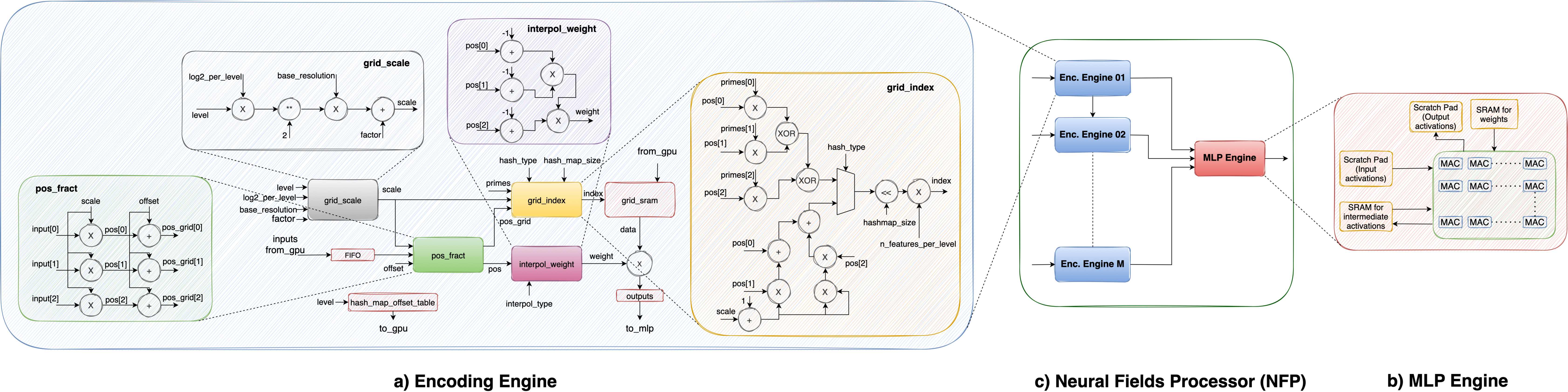
Figure 9: Architecture of the Neural Fields Processor (NFP)

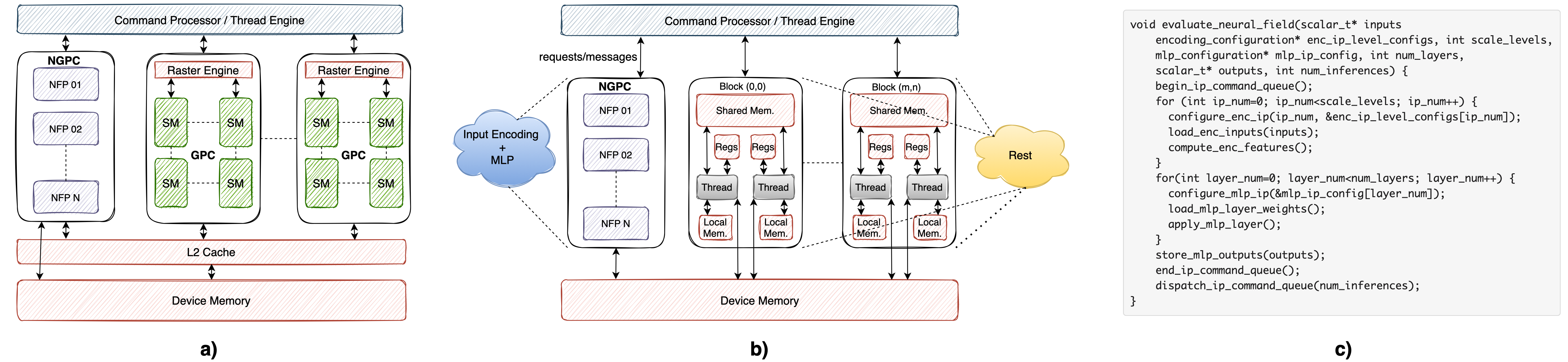
Figure 10: a) Interaction of the NGPC with GPU. b) Programming model for NGPC. c) Pseudocode for programming NGPC.

VI Evaluation and Results

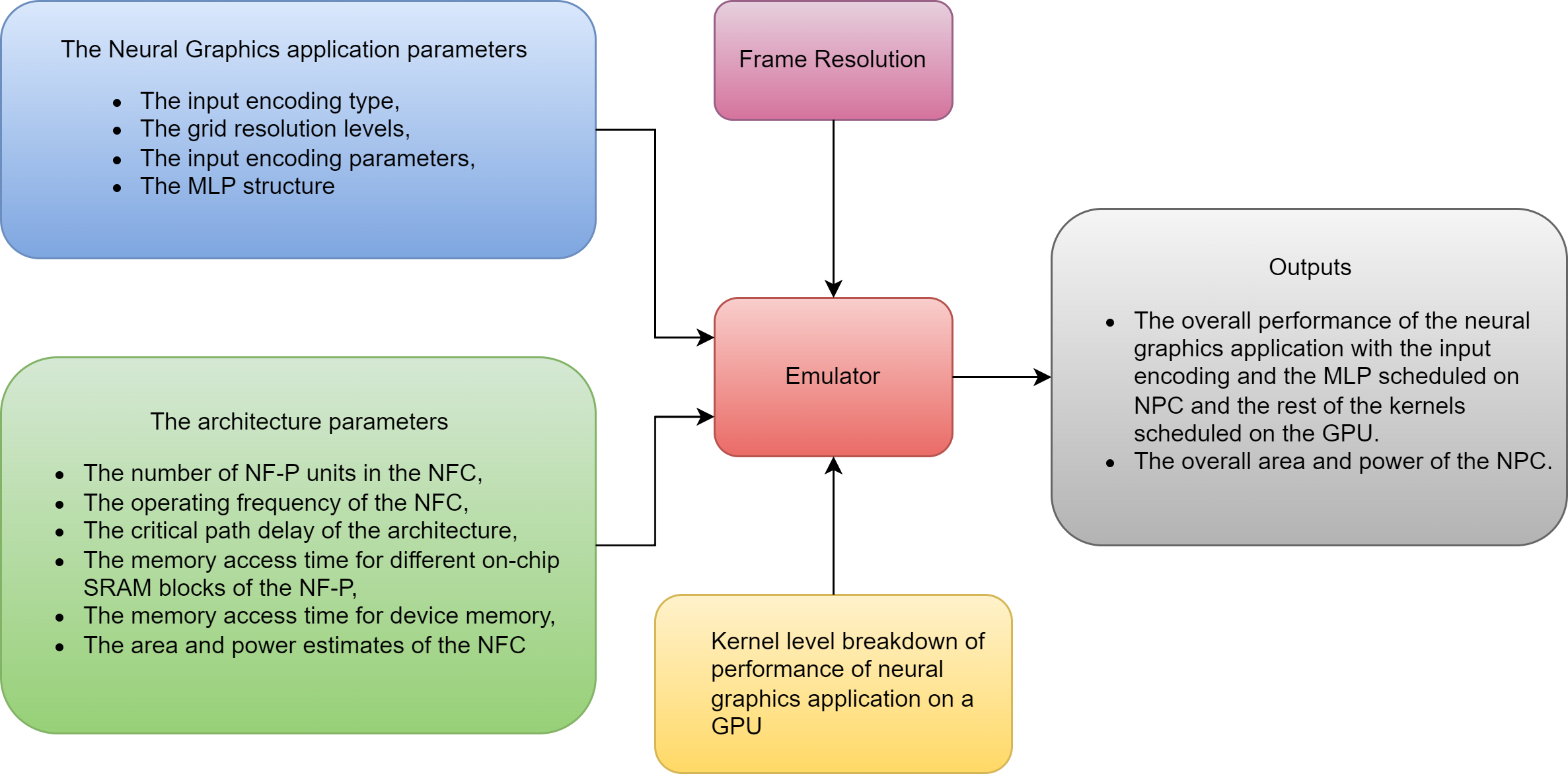
Figure 11: Block diagram of the emulator.

We provide an emulator to evaluate the performance of the neural graphics applications on our architecture. The block diagram of the emulator is in Figure 11. The inputs to the emulator are 1) The neural graphics application parameters such as the input encoding type, the grid resolution levels, the input encoding parameters, the multi-layer perceptron structure 2) the architecture parameters such as the number of NFP units in the NGPC, operating frequency of the NGPC, the critical path delay of the architecture, the memory access time for different on-chip SRAM blocks of the NFP , the memory access time for device memory, the area and power estimates of the NGPC 3) the kernel level breakdown of the performance of the neural graphics application on the GPU and 4) the frame resolution. The outputs of the emulator are 1) the overall performance of the neural graphics application with the input encoding and the multi-layer perceptron scheduled on NGPC and the rest of the kernels scheduled on the GPU. 2) the overall area and power of the NGPC.

We evaluated the performance of the neural graphics applications on our proposed architecture for the scaling factor of 8, 16, 32 and 64, where NGPC-8 has 8 NFP unit, NGPC-16 has 16 NFP units and so on. Figure 12a presents the overall performance of the neural graphics applications with multi resolution hashgrid encoding on the proposed architecture. Our results show that when we have only 8 NFP units in the NGPC, on average across all four neural graphics applications, we get overall $12.94\times$ performance benefits compared to the GPU baseline. When we scale the number of NFP units in an NGPC to 16, 32 and 64, the performance benefits averaged across the four representative neural graphics applications increase to $20.85\times$, $33.73\times$ and $39.04\times$ respectively.

Figure 12b presents the overall performance of the neural graphics applications with multi resolution densegrid encoding. Our results show that when we have only 8 NFP units in NGPC, on average across all four neural graphics applications, we get overall $9.05\times$ performance benefits compared to the GPU baseline. When we scale the number of NFP units in an NGPC to 16, 32 and 64, the performance benefits averaged across the four representative neural graphics applications increase to $14.22\times$, $22.57\times$ and $26.22\times$ respectively.

Figure 12c presents the overall performance of the neural graphics applications with low resolution densegrid encoding. Our results show that when we have only 8 NFP units in NGPC, on average across all four neural graphics applications, we get overall $9.37\times$ performance benefits compared to the GPU baseline. When we scale the number of NFP units in an NGPC to 16, 32 and 64, the performance benefits averaged across the four representative neural graphics applications increase to $14.66\times$, $22.97\times$ and $26.4\times$ respectively.

Our results also show that NeRF performance plateaus for NGPC-64. I.e., increasing the number of NFP beyond 64 does not improve the overall performance of the application. This is because the time consumed by the non- input encoding and multi-layer perceptron kernels becomes the performance bottleneck. Similarly, for NSDF , NVR and GIA the performance plateaus for NGPC-32, NGPC-16 and NGPC-64 respectively.

In order to better understand where the application level benefits are coming from, we also compare the performance of the input encoding and the multi-layer perceptron kernels individually, with their GPU based implementations. Figure 13 presents the performance improvement of the input encoding kernel and the multi-layer perceptron kernels individually, on our architecture, for scaling factors of 8, 16, 32 and 64. Our results show that for multi resolution hashgrid , on average across four neural graphics applications, the neural graphics processing cluster -64 has performance improvement of $246\times$ and $1232\times$ for the input encoding kernel and the multi-layer perceptron kernel, respectively. For multi resolution densegrid , neural graphics processing cluster -64 has performance improvement of $379\times$ and $1070\times$ for the input encoding kernel and the multi-layer perceptron kernel, respectively. For low resolution densegrid , the neural graphics processing cluster -64 has performance improvement of $2353\times$ and $1451\times$ for the input encoding kernel and the multi-layer perceptron kernel, respectively.

In Figure 14, we present the number of pixels that can be rendered for a given FPS target with and without neural graphics processing cluster . Horizontal lines in the figure mark the number of pixels in HD ($1280\times 720$), FHD ($1920\times 1080$), QHD/2k ($2560\times 1440$), Ultra HD/4k ($3820\times 2160$), 5k ($5120\times 2880$) and 8k ($7680\times 4320$) frame resolutions. The vertical bars show the number of pixels rendered within the time budget of 1000/30 = 33.33ms, 1000/60 = 16.67ms, 1000/90 = 11.11ms and 1000/120 = 8.33ms corresponding to the FPS targets of 30, 60, 90 and 120 FPS respectively. Our results show that with multi resolution hashgrid encoding, NGPC enables the rendering of 4k Ultra HD resolution frames at 30 FPS for NeRF and 8k Ultra HD resolution frames at 120 FPS for all our other neural graphics applications.

For estimating the area and power overheads, we wrote RTL for neural fields processor and synthesized it using Synopsys design compiler along with the Nangate 45nm open cell library. We used CACTI to get the area and power estimates for the SRAM blocks. Figure 15 shows the area and power of the different configurations of NGPC normalized with respect to Nvidia’s RTX3090 area and power. In order to get iso-technode comparison, we scaled the area and power of NGPC to 7nm using often-used scaling formulas [31]. Our estimates show that NGPC-8 that has only one NFP unit increases the die area of GPU by only $\sim 4.52\%$ with the power overhead of $\sim 2.75\%$. Similarly, NGPC-16, NGPC-32 and NGPC-64 increase the GPU die area by $\sim 9.04\%$, $\sim 18.01\%$ and $\sim 36.18\%$ respectively and GPU power by $\sim 5.51\%$, $\sim 11.03\%$ and $\sim 22.06\%$ respectively.

Table III presents the input/output bandwidth and the data access time for our NGPC architecture. Our estimates suggest that, for 60FPS, the bandwidth requirement for NGPC architecture is 231 GB/s for NeRF and 69 GB/s for all other neural graphics applications. The memory bandwidth of Nvidia RTX 3090 is 936.2 GB/s  [1]. Hence, for 60FPS, the IO bandwidth of the accelerator is $\sim 24\%$ of the GPU memory bandwidth for NeRF and only $\sim 7\%$ of the GPU memory bandwidth for NSDF, NVR and GIA. Moreover, the massively parallel nature of the workload and the high memory bandwidth of the GPU compared to the IO bandwidth of the accelerator keeps the encoding engines busy with high utilization. This translates to data access time of 4.12ms for NeRF and 1.23ms for all other neural graphics applications.

In order to get confidence in our evaluation methodology and the reported speedup numbers, we performed a sanity check against Amdahl’s law and presented our analysis in figures 12a, 12b and 12c. Horizontal lines in the figures 12a, 12b and 12c show the peak speedup bounded by Amdahl’s law and the vertical bars show the reported speedup from our emulator. Our analysis shows that the reported speedup is always under the Amdahl-driven analytical bounding of speedup. We also modeled the performance of our MLP engine using popular open-source DNN-architecture-modeling frameworks Timeloop [23] and Accelergy [41]. In figure 13 we also present the performance benefits of the MLP engine modeled with the timeloop and accelergy. Our analysis shows that the performance benefits reported by our emulator are within $\sim 7\%$ of the the performance benefits modeled with the timeloop and accelergy.

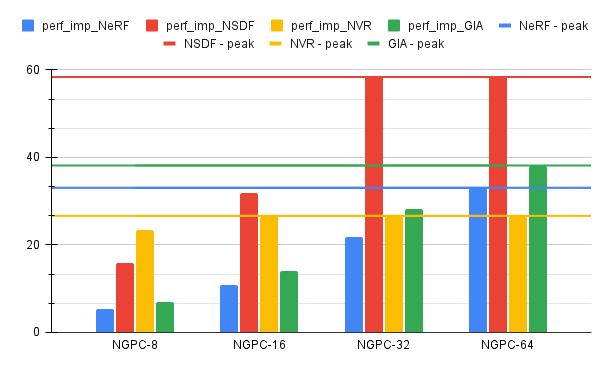
(a)

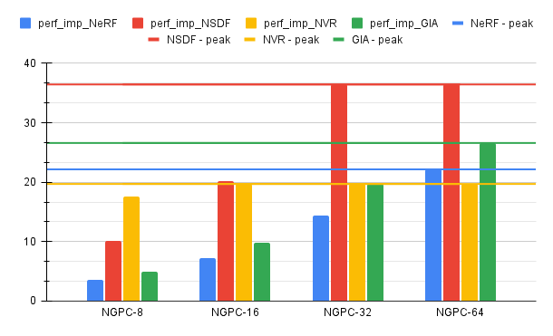
(b)

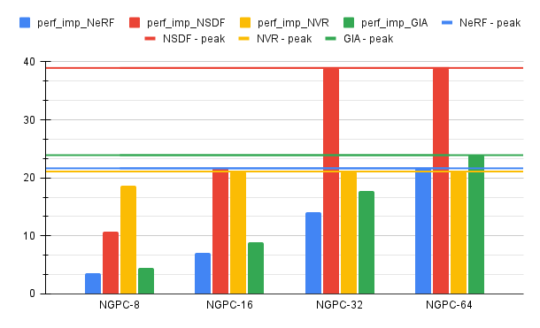
(c)

Figure 12: The performance of the neural graphics applications on our proposed architecture for the scaling factor of 8, 16, 32 and 64. NGPC-8 has 8 NFP units, NGPC-16 has 16 NFP units and so on. (a) Multi resolution hashgrid encoding, (b) Multi resolution densegrid encoding, (c) Low resolution densegrid encoding.

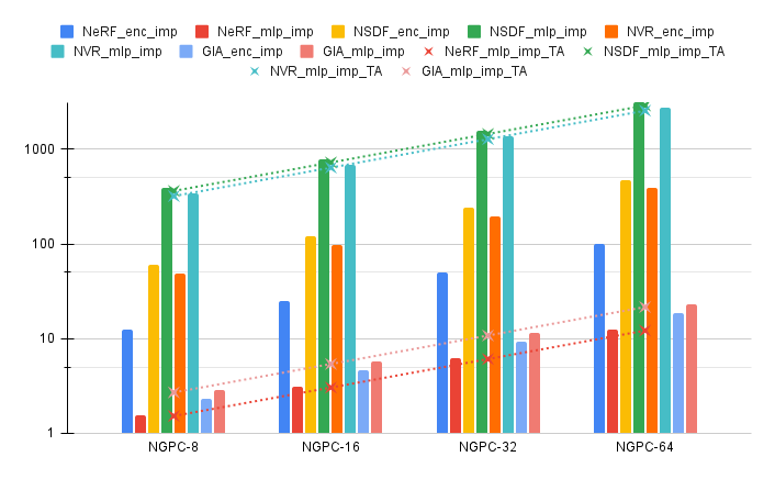
(a)

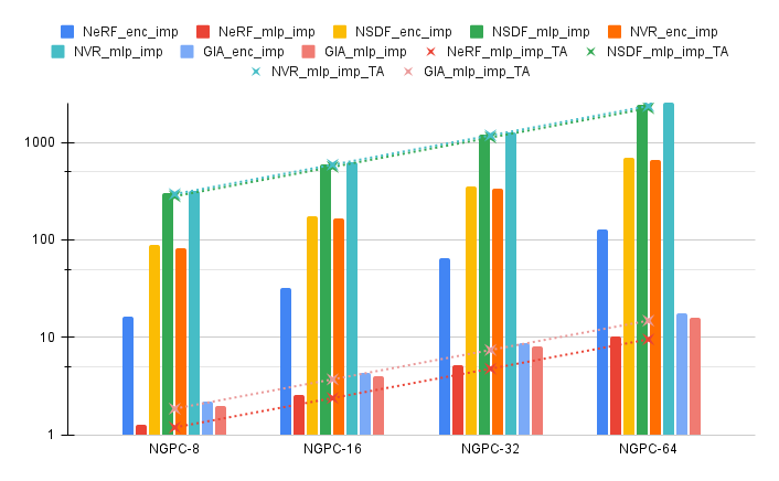
(b)

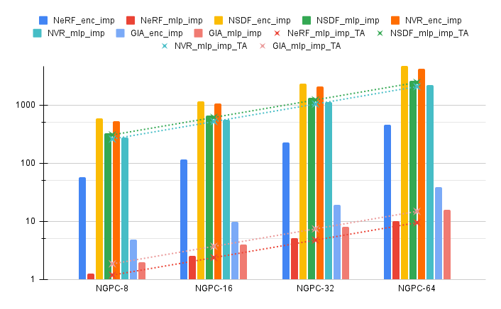
(c)

Figure 13: The performance improvement of the input encoding kernels and the multi-layer perceptron kernels individually, on our architecture, for the scaling factors of 8, 16, 32 and 64. For all four neural graphics applications and different input encoding types. (a) Multi resolution hashgrid encoding, (b) Multi resolution densegrid encoding, (c) Low resolution densegrid encoding, where dotted lines labeled as mlp_imp_TA are the performance improvements of MLP engine modeled with timeloop and accelergy.

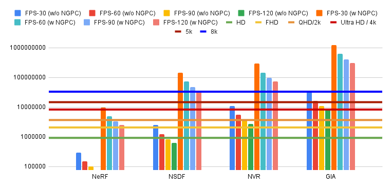
(a)

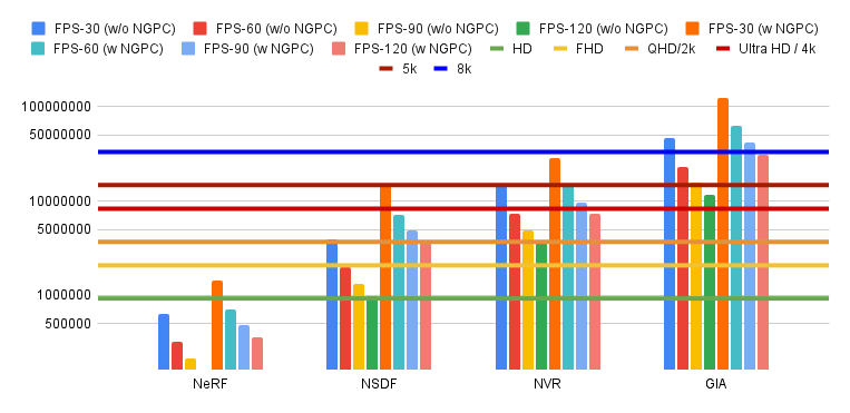
(b)

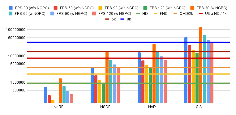
(c)

Figure 14: The number of pixels that can be rendered for a given FPS target with and without neural graphics processing cluster. (a) Multi resolution hashgrid encoding, (b) Multi resolution densegrid encoding, (c) Low resolution densegrid encoding.

TABLE III: The input/output bandwidth and the data access time for our NGPC architecture.

App.	Input BW (GB/s)	Output BW (GB/s)	Totoal BW (GB/s)	Access time (ms)
NeRF	69.523	46.349	231.743	4.126
NSDF	34.761	34.761	69.523	1.238
GIA	34.761	34.761	69.523	1.238
NVR	34.761	34.761	69.523	1.238

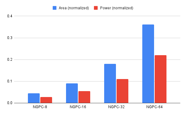
Figure 15: The area and Power of neural graphics processing cluster , normalized with respect to the area and power of Nvidia RTX 3090 die area and power.

VII Summary and Conclusion

Neural graphics promises a fast, deterministic time replacement for traditional rendering algorithms. In this paper, we address the question: does neural graphics need hardware support? We studied four representative neural graphics applications (NeRF, NSDF, NVR, and GIA) and showed that, if we want to render 4k resolution frames at 60FPS, there is the gap of $\sim 1.51\times$ to $55.50\times$ between the desired performance and the state of the art. For AR and VR applications, there is a larger gap of $\sim$ 2-4OOM between the desired performance and target power. Through in depth analysis, we identified that the input encoding and the multi-layer perceptron kernels are the performance bottlenecks consuming $72.37\%$, $60.0\%$ and $59.96\%$ of application time for multi resolution hashgrid encoding, multi resolution densegrid encoding and low resolution densegrid encoding respectively. Based on the compute and memory access characteristics of the input encoding and the multi-layer perceptron kernels, we proposed neural graphics processing cluster – a scalable hardware architecture that directly accelerates the input encoding and multi-layer perceptron kernels through dedicated engines and supports a wide range of neural graphics applications. To achieve good overall application level performance improvements, we also accelerate the rest of the kernels by fusion into a single kernel, leading to a $\sim 9.94\times$ speedup compared to previous optimized implementations [17] which is sufficient to remove this performance bottleneck. Our results show that, NGPC gives up to $58.36\times$ end-to-end application-level performance improvement. For multi resolution hashgrid encoding on average across the four neural graphics applications, the performance benefits of our architecture are $12.94\times$, $20.85\times$, $33.73\times$ and $39.04\times$ for the scaling factor of 8, 16, 32 and 64, respectively. For multi resolution densegrid encoding on average across the four neural graphics applications, the performance benefits of our architecture are $9.05\times$, $14.22\times$, $22.57\times$ and $26.22\times$ for the scaling factor of 8, 16, 32 and 64, respectively. Similarly, for low resolution densegrid encoding on average across the four neural graphics applications, the performance benefits of our architecture are $9.37\times$, $14.66\times$, $22.97\times$ and $26.4\times$ for the scaling factor of 8, 16, 32 and 64, respectively. Our results show that with multi resolution hashgrid encoding, NGPC enables the rendering of 4k Ultra HD resolution frames at 30 FPS for NeRF and 8k Ultra HD resolution frames at 120 FPS for all our other neural graphics applications.

VIII Acknowledgements

We thank Selvakumar Panneer (Intel) for multiple discussion about NeRF and neural graphics that helped conceive this project. We thank Anton Kaplanyan, Rama Harihara, Nilesh Jain, Ravi Iyer and Maxim Kazakov (from Intel) for multiple discussions about neural graphics. We also thank Vikram Sharma Mailthody, the anonymous reviewers as well as the members of the Passat group for their feedback.

References

- [1] (2022) Nvidia geforce rtx 3090. [Online]. Available: https://www.techpowerup.com/gpu-specs/geforce-rtx-3090.c3622
- [2] (2022) Vulkan tutorial - graphics pipeline basics. [Online]. Available: https://vulkan-tutorial.com/Drawing_a_triangle/Graphics_pipeline_basics/Introduction
- [3] M. Z. Alom, T. M. Taha, C. Yakopcic, S. Westberg, P. Sidike, M. S. Nasrin, B. C. Van Esesn, A. A. S. Awwal, and V. K. Asari, “The history began from alexnet: A comprehensive survey on deep learning approaches,” arXiv preprint arXiv:1803.01164, 2018.
- [4] S. Avidan and A. Shashua, “Novel view synthesis in tensor space,” in Proceedings of IEEE Computer Society Conference on Computer Vision and Pattern Recognition. IEEE, 1997, pp. 1034–1040.
- [5] J. T. Barron, B. Mildenhall, M. Tancik, P. Hedman, R. Martin-Brualla, and P. P. Srinivasan, “Mip-nerf: A multiscale representation for anti-aliasing neural radiance fields,” in Proceedings of the IEEE/CVF International Conference on Computer Vision, 2021, pp. 5855–5864.
- [6] R. Chabra, J. E. Lenssen, E. Ilg, T. Schmidt, J. Straub, S. Lovegrove, and R. Newcombe, “Deep local shapes: Learning local sdf priors for detailed 3d reconstruction,” in European Conference on Computer Vision. Springer, 2020, pp. 608–625.
- [7] R. A. Drebin, L. Carpenter, and P. Hanrahan, “Volume rendering,” ACM Siggraph Computer Graphics, vol. 22, no. 4, pp. 65–74, 1988.
- [8] F. Giesen. (2011) A trip through the graphics pipeline 2011. [Online]. Available: https://fgiesen.wordpress.com/2011/07/09/a-trip-through-the-graphics-pipeline-2011-index/
- [9] Y. Guo, H. Wang, Q. Hu, H. Liu, L. Liu, and M. Bennamoun, “Deep learning for 3d point clouds: A survey,” IEEE transactions on pattern analysis and machine intelligence, vol. 43, no. 12, pp. 4338–4364, 2020.
- [10] C. Jiang, A. Sud, A. Makadia, J. Huang, M. Nießner, T. Funkhouser et al., “Local implicit grid representations for 3d scenes,” in Proceedings of the IEEE/CVF Conference on Computer Vision and Pattern Recognition, 2020, pp. 6001–6010.
- [11] B. Lichtenbelt, R. Crane, and S. Naqvi, Introduction to volume rendering. Prentice-Hall, Inc., 1998.
- [12] S. R. Marschner, Inverse rendering for computer graphics. Cornell University, 1998.
- [13] R. Martin-Brualla, N. Radwan, M. S. Sajjadi, J. T. Barron, A. Dosovitskiy, and D. Duckworth, “Nerf in the wild: Neural radiance fields for unconstrained photo collections,” in Proceedings of the IEEE/CVF Conference on Computer Vision and Pattern Recognition, 2021, pp. 7210–7219.
- [14] M. Meißner, J. Huang, D. Bartz, K. Mueller, and R. Crawfis, “A practical evaluation of popular volume rendering algorithms,” in Proceedings of the 2000 IEEE symposium on Volume visualization, 2000, pp. 81–90.
- [15] B. Mildenhall, P. P. Srinivasan, M. Tancik, J. T. Barron, R. Ramamoorthi, and R. Ng, “Nerf: Representing scenes as neural radiance fields for view synthesis,” Communications of the ACM, vol. 65, no. 1, pp. 99–106, 2021.
- [16] B. Moons, B. De Brabandere, L. Van Gool, and M. Verhelst, “Energy-efficient convnets through approximate computing,” in 2016 IEEE Winter Conference on Applications of Computer Vision (WACV). IEEE, 2016, pp. 1–8.
- [17] T. Müller, A. Evans, C. Schied, and A. Keller, “Instant neural graphics primitives with a multiresolution hash encoding,” ACM Transactions on Graphics (ToG), vol. 41, no. 4, pp. 1–15, 2022.
- [18] T. Müller, A. Evans, C. Schied, and A. Keller, “Nvlabs - instant-ngp,” https://github.com/NVlabs/instant-ngp, 2022.
- [19] T. Müller, F. Rousselle, J. Novák, and A. Keller, “Real-time neural radiance caching for path tracing,” ACM Transactions on Graphics (TOG), vol. 40, no. 4, pp. 1–16, 2021.
- [20] T. Neff, P. Stadlbauer, M. Parger, A. Kurz, J. H. Mueller, C. R. A. Chaitanya, A. Kaplanyan, and M. Steinberger, “Donerf: Towards real-time rendering of compact neural radiance fields using depth oracle networks,” in Computer Graphics Forum, vol. 40, no. 4. Wiley Online Library, 2021, pp. 45–59.
- [21] K. Nepal, Y. Li, R. I. Bahar, and S. Reda, “Abacus: A technique for automated behavioral synthesis of approximate computing circuits,” in 2014 Design, Automation & Test in Europe Conference & Exhibition (DATE). IEEE, 2014, pp. 1–6.
- [22] B. Nicolet, A. Jacobson, and W. Jakob, “Large steps in inverse rendering of geometry,” ACM Transactions on Graphics (TOG), vol. 40, no. 6, pp. 1–13, 2021.
- [23] A. Parashar, P. Raina, Y. S. Shao, Y.-H. Chen, V. A. Ying, A. Mukkara, R. Venkatesan, B. Khailany, S. W. Keckler, and J. Emer, “Timeloop: A systematic approach to dnn accelerator evaluation,” in 2019 IEEE international symposium on performance analysis of systems and software (ISPASS). IEEE, 2019, pp. 304–315.
- [24] J. J. Park, P. Florence, J. Straub, R. Newcombe, and S. Lovegrove, “Deepsdf: Learning continuous signed distance functions for shape representation,” in Proceedings of the IEEE/CVF conference on computer vision and pattern recognition, 2019, pp. 165–174.
- [25] G. Patow and X. Pueyo, “A survey of inverse rendering problems,” in Computer graphics forum, vol. 22, no. 4. Wiley Online Library, 2003, pp. 663–687.
- [26] A. Pumarola, E. Corona, G. Pons-Moll, and F. Moreno-Noguer, “D-nerf: Neural radiance fields for dynamic scenes,” in Proceedings of the IEEE/CVF Conference on Computer Vision and Pattern Recognition, 2021, pp. 10 318–10 327.
- [27] N. Rahaman, A. Baratin, D. Arpit, F. Draxler, M. Lin, F. Hamprecht, Y. Bengio, and A. Courville, “On the spectral bias of neural networks,” in International Conference on Machine Learning. PMLR, 2019, pp. 5301–5310.
- [28] P. Raja and S. Pugazhenthi, “Optimal path planning of mobile robots: A review,” International journal of physical sciences, vol. 7, no. 9, pp. 1314–1320, 2012.
- [29] W. T. Reeves, D. H. Salesin, and R. L. Cook, “Rendering antialiased shadows with depth maps,” in Proceedings of the 14th annual conference on Computer graphics and interactive techniques, 1987, pp. 283–291.
- [30] H. F. Shi and S. Payandeh, “Gpu in haptic rendering of deformable objects,” in International Conference on Human Haptic Sensing and Touch Enabled Computer Applications. Springer, 2008, pp. 163–168.
- [31] A. Stillmaker and B. Baas, “Scaling equations for the accurate prediction of cmos device performance from 180 nm to 7 nm,” Integration, vol. 58, pp. 74–81, 2017.
- [32] R. Tahir, A. B. Sargano, and Z. Habib, “Voxel-based 3d object reconstruction from single 2d image using variational autoencoders,” Mathematics, vol. 9, no. 18, p. 2288, 2021.
- [33] M. Tancik, P. Srinivasan, B. Mildenhall, S. Fridovich-Keil, N. Raghavan, U. Singhal, R. Ramamoorthi, J. Barron, and R. Ng, “Fourier features let networks learn high frequency functions in low dimensional domains,” Advances in Neural Information Processing Systems, vol. 33, pp. 7537–7547, 2020.
- [34] Y. M. Tang and H. L. Ho, “3d modeling and computer graphics in virtual reality,” in Mixed Reality and Three-Dimensional Computer Graphics. IntechOpen, 2020.
- [35] A. Tewari, O. Fried, J. Thies, V. Sitzmann, S. Lombardi, K. Sunkavalli, R. Martin-Brualla, T. Simon, J. Saragih, M. Nießner et al., “State of the art on neural rendering,” in Computer Graphics Forum, vol. 39, no. 2. Wiley Online Library, 2020, pp. 701–727.
- [36] A. Tewari, J. Thies, B. Mildenhall, P. Srinivasan, E. Tretschk, W. Yifan, C. Lassner, V. Sitzmann, R. Martin-Brualla, S. Lombardi et al., “Advances in neural rendering,” in Computer Graphics Forum, vol. 41, no. 2. Wiley Online Library, 2022, pp. 703–735.
- [37] N. Wang, Y. Zhang, Z. Li, Y. Fu, W. Liu, and Y.-G. Jiang, “Pixel2mesh: Generating 3d mesh models from single rgb images,” in Proceedings of the European conference on computer vision (ECCV), 2018, pp. 52–67.
- [38] K. Ward, F. Bertails, T.-Y. Kim, S. R. Marschner, M.-P. Cani, and M. C. Lin, “A survey on hair modeling: Styling, simulation, and rendering,” IEEE transactions on visualization and computer graphics, vol. 13, no. 2, pp. 213–234, 2007.
- [39] L. Westover, “Interactive volume rendering,” in Proceedings of the 1989 Chapel Hill workshop on Volume visualization, 1989, pp. 9–16.
- [40] C. M. Wittenbrink, Survey of parallel volume rendering algorithms. Hewlett Packard Laboratories, 1998.
- [41] Y. N. Wu, J. S. Emer, and V. Sze, “Accelergy: An architecture-level energy estimation methodology for accelerator designs,” in 2019 IEEE/ACM International Conference on Computer-Aided Design (ICCAD). IEEE, 2019, pp. 1–8.