Supplementary File for:
Pacos: Modeling Preference Reversals In Users’ Context-Dependent Choices

I Theoretical Analysis of The Additive Method

I-A IIA issue in MNL-based methods

Proposition 1.

For the IIA issue in prior MNL-based works, we can always obtain the following inequality,

$$\left[\mathcal{P}(\bm{s}_{A}|\mathcal{S})-\mathcal{P}(\bm{s}_{B}|\mathcal{S})\right]\cdot\left[\mathcal{P}(\bm{s}_{A}|\mathcal{S}\cup\bm{s}_{C})-\mathcal{P}(\bm{s}_{B}|\mathcal{S}\cup\bm{s}_{C})\right]\geq 0.$$ (1)

Proof.

The IIA issue in prior MNL-based works implies

$${\mathcal{P}(\bm{s}_{A}|\mathcal{S})}\big{/}{\mathcal{P}(\bm{s}_{B}|\mathcal{S})}={\mathcal{P}(\bm{s}_{A}|\mathcal{S}\cup\bm{s}_{C})}\big{/}{\mathcal{P}(\bm{s}_{B}|\mathcal{S}\cup\bm{s}_{C})}.$$

Subtracting 1 from both sides the equation still holds

$${\mathcal{P}(\bm{s}_{A}|\mathcal{S})}\big{/}{\mathcal{P}(\bm{s}_{B}|\mathcal{S})}-1={\mathcal{P}(\bm{s}_{A}|\mathcal{S}\cup\bm{s}_{C})}\big{/}{\mathcal{P}(\bm{s}_{B}|\mathcal{S}\cup\bm{s}_{C})}-1,$$

which can be transformed into

$$\left[{\mathcal{P}(\bm{s}_{A}|\mathcal{S})}\big{/}{\mathcal{P}(\bm{s}_{B}|\mathcal{S})}-1\right]\cdot\left[{\mathcal{P}(\bm{s}_{A}|\mathcal{S}\cup\bm{s}_{C})}\big{/}{\mathcal{P}(\bm{s}_{B}|\mathcal{S}\cup\bm{s}_{C})}-1\right]\geq 0.$$

Multiplying $\mathcal{P}(\bm{s}_{B}|\mathcal{S})\mathcal{P}(\bm{s}_{B}|\mathcal{S}\cup\bm{s}_{C})$ from both sides we have,

$$\left[\mathcal{P}(\bm{s}_{A}|\mathcal{S})-\mathcal{P}(\bm{s}_{B}|\mathcal{S})\right]\cdot\left[\mathcal{P}(\bm{s}_{A}|\mathcal{S}\cup\bm{s}_{C})-\mathcal{P}(\bm{s}_{B}|\mathcal{S}\cup\bm{s}_{C})\right]\geq 0.$$

∎

I-B Proof of Lemma 1

Lemma 1.

If a new seller $\bm{s}_{C}$ joins the market $\mathcal{S}$, then

$$\lambda(\bm{s}_{i}|\mathcal{S}\cup\bm{s}_{C})=\lambda(\bm{s}_{i}|\mathcal{S})\cdot f(\bm{s}_{i},\bm{s}_{C}),$$ (2)

where $f(\bm{s}_{i},\bm{s}_{C})\triangleq\exp{\left[g(\bm{s}_{C})^{T}\cdot\bm{s}_{i}+h(\bm{s}_{i},\bm{s}_{C})+\bm{\alpha}^{T}\cdot\Delta pos(\bm{s}_{i},\bm{s}_{C})\right]}$. Here, $\Delta pos(\bm{s}_{i},\bm{s}_{C})=pos(\bm{s}_{i}|\mathcal{S}\cup\bm{s}_{C})-pos(\bm{s}_{i}|\mathcal{S})$ is a change in the display position caused by the addition of seller $\bm{s}_{C}$, and $f(\bm{s}_{i},\bm{s}_{C})$ can be seen as the exponential of the change in the total utility of seller $\bm{s}_{i}$ caused by the addition of seller $\bm{s}_{C}$.

Proof.

For the additive method, define $\lambda(\bm{s}_{i}|\mathcal{S})=\exp{\left[U(\bm{s}_{i}|\mathcal{S})\right]}$ based on Eq. (LABEL:equ:uti_add), then we have

$$\lambda(\bm{s}_{i}|\mathcal{S}) =\exp\left\{\left[\sum_{\bm{s}_{j}\in\mathcal{S}}g(\bm{s}_{j})\right]^{T}\cdot\bm{s}_{i}+\sum_{\bm{s}_{j}\in\mathcal{S}}h(\bm{s}_{i},\bm{s}_{j})+\bm{\alpha}^{T}\cdot pos(\bm{s}_{i}|\mathcal{S})\right\}$$ (3)

When a new seller $\bm{s}_{\text{new}}$ joins the market $\mathcal{S}$, and the display position of seller $\bm{s}_{i}$ is $pos(\bm{s}_{i}|\mathcal{S}\cup\bm{s}_{\text{new}})$ after the addition of the new seller. Then,

$$\lambda(\bm{s}_{i}|\mathcal{S}\cup\bm{s}_{C}) =\exp\left\{\left[\sum_{\bm{s}_{j}\in\mathcal{S}\cup\bm{s}_{C}}g(\bm{s}_{j})\right]^{T}\cdot\bm{s}_{i}+\sum_{\bm{s}_{j}\in\mathcal{S}\cup\bm{s}_{C}}h(\bm{s}_{i},\bm{s}_{j})+\bm{\alpha}^{T}\cdot pos(\bm{s}_{i}|\mathcal{S}\cup\bm{s}_{C})\right\}$$ (4)

$$=\exp\left\{\left[\sum_{\bm{s}_{j}\in\mathcal{S}}g(\bm{s}_{j})\right]^{T}\cdot\bm{s}_{i}+\sum_{\bm{s}_{j}\in\mathcal{S}}h(\bm{s}_{i},\bm{s}_{j})+\bm{\alpha}^{T}\cdot pos(\bm{s}_{i}|\mathcal{S})\right\}$$

$$\quad\quad\cdot\exp{\left\{g(\bm{s}_{C})^{T}\cdot\bm{s}_{i}+h(\bm{s}_{i},\bm{s}_{C})+\bm{\alpha}^{T}\cdot\left[pos(\bm{s}_{i}|\mathcal{S}\cup\bm{s}_{C})-pos(\bm{s}_{i}|\mathcal{S})\right]\right\}}$$

$$=\lambda(\bm{s}_{i}|\mathcal{S})\cdot f(\bm{s}_{i},\bm{s}_{C}).$$

Eq. (4) means that $\lambda(\bm{s}_{i}|\mathcal{S})$ is simply multiplied by an update term $f(\bm{s}_{i},\bm{s}_{C})$ when a new seller $\bm{s}_{C}$ joins the market. ∎

I-C Proof of Theorem 1

Theorem 1.

For the additive method, the sufficient and necessary condition for Eq. (13) to hold is that it is possible to find parameters satisfying

$$\frac{f(\bm{s}_{B},\bm{s}_{C})}{f(\bm{s}_{A},\bm{s}_{C})}>\frac{\lambda(\bm{s}_{A}|\mathcal{S})}{\lambda(\bm{s}_{B}|\mathcal{S})}>1\quad\text{or}\quad\frac{f(\bm{s}_{B},\bm{s}_{C})}{f(\bm{s}_{A},\bm{s}_{C})}<\frac{\lambda(\bm{s}_{A}|\mathcal{S})}{\lambda(\bm{s}_{B}|\mathcal{S})}<1.$$ (5)

Proof.

Based on Lemma 1, we have

$$\lambda(\bm{s}_{A}|\mathcal{S}\cup\bm{s}_{C})=\lambda(\bm{s}_{A}|\mathcal{S})\cdot f(\bm{s}_{A},\bm{s}_{C}),\quad\text{and}\quad\lambda(\bm{s}_{B}|\mathcal{S}\cup\bm{s}_{C})=\lambda(\bm{s}_{B}|\mathcal{S})\cdot f(\bm{s}_{B},\bm{s}_{C}).$$ (6)

(1) When $\lambda(\bm{s}_{A}|\mathcal{S})-\lambda(\bm{s}_{B}|\mathcal{S})>0$, Eq. (13) is equivalent to $\left[\lambda(\bm{s}_{A}|\mathcal{S}\cup\bm{s}_{C})-\lambda(\bm{s}_{B}|\mathcal{S}\cup\bm{s}_{C})\right]<0$. Combining with Eq. (6), we have

$$\lambda(\bm{s}_{A}|\mathcal{S})\cdot f(\bm{s}_{A},\bm{s}_{C})-\lambda(\bm{s}_{B}|\mathcal{S})\cdot f(\bm{s}_{B},\bm{s}_{C})<0$$ (7)

$$\Leftrightarrow\quad \lambda(\bm{s}_{B}|\mathcal{S})\cdot f(\bm{s}_{B},\bm{s}_{C})>\lambda(\bm{s}_{A}|\mathcal{S})\cdot f(\bm{s}_{A},\bm{s}_{C})$$

$$\Leftrightarrow\quad \frac{f(\bm{s}_{B},\bm{s}_{C})}{f(\bm{s}_{A},\bm{s}_{C})}>\frac{\lambda(\bm{s}_{A}|\mathcal{S})}{\lambda(\bm{s}_{B}|\mathcal{S})}>1.$$

If $\lambda(\bm{s}_{A}|\mathcal{S})-\lambda(\bm{s}_{B}|\mathcal{S})>0$, that is, users originally prefer seller $\bm{s}_{A}$ to $\bm{s}_{B}$ in market $\mathcal{S}$. Let ${\lambda(\bm{s}_{A}|\mathcal{S})}\big{/}{\lambda(\bm{s}_{B}|\mathcal{S})}$ be the ratio between users’ original preferences for the two sellers. After the addition of seller $\bm{s}_{C}$, the update term of users’ preferences for seller $\bm{s}_{A}$ is $f(\bm{s}_{A},\bm{s}_{C})$, and the update term for seller $\bm{s}_{B}$ is $f(\bm{s}_{B},\bm{s}_{C})$. Let ${f(\bm{s}_{B},\bm{s}_{C})}\big{/}{f(\bm{s}_{A},\bm{s}_{C})}$ be the ratio between the two update terms. Then, the preference reversal occurs when the ratio between the update terms is greater than the ratio between users’ original preferences, i.e., ${f(\bm{s}_{B},\bm{s}_{C})}\big{/}{f(\bm{s}_{A},\bm{s}_{C})}>{\lambda(\bm{s}_{A}|\mathcal{S})}\big{/}{\lambda(\bm{s}_{B}|\mathcal{S})}$ .

(2) When $\lambda(\bm{s}_{A}|\mathcal{S})-\lambda(\bm{s}_{B}|\mathcal{S})<0$, Eq. (13) is equivalent to $\left[\lambda(\bm{s}_{A}|\mathcal{S}\cup\bm{s}_{C})-\lambda(\bm{s}_{B}|\mathcal{S}\cup\bm{s}_{C})\right]>0$. Similar to the analysis for the first case, we have

$$\frac{f(\bm{s}_{B},\bm{s}_{C})}{f(\bm{s}_{A},\bm{s}_{C})}<\frac{\lambda(\bm{s}_{A}|\mathcal{S})}{\lambda(\bm{s}_{B}|\mathcal{S})}<1.$$ (8)

If $\lambda(\bm{s}_{A}|\mathcal{S})<\lambda(\bm{s}_{B}|\mathcal{S})$, that is, users originally prefer seller $\bm{s}_{B}$ to $\bm{s}_{A}$ in market $\mathcal{S}$. Then, the preference reversal occurs when the ratio between the update terms is less than the ratio between users’ original preferences, i.e., ${f(\bm{s}_{B},\bm{s}_{C})}\big{/}{f(\bm{s}_{A},\bm{s}_{C})}<{\lambda(\bm{s}_{A}|\mathcal{S})}\big{/}{\lambda(\bm{s}_{B}|\mathcal{S})}$ . ∎

I-D Proof of Theorem 2

Theorem 2.

Based on the proposed additive method, we find one possible solution for ${f(\bm{s}_{B},\bm{s}_{C})}\big{/}{f(\bm{s}_{A},\bm{s}_{C})}>{\lambda(\bm{s}_{A}|\mathcal{S})}\big{/}{\lambda(\bm{s}_{B}|\mathcal{S})}>1$ to hold is that $\Gamma_{1}$ and $\Gamma_{2}$ in the attribute utility module, $\Phi_{1}$ and $\Phi_{2}$ in the comparison utility module and $\bm{\alpha}$ in the position utility module satisfy all the following conditions

$$\left\{\begin{aligned} &\left[\sum_{\bm{s}_{j}\in\mathcal{S}}g(\bm{s}_{j})\right]^{T}\cdot\left(\bm{s}_{A}-\bm{s}_{B}\right)>0,\quad\text{and}\quad\left[\sum_{\bm{s}_{j}\in\mathcal{S}\cup\bm{s}_{C}}g(\bm{s}_{j})\right]^{T}\cdot\left(\bm{s}_{A}-\bm{s}_{B}\right)<0,\\ &\left[\bm{h}_{2}(\bm{s}_{A})-\bm{h}_{2}(\bm{s}_{B})\right]^{T}\cdot\sum_{\bm{s}_{j}\in\mathcal{S}}\bm{s}_{j}>0,\quad\text{and}\quad\left[\bm{h}_{2}(\bm{s}_{A})-\bm{h}_{2}(\bm{s}_{B})\right]^{T}\cdot\sum_{\bm{s}_{j}\in\mathcal{S}\cup\bm{s}_{C}}\bm{s}_{j}<0,\\ &\bm{\alpha}^{T}\cdot\left[pos(\bm{s}_{A}|\mathcal{S})-pos(\bm{s}_{B}|\mathcal{S})\right]>0,\quad\text{and}\quad\bm{\alpha}^{T}\cdot\left[pos(\bm{s}_{A}|\mathcal{S}\cup\bm{s}_{C})-pos(\bm{s}_{B}|\mathcal{S}\cup\bm{s}_{C})\right]<0,\\ \end{aligned}\right.$$ (9)

and one possible solution for ${f(\bm{s}_{B},\bm{s}_{C})}\big{/}{f(\bm{s}_{A},\bm{s}_{C})}<{\lambda(\bm{s}_{A}|\mathcal{S})}\big{/}{\lambda(\bm{s}_{B}|\mathcal{S})}<1$ to hold is that $\Gamma_{1}$, $\Gamma_{2}$, $\Phi_{1}$, $\Phi_{2}$ and $\bm{\alpha}$ satisfy

$$\left\{\begin{aligned} &\left[\sum_{\bm{s}_{j}\in\mathcal{S}}g(\bm{s}_{j})\right]^{T}\cdot\left(\bm{s}_{A}-\bm{s}_{B}\right)<0,\quad\text{and}\quad\left[\sum_{\bm{s}_{j}\in\mathcal{S}\cup\bm{s}_{C}}g(\bm{s}_{j})\right]^{T}\cdot\left(\bm{s}_{A}-\bm{s}_{B}\right)>0,\\ &\left[\bm{h}_{2}(\bm{s}_{A})-\bm{h}_{2}(\bm{s}_{B})\right]^{T}\cdot\sum_{\bm{s}_{j}\in\mathcal{S}}\bm{s}_{j}<0,\quad\text{and}\quad\left[\bm{h}_{2}(\bm{s}_{A})-\bm{h}_{2}(\bm{s}_{B})\right]^{T}\cdot\sum_{\bm{s}_{j}\in\mathcal{S}\cup\bm{s}_{C}}\bm{s}_{j}>0,\\ &\bm{\alpha}^{T}\cdot\left[pos(\bm{s}_{A}|\mathcal{S})-pos(\bm{s}_{B}|\mathcal{S})\right]<0,\quad\text{and}\quad\bm{\alpha}^{T}\cdot\left[pos(\bm{s}_{A}|\mathcal{S}\cup\bm{s}_{C})-pos(\bm{s}_{B}|\mathcal{S}\cup\bm{s}_{C})\right]>0.\\ \end{aligned}\right.$$ (10)

Proof.

We begin with ${f(\bm{s}_{B},\bm{s}_{C})}\big{/}{f(\bm{s}_{A},\bm{s}_{C})}>{\lambda(\bm{s}_{A}|\mathcal{S})}\big{/}{\lambda(\bm{s}_{B}|\mathcal{S})}>1$. First for ${\lambda(\bm{s}_{A}|\mathcal{S})}\big{/}{\lambda(\bm{s}_{B}|\mathcal{S})}>1$, based on the definition of $\lambda(\bm{s}_{i}|\mathcal{S})$ in Eq. (3), we have

$$\frac{\lambda(\bm{s}_{A}|\mathcal{S})}{\lambda(\bm{s}_{B}|\mathcal{S})} =\frac{\exp\left\{\left[\sum_{\bm{s}_{j}\in\mathcal{S}}g(\bm{s}_{j})\right]^{T}\cdot\bm{s}_{A}+\sum_{\bm{s}_{j}\in\mathcal{S}}h(\bm{s}_{A},\bm{s}_{j})+\bm{\alpha}^{T}\cdot pos(\bm{s}_{A}|\mathcal{S})\right\}}{\exp\left\{\left[\sum_{\bm{s}_{j}\in\mathcal{S}}g(\bm{s}_{j})\right]^{T}\cdot\bm{s}_{B}+\sum_{\bm{s}_{j}\in\mathcal{S}}h(\bm{s}_{B},\bm{s}_{j})+\bm{\alpha}^{T}\cdot pos(\bm{s}_{B}|\mathcal{S})\right\}}$$ (11)

$$=\exp\Bigg{\{}\left[\sum_{\bm{s}_{j}\in\mathcal{S}}g(\bm{s}_{j})\right]^{T}\cdot\left(\bm{s}_{A}-\bm{s}_{B}\right)+\sum_{\bm{s}_{j}\in\mathcal{S}}\left[h(\bm{s}_{A},\bm{s}_{j})-h(\bm{s}_{B},\bm{s}_{j})\right]$$

$$\qquad\qquad\qquad\qquad\qquad\qquad\qquad\quad+\bm{\alpha}^{T}\cdot\left[pos(\bm{s}_{A}|\mathcal{S})-pos(\bm{s}_{B}|\mathcal{S})\right]\Bigg{\}}.$$

Recall that $h(\bm{s}_{i},\bm{s}_{j})=\bm{h}_{2}(\bm{s}_{i})^{T}\cdot\bm{s}_{j}$, then

$$\frac{\lambda(\bm{s}_{A}|\mathcal{S})}{\lambda(\bm{s}_{B}|\mathcal{S})}=\exp\Bigg{\{}\left[\sum_{\bm{s}_{j}\in\mathcal{S}}g(\bm{s}_{j})\right]^{T}\cdot\left(\bm{s}_{A}-\bm{s}_{B}\right)+\left[\bm{h}_{2}(\bm{s}_{A})-\bm{h}_{2}(\bm{s}_{B})\right]^{T}\cdot\sum_{\bm{s}_{j}\in\mathcal{S}}\bm{s}_{j}$$ (12)

$$\qquad\qquad\qquad\qquad\qquad\qquad\qquad\qquad\qquad\qquad\qquad\quad+\bm{\alpha}^{T}\cdot\left[pos(\bm{s}_{A}|\mathcal{S})-pos(\bm{s}_{B}|\mathcal{S})\right]\Bigg{\}}.$$

To make ${\lambda(\bm{s}_{A}|\mathcal{S})}\big{/}{\lambda(\bm{s}_{B}|\mathcal{S})}>1$, one possible solution is

$$\left[\sum_{\bm{s}_{j}\in\mathcal{S}}g(\bm{s}_{j})\right]^{T}\cdot\left(\bm{s}_{A}-\bm{s}_{B}\right)>0,\quad \left[\bm{h}_{2}(\bm{s}_{A})-\bm{h}_{2}(\bm{s}_{B})\right]^{T}\cdot\sum_{\bm{s}_{j}\in\mathcal{S}}\bm{s}_{j}>0,$$ (13)

$$\quad\quad\quad\quad\text{and}\quad\bm{\alpha}^{T}\cdot\left[pos(\bm{s}_{A}|\mathcal{S})-pos(\bm{s}_{B}|\mathcal{S})\right]>0.$$

Next, for ${f(\bm{s}_{B},\bm{s}_{C})}\big{/}{f(\bm{s}_{A},\bm{s}_{C})}>{\lambda(\bm{s}_{A}|\mathcal{S})}\big{/}{\lambda(\bm{s}_{B}|\mathcal{S})}$, it is equivalent to $\lambda(\bm{s}_{A}|\mathcal{S}\cup\bm{s}_{C})-\lambda(\bm{s}_{B}|\mathcal{S}\cup\bm{s}_{C})<0$ (see the proof of Theorem 1), that is, ${\lambda(\bm{s}_{A}|\mathcal{S}\cup\bm{s}_{C})}\big{/}{\lambda(\bm{s}_{B}|\mathcal{S}\cup\bm{s}_{C})}<1$. Based on the definition of ${\lambda(\bm{s}_{i}|\mathcal{S}\cup\bm{s}_{C})}$, we have

$$\frac{\lambda(\bm{s}_{A}|\mathcal{S}\cup\bm{s}_{C})}{\lambda(\bm{s}_{i}|\mathcal{S}\cup\bm{s}_{C})} =\frac{\exp\left\{\left[\sum_{\bm{s}_{j}\in\mathcal{S}\cup\bm{s}_{C}}g(\bm{s}_{j})\right]^{T}\cdot\bm{s}_{A}+\sum_{\bm{s}_{j}\in\mathcal{S}\cup\bm{s}_{C}}h(\bm{s}_{A},\bm{s}_{j})+\bm{\alpha}^{T}\cdot pos(\bm{s}_{A}|\mathcal{S}\cup\bm{s}_{C})\right\}}{\exp\left\{\left[\sum_{\bm{s}_{j}\in\mathcal{S}\cup\bm{s}_{C}}g(\bm{s}_{j})\right]^{T}\cdot\bm{s}_{B}+\sum_{\bm{s}_{j}\in\mathcal{S}\cup\bm{s}_{C}}h(\bm{s}_{B},\bm{s}_{j})+\bm{\alpha}^{T}\cdot pos(\bm{s}_{B}|\mathcal{S}\cup\bm{s}_{C})\right\}}$$ (14)

$$=\exp\Bigg{\{}\left[\sum_{\bm{s}_{j}\in\mathcal{S}\cup\bm{s}_{C}}g(\bm{s}_{j})\right]^{T}\cdot\left(\bm{s}_{A}-\bm{s}_{B}\right)+\sum_{\bm{s}_{j}\in\mathcal{S}\cup\bm{s}_{C}}\left[h(\bm{s}_{A},\bm{s}_{j})-h(\bm{s}_{B},\bm{s}_{j})\right]$$

$$\qquad\qquad\qquad\qquad\qquad\qquad\qquad\qquad\quad+\bm{\alpha}^{T}\cdot\left[pos(\bm{s}_{A}|\mathcal{S}\cup\bm{s}_{C})-pos(\bm{s}_{B}|\mathcal{S}\cup\bm{s}_{C})\right]\Bigg{\}}$$

$$=\exp\Bigg{\{}\left[\sum_{\bm{s}_{j}\in\mathcal{S}\cup\bm{s}_{C}}g(\bm{s}_{j})\right]^{T}\cdot\left(\bm{s}_{A}-\bm{s}_{B}\right)+\left[\bm{h}_{2}(\bm{s}_{A})-\bm{h}_{2}(\bm{s}_{B})\right]^{T}\cdot\sum_{\bm{s}_{j}\in\mathcal{S}\cup\bm{s}_{C}}\bm{s}_{j}$$

$$\qquad\qquad\qquad\qquad\qquad\qquad\qquad\qquad\qquad\qquad\qquad\quad+\bm{\alpha}^{T}\cdot\left[pos(\bm{s}_{A}|\mathcal{S}\cup\bm{s}_{C})-pos(\bm{s}_{B}|\mathcal{S}\cup\bm{s}_{C})\right]\Bigg{\}}.$$

To make ${\lambda(\bm{s}_{A}|\mathcal{S}\cup\bm{s}_{C})}\big{/}{\lambda(\bm{s}_{B}|\mathcal{S}\cup\bm{s}_{C})}<1$, one possible solution is

$$\left[\sum_{\bm{s}_{j}\in\mathcal{S}\cup\bm{s}_{C}}g(\bm{s}_{j})\right]^{T}\cdot\left(\bm{s}_{A}-\bm{s}_{B}\right)<0,\quad \left[\bm{h}_{2}(\bm{s}_{A})-\bm{h}_{2}(\bm{s}_{B})\right]^{T}\cdot\sum_{\bm{s}_{j}\in\mathcal{S}\cup\bm{s}_{C}}\bm{s}_{j}<0,$$ (15)

$$\quad\quad\quad\quad\text{and}\quad\bm{\alpha}^{T}\cdot\left[pos(\bm{s}_{A}|\mathcal{S}\cup\bm{s}_{C})-pos(\bm{s}_{B}|\mathcal{S}\cup\bm{s}_{C})\right]<0.$$

Summarizing the above discussions, conditions for ${f(\bm{s}_{B},\bm{s}_{C})}\big{/}{f(\bm{s}_{A},\bm{s}_{C})}>{\lambda(\bm{s}_{A}|\mathcal{S})}\big{/}{\lambda(\bm{s}_{B}|\mathcal{S})}>1$ to hold is

$$\left\{\begin{aligned} &\left[\sum_{\bm{s}_{j}\in\mathcal{S}}g(\bm{s}_{j})\right]^{T}\cdot\left(\bm{s}_{A}-\bm{s}_{B}\right)>0,\quad\text{and}\quad\left[\sum_{\bm{s}_{j}\in\mathcal{S}\cup\bm{s}_{C}}g(\bm{s}_{j})\right]^{T}\cdot\left(\bm{s}_{A}-\bm{s}_{B}\right)<0,\\ &\left[\bm{h}_{2}(\bm{s}_{A})-\bm{h}_{2}(\bm{s}_{B})\right]^{T}\cdot\sum_{\bm{s}_{j}\in\mathcal{S}}\bm{s}_{j}>0,\quad\text{and}\quad\left[\bm{h}_{2}(\bm{s}_{A})-\bm{h}_{2}(\bm{s}_{B})\right]^{T}\cdot\sum_{\bm{s}_{j}\in\mathcal{S}\cup\bm{s}_{C}}\bm{s}_{j}<0,\\ &\bm{\alpha}^{T}\cdot\left[pos(\bm{s}_{A}|\mathcal{S})-pos(\bm{s}_{B}|\mathcal{S})\right]>0,\quad\text{and}\quad\bm{\alpha}^{T}\cdot\left[pos(\bm{s}_{A}|\mathcal{S}\cup\bm{s}_{C})-pos(\bm{s}_{B}|\mathcal{S}\cup\bm{s}_{C})\right]<0.\\ \end{aligned}\right.$$ (16)

(2) In the similar way, we discuss the solutions of ${f(\bm{s}_{B},\bm{s}_{C})}\big{/}{f(\bm{s}_{A},\bm{s}_{C})}<{\lambda(\bm{s}_{A}|\mathcal{S})}\big{/}{\lambda(\bm{s}_{B}|\mathcal{S})}<1$, and it holds when

$$\left\{\begin{aligned} &\left[\sum_{\bm{s}_{j}\in\mathcal{S}}g(\bm{s}_{j})\right]^{T}\cdot\left(\bm{s}_{A}-\bm{s}_{B}\right)<0,\quad\text{and}\quad\left[\sum_{\bm{s}_{j}\in\mathcal{S}\cup\bm{s}_{C}}g(\bm{s}_{j})\right]^{T}\cdot\left(\bm{s}_{A}-\bm{s}_{B}\right)>0,\\ &\left[\bm{h}_{2}(\bm{s}_{A})-\bm{h}_{2}(\bm{s}_{B})\right]^{T}\cdot\sum_{\bm{s}_{j}\in\mathcal{S}}\bm{s}_{j}<0,\quad\text{and}\quad\left[\bm{h}_{2}(\bm{s}_{A})-\bm{h}_{2}(\bm{s}_{B})\right]^{T}\cdot\sum_{\bm{s}_{j}\in\mathcal{S}\cup\bm{s}_{C}}\bm{s}_{j}>0,\\ &\bm{\alpha}^{T}\cdot\left[pos(\bm{s}_{A}|\mathcal{S})-pos(\bm{s}_{B}|\mathcal{S})\right]<0,\quad\text{and}\quad\bm{\alpha}^{T}\cdot\left[pos(\bm{s}_{A}|\mathcal{S}\cup\bm{s}_{C})-pos(\bm{s}_{B}|\mathcal{S}\cup\bm{s}_{C})\right]>0.\\ \end{aligned}\right.$$ (17)

∎

II Real User Test

II-A The Personalized Ranking Task

The results of $sr$ when $m=1$ and $m=2$ are shown in Table I and II, respectively. Same as the results of $rq$ in the manuscript, the proposed Pacos-add and Pacos-NN achieve similar accuracy, which are much better than prior works.

TABLE I: Results of Success Rate ($m=1$)

	Air Purifier	Head phone	Hair Dryer	Smart Phone	Scale	Average
Random	0.234	0.223	0.246	0.236	0.244	0.237
MNL	0.433	0.577	0.535	0.592	0.398	0.507
PRIMA++	0.635	0.635	0.598	0.583	0.500	0.590
Naive Bayes	0.595	0.634	0.582	0.544	0.560	0.583
RankNet	0.635	0.650	0.633	0.616	0.471	0.601
RankSVM	0.398	0.580	0.535	0.579	0.395	0.498
Pointer NN	0.652	0.624	0.655	0.631	0.601	0.633
Ours-add	0.680	0.653	0.668	0.647	0.630	0.656
Ours-NN	0.673	0.664	0.683	0.656	0.642	0.664

TABLE II: Results of Success Rate ($m=2$)

	Air Purifier	Head phone	Hair Dryer	Smart Phone	Scale	Average
Random	0.470	0.446	0.492	0.470	0.490	0.474
MNL	0.738	0.774	0.805	0.822	0.738	0.775
PRIMA++	0.894	0.801	0.834	0.841	0.787	0.831
Naïve Bayes	0.821	0.831	0.808	0.783	0.812	0.811
RankNet	0.900	0.863	0.870	0.870	0.787	0.858
RankSVM	0.779	0.781	0.819	0.839	0.743	0.792
Pointer NN	0.898	0.829	0.858	0.862	0.840	0.858
Ours-add	0.905	0.838	0.866	0.858	0.865	0.866
Ours-NN	0.903	0.837	0.871	0.865	0.867	0.869

II-B The Market Share Prediction Task

In the market share prediction task, we vary the attributes of items according to TableVII in the manuscript, and observe the market share of each item. The results when adjusting attributes of seller 2 are shown in Fig. 2. In Fig. 2, the four subgraphs correspond to the estimated and real market shares four sellers. In each subgraph, the five red dots represent the true market shares of the seller, and a solid line is the simulation result of one method. The experimental results when adjusting the reputation of seller 2 are shown in Fig. 2 (a). When paying attention to the market share of seller 2, it shows that the simulation results of Pacos-add are the closest to the true values. We also observe a similar trend in the predicted results of other sellers. The experimental results when adjusting the price of seller 2 are shown in Fig. 2 (b). The predicted market shares results of Pacos-NN are the closest to the true values. The accuracy of the predicted market shares are displayed in Table III. As shown in these results, the proposed Pacos-add always output the trend that is the most similar to the true values, and gives the accuracy that outperforms prior works in most cases.

(a)

(b)

Figure 1: Effects of parameter selection.

TABLE III: The accuracy when adjust (a) the price of item 2, (b) the price of item 3, (c) the reputation of item 3, and (4) the price of item 4.

	Ours-add	Ours-NN	PNN	MNL	PRIMA++
rq	0.854	0.861	0.817	0.600	0.679
sr (m=1)	0.659	0.691	0.617	0.249	0.413
sr (m=2)	0.910	0.905	0.846	0.623	0.648
MAE	0.117	0.091	0.103	0.246	0.187
KLD	0.211	0.126	0.163	0.863	0.532

	Ours-add	Ours-NN	PNN	MNL	PRIMA++
rq	0.910	0.887	0.911	0.832	0.899
sr (m=1)	0.787	0.749	0.787	0.688	0.793
sr (m=2)	0.948	0.922	0.952	0.883	0.909
MAE	0.068	0.079	0.071	0.160	0.154
KLD	0.118	0.139	0.190	0.415	0.386

	Ours-add	Ours-NN	PNN	MNL	PRIMA++
rq	0.878	0.842	0.830	0.788	0.872
sr (m=1)	0.700	0.669	0.629	0.605	0.716
sr (m=2)	0.939	0.876	0.881	0.834	0.909
MAE	0.105	0.137	0.127	0.191	0.173
KLD	0.214	0.348	0.269	0.593	0.506

	Ours-add	Ours-NN	PNN	MNL	PRIMA++
rq	0.911	0.766	0.750	0.872	0.936
sr (m=1)	0.813	0.627	0.588	0.750	0.843
sr (m=2)	0.943	0.758	0.752	0.903	0.966
MAE	0.108	0.165	0.176	0.157	0.174
KLD	0.227	0.463	0.533	0.408	0.484

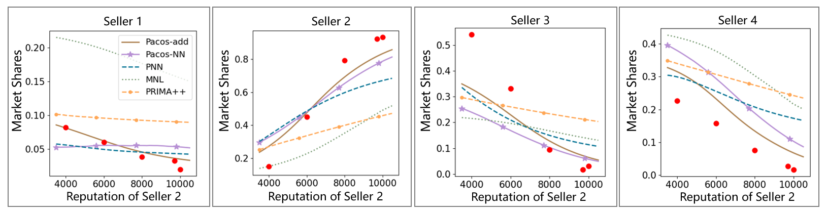
(a) adjusting the reputation of seller 2

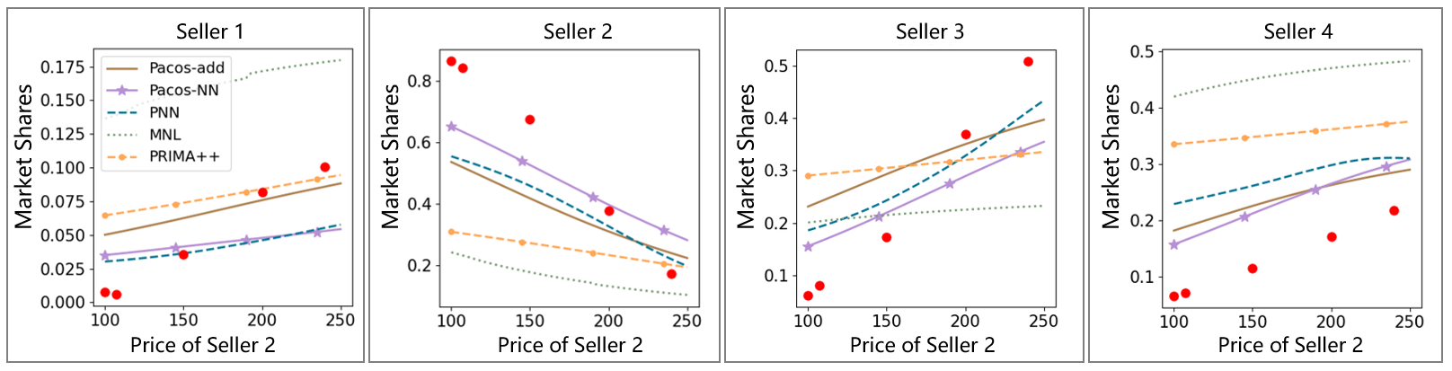
(b) adjusting the price of seller 2

Figure 2: The predicted trend in market share prediction task.

II-C The Update Rule

To analyze the impact of $K_{init}$ and $\Delta K$, in our experiment, we vary the value of $K_{init}$ and $\Delta K$ from 5 to 25, respectively, and the results of $sr(m=1)$ are shown in Fig. 1. It can be seen from Fig. 1 that the success rate is stable when $K_{init}$ and $\Delta K$ changes, indicating that the proposed model is not sensitive to the selection of $K_{init}$ and $\Delta K$.