Electronic states in quantum wires on the Möbius strip.

Abstract

In this work, we study the properties of an electron constrained on wires along the Möbius strip. We considered wires around the strip and along the transverse direction, across the width of the strip. For each direction, we investigate how the curvature modifies the electronic states and their corresponding energy spectrum. At the center of the strip, the wires around the surface form quantum rings whose spectrum depends on the strip radius $a$. For wires at the edge of the strip, the inner edge turns into the outer edge. Accordingly, the curvature yields localized states in the middle of the wire. Along the strip width, the effective potential exhibits a parity symmetry breaking leading to the localization of the bound state on one side of the strip.

I Introduction

In the latest decades, the investigation of the low-dimensional system had attracted much attention due to their unconventional properties [1, 2]. Geometry has crucial importance in two-dimensional systems, such as in flat graphene, carbon nanotubes, or even in one-dimensional quantum wires and quantum rings. Indeed, the curvature of the graphene surface modifies the electronic, elastic, and thermal properties of the material [1, 2, 3]. This new field, named curvatronics, explores new features and phenomena driven by the curvature of low-dimensional samples.

Among the two-dimensional geometries proposed, a graphene Möbius strip has been studied both theoretical and experimentally [4, 5, 6, 7, 8]. The graphene Möbius strip is a single-sided surface built by gluing the two ends of graphene ribbons, after rotating one end by $180^{o}$. If one starts in one edge of the Möbiusstrip and takes a $360^{o}$ rotation, it ends up on the other edge of the strip. Thus, besides the curvature, the asymmetry of the Möbius strip ought to influence the electronic properties.

The influence of curvature on the quantum dynamics of a particle constrained on surfaces is a long-standing issue [9, 10, 11]. One widely used approach is the so-called squeezing method, wherein the Schrödinger equation on the surface is obtained by considering a small width $\epsilon$ to the surface and taking the limit $\epsilon\rightarrow 0$. As a result, a curvature-dependent potential is obtained, the so-called da Costa potential [11, 12]. The effects of the da Costa potential have been studied on several surfaces, such as the catenoid[13], helicoid[12], and nanotorus[14], among others.

The electronic features of the whole Möbius strip have been previously explored in other works, for instance, in the Ref. [15]. In the ref. [16, 17] only the minimal coupling was considered. More recently, the Laplace-Beltrami operator on the curved Möbius strip was investigated at the limit when the strip width tends to zero, at the limit of thin strips[18].

In this work, we analyze the features of an electron constrained in a wire on the Möbius strip. In fact, we can use the curvature of the Möbius strip to build one-dimensional structures on this surface and analyze the electronic structures of an electron restricted to these quantum wires. The electron that is constrained to move in the longitudinal direction will move in a quantum wire around the Möbius strip while being influenced by the bending of the strip in that direction, whereas an electron constrained in the transverse direction will move in a quantum wire in the width of the strip, also felt the influence of curvature in that direction. Thus, we consider two possible wires: one along the length of the strip or along the width of the strip. For the former, we vary the angular variable $\theta$ while keeping the width variable $u$ constant. For the latest, we fix $\theta$ and vary $u$. For each wire, we obtain the effective potential containing the curvature influence of such wire, and we analyze the wave functions and their corresponding energy levels. In addition, the symmetries inherited or broken by the geometry upon the electronic states are discussed.

This paper is organized as follows: In section II, we present a brief review of the differential geometry of the Möbius strip. In section III, we obtain the effective Hamiltonian containing the da Costa potential and discuss their symmetries and the appropriate boundary conditions of our problem. In section IV, we define the wires around the strip, and along the width of the strip. For each wire, we studied the properties of the eigenfunctions and their respective spectrum. We also discuss some limiting cases in each wire, i.e., large width compared to the strip radius, etc. Finally, additional considerations and future perspectives are presented in section V.

II The Möbius Strip

In this section, we will provide a brief geometric description of the Möbius strip and construct a curvilinear coordinate system on its surface. In cylindrical coordinates, a Möbius Strip with inner radius $a$, and width $2w$, can be parameterized as,

$$\vec{\mathbf{r}}(u,\theta)=\left(a+uCos\frac{\theta}{2}\right)\hat{\rho}+uSen\frac{\theta}{2}\hat{k}$$ (1)

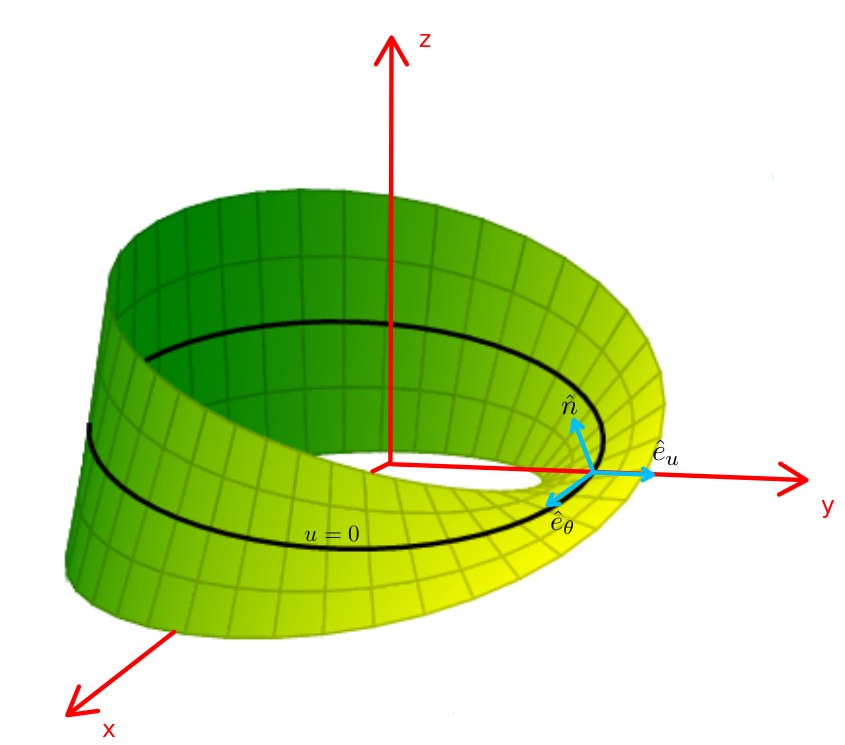
Figure 1: Möbius strip with a local reference frame determined by the tangent vectors $\hat{\mathbf{e}}_{u}$, $\hat{\mathbf{e}}_{\theta}$, and the normal vector $\hat{\mathbf{n}}$.

where $u$ is the coordinate that measures the distance between a point on the strip and its inner circle, measured along the strip, with $-w<u<w$, and $\theta$ runs around the strip, this is $0\leq\theta\leq 2\pi$.

The vectors which are tangents to the surface are described by,

$$\begin{cases}\hat{\mathbf{e}}_{u}=\frac{\partial\vec{\mathbf{r}}}{\partial u}=\cos\dfrac{\theta}{2}\hat{\rho}+\sin\frac{\theta}{2}\hat{k}\\ \hat{\mathbf{e}}_{\theta}=\frac{\partial\vec{\mathbf{r}}}{\partial\theta}=-\frac{u}{2}\sin\frac{\theta}{2}\hat{\rho}+(a+u\cos\frac{\theta}{2})\hat{\theta}+\frac{u}{2}\cos\frac{\theta}{2}\hat{k}.\end{cases}$$ (2)

And the normal vector is given by:

$$\hat{\mathbf{n}}=\dfrac{\hat{\mathbf{e}}_{u}\times\hat{\mathbf{e}}_{\theta}}{|\hat{\mathbf{e}}_{u}\times\hat{\mathbf{e}}_{\theta}|},$$ (3)

that is,

$$\hat{\mathbf{n}}=\dfrac{1}{\beta}[-\sin\dfrac{\theta}{2}(a+u\cos\dfrac{\theta}{2})\hat{\rho}-\dfrac{u}{2}\hat{\theta}+\cos\dfrac{\theta}{2}(a+u\cos\dfrac{\theta}{2})\hat{k}],$$ (4)

where,

$$\beta(u,\theta)=\sqrt{\frac{u^{2}}{4}+\Big{(}a+u\cos\frac{\theta}{2}\Big{)}^{2}}.$$ (5)

In this way, we can build a coordinate system on the Möbius strip determined by unit vectors and orthogonal to each other, $\hat{\mathbf{e}}_{u}$, $\hat{\mathbf{e}}_{\theta}$, and $\hat{\mathbf{n}}$.

From the tangent vectors, we define the metric tensor for our surface $g_{ij}=\hat{\mathbf{e}}_{i}\cdot\hat{\mathbf{e}}_{j}$. In the matrix notation, the metric tensor takes the form

$$g_{ij}=\begin{pmatrix}1&0\\ 0&\beta^{2}(u,\theta)\end{pmatrix},$$ (6)

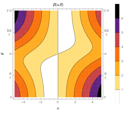
Figure 2: Metric function $\beta(u,\theta)$.

It is worthwhile to mention that the metric is not invariant under a parity transformation $(u,\theta)\rightarrow(-u,-\theta)$. However, $\beta$ is invariant under an inversion along the width and a rotation under a $2\pi$ angle, i.e., $\beta(-u,\theta+2\pi)=\beta(u,\theta)$. In addition, the metric is invariant under the transformation $(u,\theta)\rightarrow(-u,2\pi-\theta)$. These symmetries can be seen in fig.(2).

The curvature of surfaces is given by calculating the mean and Gaussian curvatures, which are obtained from calculating the first and second fundamental forms[19]. The elements of the second fundamental form are obtained by means of $h_{ij}=\partial_{i}\hat{\mathbf{e}}_{j}\cdot\hat{\mathbf{n}}$, from which we obtain the elements of the matrix from Weingartein[19]:

$$h^{i}_{j}=\dfrac{1}{\beta^{2}}\begin{pmatrix}0&\dfrac{a}{2\beta}\\ \dfrac{a}{2\beta}&\dfrac{\sin\dfrac{\theta}{2}(4\beta^{2}+u^{2})}{4\beta}\end{pmatrix},$$ (7)

where $h^{i}_{j}=g^{ik}h_{kj}$. The Gaussian curvature is defined as $K=det(h^{i}_{j})$, and the mean curvature is given by $H=\dfrac{1}{2}Tr(h^{i}_{j}))$. For the Möbius strip, the curvature has the expression

$$H(u,\theta)=\dfrac{\sin(\theta/2)(4\beta^{2}+u^{2})}{8\beta^{3}},$$ (8)

and,

$$K(u,\theta)=-\dfrac{a^{2}}{4\beta^{4}}.$$ (9)

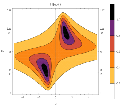
Figure 3: Mean curvature of a Möbius strip according to equation (10), where the result is varied for a Möbius strip of internal radius $a=1$, $-5\leq u\leq 5$, and $0\leq\theta\leq 2\pi$.

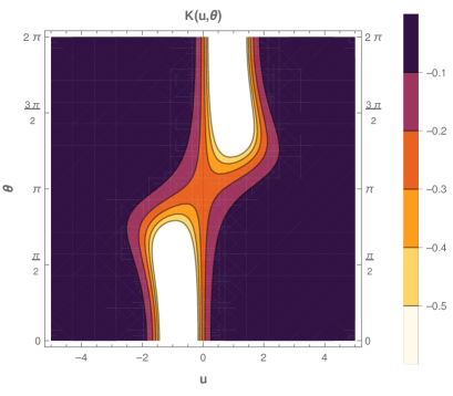
Figure 4: Gaussian curvature of a Möbius strip according to equation (11), where the result is varied for a Möbius strip of internal radius $a=1$, $-5\leq u\leq 5$, and $0\leq\theta\leq 2\pi$.

The behavior of the mean curvature $H$ and the Gaussian curvature $K$ with respect to $u$ and $\theta$ is showing in the fig.(3) and in the fig.(4), respectively. Note that the curvatures exhibit the symmetry under the transformation $(u,\theta)\rightarrow(-u,2\pi-\theta)$. Moreover, both curvatures are greater around the middle of the strip, near the angles $\theta=\pi/w$ and $\theta=\frac{3\pi}{2}$.

III Electron on Möbius Strip

In this section, we describe the dynamics of a constrained electron on the surface of a Möbius strip. A restricted electron in a surface, in the absence of external fields, is governed by the Hamiltonian [11, 13]

$$\mathcal{\hat{H}}=\frac{1}{2m^{*}}g^{ij}\hat{P}_{i}\hat{P}_{j}+V_{dC},$$ (10)

where $m^{*}$ is the effective mass of the electron, $\hat{P}_{i}:=-i\hbar\nabla_{i}$ is the momentum operator, and $V_{g}$ is a potential of geometric origin that corresponds to a contribution of the curvature in the Hamiltonian of the electron. The covariant derivative $\nabla_{i}$ of the momentum operator is given by $\nabla_{i}V^{j}:=\partial_{i}V^{j}+\Gamma^{j}_{ik}V^{k}$, where $\Gamma^{j}_{ik}=\dfrac{g^{jm}}{2}(\partial_{i}g_{mk}+\partial_{k}g_{mi}-\partial_{m}g_{ik})$ is the Christoffel symbol. Thus, the spinless stationary Schröndinger equations is

$$\frac{1}{2m^{*}}g^{ij}\{-\hbar^{2}[\partial_{i}\partial_{j}\psi-\Gamma^{k}_{ij}\partial_{k}\psi]\}+V_{g}\psi=E\psi.$$ (11)

The geometric potential $V_{g}$, known as da Costa potential, depends on the Gaussian curvature $K$ and the mean curvature $H$ by $V_{g}=V_{dC}=-\frac{\hbar^{2}}{2m^{*}}\left(H^{2}-K\right)$[11]. Thus, the da Costa potential in the Möbius strip is given by

$$V_{dC}=-\dfrac{\hbar^{2}}{2m^{*}}\Big{[}\dfrac{\sin^{2}(\theta/2)}{64\beta^{6}}(4\beta^{2}+u^{2})^{2}+\dfrac{a^{2}}{4\beta^{4}}\Big{]},$$ (12)

whose behavior is sketched in fig.(5).

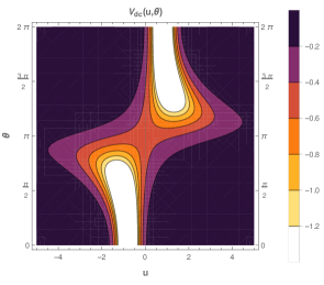
Figure 5: Geometric potential on the Möbius strip.

It is worthwhile to mention that the geometric potential exhibits the same symmetries and behavior of the mean and the gaussian curvatures.

Before proceeding in the study of the Schrödinger equation, let us analyze the symmetries of the Hamiltonian.

III.1 Symmetries

The Hamiltonian can be cast into the form

$$\mathcal{\hat{H}}=\dfrac{1}{2m}\Big{[}\hat{P}_{u}^{2}+\dfrac{1}{\beta^{2}}\hat{P}^{2}_{\theta}-i\hbar\dfrac{\partial_{u}\beta}{\beta}\hat{P}_{u}+i\hbar\dfrac{\partial_{\theta}\beta}{\beta^{3}}\hat{P}_{\theta}\Big{]}+V_{dC}.$$ (13)

It is worthwhile to mention that, unlike the catenoid, nanotubes, helicoid, and torus among others, the Möbius strip has no axial symmetry, i.e., the surface does not remain invariant under the transformation $\theta\rightarrow-\theta$. This asymmetry is inherited by the Hamiltonian (13), which now depends explicitly on $\theta$. The Hamiltonian dependence on $\theta$ means that the angular momentum with respect to the $z$ axis $L_{z}$ is no longer conserved. Accordingly, the $\hat{L}_{z}$ operator $\hat{L}_{z}=-\frac{i\hbar}{\beta^{2}}\frac{d}{d\theta}$ no longer commutes with the Hamiltonian (13). As a result, we cannot separate the wave function as $\Psi(u,\theta)=e^{im\theta}\psi(u)$.

Another noteworthy feature of the Hamiltonian (13) is that the presence of the first-derivative terms turns the Hamiltonian non-Hermitian. In fact,

$$\Big{[}\dfrac{i\hbar}{2m}\dfrac{\partial_{u}\beta}{\beta}\hat{P}_{u}\Big{]}^{\dagger}=\dfrac{-\hbar^{2}}{2m}\partial_{u}\left(\dfrac{\partial_{u}\beta}{\beta}\right)-\dfrac{i\hbar}{2m}\dfrac{\partial_{u}\beta}{\beta}\hat{P}_{u}$$ (14)

and similarly

$$\Big{[}\dfrac{i\hbar}{2m}\dfrac{\partial_{\theta}\beta}{\beta^{3}}\hat{P}_{\theta}\Big{]}^{\dagger}=\dfrac{-\hbar^{2}}{2m}\partial_{\theta}\left(\dfrac{\partial_{\theta}\beta}{\beta^{3}}\right)-\dfrac{i\hbar}{2m}\dfrac{\partial_{\theta}\beta}{\beta^{3}}\hat{P}_{\theta}$$ (15)

Since the Hamiltonian does not depend on the time, the Hamiltonian is invariant under the time-reversal symmetry $\mathcal{T}$, where $t\rightarrow-t$. This symmetry leads to the conservation of energy. Although the Hamiltonian is not invariant under parity transformation $(-u,-\theta)\rightarrow(u,\theta)$, the Hamiltonian inherits the combined symmetry $(-u,2\pi-\theta)\rightarrow(u,\theta)$. This symmetry can be considered as a modified Möbius parity transformation $\mathcal{P}_{M}$. Therefore, the Möbius strip is invariant under $\mathcal{P}_{M}\mathcal{T}$ transformation.

The non-hermiticity of the Hamiltonian (13) could lead to imaginary energy eigenvalues. However, as shown by some authors[20, 21], the $\mathcal{P}\mathcal{T}$ symmetry allows the existence of a real energy spectrum.

IV Quantum rings and quantum wires on a Möbius Strip

Figure 6: Effective potentials on the Möbius strip for fixed values of $u$ for a Möbius strip of length $L=5$ and inner radius $a=1$.

In the previous sections, we review the basic features of the Möbius strip geometry and explored the properties of the electron Hamiltonian. In this section, we define wires on the Möbius strip wherein the electron will be free to move. The effects of the curvature of these wires upon the electron states will be investigated. Let us start with a wire along the $\theta$ direction.

IV.1 Electron in a quantum ring on the Möbius strip.

By fixing the variable $u$, the stationary Schrödinger equation $\hat{H}\Psi=E\Psi$ with Hamiltonian given by eq.(13) yields to

$$-\dfrac{1}{\beta^{2}}\dfrac{d^{2}\psi}{d\theta^{2}}+\dfrac{\partial_{\theta}\beta}{\beta^{3}}\dfrac{d\psi}{d\theta}-(H^{2}-K)\psi=\epsilon\psi,$$ (16)

where $\epsilon=\frac{2mE}{\hbar^{2}}$. Although having only derivatives with respect to $\theta$, the eq.(16) depends on the choice of $u$ fixed.

By performing the change of variable

$$v(u_{0},\theta)=\int{\beta(u_{0},\theta)d\theta},$$ (17)

the Schrödinger equation becomes

$$-\dfrac{d^{2}\psi(v)}{dv^{2}}+U(u_{0},v)\psi(v)=\epsilon\psi(v).$$ (18)

where $U(v,u_{0})=-\left(H^{2}(u_{0},v)-K(u_{0},v)\right)$ is the effective potential. The variable $v$ is the arc length for a given $u$.

In fig.(6) we plotted the effective potential along the angular wire for the same values of $u$. It is worthwhile to mention that, the effective potential is just the da Costa potential. Hence, if we consider a minimal coupling, where no geometric potential squeezing potential is present, the effective potential for the angular wire vanishes. In addition, note that the potential is asymmetric as we change $u_{0}\rightarrow-u_{0}$. Thus, the choice of $u_{0}$ leads to the localization of the electron on one side or the other side of the strip.

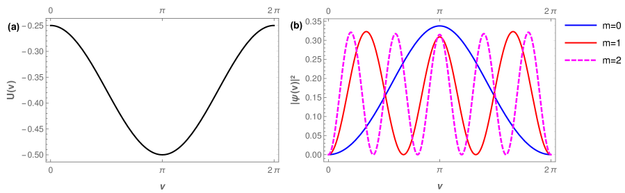
Figure 7: In graph (a) we have the effective potential for one for a particle at the center of the Möbius strip $(u=0)$, with inner radius $a=1$ and length $L=2\pi a$. In (b) we have the probability density for the first four eigenstates of the wave function of equation (46).

IV.1.1 Quantum ring at the center of the Möbius strip

Let us start our analysis with the most symmetric case, i.e., for u=0. This wire forms a quantum ring around the Möbius strip. Indeed, for $u=0$, the metric component $\beta(0,\theta)=a$.

For $u=0$, the effective Schrödinger equation eq.(18) becomes

$$-\ddot{\psi}(v)+\left[-\dfrac{1}{4a^{2}}\sin^{2}\left(\dfrac{v}{2a}\right)-\dfrac{1}{4a^{2}}\right]\psi(v)=\epsilon\psi(v).$$ (19)

Thus, the effective potential for a wire on the Möbius strip for $u=0$ is given by

$$U(v)=-\dfrac{1}{4a^{2}}-\dfrac{1}{4a^{2}}\sin^{2}\left(\dfrac{v}{2a}\right),$$ (20)

whose behavior is sketched in fig.(7). Note that the first term in eq.(20) represents the potential due to the curvature of the ring, whereas the second term steams from the Möbius strip curvature.

By redefining the variable $x=\dfrac{v}{2a}$ the Schrödinger equation along the ring at $u=0$ can be cast into a Mathieu equation

$$\dfrac{d^{2}\psi(x)}{dx^{2}}+[p-2q\cos(2x)]\psi(x)=0,$$ (21)

where,

$$\begin{cases}p=4a^{2}\epsilon+\dfrac{3}{2},\\ q=\dfrac{1}{4},\end{cases}$$ (22)

where $p$ and $q$ are parameters.

Mathieu’s equation has even index solutions denoted by $Ce_{2m}(a_{2m},q,x)$ and $Se_{2m}(b_{2m},q,x),$ $m=1,2,3...$, periodic in $\pi$, and odd index solutions denoted by $Ce_{2m+1}(a_{2m+1},q,x)$ and $Se_{2m+1}(b_{2m+1},q,x)$,$m=1,2,3...$, periodic in $2\pi$[22]. The complete solution to our problem is therefore:

$$\psi(x)=C_{1}Ce_{2m+1}(q,x)+C_{1}Se_{2m+1}(q,x).$$ (23)

Since the potential is periodic with a period of $2\pi$, we adopt the following boundary conditions

$$\psi(0)=\psi(2\pi)=0$$ (24)

By doing this the solution will depend only on the functions $Se_{2m+1}$. Finally, we arrive at the following normalized solution for the range $v\in[0,2\pi]$:

$$\psi(v)=\dfrac{1}{\sqrt{\pi}}Se_{2m+1}(\dfrac{v}{2a},\dfrac{1}{4})$$ (25)

The energy spectrum of the particle is related to the parameters $b_{2m+1}$ by

$$E_{2n+1}=\frac{\hbar^{2}}{2\mu a^{2}}\left(\frac{b_{2n+1}}{4}-\frac{3}{8}\right),$$ (26)

where $n=1,2,3..$ . Hence, the ground state has energy $E_{0}=-\frac{3\hbar^{2}}{16\mu a^{2}}$. Compared with the usual quantum circular ring, the wave function and energy spectrum of a particle of mass $\mu$ are:

$$\psi(\theta)=\frac{e^{im\theta}}{\sqrt{2\pi}},\quad E^{(ring)}_{m}=\frac{\hbar^{2}}{2\mu a^{2}}m^{2},\quad(m\in\mathbb{Z}),$$ (27)

where $m$ corresponds to the eigenvalue of the angular momentum of the particle in the $z$ direction. It is interesting to note that the spectrum of the particle in the center of the Möbius strip is not degenerate at any level, which does not occur with the particle in the circular ring, which from the ground state is doubly degenerate at each level. We plot the probability density functions of the first three eigenstates in figure (7).

IV.1.2 Quantum wire at the edges of the Möbius strip.

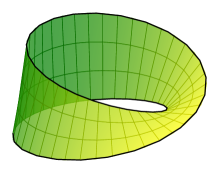
Figure 8: Quantum wire on the edge of the Möbius strip.

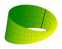
Figure 9: Quantum wire the width of the Möbius strip.

Let us now consider the motion of the electron in a wire at the edge of the strip. For a strip with a width w=2, $u$ goes from -1 to 1, and the maximum values of $u$, therefore, represent the edge of the strip. The wire is not a close loop (ring), due to the $4\pi$ symmetry of the Möbius strip. The Schrödinger equation (16), for $u=\pm 1$, is therefore

$$\begin{split}-\dfrac{1}{\beta^{2}_{u=\pm 1}}\dfrac{d^{2}\psi}{d\theta}-\dfrac{\pm(1\pm\cos\frac{\theta}{2})\sin\frac{\theta}{2}}{2\beta^{4}_{u=\pm 1}}\dfrac{d\psi}{d\theta}\\ -\left[\dfrac{1}{4\beta^{4}_{u=\pm 1}}-\dfrac{(1+4\beta_{u=\pm 1})^{2}\sin^{2}\frac{\theta}{2}}{64\beta^{6}_{u=\pm 1}}\right]\psi=\psi\epsilon,\end{split}$$ (28)

where $\beta^{2}_{u=\pm 1}=\sqrt{\frac{1}{4}+(1\pm\cos\frac{\theta}{2})^{2}}$.

The Schrödinger equation (28) also has a term dependent on the first order derivative in $\theta$. Then, performing the change of variable (17) we obtain a Schödinger equation in the variable $v$. Since the expression of the effective potential in $v$ is rather cumbersome, we present only the graphics for the potentials and their respective wave functions.

In fig.(10), the effective potential is plotted for $a=1$ and $L=5$. The potential exhibits a symmetric well around the origin $v=0$. The ground state has a bell shape localized at the origin. On the other hand, the first excited state in two points is displaced symmetrically from the origin, as shown in fig.(11).

The potential changes drastically as we reduce the inner radius $a$. In the figure (13), we plotted the effective potential for $a=0.5$, where a barrier arises near the origin. As a result, the wave function for the ground state becomes shifted from the $v=0$.

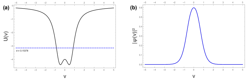
Figure 10: (a) Effective potential at the edge of a Möbius strip (solid black line), and energy value of the first restricted state (dashed blue line). (b) The probability density function for the first bound state on the edge of the Möbius strip(solid blue line). Results for a Möbius strip with inner radius $a=1$ and length $L=5$.

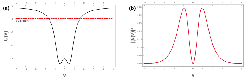
Figure 11: (a) Effective potential at the edge of a Möbius strip (solid black line), and energy value of the second restricted state (dashed red line). (b) The probability density function for the second bound state on the edge of the Möbius strip (solid red line). Results for a Möbius strip with inner radius $a=1$ and length $L=5$.

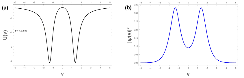
Figure 12: (a) Effective potential at the edge of a Möbius strip (solid black line), and energy value of the first restricted state (dashed blue line). (b) The probability density function for the first bound state on the edge of the Möbius strip (solid blue line). Results for a Möbius strip with inner radius $a=0.5$ and length $L=5$.

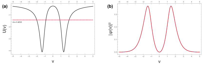
Figure 13: (a) Effective potential at the edge of a Möbius strip (solid black line), and energy value of the second restricted state (dashed red line). (b) The probability density function for the second bound state on the edge of the Möbius strip (solid red line). Results for a Möbius strip with inner radius $a=0.5$ and length $L=5$.

IV.1.3 Quantum wire along the Möbius strip width

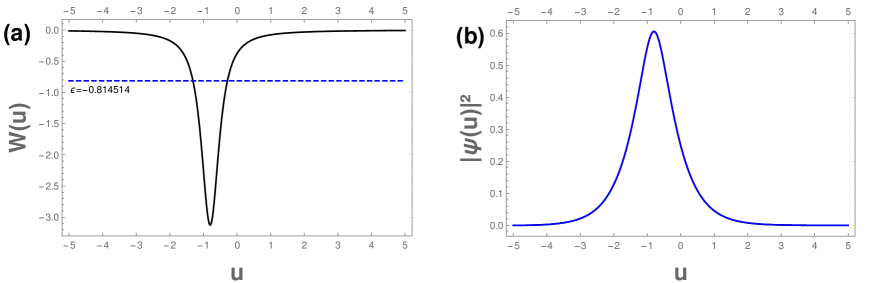
Figure 14: (a) Effective potential at the width of Möbius strip for $\theta_{0}=0$ (solid black line ) and energy value of the bound state (dashed blue line). (b) Probability density of the bound state at the width of Möbius strip. We use $a=1$ and $w=10$.

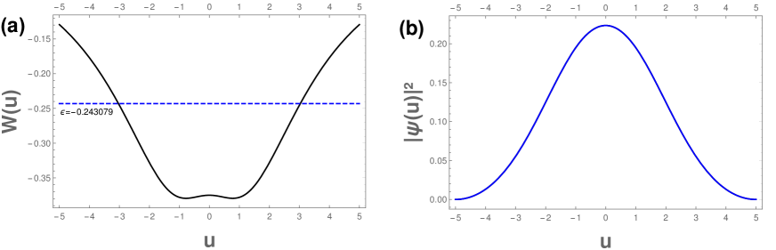
Figure 15: (a) Effective potential at the width of Möbius strip for $\theta_{0}=\pi$ (solid black line ) and energy value of the bound state (dashed blue line). (b) Probability density of the bound state at the width of Möbius strip. We use $a=1$ and $w=10$.

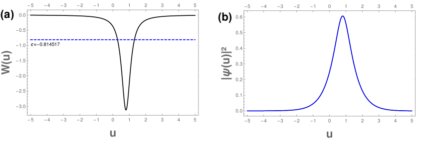
Figure 16: (a) Effective potential at the width of Möbius strip for $\theta_{0}=2\pi$ (solid black line ) and energy value of the bound state (dashed blue line). (b) Probability density of the bound state at the width of Möbius strip. We use $a=1$ and $w=10$.

Now let us consider the electron constrained to move along wires in the $u$ direction. We investigate how the wave function will be modified by the Möbius strip curvature.

By fixing the coordinate $\theta$, the Schrödinger equation reads

$$-\dfrac{d^{2}\psi}{du^{2}}-\dfrac{\partial_{u}\beta}{\beta}\dfrac{d\psi}{du}-(H^{2}-K)\psi=\epsilon\psi.$$ (29)

This equation can be further simplified by considering the following change on the wave function

$$\psi(u)=\psi(u,\theta_{0})=\frac{1}{\sqrt{\beta(u,\theta_{0})}}\phi(u).$$ (30)

The resulting Schrödinger equation for the function $\phi(u)$ has the form

$$-\frac{d^{2}\phi(u)}{du^{2}}+W(u,\theta_{0})\phi(u)=\epsilon\phi(u),$$ (31)

where the effective potential is given by

$$\begin{split}W(u,\theta_{0})=\left(\dfrac{\partial_{u}\beta}{2\beta}\right)_{|\theta=\theta_{0}}^{2}+\partial_{u}\left(\dfrac{\partial_{u}\beta}{2\beta}\right)_{|\theta=\theta_{0}}\\ -\left(H^{2}(u,\theta_{0})-K(u,\theta_{0})\right).\end{split}$$ (32)

We plot the effective potential along the $u$ direction $w(u)$ in eq.(32) for some fixed values of $\theta$. In the fig.(14), the wire is located at $\theta=0$. The potential exhibits a single well shifted to the left, towards the inner portion of the strip. The respective wave function is then, localized around this inner point. For $\theta=\pi$, shown in fig.(15), the potential well is symmetric with respect to the origin $u=0$. The wider potential allows the wave function to spread along the wire. For $\theta=2\phi$, both the potential well and the wave function are shifted to the right of the origin, as seen in fig.(16).

The behavior described above shows that the directional dependence of the Möbius strip geometry enables us to devise quantum wires wherein the density of states is controlled by the position and the curvature of the strip.

V Final remarks and perspectives

In this work, we studied the effects of the curvature of quantum wires constrained on the Möbius strip upon the electron properties. The advantage of considering the wire on the surface stems from the fact that the geometric potential depends not only on the wire curvature but on the surface curvature as well. Moreover, the electronic properties are modified by the twist and the symmetries of the Möbius strip.

By considering a wire along the length of the strip at the center, i.e., for $u=0$, the wire forms a ring whose effective potential has a ground state localized symmetrically around $\theta=\pi$. On the other hand, the excited states are more affected by the ring curvature $1/a$. For a wire on the edge of the strip, the states are localized around $\theta=0$. If the inner radius $a$ is reduced compared to the strip width $w$, the ground state gets localized in two symmetrical points around the origin.

We also considered wires along the strip width, i.e., for $\theta$ fixed. The anisotropy of the Möbius strip turns the effective potential highly dependent on the chosen angle. For $\theta=0$, the ground state is localized on the inner side of the strip, i.e., $u<0$. As the angle $\theta$ varies from $0$ to $2\pi$, the wave function is shifted from the inner to the outer side, i.e., for $u>0$.

The present work suggests further investigations. For instance, the effects of the curvature of the strip with multiple twists or the inclusion of external magnetic or electric fields could provide a way to tuning and control the density of states at other points along the strip. Moreover, the effects of the spin, by means of the Dirac or the Pauli equation seem promising.

Data Availability

The datasets generated during and/or analysed during the current study are available from the corresponding author on reasonable request

References

- Geim and Novoselov [2007] A. K. Geim and K. S. Novoselov, The rise of graphene, Nature materials 6, 183 (2007).
- Katsnelson [2012] M. I. Katsnelson, Graphene: Carbon in Two Dimensions (Cambridge University Press, 2012).
- Neto et al. [2009] A. C. Neto, F. Guinea, N. M. Peres, K. S. Novoselov, and A. K. Geim, The electronic properties of graphene, Reviews of modern physics 81, 109 (2009).
- Guo et al. [2009] Z. Guo, Z. Gong, H. Dong, and C. Sun, Möbius graphene strip as a topological insulator, Physical Review B 80, 195310 (2009).
- Wang et al. [2010] X. Wang, X. Zheng, M. Ni, L. Zou, and Z. Zeng, Theoretical investigation of möbius strips formed from graphene, Applied Physics Letters 97, 123103 (2010).
- Caetano et al. [2008] E. W. Caetano, V. N. Freire, S. Dos Santos, D. S. Galvao, and F. Sato, Möbius and twisted graphene nanoribbons: Stability, geometry, and electronic properties, The Journal of chemical physics 128, 164719 (2008).
- Zhang et al. [2017] X. Zhang, B. Tian, W. Zhen, Z. Li, Y. Wu, and G. Lu, Construction of möbius-strip-like graphene for highly efficient charge transfer and high active hydrogen evolution, Journal of catalysis 354, 258 (2017).
- Yang et al. [2018] K. Yang, C. Zhang, X. Zheng, X. Wang, and Z. Zeng, The stability of graphene-based möbius strip with vacancy and at high-temperature, International Journal of Modern Physics B 32, 1850350 (2018).
- DeWitt [1957] B. S. DeWitt, Dynamical theory in curved spaces. i. a review of the classical and quantum action principles, Reviews of modern physics 29, 377 (1957).
- Jensen and Koppe [1971] H. Jensen and H. Koppe, Quantum mechanics with constraints, Annals of Physics 63, 586 (1971).
- da Costa [1981] R. da Costa, Quantum mechanics of a constrained particle, Physical Review A 23, 1982 (1981).
- de Lima et al. [2021] J. de Lima, E. Gomes, F. da Silva Filho, F. Moraes, and R. Teixeira, Geometric effects on the electronic structure of curved nanotubes and curved graphene: the case of the helix, catenary, helicoid, and catenoid, The European Physical Journal Plus 136, 1 (2021).
- Silva et al. [2020a] J. E. G. Silva, J. Furtado, T. Santiago, A. C. Ramos, and D. da Costa, Electronic properties of bilayer graphene catenoid bridge, Physics Letters A 384, 126458 (2020a).
- Silva et al. [2020b] J. E. G. Silva, J. Furtado, and A. C. A. Ramos, Electronic properties of a graphene nanotorus under the action of external fields, The European Physical Journal B 93, 1 (2020b).
- Gravesen and Willatzen [2005] J. Gravesen and M. Willatzen, Eigenstates of möbius nanostructures including curvature effects, Physical Review A 72, 032108 (2005).
- Miliordos [2011] E. Miliordos, Particle in a möbius wire and half-integer orbital angular momentum, Physical Review A 83, 062107 (2011).
- Li and Ram-Mohan [2012] Z. Li and L. R. Ram-Mohan, Quantum mechanics on a möbius ring: Energy levels, symmetry, optical transitions, and level splitting in a magnetic field, Physical Review B 85, 10.1103/physrevb.85.195438 (2012).
- Kalvoda et al. [2020] T. Kalvoda, D. Krejčiřík, and K. Zahradova, Effective quantum dynamics on the möbius strip, Journal of Physics A: Mathematical and Theoretical 53, 375201 (2020).
- Spivak [1999] M. Spivak, A comprehensive introduction to differential geometry, vol. ii, 3rd edn. publish or perish, Inc., Houston (1999).
- Bender [2007] C. M. Bender, Making sense of non-hermitian hamiltonians, Reports on Progress in Physics 70, 947 (2007).
- Bender and Boettcher [1998] C. M. Bender and S. Boettcher, Real spectra in non-hermitian hamiltonians having p t symmetry, Physical review letters 80, 5243 (1998).
- Morse and Feshbach [1954] P. M. Morse and H. Feshbach, Methods of theoretical physics, American Journal of Physics 22, 410 (1954).