Exploration of the search space of Gaussian graphical models for paired data

Abstract

We consider the problem of learning a Gaussian graphical model in the case where the observations come from two dependent groups sharing the same variables. We focus on a family of coloured Gaussian graphical models specifically suited for the paired data problem. Commonly, graphical models are ordered by the submodel relationship so that the search space is a lattice, called the model inclusion lattice. We introduce a novel order between models, named the twin order. We show that, embedded with this order, the model space is a lattice that, unlike the model inclusion lattice, is distributive. Furthermore, we provide the relevant rules for the computation of the neighbours of a model. The latter are more efficient than the same operations in the model inclusion lattice, and are then exploited to achieve a more efficient exploration of the search space. These results can be applied to improve the efficiency of both greedy and Bayesian model search procedures. Here we implement a stepwise backward elimination procedure and evaluate its performance by means of simulations. Finally, the procedure is applied to learn a brain network from fMRI data where the two groups correspond to the left and right hemispheres, respectively.

Keywords: Brain network; coloured graphical model; lattice; partial order; principle of coherence; RCON model.

1 Introduction

A Gaussian graphical model (GGM) is a family of multivariate normal distributions whose conditional independence structure is represented by an undirected graph. The vertices of the graph correspond to the variables and every edge missing from the graph implies that the corresponding entry of the concentration matrix, that is the inverse of the covariance matrix, is equal to zero; see Lauritzen (1996). Gaussian graphical models are widely applied to the joint learning of multiple networks, where the observations come from two or more groups sharing the same variables. The association structure of each group is represented by a network and it is expected that there are similarities between the groups. In this framework, the literature has mostly focused on the case where the groups are independent so that every network is a distinct unit, disconnected from the other networks; see Tsai et al. (2022) for a recent review. The problem of multiple dependent groups was considered by Xie et al. (2016), where the cross-graph dependence between groups is modelled by means of a latent vector representing systemic variation manifesting simultaneously in all groups; see also Zhang et al. (2022). We focus on the specific case of paired data, with exactly two dependent groups. Paired data commonly arise in paired design studies, where each subject is measured twice at two different time points or under two different conditions. A relevant example comes from cancer genomics where control samples are often obtained from histologically normal tissues adjacent to the tumor (NAT) (Aran et al., 2017). Paired data settings also arise from matched observational studies as well as in the analysis of brain networks where groups correspond to the two brain hemispheres (Ranciati et al., 2021).

Ranciati et al. (2021) and Roverato and Nguyen (2022) approached the problem of the joint learning of graphical models for paired data by considering a single coloured GGM comprising the variables of both the first and the second group. In this way, the resulting model has a graph for each of the two groups and the cross-graph dependence is explicitly represented by the edges across groups.

Coloured GGMs (Højsgaard and Lauritzen, 2008) are undirected graphical models with additional symmetry restrictions in the form of equality constraints on the parameters, which are then depicted on the dependence graph of the model by colouring of edges and vertices. Equality constraints allow one to disclose symmetries concerning both the structure of the network and the values of parameters associated with vertices and edges and, in addition, have the practical advantage of reducing the number of parameters. To this aim, Roverato and Nguyen (2022) introduced a subfamily of coloured GGMs specifically designed to suit the paired data problem that they called RCON models for paired data (PD-RCON).

Although the symmetry restrictions implied by a coloured GGM may usefully reduce the model dimension, the problem of model identification is much more challenging than with classical GGMs because both the dimensionality and the complexity of the search spaces highly increase; see Gao and Massam (2015), Massam et al. (2018), Li et al. (2020) and references therein. For the construction of efficient model selection methods it is therefore imperative to understand the structure of model classes.

A statistical model is a family of probability distributions, and if a model is contained in another model then it is called a submodel of the latter. We can also say that a model is “larger” than any of its submodels, and model inclusion is typically used to embed a model class with a partial order. In this way, one can easily obtain that the family of GGMs forms a complete distributive lattice. Gehrmann (2011) considered four relevant subfamilies of coloured GGMs and showed that they constitute a lattice with respect to model inclusion. However, the structure of such lattices are rather complicated and this makes the identification of neighbouring models, and therefore the implementation of procedures for the exploration of model spaces, much less efficient than for classical GGMs. Furthermore, none of the existing lattices of coloured GGMs satisfies the distributivity property, which is a fundamental property that facilitates the implementation of efficient procedures and representation in lattices; see, among others, Habib et al. (2001) and Davey and Priestley (2002). Roverato and Nguyen (2022) showed that, under the model inclusion order, the class of PD-RCON models identifies a proper complete sublattice of the lattice of coloured graphical models, although also in this case the distributive property is not satisfied.

We introduce a novel partial order for the class of PD-RCON models that coincides with the model inclusion order if two models are model inclusion comparable but that also includes order relationships between certain models which are model inclusion incomparable. We show that the class of PD-RCON models forms a complete lattice also with respect to this order, that we call the twin lattice. The twin lattice is distributive and its exploration is more efficient than that of the model inclusion lattice. Hence, the twin lattice can be used to improve the efficiency of procedures, either Bayesian and frequentist, which explore the model space moving between neighbouring models. More specifically, the focus of this paper is on stepwise greedy search procedures, and we show how the twin lattice can be exploited to improve efficiency in the identification of neighbouring submodels.

One way to increase the efficiency of greedy search procedures is by applying the, so-called, principle of coherence (Gabriel, 1969) that is used as a strategy for pruning the search space. We show that for the family of PD-RCON models the twin lattice allows a more straightforward implementation of the principle of coherence and, in fact, the twin lattice seems to represent the natural structure for the exploration of PD-RCON model spaces.

We implement a stepwise backward elimination procedure with local moves on the twin lattice which satisfies the coherence principle, and we show that it is more efficient than an equivalent procedure on the model inclusion lattice. This procedure is implemented in the statistical programming language R and its behavior is investigated on simulated data. Finally, this procedure is applied to the identification of the brain network from fMRI data.

The rest of the paper is organized as follows. Background on lattice theory, coloured graphical models and the structure of their model space is given in Section 2, whereas Section 3 introduces the family of RCON models for paired data. In Section 4, we introduce the twin lattice, derive its properties and describe its relationships with the model inclusion lattice. Section 5 deals with the dimension of the search space and the implementation of the principle of coherence. The greedy search procedure is described in Section 6 and then, in Section 7, this is applied both on simulated data and on fMRI data to learn a brain network. Finally, Section 8 contains a brief discussion. Proofs are deferred to Section S-6 of the Supplementary Material.

2 Background and Notation

2.1 Partial orders and lattices

In this section, we review the elements and notation of lattice theory as required for this paper, and refer to Davey and Priestley (2002) for a more comprehensive account.

A partially ordered set, or poset, $\langle A,\preceq\rangle$ is a structure where $A$ is a set and $\preceq$ is a partial order on $A$. If the elements $a,b\in A$ are such that $a\preceq b$ with $a\neq b$, then we write $a\prec b$ and say that $a$ is smaller than $b$. Furthermore, if it also holds that there is no element $c\in A$ such that $a\prec c\prec b$ then we say that $a$ is covered by $b$ and write $a\mathrel{\ooalign{$\prec$\cr\raise 0.08612pt\hbox{$\cdot\mkern 0.1mu$}\cr}}b$. If both $a\not\preceq b$ and $b\not\preceq a$ then $a$ and $b$ are incomparable.

An element $a\in A$ is called an upper bound of the subset $H\subseteq A$ if it has the property that $h\preceq a$ for all $h\in H$ and, furthermore, it is the supremum of $H$, denoted by $a=\sup H$, if every upper bound $b$ of $H$ satisfies $a\preceq b$. Accordingly, $a\in A$ is a lower bound of $H$ if $a\preceq h$ for all $h\in H$, and it is the infimum of $H$, $a=\inf H$, if for every lower bound $b$ of $H$ it holds that $b\preceq a$. If for a poset $\langle A,\preceq\rangle$ the element $\sup A$ exists, then it is called the maximum element, or the unit, of $A$ and denoted by $\hat{1}$. Dually, if $\inf A$ exists, then this element is called the minimum element, or the zero, of $A$ and denoted by $\hat{0}$.

A poset $\langle A,\preceq\rangle$ is called a lattice if $\inf H$ and $\sup H$ exist for every finite nonempty subset $H$ of $A$. A lattice is called complete if also both $\inf A$ and $\sup A$ exist. If $\langle A,\preceq\rangle$ is a lattice, then for every pair of elements $a,b\in A$, we write $a\wedge b$ for $\inf\{a,b\}$ and $a\vee b$ for $\sup\{a,b\}$ and refer to $\wedge$ as the meet operation and to $\vee$ as the join operation. A lattice $A$ is called distributive if the operations of join and meet distribute over each other; formally, if for all $a,b,c\in A$, $a\vee(b\wedge c)=(a\vee b)\wedge(a\vee c)$. Finally, it is useful to represent the structure of a lattice graphically by means of an Hasse diagram that is a graph with $A$ as vertex set and where two elements $a,b\in A$ are joined by an undirected edge, with the vertex $b$ appearing above $a$, whenever $a\mathrel{\ooalign{$\prec$\cr\raise 0.08612pt\hbox{$\cdot\mkern 0.1mu$}\cr}}b$; see Figures S-5 and S-6 of the Supplementary Material for examples.

2.2 Graphical models and coloured graphical models

For a finite set $V=\{1,\ldots,p\}$ we let $Y=Y_{V}$ be a continuous random vector indexed by $V$ and we denote by $\Sigma=(\sigma_{ij})_{i,j\in V}$ and $\Sigma^{-1}=\Theta=(\theta_{ij})_{i,j\in V}$ the covariance and concentration matrix of $Y$, respectively. An undirected graph with vertex set $V$ is a pair $G=(V,E)$ where $E$ is an edge set that is a set of unordered pairs of distinct vertices; formally $E\subseteq F_{V}$ with $F_{V}=\{(i,j)\mid i,j\in V\mbox{ and }i<j\}$. Thus, $F_{V}$ is the edge set of the complete graph, that is the graph in which each pair of distinct vertices is connected by an edge. Note that, when it is not clear from the context which graph is under consideration, we will write $V_{G}$ and $E_{G}$ to denote the vertex set and edge set of the graph $G$.

We say that the concentration matrix $\Theta$ is adapted to the graph $G$ if every missing edge of $G$ corresponds to a zero entry in $\Theta$; formally, $(i,j)\notin E$, with $i<j$, implies that $\theta_{ij}=\theta_{ji}=0$. A Gaussian graphical model (GGM) with graph $G$ is the family of Gaussian distributions whose concentration matrix is adapted to $G$; see Lauritzen (1996). We denote by $M\equiv M(V)$ the family of GGMs for $Y_{V}$ and by $M(G)\in M$ the GGM represented by the graph $G=(V,E)$.

A colouring of $G=(V,E)$ is a pair $(\mathcal{V},\mathcal{E})$ where $\mathcal{V}=\{V_{1},\ldots,V_{v}\}$ is a partition of $V$ into vertex colour classes and, similarly, $\mathcal{E}=\{E_{1},\ldots,E_{e}\}$ is a partition of $E$ into edge colour classes. Accordingly, $\mathcal{G}=(\mathcal{V},\mathcal{E})$ is a coloured graph. Similarly to the notation used for uncoloured graphs, we may write $\mathcal{V}_{\mathcal{G}}$ and $\mathcal{E}_{\mathcal{G}}$ to denote the vertex and edge colour classes of $\mathcal{G}$, respectively. In the graphical representation, all the vertices belonging to a same colour class are depicted of the same colour, and similarly for edges. Furthermore, in order to make coloured graphs readable also in black and white printing, we put a common symbol next to every vertex or edge of the same colour. The only exception to this rule is for vertices and edges belonging to colour classes with a single element, called atomic, which are all depicted in black with no symbol next to them.

Højsgaard and Lauritzen (2008) introduced coloured GGMs, which are GGMs with additional restrictions on the parameter space. The models are represented by coloured graphs, where parameters that are associated with edges or vertices of the same colour are restricted to being identical. In this paper we focus on the family of coloured GGMs known as RCON models (Højsgaard and Lauritzen, 2008) which place equality restrictions on the entries of the concentration matrix. More specifically, in the RCON model with coloured graph $\mathcal{G}=(\mathcal{V},\mathcal{E})$ every vertex colour class $V_{i}$, $i=1,\ldots,v$, identifies a set of diagonal concentrations whose value is constrained to be equal, and similarly for edge colour classes which identify subsets of off-diagonal concentrations. We denote by $\mathcal{M}\equiv\mathcal{M}(V)$ the family of RCON models for $Y_{V}$ and by $\mathcal{M}(\mathcal{G})\in\mathcal{M}$ the RCON model represented by $\mathcal{G}$.

We close this section by noticing that for the families of graphical models we consider here every model is uniquely represented by a coloured graph, and in the rest of this paper, with a slight abuse of notation, we will not make an explicit distinction between sets of model and sets of graphs, thereby equivalently writing, for example, $\mathcal{M}(\mathcal{G})\in\mathcal{M}$ and $\mathcal{G}\in\mathcal{M}$.

2.3 Exploration of the model space

The implementation of most model selection procedures requires the exploration of the space of candidate structures, i.e. of the model space. It is therefore fundamental to understand the structure of model spaces so as to improve efficiency and to identify suitable neighbouring relationships to be used in greedy search procedures. In the families of graphical models we consider, this is typically achieved by embedding the model space with the partial order defined through the model inclusion, i.e. the submodel, relationship thereby obtaining a lattice structure. In the rest of this section, we review the relevant properties of the model inclusion lattices of both undirected and coloured graphical models, and discuss their use in the exploration of model spaces.

Two well-known lattices which become relevant in this context are the so-called subset and partition lattices. The power set $\mathcal{P}ow(A)$ of any finite set $A$ is naturally embedded with the set inclusion order, $\subseteq$, and forms a complete distributive lattice. This is a well-known lattice structure whose meet and join operations can be efficiently computed because they are the set intersection $\cap$ and the set union $\cup$ operations, respectively (see Davey and Priestley, 2002). A partition of $A$ is a collection of nonempty, pairwise disjoint, subsets of $A$ whose union is $A$. The family of partitions $\mathcal{P}art(A)$ of a set $A$ is typically embedded with the partial order where the partition $P_{1}$ is smaller than $P_{2}$ if $P_{1}$ is finer than $P_{2}$, that is if every set in $P_{2}$ can be expressed as a union of sets in $P_{1}$. In this way, one obtains the so-called partition lattice, and it is well-understood that distributivity does not hold for this lattice and, furthermore, the implementation of the meet and of the join operations is more involved, and considerably less efficient, than in the subset lattice; see Canfield (2001) and Pittel (2000).

Given two graphs $G$ and $H$, with vertex set $V$, we write $M(H)\preceq_{s}M(G)$ to denote that $M(H)$ is a submodel of $M(G)$. For the family of GGMs, model inclusion coincides with the subset relationship between edge sets, so that for every pair of graphs, $G$ and $H$, with vertex set $V$, it holds that $M(H)\preceq_{s}M(G)$ if and only if $E_{H}\subseteq E_{G}$. Hence, $\langle M,\preceq_{s}\rangle$ coincides with the subset lattice of $F_{V}$ and, consequently, the meet and the join operations take an especially simple form because $M(G)\vee M(H)$ and $M(G)\wedge M(H)$ are the models represented by the graphs with edge sets $E_{G}\cup E_{H}$ and $E_{G}\cap E_{H}$, respectively. Furthermore, the lattice $\langle M,\preceq_{s}\rangle$ is complete and distributive.

Consider now the family $\mathcal{M}$ of RCON models for $Y_{V}$ and let $\mathcal{G}$ and $\mathcal{H}$ be two coloured graphs with vertex set $V$. It was shown by Gehrmann (2011) that $\mathcal{M}(\mathcal{H})$ is a submodel of $\mathcal{M}(\mathcal{G})$, i.e. $\mathcal{M}(\mathcal{H})\preceq_{s}\mathcal{M}(\mathcal{G})$, if and only if all of the three following conditions hold true,

1. the edge set of $\mathcal{H}$ is a subset of the edge set of $\mathcal{G}$;

2. every colour class in $\mathcal{V}_{\mathcal{H}}$ is a union of colour classes in $\mathcal{V}_{\mathcal{G}}$;

3. every colour class in $\mathcal{E}_{\mathcal{H}}$ is a union of colour classes in $\mathcal{E}_{\mathcal{G}}$;

and we remark that condition (S1) can be considered as redundant because, in fact, it is implied by (S3). Furthermore, Gehrmann (2011) showed that $\langle\mathcal{M},\preceq_{s}\rangle$ is a complete lattice, although non-distributive. Colour classes are partitions of the vertex and edge set, respectively, and Gehrmann (2011, eqn. 9) provided explicit rules for the computation of the meet $\mathcal{M}(\mathcal{G})\wedge\mathcal{M}(\mathcal{H})$ and the join $\mathcal{M}(\mathcal{G})\vee\mathcal{M}(\mathcal{H})$, which follow from the same operations in the partition lattice and share an equivalent level of computational complexity. The exploration of the space of RCON models is thus much more challenging than the exploration of GGMs because, firstly, as shown by Gehrmann (2011) the dimension of $\langle\mathcal{M},\preceq_{s}\rangle$ is much larger than that of $\langle M,\preceq_{s}\rangle$ and it grows super-exponentially with the number of variables and, secondly, the exploration of the space through neighbouring models, which requires the application of the meet and the join of models, is more computationally demanding than in $\langle\mathcal{M},\preceq_{s}\rangle$. Indeed, the existing procedures for learning coloured graphical models can deal with a small number of variables (Gehrmann, 2011) or impose substantial approximations (Li et al., 2018).

One way to avoid the explicit exploration of the model space is by using penalized likelihood methods as in Li et al. (2021) and Ranciati et al. (2021), which can be applied to problems of larger dimension. These procedures are not invariant to scalar multiplications of the variables and for this reason it is common practice to standardise the data to have unit sample variances; see, among others, Hastie et al. (2015, p. 8) and Carter et al. (2021). However, this preliminary step is problematic in paired data problems because RCON models are not invariant with respect to normalization of the variables and thus standardization will typically change the original structure of colour classes.

3 RCON models for paired data

Roverato and Nguyen (2022) introduced PD-RCON models, which is a subfamily of RCON models specifically designed to deal with paired data. In this section, we introduce the twin-pairing function that allows us to deal efficiently with the paired data setting, and use it to define the family of PD-RCON models. We start with a small instance of paired data problem that will be used hereafter as a running example.

Example 1 (Frets’ Heads).

Whittaker (1990, Section 8.4) fitted a GGM to the Frets’ Heads data which consist of measurements of the head Height and head Breadth of the first and second adult sons in a sample of 25 families. Variables are therefore naturally split into the variables associated with the first son, $Y_{H}$ and $Y_{B}$, and the second son, $Y_{H^{\prime}}$ and $Y_{B^{\prime}}$, thereby identifying the $L$eft and $R$ight groups depicted in Figure 1(a). Note that, for the presentation of the results below it is convenient to use a numerical vertex set, that is $V=\{1,2,3,4\}$; however, in order to improve readability, in this example we also add subscripts and write $L=\{1_{H},2_{B}\}$ and $R=\{3_{H^{\prime}},4_{B^{\prime}}\}$.

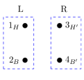
(a)

(b)

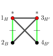
(c)

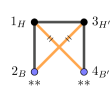
(d)

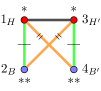
(e)

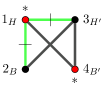
(f)

Figure 1: Frets’ Heads example: (a) gives the partition of the vertex set into the two groups; the graphs (b) to (e) are PD-CGs whereas (f) is a coloured graph but not a PD-CG.

In paired data problems, every variable in $Y_{V}$ has an homologous, or twin, variable in $Y_{V}$, and the twin-pairing function $\tau$, or twin function for short, associates every element $i\in V$ with its twin $\tau(i)\in V$, in such a way that if $\tau(i)=j$ then $\tau(j)=i$. We then naturally extend the use of the twin function to edges as well as to collections of vertices and edges. Formally, for $(i,j)\in F_{V}$ we let $\tau(i,j)=(\tau(i),\tau(j))$ whereas for $A\subseteq V$ we set $\tau(A)=\{\tau(i)\mid i\in A\}$ and if $E\subseteq F_{V}$ then $\tau(E)=\{\tau(i,j)\mid(i,j)\in E\}$, with the convention that $\tau(\emptyset)=\emptyset$. Note that it may happen that $\tau(i,j)=(\tau(i),\tau(j))$ is such that $\tau(i)>\tau(j)$ and in this case we will implicitly assume that the endpoints of such pairs are reversed, so as to obtain a proper edge belonging to $F_{V}$.

The twin function can be used to partition the set $V$ into two sets, $L\cup R=V$, with $L\cap R=\emptyset$, such that $\tau(L)=R$. This partition is not unique, and the theory developed in this paper requires the identification of one of such partitions, which can be arbitrarily chosen. Nevertheless, there typically exists a natural partition where $L$ is associated with the first group and $R$ with the second group and in our examples we will, without loss of generality, always refer to such natural partition. Accordingly, to facilitate the interpretation of a model, we will depict the coloured graph with vertices $L$ on the $L$eft and vertices $R$ on the $R$ight.

In paired data problems the focus is in similarities and differences between the two groups. Any vertex $i\in V$ and its twin $\tau(i)$ are associated with the diagonal entries $\theta_{ii}$ and $\theta_{\tau(i)\tau(i)}$ of $\Theta$, respectively, and thus a hypothesis of interest is given by the equality restriction $\theta_{ii}=\theta_{\tau(i)\tau(i)}$. The latter is encoded by the vertex colour class $\{i,\tau(i)\}$, which we call twin-pairing. Similarly, the edge $(i,j)$ and its twin $\tau(i,j)$ are associated with the off-diagonal concentrations $\theta_{ij}$ and $\theta_{\tau(i)\tau(j)}$, respectively, and the interest is for the equality $\theta_{ij}=\theta_{\tau(i)\tau(j)}$ implied by the edge twin-pairing colour class $\{(i,j),\tau(i,j)\}$. More formally, a twin-pairing colour class has cardinality two and contains either a pair of twin vertices $\{i,\tau(i)\}$ or a pair of twin edges $\{(i,j),\tau(i,j)\}$, with $i\neq\tau(j)$ so that $(i,j)\neq\tau(i,j)$.

Definition 1 (Roverato and Nguyen (2022)).

Let $\mathcal{G}=(\mathcal{V},\mathcal{E})$ be a coloured graph with vertex set $V$ and let $\tau$ be a twin-pairing function on $V$. We say that $\mathcal{G}=(\mathcal{V},\mathcal{E})$ is a coloured graph for paired data (PD-CG) if every colour class is ether atomic or twin-pairing. If an RCON model is defined by a PD-CG then we say that it is an RCON model for paired data (PD-RCON) and denote it by $\mathcal{P}(\mathcal{G})$. Moreover, we will denote by $\mathcal{P}=\mathcal{P}(V)$ the family of PD-RCON models for $Y_{V}$.

The family of PD-RCON models $\mathcal{P}$ is a subfamily of RCON models $\mathcal{M}$, i.e. $\mathcal{P}\subseteq\mathcal{M}$, and therefore it makes sense to embed this space with the model inclusion order $\preceq_{s}$. Roverato and Nguyen (2022) showed that $\langle\mathcal{P},\preceq_{s}\rangle$ is a proper sublattice of $\langle\mathcal{M},\preceq_{s}\rangle$; however, as well as $\langle\mathcal{M},\preceq_{s}\rangle$ also $\langle\mathcal{P},\preceq_{s}\rangle$ is non-distributive.

For the interpretation of a PD-RCON model, it is useful to distinguish between two different types of edge pairings, which we now describe for the case where $L$ and $R$ correspond to the natural group partition of $V$. Indeed, in this case the comparison of the association structure within the first group with that within the second group is carried out considering the pairs $i<j$ such that $i,j\in L$, because in this case $\tau(i),\tau(j)\in R$. Hence, the simultaneous absence or presence of the edges $(i,j)$ and $\tau(i,j)$ identifies a similarity in the internal association structure of the two groups. Moreover, if $(i,j)$ and $\tau(i,j)$ are both present, then it may further hold true that $\theta_{ij}=\theta_{\tau(i)\tau(j)}$, which is a constraint encoded by the twin-pairing colour class $\{(i,j),\tau(i,j)\}$. On the other hand, the analysis of the across-group relationships involves the vertices $i,j\in V$ with $i\in L$, $j\in R$ and $i\neq\tau(j)$, and also in this case the simultaneous absence or presence of both $(i,j)$ and $\tau(i,j)$ identifies a similarity in the association structure between the across-group variables $Y_{i}$ and $Y_{j}$ and that of their across-group twins $Y_{\tau(i)}$ and $Y_{\tau(j)}$ with, potentially, $\theta_{ij}=\theta_{\tau(i)\tau(j)}$.

Example 2 (Frets’ Heads continued).

The five graphs of Figure 1 have all the same edge set and thus differ only for the colour classes. The graph in Figure 1(b) has only atomic colour classes and represents an uncoloured GGM or, equivalently, a trivial PD-RCON model with no equality restrictions. The graph in Figure 1(c) represents a PD-RCON model with one vertex twin-pairing colour class $\{1_{H},3_{H^{\prime}}\}$, and one edge twin-pairing colour class $\{(1_{H},2_{B}),(3_{H^{\prime}},4_{B^{\prime}})\}$, the latter involving one edge within the first group and one edge within the second group. The graph in Figure 1(d) represents a PD-RCON model with one vertex twin-pairing colour class $\{2_{B},4_{B^{\prime}}\}$, and one edge twin-pairing colour class $\{(1_{H},4_{B^{\prime}}),(2_{B},3_{H^{\prime}})\}$, the latter involving edges across groups. The graph in Figure 1(e) represents a PD-RCON model with all possible twin-paring classes and, finally, the graph in Figure 1(f) is not a PD-CG because neither the vertex colour class $\{1_{H},4_{B^{\prime}}\}$ nor the edge colour class $\{(1_{H},3_{H^{\prime}}),(1_{H},2_{B})\}$ are twin-pairing.

4 An alternative lattice structure of $\mathbf{\mathcal{P}}$

4.1 An alternative characterization of coloured graphs for paired data

The classical representation of coloured graphs is through their colour classes. In this section we introduce an alternative representation of PD-CGs that will allow us to deal more efficiently with these objects.

If $(L,R)$ is a partition induced by the twin function $\tau$ we can, without loss of generality, number the variables so that $L=\{1,\ldots,q\}$ and $R=\{q+1,\ldots,p\}$. The latter numbering allows us to identify the following three subsets of $F_{V}$,

$$F_{L}=\{(i,j)\in F_{V}\mid i<\tau(j)\},\;F_{R}=\{(i,j)\in F_{V}\mid i>\tau(j)\}\mbox{\leavevmode\nobreak\ and\leavevmode\nobreak\ }F_{T}=\{(i,j)\in F_{V}\mid i=\tau(j)\}.$$

It is straightforward to see that the triplet $(F_{L},F_{R},F_{T})$ forms a partition of $F_{V}$ with the property that $F_{R}=\tau(F_{L})$, $F_{L}=\tau(F_{R})$ and $F_{T}=\tau(F_{T})$. The subscripts we use follow from the fact that, for every $(i,j)\in F_{V}$, it holds that if $i,j\in L$ then $(i,j)\in F_{L}$ whereas if $i,j\in R$ then $(i,j)\in F_{R}$; however, note that both $F_{L}$ and $F_{R}$ contain edges $(i,j)$ such that $i\in L$ and $j\in R$. Finally, the subscript of $F_{T}$ recalls that every edge in this set links a vertex to its twin.

For a coloured graph $\mathcal{G}=(\mathcal{V},\mathcal{E})$, we set

$$V_{\mathcal{G}}=\cup_{j=1}^{v}V_{j}\qquad\mbox{and}\qquad E_{\mathcal{G}}=\cup_{j=1}^{e}E_{j},$$ (1)

and call $(V_{\mathcal{G}},E_{\mathcal{G}})$ the uncoloured version of $\mathcal{G}$. Hence, if $G=(V,E)$ is the uncolored version of $\mathcal{G}$ then the above partition of $F_{V}$ naturally induces a partition $(E_{L},E_{R},E_{T})$ of $E$ where $E_{L}=E\cap F_{L}$, $E_{R}=E\cap F_{R}$ and $E_{T}=E\cap F_{T}$. We refer to Section S-1 of the Supplementary Material for details and examples on this partition of the edge set.

We now introduce the following two sets which can be associated to a PD-CG $\mathcal{G}=(\mathcal{V},\mathcal{E})$,

$$\mathbb{L}=\{i\in L\mid\{i\}\in\mathcal{V}\}\quad\mbox{and}\quad\mathbb{E}=\{(i,j)\in E_{L}\cap\tau(E_{R})\mid\{(i,j)\}\in\mathcal{E}\},$$ (2)

so that $\mathbb{L}\subseteq L$ is made up of the vertices in $L$ which belong to an atomic colour class, whereas an edge $(i,j)$ belongs to $\mathbb{E}$ if and only if (i) $(i,j)$ belongs to $E_{L}$, and (ii) its twin $\tau(i,j)$ is present in the graph and (iii) both $(i,j)$ and $\tau(i,j)$ form atomic colour classs. Hence, through equations (1) and (2), we can associate to any PD-CG $\mathcal{G}$ two sets of vertices, i.e. $V$ and $\mathbb{L}$ and, two sets of edges, i.e. $E$ and $\mathbb{E}$.

Example 3 (Frets’ Heads continued).

All the PD-CGs of Figure 1 have common vertex set $V=\{1_{H},2_{B},3_{H^{\prime}},4_{B^{\prime}}\}$ and edge set $E=\{(1_{H},2_{B}),(1_{H},3_{H^{\prime}}),(1_{H},4_{B^{\prime}}),(2_{B},3_{H^{\prime}}),(3_{H^{\prime}},4_{B^{\prime}})\}$. The graph in Figure 1(b) has no twin-pairing colour classes so that $\mathbb{L}=L=\{1_{H},2_{B}\}$ and $\mathbb{E}=E_{L}\cap\tau(E_{R})=\{(1_{H},2_{B}),(1_{H},4_{B^{\prime}})\}$. For the graph in Figure 1(c) one has $\mathbb{L}=\{2_{B}\}$ and $\mathbb{E}=\{(1_{H},4_{B^{\prime}})\}$ whereas the graph Figure 1(d) is such that $\mathbb{L}=\{1_{H}\}$ and $\mathbb{E}=\{(1_{H},2_{B})\}$. Finally, the graph in Figure 1(e) has all possible twin-pairing colour classes and therefore $\mathbb{L}=\mathbb{E}=\emptyset$.

In the rest of this section we show that the quadruplet $(V,E,\mathbb{L},\mathbb{E})$ provides an alternative representation of PD-CGs. Firstly, we show that from the four sets $(V,E,\mathbb{L},\mathbb{E})$ it is possible to recover the coloured graph $\mathcal{G}=(\mathcal{V},\mathcal{E})$ from where they were computed.

Proposition 1.

Let $\mathcal{G}=(\mathcal{V},\mathcal{E})$ be a PD-CG and let $(V,E,\mathbb{L},\mathbb{E})$ the quadruplet obtained from the application of (1) and (2) to $\mathcal{G}$ with respect to a partition $(L,R)$ induced by the twin function $\tau$. Then, the colour classes $(\mathcal{V},\mathcal{E})$ of $\mathcal{G}$ can be recovered from the quadruplet as follows,

1. the twin-pairing colour classes in $\mathcal{V}$ are the sets $\{i,\tau(i)\}$ for all $i\in L\setminus\mathbb{L}$, and the remaining vertices in $V$ form atomic vertex classes;

2. the twin-pairing colour classes in $\mathcal{E}$ are the sets $\{(i,j),\tau(i,j)\}$ for all $(i,j)\in(E_{L}\cap\tau(E_{R}))\setminus\mathbb{E}$ and the remaining edges in $E$ form atomic edge classes.

Proof.

See Section S-6.1 of the Supplementary Material. ∎

The quadruplet $(V,E,\mathbb{L},\mathbb{E})$ characterizes a PD-CG by means of an uncoloured undirected graph together with a subset of its vertices, $\mathbb{L}$, and a subset of its edges, $\mathbb{E}$. However, not all quadruplets of this type can be used to represent a PD-CG and we need the following.

Definition 2.

Let $G=(V,E)$ be an undirected graph and $\tau$ a twin function on $V$. We say that the collection of sets $(V,E,\mathbb{L},\mathbb{E})$ is compatible with the partition $(L,R)$ induced by $\tau$ if $\mathbb{L}\subseteq L$ and $\mathbb{E}\subseteq E_{L}\cap\tau(E_{R})$ .

And we can now give the main result fo this section.

Theorem 2.

Let $\tau$ a twin function on $V$ and $(L,R)$ a partition of $V$ induced by $\tau$. Then, equations (1) and (2) establish one-to-one correspondence between the family of PD-CGs $\mathcal{P}$ and the collection of quadruplets $(V,E,\mathbb{L},\mathbb{E})$ compatible with $(L,R)$.

Proof.

See Section S-6.2 of the Supplementary Material. ∎

We have thus show that the family of compatible quadruplets $(V,E,\mathbb{L},\mathbb{E})$ provides a representation of $\mathcal{P}$ alternative to colour classes. In fact, such alternative representation may look less intuitive than the traditional representation. However, it is easier to implement in computer programs and, as shown below, this representation naturally leads to the definition of a useful alternative lattice structure of $\mathcal{P}$.

4.2 The twin lattice

In this section we introduce a novel partial order for PD-CGs and show that, embedded with this order, the set $\mathcal{P}$ forms a distributive lattice that we call the twin lattice. Unlike the model inclusion lattice that inherits its properties from the partition lattice, the twin lattice behaves in a way similar to the subset lattice and therefore it satisfies the distributivity property, and the join and meet operations can be efficiently computed as union and intersection of sets, respectively.

For the theory developed in the following, we need to identify a partition $(L,R)$ of $V$ that is induced by $\tau$, but otherwise arbitrary. Furthermore, a PD-CG  $\mathcal{G}\in\mathcal{P}$ will be equivalently represented by using its colour classes, $(\mathcal{V},\mathcal{E})$ or its quadruplet $(V,E,\mathbb{L},\mathbb{E})$. We can now introduce the novel twin order.

Definition 3.

Let $\mathcal{H}=(V,E_{\mathcal{H}},\mathbb{L}_{\mathcal{H}},\mathbb{E}_{\mathcal{H}})$ and $\mathcal{G}=(V,E_{\mathcal{G}},\mathbb{L}_{\mathcal{G}},\mathbb{E}_{\mathcal{G}})$ be two PD-CGs, i.e. $\mathcal{H},\mathcal{G}\in\mathcal{P}$. Then we say that $\mathcal{H}\preceq_{t}\mathcal{G}$ if and only if

1. $E_{\mathcal{H}}\subseteq E_{\mathcal{G}}$,  $\mathbb{L}_{\mathcal{H}}\subseteq\mathbb{L}_{\mathcal{G}}$,  $\mathbb{E}_{\mathcal{H}}\subseteq\mathbb{E}_{\mathcal{G}}$.

and call $\preceq_{t}$ the twin order.

We can thus see that the twin order is naturally associated with the alternative representation of PD-CGs introduced in the previous section, and that, when using that representation, it is straightforward to check whether the order relationship holds for two graphs. Because the twin order generalizes the subset order, also the associated lattice turns out to be a natural extension of the subset lattice and to share its properties.

Theorem 3.

The family of PD-CGs on the vertex set $V$, equipped with the twin order, that is $\langle\mathcal{P},\preceq_{t}\rangle$, forms a complete distributive lattice, that we call the twin lattice, where if $\mathcal{G},\mathcal{H}\in\mathcal{P}$,

1. the meet of $\mathcal{G}$ and $\mathcal{H}$ can be computed as

   $$\mathcal{G}\wedge_{t}\mathcal{H}=\left(V,\;E_{\mathcal{G}}\cap E_{\mathcal{H}},\;\mathbb{L}_{\mathcal{G}}\cap\mathbb{L}_{\mathcal{H}},\;\mathbb{E}_{\mathcal{G}}\cap\mathbb{E}_{\mathcal{H}}\right);$$

2. the join of $\mathcal{G}$ and $\mathcal{H}$ can be computed as

   $$\mathcal{G}\vee_{t}\mathcal{H}=\left(V,\;E_{\mathcal{G}}\cup E_{\mathcal{H}},\;\mathbb{L}_{\mathcal{G}}\cup\mathbb{L}_{\mathcal{H}},\;\mathbb{E}_{\mathcal{G}}\cup\mathbb{E}_{\mathcal{H}}\right).$$

Furthermore, the unit is $\hat{1}=\left(V,\;F_{V},\;L,\;F_{L}\right)$, that is the uncoloured complete graph, whereas the zero is $\hat{0}=\left(V,\;\emptyset,\;\emptyset,\;\emptyset\right)$, that is the graph with no edge and such that all vertices belong to twin-pairing classes.

Proof.

See Section S-6.3 of the Supplementary Material. ∎

4.3 Application of the twin lattice in model search

In order to exploit the properties of the twin lattice in model search it is useful to investigate the existing relationships between the twin lattice and the model inclusion lattice. We first show that the twin order $\preceq_{t}$ is a refinement of the model inclusion order $\preceq_{s}$.

Proposition 4.

For any $\mathcal{H},\mathcal{G}\in\mathcal{P}$, the following relationships between the model inclusion order and the twin order exist,

1. if $\mathcal{H}\preceq_{s}\mathcal{G}$ then $\mathcal{H}\preceq_{t}\mathcal{G}$

2. if $\mathcal{H}\preceq_{s}\mathcal{G}$ and $\mathcal{H}\mathrel{\ooalign{$\prec$\cr\raise 0.08612pt\hbox{$\cdot\mkern 0.1mu$}\cr}}_{t}\mathcal{G}$ then $\mathcal{H}\mathrel{\ooalign{$\prec$\cr\raise 0.08612pt\hbox{$\cdot\mkern 0.1mu$}\cr}}_{s}\mathcal{G}$.

Proof.

See Section S-6.4 of the Supplementary Material. ∎

We remark that the reverse of (i) in Proposition 4 does not hold true, and it is not difficult to find two PD-CGs, $\mathcal{G}$ and $\mathcal{H}$, such that $\mathcal{G}\preceq_{t}\mathcal{H}$ but that are model inclusion incomparable.

For the exploration of the model space it is useful to be able to identify the neighbours of a model $\mathcal{P}(\mathcal{G})$. Here we focus on stepwise backward elimination procedures and therefore on the neighbouring submodels of $\mathcal{P}(\mathcal{G})$, which are the models $\mathcal{P}(\mathcal{H})\subset\mathcal{P}(\mathcal{G})$ such that there is no graph $\mathcal{F}\in\mathcal{P}$ with $\mathcal{P}(\mathcal{H})\subset\mathcal{P}(\mathcal{F})\subset\mathcal{P}(\mathcal{G})$ or, equivalently, the models $\mathcal{P}(\mathcal{H})$ such as $\mathcal{H}$ is covered by $\mathcal{G}$ in the model inclusion lattice, $\mathcal{H}\mathrel{\ooalign{$\prec$\cr\raise 0.08612pt\hbox{$\cdot\mkern 0.1mu$}\cr}}_{s}\mathcal{G}$.

Proposition 5.

Let $\mathcal{P}(\mathcal{G})$ be the PD-RCON model represented by the graph $\mathcal{G}=(V,E_{\mathcal{G}},\mathbb{L}_{\mathcal{G}},\mathbb{E}_{\mathcal{G}})$. Then the set of PD-CGs representing the neighbouring submodels of $\mathcal{P}(\mathcal{G})$, that is the subset of graphs $\mathcal{H}\in\mathcal{P}$ such that $\mathcal{H}\mathrel{\ooalign{$\prec$\cr\raise 0.08612pt\hbox{$\cdot\mkern 0.1mu$}\cr}}_{s}\mathcal{G}$, is made up of,

1. all the graphs obtained by merging exactly two vertex atomic colour classes of $\mathcal{G}$ to obtain a vertex twin-pairing colour class, which can be formally computed as

   (i)	$\mathcal{H}=(V,E_{\mathcal{G}},\mathbb{L}_{\mathcal{G}}\setminus\{i\},\mathbb{E}_{\mathcal{G}})$ for all $i\in\mathbb{L}_{\mathcal{G}}$;

2. all the graphs obtained by merging exactly two edge atomic colour classes of $\mathcal{G}$ to obtain an edge twin-pairing colour class, which can be formally computed as

   (ii)	$\mathcal{H}=(V,E_{\mathcal{G}},\mathbb{L}_{\mathcal{G}},\mathbb{E}_{\mathcal{G}}\setminus\{(i,j)\})$ for all $(i,j)\in\mathbb{E}_{\mathcal{G}}$;

3. all the graphs obtained by removing exactly one edge atomic colour class from $\mathcal{G}$, which can be formally computed as

   (iii)	$\mathcal{H}=(V,$	$E_{\mathcal{G}}\setminus{(i,j)}$	$,\,\mathbb{L}_{\mathcal{G}}$	$,\,\mathbb{E}_{\mathcal{G}}\setminus\{(i,j)\}$	$)$	for all $(i,j)\in\mathbb{E}_{\mathcal{G}}$;
   (iv)	$\mathcal{H}=(V,$	$E_{\mathcal{G}}\setminus{\tau(i,j)}$	$,\,\mathbb{L}_{\mathcal{G}}$	$,\,\mathbb{E}_{\mathcal{G}}\setminus\{(i,j)\}$	$)$	for all $(i,j)\in\mathbb{E}_{\mathcal{G}}$;
   (v)	$\mathcal{H}=(V,$	$E_{\mathcal{G}}\setminus{(i,j)}$	$,\,\mathbb{L}_{\mathcal{G}}$	$,\,\mathbb{E}_{\mathcal{G}}$	$)$	for all $(i,j)\in E_{\mathcal{G}}$ such that $\tau(i,j)\not\in E_{\mathcal{G}}$;
   (vi)	$\mathcal{H}=(V,$	$E_{\mathcal{G}}\setminus\{(i,\tau(i))\}$	$,\,\mathbb{L}_{\mathcal{G}}$	$,\,\mathbb{E}_{\mathcal{G}}$	$)$	for all $i\in V$ such that $(i,\tau(i))\in E_{\mathcal{G}}$;

4. all the graphs obtained by removing exactly one edge twin-pairing colour class from $\mathcal{G}$, which can be formally computed as

   (vii)	$\mathcal{H}=(V,E_{\mathcal{G}}\setminus\{(i,j),\tau(i,j)\},\mathbb{L}_{\mathcal{G}},\mathbb{E}_{\mathcal{G}})$	for all $(i,j),\tau(i,j)\in E_{\mathcal{G}}$ such that $(i,j)\neq\tau(i,j)$
   		and both $(i,j)\notin\mathbb{E}_{\mathcal{G}}$ and $\tau(i,j)\notin\mathbb{E}_{\mathcal{G}}.$

Proof.

See Section S-6.5 of the Supplementary Material. ∎

The usefulness of this proposition stands on the fact that it provides a way to construct all of a neighbouring submodels of a given PD-RCON model $\mathcal{P}(\mathcal{G})$ and, furthermore, because it is stated by using the alternative representation of PD-CGs, it allows us to carry out a comparison between the model inclusion and the twin lattice. It is obvious, by construction, that any two neighbouring submodels of $\mathcal{P}(\mathcal{G})$ are $\preceq_{s}$–incomparable. However, they are not typically $\preceq_{t}$–incomparable, as shown as follows.

Corollary 6.

Let $\mathcal{H}_{1}$, $\mathcal{H}_{2}$ and $\mathcal{G}$ be three PD-CGs such that $\mathcal{H}_{1},\mathcal{H}_{2}\mathrel{\ooalign{$\prec$\cr\raise 0.08612pt\hbox{$\cdot\mkern 0.1mu$}\cr}}_{s}\mathcal{G}$ or, equivalently, such that $\mathcal{P}(\mathcal{H}_{1})$ and $\mathcal{P}(\mathcal{H}_{2})$ are two neighbouring submodels of $\mathcal{P}(\mathcal{G})$. Then $\mathcal{H}_{1}\preceq_{t}\mathcal{H}_{2}$ if and only if, for a given edge $(i,j)\in\mathbb{E}_{\mathcal{G}}$, $\mathcal{H}_{2}$ is obtained from (ii) of Proposition 5 and $\mathcal{H}_{1}$ is obtained from either (iii) or (iv) of the same proposition. More specifically, in the latter case it holds that $\mathcal{H}_{1}\mathrel{\ooalign{$\prec$\cr\raise 0.08612pt\hbox{$\cdot\mkern 0.1mu$}\cr}}_{t}\mathcal{H}_{2}$ whereas, in all other cases, $\mathcal{H}_{1}$ and $\mathcal{H}_{2}$ are $\preceq_{t}$–incomparable.

Proof.

This result follows immediately from the application of the twin order in Definition 3 to the comparison of all the pairs of neighbouring submodels of $\mathcal{G}$ as given in Proposition 5. ∎

In the graphical representation of the model inclusion lattice provided by the Hasse diagram every model is depicted above its submodels, and Proposition 4 shows that this is also true in the Hasse diagram of the twin lattice. Furthermore, in the Hasse diagram of the model inclusion lattice every model is linked by an edge to each of its neighbouring submodels, which are pairwise $\preceq_{s}$–incomparable. Theorem 5 and Corollary 6 show that the twin order $\preceq_{t}$ can be use to partition the set of neighbouring submodels of any model $\mathcal{P}(\mathcal{G})$ into two subsets, that we refer to as the upper and lower-layer neighbouring submodels of $\mathcal{P}(\mathcal{G})$. The upper-layer neighbouring submodels are obtained by applying to $\mathcal{G}$ the points (i), (ii), (v), (vi) and (vii) of Proposition 5, whereas the lower-layer submodels come from points (iii) and (iv). The names upper and lower layer are suggested by the fact that every graph in the lower layer is $\preceq_{t}$–smaller than some graph in the upper layer, and therefore in the Hasse diagram of the twin lattice the lower-layer graphs are represented below the upper-layer graphs. More specifically, within each of the two layers the models are both $\preceq_{s}$– and $\preceq_{t}$–incomparable, whereas every model in the lower layer is smaller, in the twin order sense, than some model in the upper layer. Thus, the twin order induces a partial ordering within the set of neighbouring submodels of any given model $\mathcal{P}(\mathcal{G})$, which will prove useful both in the implementation of the coherence principle and in the exploration of the model space.

The stepwise procedure that we consider in the forthcoming sections involves the iterative computation of suitable subsets of neighbouring submodels obtained by meet operation within the model inclusion lattice, i.e. $\wedge_{s}$. The rest of this section provides some results that allow us to compute such neighbouring submodels by using the more efficient meet operation within the twin lattice, $\wedge_{t}$, which amounts to straightforward set intersection operations.

Firstly, we show that the $\wedge_{s}$ and the $\wedge_{t}$ meet operations are equivalent when applied to two neighbouring submodels which are $\preceq_{t}$–incomparable.

Corollary 7.

Let $\mathcal{H}_{1}$, $\mathcal{H}_{2}$ and $\mathcal{G}$ be three PD-CGs such that $\mathcal{H}_{1},\mathcal{H}_{2}\mathrel{\ooalign{$\prec$\cr\raise 0.08612pt\hbox{$\cdot\mkern 0.1mu$}\cr}}_{s}\mathcal{G}$ or, equivalently, such that $\mathcal{P}(\mathcal{H}_{1})$ and $\mathcal{P}(\mathcal{H}_{2})$ are two neighbouring submodels of $\mathcal{P}(\mathcal{G})$. Then, if $\mathcal{H}_{1}$ and $\mathcal{H}_{2}$ are $\preceq_{t}$–incomparable it holds that $\mathcal{H}_{1}\wedge_{s}\mathcal{H}_{2}=\mathcal{H}_{1}\wedge_{t}\mathcal{H}_{2}$. On the other hand, if $\mathcal{H}_{1}\preceq_{t}\mathcal{H}_{2}$ then $\mathcal{H}_{1}\wedge_{s}\mathcal{H}_{2}=\mathcal{H}_{1}\wedge_{t}\mathcal{H}_{1}^{\prime}$ where, $\mathcal{H}_{1}$ and $\mathcal{H}_{1}^{\prime}$ are obtained one from (iii) of Proposition 5 and the other from (iv) of the same proposition.

Proof.

See Section S-6.6 of the Supplementary Material. ∎

Finally, we provide a result that makes it possible to use the meet $\wedge_{t}$ in place of $\wedge_{s}$ at every step of the greedy search procedure described in Section 6.

Corollary 8.

Let $\mathcal{G}$ be a PD-CG and, furthermore, let $\mathcal{A}$ be a set of PD-CGs such that (i) the graphs in $\mathcal{A}$ are pairwise $\preceq_{t}$–incomparable and, (ii) for every $\mathcal{F}\in\mathcal{A}$ it holds that $\mathcal{F}\mathrel{\ooalign{$\prec$\cr\raise 0.08612pt\hbox{$\cdot\mkern 0.1mu$}\cr}}_{s}\mathcal{G}$, so that $\mathcal{P}(\mathcal{F})$ is a neighbouring submodel of $\mathcal{P}(\mathcal{G})$. Then, for every $\mathcal{H}\in\mathcal{A}$ the set

$$\mathcal{B}=\{\mathcal{F}\wedge_{s}\mathcal{H}\mid\mathcal{F}\in\mathcal{A}\setminus\{\mathcal{H}\}\}=\{\mathcal{F}\wedge_{t}\mathcal{H}\mid\mathcal{F}\in\mathcal{A}\setminus\{\mathcal{H}\}\}$$

has the same properties as $\mathcal{A}$, that is, (i) the graphs in $\mathcal{B}$ are pairwise $\preceq_{t}$–incomparable and, (ii) for every $\mathcal{F}\in\mathcal{B}$ it holds that $\mathcal{F}\mathrel{\ooalign{$\prec$\cr\raise 0.08612pt\hbox{$\cdot\mkern 0.1mu$}\cr}}_{s}\mathcal{H}$, so that $\mathcal{P}(\mathcal{F})$ is a neighbouring submodel of $\mathcal{P}(\mathcal{H})$.

Proof.

See Section S-6.7 of the Supplementary Material. ∎

5 Dimension of the search space and the implementation of the principle of coherence

One major challenge in learning the structure of a coloured graphical model is the dimension of the search space that is extremely large even when the number of variables, $|V|=p$, is small. The dimension of the space $M(V)$ of GGMs is well-known to be $|M(V)|=2^{{p\choose 2}}$. The dimension of the search space $\mathcal{M}$ of RCON models was computed in Gehrmann (2011, eqn. (7)), where it is shown, for example, that for $p=5$ there are $1\,024$ undirected GGMs but $35\,285\,640$ RCON models. The family of PD-RCON models $\mathcal{P}$ forms a proper subset of RCON models, $\mathcal{P}\subset\mathcal{M}$, however the dimension of $\mathcal{P}$ is still much larger than that of GGMs. It is shown in Section S-3 of the Supplementary Material that the dimension of $\mathcal{P}(V)$ can be computed as

$$|\mathcal{P}(V)|=2^{p/2}\sum_{i=0}^{p(p-2)/4}{\frac{p(p-2)}{4}\choose i}\;2^{{p\choose 2}-2i},$$

so that, for example, in the application of Section 7.2 where $p=36$, the number of PD-RCON models is $10^{35}$ times larger than that of GGMs, formally, $|\mathcal{P}|>|M|\times 10^{35}$.

One way to increase the efficiency of greedy search procedures is by applying the, so-called, principle of coherence that is used as a strategy for pruning the search space. The latter was introduced in Gabriel (1969) where it is stated that: “in any procedure involving multiple comparisons no hypothesis should be accepted if any hypothesis implied by it is rejected”. We remark that, for convenience, we say “accepted” instead of the more correct “non-rejected”. Consider some goodness-of-fit test for testing models at a given level $\alpha$ so that for every model in a given class we can apply the test and determine whether the model is rejected or accepted. In graphical modelling, the principle of coherence is typically implemented by requiring that we should not accept a model while rejecting a larger model; see, among others, Edwards (2000, Chapter 6), Madigan and Raftery (1994), Cowell et al. (1999, p. 256). Thus, if a model is rejected then also all its submodels should be rejected, and the model inclusion lattice allows a straightforward implementation of this pruning procedure because it is sufficient to remove from the Hasse diagram all the paths descending from the rejected model. However, as shown below, for PD-RCON models this implementation of the coherence principle is not sufficient to avoid incoherent steps.

Consider the five graphs $\mathcal{G}_{i}$, $i=1,\ldots,5$ in Figure 2(a), which depicts the relevant portion of the Hasse diagram under the model inclusion order, and assume that $\mathcal{P}(\mathcal{G}_{2})$ is rejected. In this case, under the above interpretation of the coherence principle also $\mathcal{P}(\mathcal{G}_{5})\subseteq\mathcal{P}(\mathcal{G}_{2})$ should be considered rejected. On the other hand, nothing can be said with respect to $\mathcal{P}(\mathcal{G}_{3})$ and $\mathcal{P}(\mathcal{G}_{4})$ because $\mathcal{P}(\mathcal{G}_{2})$, $\mathcal{P}(\mathcal{G}_{3})$ and $\mathcal{P}(\mathcal{G}_{4})$ are neighbouring submodels of $\mathcal{P}(\mathcal{G}_{1})$ and are thus model-inclusion incomparable. It is therefore possible that $\mathcal{P}(\mathcal{G}_{3})$ and $\mathcal{P}(\mathcal{G}_{4})$ are both accepted whereas $\mathcal{P}(\mathcal{G}_{2})$, and thus $\mathcal{P}(\mathcal{G}_{5})$, are rejected. However, this is clearly against the coherence principle because $\mathcal{G}_{5}=\mathcal{G}_{3}\wedge_{s}\mathcal{G}_{4}$. More generally, it holds that

$$\mathcal{G}_{5}=\mathcal{G}_{2}\wedge_{s}\mathcal{G}_{3}=\mathcal{G}_{3}\wedge_{s}\mathcal{G}_{4}=\mathcal{G}_{2}\wedge_{s}\mathcal{G}_{4},$$

and therefore it would be incoherent to reject any of the models $\mathcal{P}(\mathcal{G}_{2})$, $\mathcal{P}(\mathcal{G}_{3})$ or $\mathcal{P}(\mathcal{G}_{4})$ while accepting the remaining two. Consider now the Hasse diagram of the twin lattice for the same models, given in Figure 2(b). The three neighbouring submodels of $\mathcal{P}(\mathcal{G}_{1})$ are now partitioned into a two-layer structure that can be exploited to correctly implement the coherence principle. Following the structure of the twin lattice, model $\mathcal{P}(\mathcal{G}_{2})$ is tested first and, if it is accepted, then models $\mathcal{P}(\mathcal{G}_{3})$ and $\mathcal{P}(\mathcal{G}_{4})$ should be either both accepted or rejected and this hypothesis can be verified directly from $\mathcal{P}(\mathcal{G}_{5})$. On the other hand, if $\mathcal{P}(\mathcal{G}_{2})$ is rejected we can consider $\mathcal{P}(\mathcal{G}_{3})$ and $\mathcal{P}(\mathcal{G}_{4})$ by recalling that it would be incoherent to accept both.

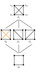
(a)

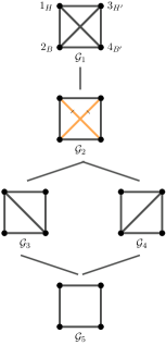
(b)

Figure 2: Frets’ Heads example: Comparison of the Hasse diagrams of two sublattices induced by the same five PD-CGs under (a) the model inclusion order, and (b) the twin order.

It is not difficult to use the result of Proposition 5 to generalise this idea to any set of neighbouring submodels. It follows that, in the implementation of the principle of coherence by using the twin lattice, the general rule is the same as in the model inclusion lattice: if a model is rejected then all the models in the paths descending from it should be excluded from the set of candidate models. In addition, there are specific rules for upper-layer models. If an upper-layer model is rejected then all the lower-layer models directly linked to it cannot be excluded from the candidate models. On the other hand, if it is accepted, one can exclude all the lower-layer models directly linked to it, and this can greatly reduce the number of candidate models, as shown by the simulations in Section 7.1.

It is also worth recalling that, in lattice theory, the sublattice of Figure 2(a) is said to have the diamond structure, and its presence in a the Hasse diagram causes the model inclusion lattice to be non-distributive (see Davey and Priestley, 2002, Theorem 4.10). The organization of the neighobouring submodels into the two-layer structure, provided by the twin lattice, is thus useful in the implementation of the coherence principle, but it has also the advantage of eliminating the diamond structure, thereby making the lattice distributive. The twin lattice seems therefore to represent the natural structure for the exploration of PD-RCON model spaces.

6 A coherent greedy search procedure

We introduce here a stepwise backward elimination procedure that exploits the twin lattice both for the computation of the meet operation and the implementation of the coherence principle.

Algorithm 1 Coherent stepwise backward elimination procedure

1:$\mathcal{G}^{\mbox{\footnotesize best}}\leftarrow$ complete graph with all colour classes atomic

2:$\mathcal{A}\leftarrow\emptyset$

3:$K\leftarrow$ maximum number of steps

4:$k\leftarrow 1$

5:for all upper-layer neighbouring submodels $\mathcal{H}$ of $\mathcal{G}^{\mbox{\footnotesize best}}$ do

6:     if $\mathcal{H}$ is accepted then $\mathcal{A}\leftarrow\mathcal{A}\cup\{\mathcal{H}\}$

7:end for

8:for all lower-layer neighbouring submodels $\mathcal{H}$ of $\mathcal{G}^{\mbox{\footnotesize best}}$ which are $\preceq_{t}$–incomparable with

9: for allevery graph in $\mathcal{A}$ do

10:     if $\mathcal{H}$ is accepted then $\mathcal{A}\leftarrow\mathcal{A}\cup\{\mathcal{H}\}$

11:end for

12:while $\mathcal{A}\neq\emptyset$ and $k<K$ do

13:     $\mathcal{A},\;\mathcal{G}^{\mbox{\footnotesize best}}\leftarrow\;$Update($\mathcal{A},\;\mathcal{G}^{\mbox{\footnotesize best}}$) $\triangleright$ see Algorithm 2

14:     $k\leftarrow k+1$

15:end while

16:if $\mathcal{A}\neq\emptyset$ and $k=K$ then $\mathcal{G}^{\mbox{\footnotesize best}}\leftarrow$ best model in $\mathcal{A}$

17:return $\mathcal{G}^{\mbox{\footnotesize best}}$

Every step of the procedure starts from a model, defined by a graph labelled as $\mathcal{G}^{\mbox{\footnotesize best}}$, and computes a set of candidate neighbouring submodels so as to obtain a set $\mathcal{A}$ of accepted models, according to a preestablished criterion. Specifically, we label as accepted the models with $p$-value of the likelihood ratio test against the saturated model, computed on the asymptotic chi-squared distribution, larger than $0.05$. Then a new $\mathcal{P}(\mathcal{G}^{\mbox{\footnotesize best}})$ is selected from $\mathcal{A}$. In this implementation, we choose as best model in $\mathcal{A}$ the model with largest $p$-value. We set the saturated model as starting point and then the procedure is iterated until either $\mathcal{A}$ is empty or a maximum number of iterations is reached. The pseudocode of the procedure is given in Algorithms 1 and 2 where, in order to make the code more readable, we have kept the technical level low. The pseudocode with all the technical details can be found in Algorithms 3 and 4 of the Supplementary Material.

An key issue concerns the identification, at every step, of the candidate models, which are all the coherent neighbouring submodels of $\mathcal{G}^{\mbox{\footnotesize best}}$. At the first step, efficiency is achieved by considering the upper layer first, and then the lower layer, so as to apply the principle of coherence as described in Section 5 and implemented in lines 5–11 of Algorithm 1. This can significantly reduce the dimension of the initial set of candidate models and, in turn, the dimension of the sets of candidate models of all the subsequent steps. In addition, the implementation of the coherence principle from the first step implies that the models in $\mathcal{A}$ are pairwise $\preceq_{t}$–incompatible and therefore, by Corollary 7, the next set of candidate models can be computed by using the more efficient $\wedge_{t}$ meet operation. Furthermore, Corollary 8 guarantees that the same can be done at every step of the procedure; see lines 14–17 of Algorithm 2.

Algorithm 2 Unpdate() procedure called by Algorithm 1

1:procedure Update($\mathcal{A},\;\mathcal{G}^{\mbox{\footnotesize best}}$)

2:     $\mathcal{G}^{\mbox{\footnotesize old}}\leftarrow\mathcal{G}^{\mbox{\footnotesize best}}$

3:     $\mathcal{G}^{\mbox{\footnotesize best}}\leftarrow$ best model in $\mathcal{A}$

4:     if $\mathcal{G}^{\mbox{\footnotesize best}}$ is obtained from $\mathcal{G}^{\mbox{\footnotesize old}}$ by removing exactly one edge $(i,j)$ with $i\neq\tau(j)$ then

5:         $\mathcal{H}\leftarrow$ graph obtained by removing from $\mathcal{G}^{\mbox{\footnotesize old}}$ the edge $\tau(i,j)$

6:         $\mathcal{A}\leftarrow\mathcal{A}\setminus\{\mathcal{H}\}$

7:     else if $\mathcal{G}^{\mbox{\footnotesize best}}$ is obtained from $\mathcal{G}^{\mbox{\footnotesize old}}$ by merging two atomic classes to obtain the

8:proelse iftwin-pairing class $\{(i,j),\tau(i,j)\}$ then

9:         $\mathcal{H}\leftarrow$ graph obtained by removing from $\mathcal{G}^{\mbox{\footnotesize old}}$ the edges $(i,j)$ and $\tau(i,j)$

10:         $\mathcal{A}\leftarrow\mathcal{A}\cup\{\mathcal{H}\}$

11:     end if

12:     $\mathcal{A^{\mbox{\footnotesize old}}}\leftarrow\mathcal{A}\setminus\{\mathcal{G}^{\mbox{\footnotesize best}}\}$

13:     $\mathcal{A}\leftarrow\emptyset$

14:     for all $\mathcal{F}\in\mathcal{A}^{\mbox{\footnotesize old}}$ do

15:         $\mathcal{H}\leftarrow\mathcal{F}\wedge_{t}\mathcal{G}^{\mbox{\footnotesize best}}$

16:         if $\mathcal{H}$ is accepted then $\mathcal{A}\leftarrow\mathcal{A}\cup\{\mathcal{H}\}$

17:     end for

18:     return $\mathcal{A}$ and $\mathcal{G}^{\mbox{\footnotesize best}}$

19:end procedure

7 Applications

7.1 Simulations

The greedy search procedure of the previous section has been implemented in the program language R, and here we analyse its behaviour on synthetic data. More specifically, we compare it with a stepwise backward elimination procedure that does not exploit the twin lattice for the computation of the set of candidate models, and where the principle of coherence is naively implemented by only considering the submodel relationship.

We considered two scenarios that differ for the sparsity degree, computed as $|E|/|F_{V}|$. For each of the two scenarios we generated four PD-CGs with $p=8,12,16,20$ and density degrees approximatively equal to $0.18$ for scenario $A$ and to $0.35$ for scenario $B$. Next, for every PD-CG $\mathcal{G}$ we randomly generated a concentration matrix $\Theta$ such that the normal distribution $N(0,\Theta^{-1})\in\mathcal{P}(\mathcal{G})$ and, finally, we randomly selected $20$ samples of size $100$ from such normal distribution; see Section S-5.1 of the Supplementary Material for details.

For each of the 160 synthetic datasets so generated, we ran the two greedy search procedures, which always terminated before the maximum number of iterations was reached. The performance of the two procedures is summarized in Table S-2 of the Supplementary Material. The point of main interest is the comparison in term of efficiency, that we quantify with respect to the average execution time and the average number of fitted models. These can be found in the last two columns of Table S-2 and, furthermore, the growth rates of these measurements are displayed in Figures 3 and 4. We can see that the procedure on the twin lattice is considerably more efficient. Specifically, the procedure on the twin lattice was more than five times faster, requiring between $16\%$ and $20\%$ of the time required by the procedure on the model inclusion lattice. Furthermore, the proper implementation of the coherence principle allowed us to fit a much smaller number of models, ranging between $37\%$ and $54\%$ of the models fitted under the naive implementation of principle of coherence. It is also interesting to notice that the latter proportions appear to decrease as $p$ increases. Table S-2 also gives the average values over the 20 samples of the positive predicted value, the true-positive rate and the true-negative rate, both for the edges and for the colour classes of the selected graphs. These have satisfying values and there are not relevant differences between the two procedures, thereby showing that the increase in efficiency is not achieved at the cost of a lower level of performance of the selected model.

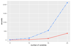
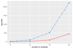
Figure 3: Average computational time in the simulations for the procedures based on the twin lattice (full red line) and on the model inclusion lattice (dashed blue line), for scenario A (left panel) and B (right panel).

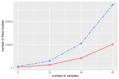
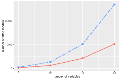
Figure 4: Averaged numbers of fitted models in the simulations for the procedures based on the twin lattice (full red line) and on the model inclusion lattice (dashed blue line), for scenario A (left panel) and B (right panel).

7.2 Brain networks from fMRI data

Functional MRI is a non invasive technique for collecting data on brain activity that measures the increase in the oxygenation level at some specific brain region, as long as an increase in blood flow occurs, due to some brain activity. The construction of a network from fMRI data requires first the identification of a set of functional vertices, such as spatial regions of interest (ROIs), and then the analysis of connectivity patterns across ROIs. The dataset we use for this application comes from a pilot study of the Enhanced Nathan Kline Institute-Rockland Sample project that are time series recorded on $70$ ROIs at $404$ equally spaced time. A detailed description of the project, scopes, and technical aspects can be found at http://fcon_1000.projects.nitrc.org/indi/enhanced/. Following Ranciati et al. (2021) we apply our method to the residuals estimated from the vector autogression models, carried out to remove the temporal dependence. We consider two subjects indexed by $14$ and $15$, who have the same psychological traits with no neuropsychiatric diseases and right-handedness. The main difference is that subject $14$ is $19$ years old whereas the subject $15$ is $57$ years old.

The human brain has a natural symmetric structure so that for every spatial ROI on the left hemisphere there is an homologous ROI on the right hemisphere. Accordingly, we identify the left and right groups with the left and the right hemispheres, respectively, and consider $36$ cortical brain regions, that are $22$ regions in the frontal lobe and $14$ regions in the anterior temporal lobe. We have therefore $|V|=36$ with $|L|=|R|=18$.

This section describes the analysis for the subject $15$ whereas the analysis of subject $14$ is given in Section S-5.2 of the Supplementary Material. We applied the procedure of Section 6 and selected the model defined by the PD-CG given in Figure 5. The graph of the selected model, denoted by $\mathcal{G}$, has density equal to $52.2\%$, the number of edges is 329 and there are $5$ vertex and $85$ edge twin-pairing colour classes, respectively. It provides an adequate fit with a $p$-value$=0.064$, computed on the asymptotic chi-squared distribution on 275 degrees of freedom of the likelihood ratio test for the comparison with the saturated model.

Note that Figure 5 splits the selected graph into 4 panels. The top-left panel gives the edges of $\mathcal{G}$ that belong to $E_{L}$ and form atomic colour classes, and similarly for the top-left panel that gives the atomic colour classes in $E_{R}$. Furthermore, the bottom-left and right panels give the edge twin-pairing colour classes between and across groups, respectively. We use the gray colour for both vertex and edge twin-pairing classes and, finally, we have omitted to represent the edges in $E_{T}$ because this set is almost complete, in the sense that $E_{T}=F_{T}\setminus\{(L4,R4)\}$. We deem that this representation can effectively illustrate the main features of the model, for example highlighting a high degree of symmetry in $\mathcal{G}$, given that $51.67\%$ of the edges of $\mathcal{G}$ belong to twin-pairing classes. The selected model has $275$ parameters and it is considerably more parsimonious than the saturated model that has $666$ parameters. It is also interesting to notice that the GGM defined by the undirected version of $\mathcal{G}$ has $90$ parameters more than the selected PD-RCON model.

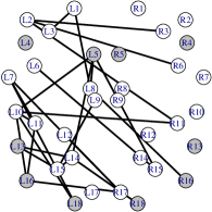
(a)

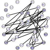
(b)

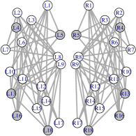
(c)

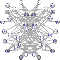
(d)

Figure 5: Selected PD-CG for subject 15 with separate panels for: (a) edges in $E_{L}$ forming atomic classes; (b) edges in $E_{R}$ forming atomic classes; (c) twin-pairing classes between groups; (d) twin-pairing classes across groups. Twin-pairing classes are depicted in gray, also for vertices, and the edges in $E_{T}$ are not depicted.

8 Conclusions

We have considered the problem of structure learning of GGMs for paired data by focusing on the family of RCON models defined by coloured graphs named PD-CGs. The main results of this paper provide insight into the structure of the model inclusion lattice of PD-CGs. We have introduced an alternative representation of these graphs that facilitates the computation of neighbouring models. Furthermore, this alternative representation is naturally associated with a novel order relationship that has lead to the construction of the twin lattice, whose structure resembles that of the well-known set inclusion lattice, and that facilitates the exploration of the search space. These results can be applied in the implementation of both greedy and Bayesian model search procedures. Here, we have shown how they can be used to improve the efficiency of stepwise backward elimination procedures. This has also made it clear that the use of the twin lattice facilitates the correct application of the principle of coherence. Finally, we have applied our procedure to learn a brain network on 36 variables. This model dimension could be regarded as somehow small, compared with other common nowadays applications of graphical models. However, as shown in Section 5, the number of PD-RCON models is much larger then that of GGMs and, as explained in Section 2.3, the application of penalized likelihood methods in paired data problems is problematic when variables do not have the same variance. Furthermore, the range of applications of our results do not restrict to PD-RCON models. In fact, the colouring of vertices and edges of PD-CGs can be associated with different types of equality restrictions, and thus to other types of graphical models for paired data for which penalized likelihood methods are not available. For instance, they could be used to identify a subfamily of RCOR models, which impose equality restrictions between specific partial variances and correlations (Højsgaard and Lauritzen, 2008). Further efficiency improvements are object of current research and could be achieved, for instance, by both implementing a procedure that deals with candidate submodels in parallel, and a procedure for the computation of maximum likelihood estimates explicitly designed for PD-RCON models.

Supplemental Materials for “Exploration of the search space of
Gaussian graphical models for paired data”

S-1 On the partition of the edge set induced by the twin-pairing function

In this section we provide a detailed example of the partition of the edge set of an undirected graph $G=(V,E)$ as described in Section 4.1 of the main paper. We let $p=6$ so that $V=\{1,2,3,4,5,6\}$ and, furthermore, we set $L=\{1,2,3\}$. Hence, $R=\{4,5,6\}$ and we assume that $\tau(i)=3+i$, for every $i\in L$, so that $\tau(1)=4$, $\tau(2)=5$ and $\tau(3)=6$.

In this case, the edge set of the complete graph is $F_{V}=\{(i,j)\mid i,j=1,\ldots,6;\;i<j\}$, and it can be partitioned into the three sets $F_{L}$, $F_{R}$ and $F_{T}$ as follows,

$$F_{L} = \{(1,2),(1,3),(2,3),(1,5),(1,6),(2,6)\},$$

$$F_{R} = \{(4,5),(4,6),(5,6),(2,4),(3,4),(3,5)\},$$

$$F_{T} = \{(1,4),(2,5),(3,6)\},$$

which are graphically represented in Figure S-1.

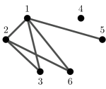
(a)

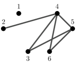
(b)

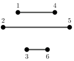
(c)

Figure S-1: Graphs with vertex set $V=\{1,2,3,4,5,6\}$ and edge sets: (a) $F_{L}$, (b) $F_{R}$ and (c) $F_{T}$.

Note that one can easily check that $F_{R}=\tau(F_{L})$, $F_{L}=\tau(F_{R})$ and $F_{T}=\tau(F_{T})$. In order to understand the meaning of this partition of $F_{V}$ it is useful to note that the set $F_{L}$ can be seen as the union of two disjoint subsets, $F_{L}=F_{L}^{(within)}\cup F_{L}^{(across)}$ where

$$F_{L}^{(within)} = \{(i,j)\in F_{V}\mid i,j\in L\}$$

$$F_{L}^{(across)} = \{(i,j)\in F_{V}\mid i\in L,j\in R,i<\tau(j)\}.$$

Dually, $F_{R}=F_{R}^{(within)}\cup F_{R}^{(across)}$ with

$$F_{R}^{(within)} = \{(i,j)\in F_{V}\mid i,j\in R\}$$

$$F_{R}^{(across)} = \{(i,j)\in F_{V}\mid i\in L,j\in R,i>\tau(j)\}.$$

Note that $F_{L}^{(within)}=\tau(F_{R}^{(within)})$ and thus $F_{R}^{(within)}=\tau(F_{L}^{(within)})$, so that every edge in $F_{L}^{(within)}$ has a twin in $F_{R}^{(within)}$. The edges in $F_{L}^{(within)}$ and $F_{R}^{(within)}$ belong to the left and right group, respectively, and thus the twin-pairing classes characterized by these edges encode similarities involving edges within the two groups. For the example on $p=6$ these two sets become $F_{L}^{(within)}=\{(1,2),(1,3),(2,3)\}$ and $F_{R}^{(within)}=\{(4,5),(4,6),(5,6)\}$ and the relevant twin-pairing classes are represented in Figure S-2.

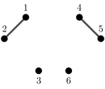
(a)

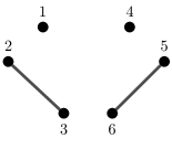
(b)

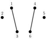
(c)

Figure S-2: Edge twin-pairing classes involving edges within groups: each of the graphs (a), (b) and (c) contains exactly one edge $(i,j)\in F_{L}^{(within)}=\{(1,2),(1,3),(2,3)\}$ and its twin $\tau(i,j)\in F_{R}^{(within)}=\{(4,5),(4,6),(5,6)\}$.

The edges in $F_{L}^{(across)}$ and $F_{R}^{(across)}$ encode the cross-group association structure. Also in this case $F_{L}^{(across)}=\tau(F_{R}^{(across)})$ and $F_{T}^{(across)}=\tau(F_{T})^{(across)}$ so that every edge in $F_{L}^{(across)}$ has a twin in $F_{R}^{(across)}$. For the case $p=6$ these sets become $F_{L}^{(across)}=\{(1,5),(1,6),(2,6)\}$ and $F_{R}^{(across)}=\{(2,4),(3,4),(3,5)\}$ and the corresponding colour classes are depicted in Figure S-3.

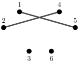
(a)

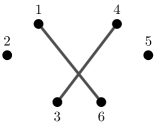
(b)

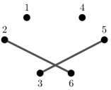
(c)

Figure S-3: Edge twin-pairing classes involving edges across groups: each of the graphs (a), (b) and (c) contains exactly one edge $(i,j)\in F_{L}^{(across)}=\{(1,5),(1,6),(2,6)\}$ and its twin $\tau(i,j)\in F_{R}^{(across)}=\{(2,4),(3,4),(3,5)\}$.

Consider now the PD-CG in Figure S-4. This is denoted by $\mathcal{G}=(\mathcal{V},\mathcal{E})$ with

$$\mathcal{V} = \{\{1,4\},\{2,5\},\{3\},\{6\}\}$$

$$\mathcal{E} = \{\{(1,2),(4,5)\},\{(1,4)\},\{(1,6)\},\{(2,3)\},\{(3,4)\},\{(3,5)\}\}.$$

We now compute the equivalent representation $\mathcal{G}=(V,E,\mathbb{L},\mathbb{E})$. First, we can trivially obtain that $V=\{1,2,3,4,5,6\}$ and $E=\{(1,2),(1,4),(1,6),(2,3),(3,4),(3,5),(4,5)\}$. Next, because $L=\{1,2,3\}$ and the only vertex atomic colour classes are $\{3\}$ and $\{6\}$, we can see that $\mathbb{L}=\{3\}$. Finally, we compute $E_{L}=E\cap F_{L}=\{(1,2),(1,6),(2,3)\}$ and $E_{R}=E\cap F_{R}=\{(4,5),(3,4),(3,5)\}$. It follows that $\tau(E_{R})=\{(1,2),(1,6),(2,6)\}$ so that $E_{L}\cap\tau(E_{R})=\{(1,2),(1,6)\}$. Because the edge $(1,2)$ belongs to a twin-pairing colour class with its twin $(4,5)$, whereas $(1,6)$ belongs to an atomic colour class, then we obtain that $\mathbb{E}=\{(1,6)\}$.

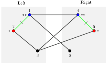
Figure S-4: Example of coloured graph for paired data.

S-2 An example of neighbouring-submodel two layer structure

In this example, we consider a set of neighbouring submodels and compare their relationships under the model inclusion and the twin order. To this aim, we describe the structure of a portion of the Hasse diagram of the PD-RCON models with $p=4$ and, more specifically, Figure S-5 shows the model inclusion lattice of PD-RCON models in the Frets’ heads example, where the model on the top is the saturated model that is then linked to its neighbouring submodels, represented by the coloured graphs on the highlighted area. On the other hand, Figure S-6 presents the twin lattice of the same models, that refines the model inclusion lattice into the two-layer structure so that every model in the lower layer is $\preceq_{t}$–smaller than some models in the upper, and within each layer, models are pairwise both $\preceq_{s}$– and $\preceq_{t}$–incomparable.

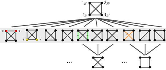
Figure S-5: Part of the Hasse diagram of the model inclusion lattice for the Frets’ heads example. The graph representing the saturated model is depicted on the top and followed, below, by the graphs representing its neighbouring submodels, which on the highlighted area. Then two graphs of the third level are given.

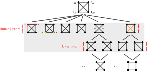
Figure S-6: Part of the Hasse diagram of the twin lattice for the Frets’ heads example. The graph representing the saturated model is depicted on the top. The graphs on the highlighted area are those representing the model inclusion neighbouring submodels of the saturated model, which are organized in a two-layer structure, to be compared with Figure S-5.

S-3 Dimensions of the search space of PD-RCON models

In this section, we provide a formula for the computation of the number of PD-RCON models $\mathcal{P}(V)$ with $|V|=p$.

Firstly, we notice that in a PD-RCON model with $p$ variables the maximum numbers of vertex and edge twin-pairing colour classes are $p/2$ and $|F_{L}|=p(p-2)/4$, respectively. Next, we compute $|\mathcal{P}(V)|$ by steps, starting from the case where there are no twin-pairing colour classes and then increasing the number of twin-twin pairing classes.

• the number of PD-CGs where all colour classes are atomic coincides with the number of GGMs and is equal to $2^{p\choose 2}$,

• the number of PD-CGs where vertex twin-pairing classes are allowed but edge colour classes are all atomic is $2^{p/2}\times 2^{\binom{p}{2}}$,

• the number of PD-CGs where vertex twin-pairing classes are allowed and at most $1$ edge twin-pairing class is present is

  $$2^{p/2}\binom{p(p-2)/4}{1}2^{\binom{p}{2}-2},$$

• the number of PD-CGs where vertex twin-pairing classes are allowed and at most $2$ edge twin-pairing classes are present is

  $$2^{p/2}\binom{p(p-2)/4}{2}2^{\binom{p}{2}-4},$$

• the number of PD-CGs where vertex twin-pairing classes are allowed and at most $i$ edge twin-pairing classes are present, with $0\leq i\leq p(p-2)/4$, is

  $$2^{p/2}\binom{p(p-2)/4}{i}2^{\binom{p}{2}-2i}.$$

So finally, the number of PD-RCON models is

$$|\mathcal{P}(V)|=2^{p/2}\sum_{i=0}^{p(p-2)/4}\binom{p(p-2)/4}{i}2^{\binom{p}{2}-2i}.$$

S-4 Technical details on the greedy search procedure

Here we provide Algorithms 3 and 4 which contain a fully detailed, expanded, version of the pseudocode given in Algorithms 1 and 2 of the main paper. Note that the pseudocode calls the procedures Is.Accepted() and Best.Model() that are left unspecified. The procedure Is.Accepted() takes a model as input and returns true is the model satisfies a given, arbitrary, criterium and false otherwise. The procedure Best.Model() accepts a non-empty set of models as input and returns one of the models of such set that is identified as “best”, according to a specified criterium. Finally, an implementation of the procedure in the programming language R can be found at https://github.com/NgocDung-NGUYEN/backwardCGM-PD.

Algorithm 3 Expanded version of the pseudocode in Algorithm 1 of the main paper.

1:$V$ and $L$

2:$\mathcal{G}^{\mbox{\footnotesize best}}\leftarrow(V,F_{V},L,F_{L})$

3:$\mathcal{A}\leftarrow\emptyset$

4:$K\leftarrow$ maximum number of steps ($\geq 1)$

5:$k\leftarrow 1$

6:for all $i\in L$ do

7:     $\mathcal{H}\leftarrow(V,F_{V},L\setminus\{i\},F_{L})$

8:     if Is.Accepted($\mathcal{H}$) then

9:         $\mathcal{A}\leftarrow\mathcal{A}\cup\{\mathcal{H}\}$

10:     end if

11:     $\mathcal{H}\leftarrow(V,F_{V}\setminus\{(i,\tau(i))\},L,F_{L})$

12:     if Is.Accepted($\mathcal{H}$) then

13:         $\mathcal{A}\leftarrow\mathcal{A}\cup\{\mathcal{H}\}$

14:     end if

15:end for

16:for all $(i,j)\in F_{L}$ do

17:     $\mathcal{H}\leftarrow(V,F_{V},L,F_{L}\setminus\{(i,j)\})$

18:     if Is.Accepted($\mathcal{H}$) then

19:         $\mathcal{A}\leftarrow\mathcal{A}\cup\{\mathcal{H}\}$

20:     else

21:         $\mathcal{H}\leftarrow(V,F_{V}\setminus\{(i,j)\},L,F_{L}\setminus\{(i,j)\})$

22:         if Is.Accepted($\mathcal{H}$) then

23:              $\mathcal{A}\leftarrow\mathcal{A}\cup\{\mathcal{H}\}$

24:         end if

25:         $\mathcal{H}\leftarrow(V,F_{V}\setminus\{\tau(i,j)\},L,F_{L}\setminus\{(i,j)\})$

26:         if Is.Accepted($\mathcal{H}$) then

27:              $\mathcal{A}\leftarrow\mathcal{A}\cup\{\mathcal{H}\}$

28:         end if

29:     end if

30:end for

31:while $\mathcal{A}\neq\emptyset$ and $k<K$ do

32:     $\mathcal{A},\;\mathcal{G}^{\mbox{\footnotesize best}}\leftarrow\;$Update($\mathcal{A},\;\mathcal{G}^{\mbox{\footnotesize best}}$) $\triangleright$ see Algorithm 4

33:     $k\leftarrow k+1$

34:end while

35:if $\mathcal{A}\neq\emptyset$ and $k=K$ then $\mathcal{G}^{\mbox{\footnotesize best}}\leftarrow$Best.Model($\mathcal{A}$)

36:return $\mathcal{G}^{\mbox{\footnotesize best}}$

Algorithm 4 Expanded version of the pseudocode in Algorithm 2 of the main paper.

1:procedure Update($\mathcal{A},\;\mathcal{G}^{\mbox{\footnotesize best}}$)

2:     $\mathcal{G}^{\mbox{\footnotesize old}}\leftarrow\mathcal{G}^{\mbox{\footnotesize best}}$

3:     $\mathcal{G}^{\mbox{\footnotesize best}}\leftarrow$Best.Model($\mathcal{A}$) $\triangleright$ Note that: $\mathcal{G}^{\mbox{\footnotesize old}}=(V,E^{\mbox{\footnotesize old}},\mathbb{L}^{\mbox{\footnotesize old}},\mathbb{E}^{\mbox{\footnotesize old}})$ $\mathcal{G}^{\mbox{\footnotesize best}}=(V,E^{\mbox{\footnotesize best}},\mathbb{L}^{\mbox{\footnotesize best}},\mathbb{E}^{\mbox{\footnotesize best}})$

4:     $e\leftarrow E^{\mbox{\footnotesize best}}\setminus E^{\mbox{\footnotesize old}}$

5:     if $|e|=1$ and $e\neq\tau(e)$ then

6:         $\mathcal{H}\leftarrow(V,E^{\mbox{\footnotesize old}}\setminus\{\tau(e)\},\mathbb{L}^{\mbox{\footnotesize old}},\mathbb{E}^{\mbox{\footnotesize old}}\setminus\{e,\tau(e)\})$

7:         $\mathcal{A}\leftarrow\mathcal{A}\setminus\{\mathcal{H}\}$

8:     else if $e=\emptyset$ and $\mathbb{E}^{\mbox{\footnotesize best}}\neq\mathbb{E}^{\mbox{\footnotesize old}}$ then

9:         $e\leftarrow\mathbb{E}^{\mbox{\footnotesize old}}\setminus\mathbb{E}^{\mbox{\footnotesize best}}$

10:         $\mathcal{H}\leftarrow(V,E^{\mbox{\footnotesize old}}\setminus\{e,\tau(e)\},\mathbb{L}^{\mbox{\footnotesize old}},\mathbb{E}^{\mbox{\footnotesize old}}\setminus\{e\})$

11:         $\mathcal{A}\leftarrow\mathcal{A}\cup\{\mathcal{H}\}$

12:     end if

13:     $\mathcal{A^{\mbox{\footnotesize old}}}\leftarrow\mathcal{A}\setminus\{\mathcal{G}^{\mbox{\footnotesize best}}\}$

14:     $\mathcal{A}\leftarrow\emptyset$

15:     for all $\mathcal{F}\in\mathcal{A}^{\mbox{\footnotesize old}}$ do

16:         $\mathcal{H}\leftarrow\mathcal{F}\wedge_{t}\mathcal{G}^{\mbox{\footnotesize best}}$

17:         if Is.Accepted($\mathcal{H}$) then $\mathcal{A}\leftarrow\mathcal{A}\cup\{\mathcal{H}\}$

18:     end for

19:     return $\mathcal{A}$ and $\mathcal{G}^{\mbox{\footnotesize best}}$

20:end procedure

S-5 Additional details on the applications

S-5.1 Simulations

In this section, we provide additional details on the simulations described in Section 7.1 on the main paper; see also https://github.com/NgocDung-NGUYEN/backwardCGM-PD.

Table S-1 considers the 8 PD-CGs used in the simulations and gives details on edges, pairs of twin edges present in the graph and colour classes.

Table S-1: Details on the PD-CGs used in the simulations: den._% is the density computed from $|E|/|F_{V}|$; $|E|$ is the number of edges; $|E_{T}|$ is the number of edges connecting pairs of twin vertices; $|E_{L}\cap\tau(E_{R})|$ is the number of edges for which a twin is present in the graph; $|\mathbb{E}|$ and $|\mathbb{L}|$ are the number of edge and vertex atomic colour classes, respectively; $|\mathbb{E}^{c}|=|(E_{L}\cap\tau(E_{R}))\setminus\mathbb{E}|$ and $|\mathbb{L}^{c}|=|L\setminus\mathbb{L}|$ are the number of edge and vertex twin-pairing classes, respectively.

$p$	Scen.	Structure					Symmetries
		den.%	$|E|$	$|E_{T}|$	$|E_{L}\cap\tau(E_{R})|$		$|\mathbb{E}|$	$|\mathbb{E}^{c}|$	$|\mathbb{L}|$	$|\mathbb{L}^{c}|$
$8$	A	$17.85$	$5$	$0$	$2$		$1$	$1$	$3$	$1$
	B	$35.71$	$10$	$0$	$4$		$1$	$3$	$1$	$3$
$12$	A	$18.18$	$12$	$0$	$5$		$4$	$1$	$4$	$2$
	B	$34.85$	$23$	$1$	$9$		$3$	$6$	$2$	$4$
$16$	A	$18.33$	$22$	$1$	$9$		$7$	$2$	$6$	$2$
	B	$35.00$	$42$	$3$	$15$		$5$	$10$	$2$	$6$
$20$	A	$17.94$	$34$	$2$	$14$		$11$	$3$	$8$	$2$
	B	$34.74$	$66$	$6$	$24$		$8$	$16$	$2$	$8$

For each PD-CG in Table S-1 above, we generated a concentration matrix by exploiting the R package gRc (Højsgaard et al., 2007). More specifically, we applied the function rcox() by giving in input the $p\times p$ equicorrelation matrix with the diagonal entries equal to $1$, and all off-diagonal entries equal to $0.5$. Each of resulting concentration matrices was used to generate $20$ random samples of size $n=100$ from the relevant multivariate normal distribution, with mean vector equal to zero. The two procedures were then applied to the $20\times 8=160$ datasets so obtained, and we also remark that we exploited the package gRc for the computation of maximum likelihood estimates.

Table S-2 summarizes the average results over all repetitions of the simulated data of the performance scores which measure the identifications of the zeros and symmetric structures of the resulting models recovered from the model selection procedure. Specifically, for the accuracy of the graph structures, we considered the quantities such as the edge positive-predicted value (ePPV), the edge true-positive rate (eTPR), and the edge true-negative rate (eTNR), which are formally specified as

$$\operatorname*{ePPV}=\frac{\operatorname*{eTP}}{\#\text{edges}},\quad\operatorname*{eTPR}=\frac{\operatorname*{eTP}}{\operatorname*{eP}},\quad\operatorname*{eTNR}=\frac{\operatorname*{eTN}}{\operatorname*{eN}},$$

where

• eTP: the number of true edges in the selected graph,

• $\#$edges: the number of edges in the selected graph,

• eP: the number of edges in the true graph,

• eTN: the number of true missing edges in the selected graph,

• eN: the number of missing edges in the true graph.

Similarly, for the identification of the symmetries, that is of the twin-pairing classes, we considered the symmetry positive-predicted value (sPPV), the symmetry true-positive rate (sTPR), and the symmetry true-negative rate (sTNR), as defined by Ranciati et al. (2021). Specifically, they are computed as

$$\operatorname*{sPPV}=\frac{\operatorname*{sTP}}{\#\text{sym}},\quad\operatorname*{sTPR}=\frac{\operatorname*{sTP}}{\operatorname*{sP}},\quad\operatorname*{sTNR}=\frac{\operatorname*{sTN}}{\operatorname*{sN}},$$

where

• sTP: the number of pairs of true twin-pairing edges in the selected graph,

• $\#$sym: the number of pairs of twin-pairing edges in the selected graph,

• sP: the number of pairs of twin-pairing edges in the true graph,

• sTN:the number of pairs of twin-pairing edges that are missing in the selected graph,

• sN: the number of pairs of twin-pairing edges that are missing in the true graph.

Finally, on the last two columns of the table we report the computational time of the procedures and the total number of fitted models during the execution of the algorithms.

Table S-2: Performance measures of the model selection procedures on the lattice structures ordered by $\preceq_{t}$ and $\preceq_{s}$. Results are recorded as mean computed across the $20$ replicated datasets for each scenario. Here, the columns of $\#$edges and $\#$sym include the average numbers of edges and of pairs of symmetric edges, respectively, and the numbers in the round bracket are the corresponding standard deviations. The columns of Time and $\#$models measure the efficiency of the procedures that are the average of computational time and the average of numbers of fitted models, respectively.

S	$p$	Order	Graph structure					Symmetries				Time${}_{\text{(s)}}$	$\#$models
			$\#$edges	ePPV%	eTPR%	eTNR%		$\#$sym	sPPV%	sTPR%	sTNR%
A	$8$	$\preceq_{t}$	$7(2)$	$76.68$	$100.00$	$91.52$		$2(1)$	$41.67$	$95.00$	$89.44$	$4$	$273$
		$\preceq_{s}$	$7(2)$	$75.41$	$100.00$	$91.30$		$2(1)$	$46.67$	$95.00$	$85.56$	$17$	$580$
	$12$	$\preceq_{t}$	$17(3)$	$71.22$	$97.92$	$90.37$		$6(1)$	$15.99$	$90.00$	$87.61$	$19$	$1300$
		$\preceq_{s}$	$17(3)$	$70.23$	$98.75$	$90.00$		$5(1)$	$17.34$	$90.00$	$83.91$	$109$	$2985$
	$16$	$\preceq_{t}$	$27(4)$	$74.83$	$88.64$	$92.70$		$9(1)$	$18.53$	$85.00$	$89.43$	$89$	$4245$
		$\preceq_{s}$	$28(4)$	$70.98$	$87.05$	$91.48$		$8(1)$	$19.32$	$77.50$	$84.77$	$532$	$10554$
	$20$	$\preceq_{t}$	$44(8)$	$64.24$	$82.21$	$89.49$		$16(3)$	$13.47$	$70.00$	$86.18$	$379$	$10212$
		$\preceq_{s}$	$46(7)$	$60.11$	$78.97$	$88.04$		$13(3)$	$11.97$	$51.67$	$80.00$	$2102$	$27356$
B	$8$	$\preceq_{t}$	$11(2)$	$84.54$	$89.50$	$89.72$		$5(1)$	$64.08$	$93.33$	$92.50$	$4$	$264$
		$\preceq_{s}$	$11(2)$	$83.59$	$89.00$	$89.44$		$4(1)$	$64.83$	$85.00$	$85.83$	$15$	$486$
	$12$	$\preceq_{t}$	$23(4)$	$81.78$	$80.00$	$89.65$		$9(2)$	$56.28$	$79.17$	$87.35$	$19$	$1230$
		$\preceq_{s}$	$23(4)$	$81.25$	$78.48$	$89.53$		$7(2)$	$63.26$	$73.33$	$83.53$	$102$	$2729$
	$16$	$\preceq_{t}$	$34(5)$	$72.49$	$57.86$	$87.63$		$12(2)$	$52.38$	$64.00$	$86.09$	$96$	$4259$
		$\preceq_{s}$	$31(4)$	$74.50$	$55.24$	$89.49$		$9(2)$	$63.36$	$54.00$	$82.97$	$523$	$10247$
	$20$	$\preceq_{t}$	$51(9)$	$69.74$	$53.41$	$87.02$		$18(2)$	$48.17$	$54.38$	$84.07$	$452$	$10300$
		$\preceq_{s}$	$48(7)$	$67.81$	$48.64$	$87.22$		$12(2)$	$52.97$	$39.38$	$78.98$	$2226$	$26961$

S-5.2 Additional details on the application to fMRI data

We applied our method to a multimodal imaging dataset coming from a pilot study of the Enhanced Nathan Kline Institute-Rockland Sample project, and provided by Greg Kiar and Eric Bridgeford from NeuroData at Johns Hopkins University, who pre-processed the raw DTI and R-fMRI imaging data available at http://fcon_1000.projects.nitrc.org/indi/CoRR/html/nki_1.html, using the pipelines ndmg and C-PAC. Particularly, the R-fMRI monitors brain functional activity at different regions via dynamic changes in the blood oxygenation level depedent (BOLD) signal, when, in this study, the subjects are simply asked to stay awake with eyes open. The data sets that we apply our methods are residuals estimated from the vector autogression models carried out to remove the temporal dependence, see Ranciati et al. (2021).

We considered $36$ cortical brain regions including $22$ regions in the frontal lobe and $14$ regions in the anterior temporal lobe for two subjects 14 and 15. In this section, we provide the analysis of subject 14 while the analysis of subject 15 is given in the main paper. In particular, the graph of the selected model by our method, called by $\mathcal{G}$, has density equal to $54.28\%$ with $342$ edges present in which there are $76$ edge twin-pairing colour classes, which to make up approximately $44.44\%$ on present edges, and $6$ vertex twin-pairing colour classes. Based on the likelihood ratio test for the comparison with the saturated model, the model $\mathcal{G}$ has $p$-values equal to $0.055$ with $296$ degrees of freedom computed on the asymptotic chi-squared distribution.

Figure S-7 presents the coloured graphical representation of the model $\mathcal{G}$ that is split into $4$ panels. The top-left panel gives the edges of $\mathcal{G}$ that belong to $E_{L}$ and form atomic colour classes, and similarly for the top-left panel that gives the atomic colour classes in $E_{R}$. Furthermore, the bottom-left and right panels give the edge twin-pairing colour classes between and across groups, respectively. Here, in this case, we have omitted to represent the edges in $E_{T}$ because this set is complete, in the sense that $E_{T}=F_{T}$.

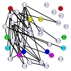
(a)

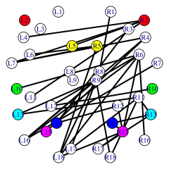
(b)

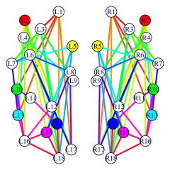
(c)

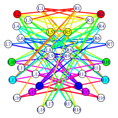
(d)

Figure S-7: The PD-CG of the selected models for subject $14$ with separate panels: (a) edges in $E_{L}$ forming atomic classes; (b) edges in $E_{R}$ forming atomic classes; (c) twin-pairing classes within groups; and (d) twin pairing classes across groups.

S-6 Proofs

S-6.1 Proof of Proposition 1

We now show that from the quadruplet $(V,E,\mathbb{L},\mathbb{E})$ obtained from (1) and (2) one can recover the representation $\mathcal{G}=(\mathcal{V},\mathcal{E})$ by applying (i) and (ii). Recall that every colour class of both $\mathcal{V}$ and $\mathcal{E}$ is either atomic or twin-pairing. We consider first the vertex colour classes $\mathcal{V}$. Every twin-pairing vertex colour class can be written as $\{i,\tau(i)\}$ with $i\in L$ and $\tau(i)\in R$, and it follows from the definition of $\mathbb{L}$ in (2) that a vertex $i\in L$ belongs to a twin-pairing colour class if and only if $i\in L\setminus\mathbb{L}$. Hence, from the pair $L$ and $\mathbb{L}$ we can obtain the twin-pairing colour classes in $\mathcal{V}$ which are the sets $\{i,\tau(i)\}$ for all $i\in L\setminus\mathbb{L}$. It is straightforward that all the vertices in $V$ not belonging to any of the above twin-pairing classes must form atomic colour classes. We now turn to the edge colour classes $\mathcal{E}$. The partition $(E_{L},E_{R},E_{T})$ of $E$ is obtained in such a way that every twin-pairing edge colour class can be written as $\{(i,j),\tau(i,j)\}$ with $(i,j)\in E_{L}$ and $\tau(i,j)\in E_{R}$ and therefore it holds that $(i,j)\in E_{L}\cap\tau(E_{R})$. Furthermore, by construction, the set $\mathbb{E}$ in (2) is made up of all the edges in $E_{L}\cap\tau(E_{R})$ which form atomic colour classes. It follows that the twin-pairing edge colour classes of $\mathcal{G}$ are given by the pairs $\{(i,j),\tau(i,j)\}$ for all $(i,j)\in(E_{L}\cap\tau(E_{R}))\setminus\mathbb{E}$, as required. Also in this case it is straightforward to see that all the edges in $E$ not belonging to any of the above twin-pairing classes must form atomic colour classes.

S-6.2 Proof of Theorem 2

Let $\mathcal{G}=(\mathcal{V},\mathcal{E})\in\mathcal{P}$ be a PD-CG and let $(V,E,\mathbb{L},\mathbb{E})$ the quadruplet obtained from the application of (1) and (2). It follows immediately from the construction of $G=(V,E)$ in (1) and of $\mathbb{L}$ and $\mathbb{E}$ in (2) that $(V,E,\mathbb{L},\mathbb{E})$ is compatible with $(L,R)$. Furthermore, the pair $(\mathcal{V},\mathcal{E})$ can be recovered from $(V,E,\mathbb{L},\mathbb{E})$ as shown in Proposition 1.

Consider now a compatible quadruplet $(V,E,\mathbb{L},\mathbb{E})$ and let $\mathcal{G}=(\mathcal{V},\mathcal{E})$ the graph obtained from the application of Proposition 1. It follows immediately from the constructing procedure that $\mathcal{G}\in\mathcal{P}$ and we have to show that if we apply (1) and (2) to $\mathcal{G}$ then we recover the quadruplet $(V,E,\mathbb{L},\mathbb{E})$. It is straightforward to see that (1) gives $V_{\mathcal{G}}=V$ and $E_{\mathcal{G}}=E$. By (i) of Proposition 1, the twin-pairing vertex colour classes of $\mathcal{G}$ are $\{i,\tau(i)\}$ for all $i\in L\setminus\mathbb{L}$ and therefore we obtain from (2) that $\mathbb{L}_{\mathcal{G}}=L\cap\mathbb{L}=\mathbb{L}$ because $\mathbb{L}\subseteq L$ by compatibility. Similarly, we obtain from (ii) of Proposition 1 and (2) that $\mathbb{E}_{\mathcal{G}}=(E_{L}\cap\tau(E_{R}))\cap\mathbb{E}=\mathbb{E}$ because $\mathbb{E}\subseteq E_{L}\cap\tau(E_{R})$ by compatibility. And this completes the proof.

S-6.3 Proof of Theorem 3

The proof of this theorem is as follows: we firstly prove that $\langle\mathcal{P},\preceq_{t}\rangle$ is a lattice by determining the explicit forms of the corresponding meet and join operations. We then identify the zero and the unit of the lattice $\langle\mathcal{P},\preceq_{t}\rangle$, which implies completeness. Finally, we prove that $\langle\mathcal{P},\preceq_{t}\rangle$ is distributive.

We first consider (i) and show that $\mathcal{L}=(V,E_{\mathcal{G}}\cap E_{\mathcal{H}},\mathbb{L}_{\mathcal{G}}\cap\mathbb{L}_{\mathcal{H}},\mathbb{E}_{\mathcal{G}}\cap\mathbb{E}_{\mathcal{H}})$ is the meet of $\mathcal{G}$ and $\mathcal{H}$, $\mathcal{G}\wedge_{t}\mathcal{H}$. It can be easily checked that, by construction, the quadruplet $(V,E_{\mathcal{G}}\cap E_{\mathcal{H}},\mathbb{L}_{\mathcal{G}}\cap\mathbb{L}_{\mathcal{H}},\mathbb{E}_{\mathcal{G}}\cap\mathbb{E}_{\mathcal{H}})$ is compatible so that $\mathcal{L}\in\mathcal{P}$. Furthermore, because $E_{\mathcal{G}}\cap E_{\mathcal{H}}\subseteq E_{\mathcal{G}}$, $\mathbb{L}_{\mathcal{G}}\cap\mathbb{L}_{\mathcal{H}}\subseteq\mathbb{L}_{\mathcal{G}}$ and $\mathbb{E}_{\mathcal{G}}\cap\mathbb{E}_{\mathcal{H}}\subseteq\mathbb{E}_{\mathcal{G}}$, then it follows immediately from Definition 3 that $\mathcal{L}\preceq_{t}\mathcal{G}$ and, similarly, one can show that $\mathcal{L}\preceq_{t}\mathcal{H}$, so that $\mathcal{L}\preceq_{t}\mathcal{G},\mathcal{H}$. In this way, we have shown that $\mathcal{L}$ is a lower bound of $\mathcal{G}$ and $\mathcal{H}$ and now, in order to prove that $\mathcal{L}=\mathcal{G}\wedge_{t}\mathcal{H}$, we have to show that $\mathcal{L}$ is the greatest lower bound, or infimum, of $\mathcal{G}$ and $\mathcal{H}$. More formally, we have to show that if $\mathcal{F}=(V,E_{\mathcal{F}},\mathbb{L}_{\mathcal{F}},\mathbb{E}_{\mathcal{F}})$ is an arbitrary lower bound of $\mathcal{G}$ and $\mathcal{H}$ then $\mathcal{F}\preceq_{t}\mathcal{L}$. For every lower bound $\mathcal{F}$ of $\mathcal{G}$ and $\mathcal{H}$ it holds that $\mathcal{F}\preceq_{t}\mathcal{G},\mathcal{H}$ and, therefore, that

1. both $E_{\mathcal{F}}\subseteq E_{\mathcal{G}}$ and $E_{\mathcal{F}}\subseteq E_{\mathcal{H}}$,

2. both $\mathbb{L}_{\mathcal{F}}\subseteq\mathbb{L}_{\mathcal{G}}$ and $\mathbb{L}_{\mathcal{F}}\subseteq\mathbb{L}_{\mathcal{H}}$,

3. both $\mathbb{E}_{\mathcal{F}}\subseteq\mathbb{E}_{\mathcal{G}}$ and $\mathbb{E}_{\mathcal{F}}\subseteq\mathbb{E}_{\mathcal{H}}$.

In turn, this implies that $E_{\mathcal{F}}\subseteq E_{\mathcal{G}}\cap E_{\mathcal{H}}$, $\mathbb{L}_{\mathcal{F}}\subseteq\mathbb{L}_{\mathcal{G}}\cap\mathbb{L}_{\mathcal{H}}$ and $\mathbb{E}_{\mathcal{F}}\subseteq\mathbb{E}_{\mathcal{G}}\cap\mathbb{E}_{\mathcal{H}}$ and therefore that $\mathcal{F}\preceq_{t}\mathcal{L}$, as required.

We now consider (ii) and show that $\mathcal{U}=(V,E_{\mathcal{G}}\cup E_{\mathcal{H}},\mathbb{L}_{\mathcal{G}}\cup\mathbb{L}_{\mathcal{H}},\mathbb{E}_{\mathcal{G}}\cup\mathbb{E}_{\mathcal{H}})$ is the join of $\mathcal{G}$ and $\mathcal{H}$, $\mathcal{G}\vee_{t}\mathcal{H}$. It can be easily checked that, by construction, the quadruplet $(V,E_{\mathcal{G}}\cup E_{\mathcal{H}},\mathbb{L}_{\mathcal{G}}\cup\mathbb{L}_{\mathcal{H}},\mathbb{E}_{\mathcal{G}}\cup\mathbb{E}_{\mathcal{H}})$ is compatible so that $\mathcal{U}\in\mathcal{P}$. Furthermore, because $E_{\mathcal{G}}\subseteq E_{\mathcal{G}}\cup E_{\mathcal{H}}$, $\mathbb{L}_{\mathcal{G}}\subseteq\mathbb{L}_{\mathcal{G}}\cup\mathbb{L}_{\mathcal{H}}$ and $\mathbb{E}_{\mathcal{G}}\subseteq\mathbb{E}_{\mathcal{G}}\cup\mathbb{E}_{\mathcal{H}}$, then it follows immediately from Definition 3 that $\mathcal{G}\preceq_{t}\mathcal{U}$ and, similarly, one can show that $\mathcal{H}\preceq_{t}\mathcal{U}$ so that $\mathcal{G},\mathcal{H}\preceq_{t}\mathcal{U}$. In this way, we have shown that $\mathcal{U}$ is an upper bound of $\mathcal{G}$ and $\mathcal{H}$ and now, in order to prove that $\mathcal{U}=\mathcal{G}\vee_{t}\mathcal{H}$, we have to show that $\mathcal{U}$ is the least upper bound, or supremum, of $\mathcal{G}$ and $\mathcal{H}$. More formally, we have to show that if $\mathcal{F}=(V,E_{\mathcal{F}},\mathbb{L}_{\mathcal{F}},\mathbb{E}_{\mathcal{F}})$ is an arbitrary upper bound of $\mathcal{G}$ and $\mathcal{H}$ then $\mathcal{U}\preceq_{t}\mathcal{F}$. For every upper bound $\mathcal{F}$ of $\mathcal{G}$ and $\mathcal{H}$ it holds that $\mathcal{G},\mathcal{H}\preceq_{t}\mathcal{F}$ and, therefore, that

1. both $E_{\mathcal{G}}\subseteq E_{\mathcal{F}}$ and $E_{\mathcal{H}}\subseteq E_{\mathcal{F}}$,

2. both $\mathbb{L}_{\mathcal{G}}\subseteq\mathbb{L}_{\mathcal{F}}$ and $\mathbb{L}_{\mathcal{H}}\subseteq\mathbb{L}_{\mathcal{F}}$,

3. both $\mathbb{E}_{\mathcal{G}}\subseteq\mathbb{E}_{\mathcal{F}}$ and $\mathbb{E}_{\mathcal{H}}\subseteq\mathbb{E}_{\mathcal{F}}$.

In turn, this implies that $E_{\mathcal{G}}\cup E_{\mathcal{H}}\subseteq E_{\mathcal{F}}$, $\mathbb{L}_{\mathcal{G}}\cup\mathbb{L}_{\mathcal{H}}\subseteq\mathbb{L}_{\mathcal{F}}$ and $\mathbb{E}_{\mathcal{G}}\cup\mathbb{E}_{\mathcal{H}}\subseteq\mathbb{E}_{\mathcal{F}}$ and therefore that $\mathcal{U}\preceq_{t}\mathcal{F}$, as required.

We turn now to the $\hat{0}$ and the $\hat{1}$. It can be easily checked that both $\left(V,\;\emptyset,\;\emptyset,\;\emptyset\right)$ and $\left(V,\;F_{V},\;L,\;F_{L}\right)$ are compatible and therefore they both belong to $\mathcal{P}$. We have then to show that for every $\mathcal{F}\in\mathcal{P}$ it holds that $\hat{0}\preceq_{t}\mathcal{F}\preceq_{t}\hat{1}$ and this follows immediately from the fact the $\emptyset\subseteq E_{\mathcal{F}}\subseteq F_{V}$, $\emptyset\subseteq\mathbb{L}_{\mathcal{F}}\subseteq L$ and $\emptyset\subseteq\mathbb{E}_{\mathcal{F}}\subseteq F_{L}$.

Finally, we show that $\langle\mathcal{P},\preceq_{t}\rangle$ is distributive, that is that the operations of meet and the join distribute over each other. Formally, we have to show that for all $\mathcal{F},\mathcal{G},\mathcal{H}\in\mathcal{P}$ it holds that

$$\mathcal{F}\wedge_{t}(\mathcal{G}\vee_{t}\mathcal{H})=(\mathcal{F}\wedge_{t}\mathcal{G})\vee_{t}(\mathcal{F}\wedge_{t}\mathcal{H})$$

and this follows form the fact that the operations of union and intersection between sets distribute over each other so that

$$\mathcal{F}\wedge_{t}(\mathcal{G}\vee_{t}\mathcal{H})=\big{(}V,\,E_{\mathcal{F}}\cap(E_{\mathcal{G}}\cup E_{\mathcal{H}}),\,\mathbb{L}_{\mathcal{F}}\cap(\mathbb{L}_{\mathcal{G}}\cup\mathbb{L}_{\mathcal{H}}),\,\mathbb{E}_{\mathcal{F}}\cap(\mathbb{E}_{\mathcal{G}}\cup\mathbb{E}_{\mathcal{H}})\big{)}$$

is equal to

$$(\mathcal{F}\wedge_{t}\mathcal{G})\vee_{t}(\mathcal{F}\wedge_{t}\mathcal{H})=$$

$$=\big{(}V,\,(E_{\mathcal{F}}\cap E_{\mathcal{G}})\cup(E_{\mathcal{F}}\cap E_{\mathcal{H}}),\,(\mathbb{L}_{\mathcal{F}}\cap\mathbb{L}_{\mathcal{G}})\cup(\mathbb{L}_{\mathcal{F}}\cap\mathbb{L}_{\mathcal{H}}),\,(\mathbb{E}_{\mathcal{F}}\cap\mathbb{E}_{\mathcal{G}})\cup(\mathbb{E}_{\mathcal{F}}\cap\mathbb{E}_{\mathcal{H}})\big{)}.$$

S-6.4 Proof of Proposition 4

We first show (i) that $\mathcal{H}\preceq_{s}\mathcal{G}$ implies $\mathcal{H}\preceq_{t}\mathcal{G}$. The PD-CGs $\mathcal{H}$ and $\mathcal{G}$ are such that $\mathcal{H}\preceq_{s}\mathcal{G}$ if and only if conditions (S1), (S2) and (S3) hold true, and therefore we have to prove that the latter three conditions imply (T1), (T1) and (T1). Conditions (S1) and (T1) are trivially equivalent. We now show that (S2) implies (T1). By construction, all the vertices in $\mathbb{L}_{\mathcal{H}}$ belong to atomic colour classes in $\mathcal{V}_{\mathcal{H}}$ and, more precisely, for every $i\in\mathbb{L}_{\mathcal{H}}$ it holds that both $\{i\}$ and $\{\tau(i)\}$ are atomic colour classes in $\mathcal{V}_{\mathcal{H}}$. Hence, by (S2), $\{i\}$ and $\{\tau(i)\}$ are atomic colour classes also in $\mathcal{V}_{\mathcal{G}}$ which implies that $i\in\mathbb{L}_{\mathcal{G}}$ and therefore that $\mathbb{L}_{\mathcal{H}}\subseteq\mathbb{L}_{\mathcal{G}}$ as required. Finally, we show that (S1) and (S3) implies (T1). By construction, every edge $(i,j)\in\mathbb{E}_{\mathcal{H}}$ is such that $\tau(i,j)\in E_{\mathcal{H}}$ and, furthermore, that $\{(i,j)\}$ and $\{\tau(i,j)\}$ are both atomic classes in $\mathcal{E}_{\mathcal{H}}$. It follows by (S1) that $(i,j),\tau(i,j)\in E_{\mathcal{G}}$ and thus, by (S3), that $\{(i,j)\}$ and $\{\tau(i,j)\}$ are both atomic classes also in $\mathcal{E}_{\mathcal{G}}$. In turn, this implies that $(i,j)\in\mathbb{E}_{\mathcal{G}}$ and therefore that $\mathbb{E}_{\mathcal{H}}\subseteq\mathbb{E}_{\mathcal{G}}$.

We now consider the statement (ii) and show it by contradiction. Assume that both $\mathcal{H}\preceq_{s}\mathcal{G}$ and $\mathcal{H}\mathrel{\ooalign{$\prec$\cr\raise 0.08612pt\hbox{$\cdot\mkern 0.1mu$}\cr}}_{t}\mathcal{G}$ but $\mathcal{H}\not\mathrel{\ooalign{$\prec$\cr\raise 0.08612pt\hbox{$\cdot\mkern 0.1mu$}\cr}}_{s}\mathcal{G}$. Then, there exists a graph $\mathcal{F}\in\mathcal{P}$ such that $\mathcal{H}\preceq_{s}\mathcal{F}\preceq_{s}\mathcal{G}$ and therefore, by (i) that $\mathcal{H}\preceq_{t}\mathcal{F}\preceq_{t}\mathcal{G}$, and this contradicts the assumption that $\mathcal{H}\mathrel{\ooalign{$\prec$\cr\raise 0.08612pt\hbox{$\cdot\mkern 0.1mu$}\cr}}_{t}\mathcal{G}$.

S-6.5 Proof of Proposition 5

The relationship between submodels and coloured graphs is given in (S1), (S2) and (S3) of Section 2.3, and we recall that (S1) is in fact redundant. Hence, if we consider a PD-CG $\mathcal{G}\in\mathcal{P}$ then the graph $\mathcal{H}\in\mathcal{P}$ identifies a submodel of $\mathcal{P}(\mathcal{G})$ if and only if the colour classes of $(\mathcal{V}_{\mathcal{H}},\mathcal{E}_{\mathcal{H}})$ of $\mathcal{H}$ are obtained from the classes $(\mathcal{V}_{\mathcal{G}},\mathcal{E}_{\mathcal{G}})$ of $\mathcal{G}$ by applying one of the following operations:

1. Exactly one pair of atomic vertex colour classes of $\mathcal{V}_{\mathcal{G}}$ are merged to obtain a vertex twin-pairing colour class;

2. exactly one pair of atomic edge colour classes of $\mathcal{E}_{\mathcal{G}}$ are merged to obtain an edge twin-pairing colour class;

3. exactly one atomic colour class is removed from $\mathcal{E}_{\mathcal{G}}$;

4. exactly one twin-pairing colour class is removed from $\mathcal{E}_{\mathcal{G}}$;

5. more than one, not necessarily distinct, of the above operations (a) to (d) are applied.

It is straightforward to see that the graph $\mathcal{H}$ obtained from the application of one of the conditions from (a) to (d) is a neighboring submodel of $\mathcal{G}$, i.e. $\mathcal{H}\mathrel{\ooalign{$\prec$\cr\raise 0.08612pt\hbox{$\cdot\mkern 0.1mu$}\cr}}_{s}\mathcal{G}$ whereas (e) produces a graph $\mathcal{H}\preceq_{s}\mathcal{G}$ but such that $\mathcal{H}\not\mathrel{\ooalign{$\prec$\cr\raise 0.08612pt\hbox{$\cdot\mkern 0.1mu$}\cr}}_{s}\mathcal{G}$. We now consider each of the cases from (a) to (d), in turn, and show that these give the corresponding graphs from (i) to (vii) as given in the text of the proposition. Consider condition (a), and assume, without loss of generality, that $\{i\},\{\tau(i)\}\in\mathcal{V}_{\mathcal{G}}$ for $i\in\mathbb{L}_{\mathcal{G}}$. If these two classes are merged to obtain $\{i,\tau(i)\}\in\mathcal{V}_{\mathcal{H}}$ then the resulting graph $\mathcal{H}$ is such that $\mathcal{E}_{\mathcal{H}}=\mathcal{E}_{\mathcal{G}}$ so that both $E_{\mathcal{H}}=E_{\mathcal{G}}$ and $\mathbb{E}_{\mathcal{H}}=\mathbb{E}_{\mathcal{G}}$. On the other hand, $\mathbb{L}_{\mathcal{H}}=\mathbb{L}_{\mathcal{G}}\setminus\{i\}$, thereby giving (i). Consider condition (b) and assume, without loss of generality, that $\{(i,j)\},\{\tau(i,j)\}\in\mathcal{E}_{\mathcal{G}}$ for $(i,j)\in\mathbb{E}_{\mathcal{G}}$. If the latter two classes are merged to obtain $\{(i,j),\tau(i,j)\}\in\mathcal{E}_{\mathcal{H}}$ then the resulting graph $\mathcal{H}$ has the same edge set as $\mathcal{G}$, $E_{\mathcal{H}}=E_{\mathcal{G}}$ and, obviously, also $\mathcal{V}_{\mathcal{H}}=\mathcal{V}_{\mathcal{G}}$ so that $\mathbb{L}_{\mathcal{H}}=\mathbb{L}_{\mathcal{G}}$. Thus, the only difference between $\mathcal{G}$ and $\mathcal{H}$ is that $\mathbb{E}_{\mathcal{H}}=\mathbb{E}_{\mathcal{G}}\setminus\{(i,j)\}$ thereby giving (ii). Consider now condition (c) and assume that the vertex $e\in E_{\mathcal{G}}$ forms an atomic colour class $\{e\}\in\mathcal{E}_{\mathcal{G}}$. Removing $\{e\}$ from $\mathcal{E}_{\mathcal{G}}$ leaves the vertex classes unchanged so that $\mathcal{V}_{\mathcal{H}}=\mathcal{V}_{\mathcal{G}}$ and consequently, $\mathbb{L}_{\mathcal{H}}=\mathbb{L}_{\mathcal{G}}$ whereas the corresponding edge has to be removed so that $E_{\mathcal{H}}=E_{\mathcal{G}}\setminus e$. Furthermore, if $e\neq\tau(e)$ and $\{\tau(e)\}\in\mathcal{E}_{\mathcal{G}}$ then either $e\in\mathbb{E}_{\mathcal{G}}$, so that $\mathbb{E}_{\mathcal{H}}=\mathbb{E}_{\mathcal{G}}\setminus e$, or $\tau(e)\in\mathbb{E}_{\mathcal{G}}$, so that $\mathbb{E}_{\mathcal{H}}=\mathbb{E}_{\mathcal{G}}\setminus\tau(e)$. More specifically, we can consider three different types of atomic edge colour classes. The first type of atomic edge colour class $\{(i,j)\}\in\mathcal{E}_{\mathcal{G}}$ is such that $(i,j)\neq\tau(i,j)$ and $\{\tau(i,j)\}\in\mathcal{E}_{\mathcal{G}}$. Hence, if $(i,j)\in\mathbb{E}_{\mathcal{G}}$ then we obtain (iii) whereas $\tau(i,j)\in\mathbb{E}_{\mathcal{G}}$ gives (iv). The second type of atomic edge colour class $\{(i,j)\}\in\mathcal{E}_{\mathcal{G}}$ is such that $\{\tau(i,j)\}\notin\mathcal{E}_{\mathcal{G}}$ so that $E_{\mathcal{H}}=E_{\mathcal{G}}\setminus\{(i,j)\}$ and $\mathbb{E}_{\mathcal{H}}=\mathbb{E}_{\mathcal{G}}$ as in (v). Finally, the third type of atomic edge colour class has the form $\{(i,\tau(i))\}\in\mathcal{E}_{\mathcal{G}}$ for $i\in V$ so that $E_{\mathcal{H}}=E_{\mathcal{G}}\setminus\{(i,\tau(i))\}$ and $\mathbb{E}_{\mathcal{H}}=\mathbb{E}_{\mathcal{G}}$ as in (vi). We turn now to the case (d). Removing the colour class $\{(i,j),\tau(i,j)\}\in\mathcal{E}_{\mathcal{G}}$ leaves the vertex colour classes unchanged so that $\mathbb{L}_{\mathcal{H}}=\mathbb{L}_{\mathcal{G}}$ and, furthermore, also $\mathbb{E}_{\mathcal{H}}=\mathbb{E}_{\mathcal{G}}$ because both $(i,j)\notin\mathbb{E}_{\mathcal{G}}$ and $\tau(i,j)\notin\mathbb{E}_{\mathcal{G}}$. On the other hand, $E_{\mathcal{G}}\setminus\{(i,j),\tau(i,j)\}$. Hence, in order to obtain (vii) it is sufficient to recall that $\{(i,j),\tau(i,j)\}\in\mathcal{E}_{\mathcal{G}}$ if and only if $i\neq\tau(i)$, both $(i,j)\in E_{\mathcal{G}}$ and $\tau(i,j)\in E_{\mathcal{G}}$ and, furthermore, both $(i,j)\notin\mathbb{E}_{\mathcal{G}}$ and $\tau(i,j)\notin\mathbb{E}_{\mathcal{G}}$.

S-6.6 Proof of Corollary 7

The first statement can be easily obtained by applying the meet operation as given in point (i) of Theorem 3 to all the pairs of $\preceq_{t}$–incomparable neighbouring submodels of $\mathcal{G}$ as given in Corollary 6, so as to check that the submodel encoding both the constraints of $\mathcal{H}_{1}$ and those of $\mathcal{H}_{2}$ is given by $\mathcal{P}(\mathcal{H}_{1}\wedge_{t}\mathcal{H}_{2})$. We turn now to the case where $\mathcal{H}_{1}$ and $\mathcal{H}_{2}$ are comparable. As shown in Corollary 6, if $\mathcal{H}_{1}\preceq_{t}\mathcal{H}_{2}$ then, for a given edge $(i,j)\in\mathbb{E}_{\mathcal{G}}$, $\mathcal{H}_{2}$ is obtained from (ii) of Proposition 5 and $\mathcal{H}_{1}$ is obtained from either (iii) or (iv) of the same proposition. If $\mathcal{H}_{1}$ is obtained from (iii) we let $\mathcal{H}_{1}^{\prime}$ be the graph obtained from (iv) whereas if $\mathcal{H}_{1}$ is obtained from (iv) we let $\mathcal{H}_{1}^{\prime}$ be the graph obtained from (iii). Then, one can check that $\mathcal{H}_{1}\wedge_{s}\mathcal{H}_{2}=\mathcal{H}_{1}\wedge_{s}\mathcal{H}_{1}^{\prime}$ and the result follows because $\mathcal{H}_{1}$ and $\mathcal{H}_{1}^{\prime}$ are $\preceq_{t}$–incomparable.

S-6.7 Proof of Corollary 8

First, we notice that the equality $\{\mathcal{F}\wedge_{s}\mathcal{H}\mid\mathcal{F}\in\mathcal{A}\setminus\{\mathcal{H}\}\}=\{\mathcal{F}\wedge_{t}\mathcal{H}\mid\mathcal{F}\in\mathcal{A}\setminus\{\mathcal{H}\}\}$ follows immediately from Corollary 7 because we the graphs in $\mathcal{A}$ are pairwise $\preceq_{t}$–incomparable. Next we show that, (a) for every $\mathcal{F}\in\mathcal{A}\setminus\{\mathcal{H}\}$ it holds that $\mathcal{H}\wedge_{t}\mathcal{F}\mathrel{\ooalign{$\prec$\cr\raise 0.08612pt\hbox{$\cdot\mkern 0.1mu$}\cr}}_{s}\mathcal{H}$, and (b) for every $\mathcal{F}_{1},\mathcal{F}_{2}\in\mathcal{A}\setminus\{\mathcal{H}\}$ it holds that $\mathcal{H}\wedge_{t}\mathcal{F}_{1}$ and $\mathcal{H}\wedge_{t}\mathcal{F}_{2}$ are $\preceq_{t}$–incomparable.

We start from (a). Because $\mathcal{A}$ contains neighbouring submodels of $\mathcal{G}$ it follows that both $\mathcal{F}$ and $\mathcal{H}$ are obtained from $\mathcal{G}$ by applying one of the points from (i) to (vii) of Proposition 5. Then, it is easy to check that for all possible combinations of $\mathcal{F}$ and $\mathcal{H}$ it holds that $\mathcal{F}\wedge_{t}\mathcal{H}\mathrel{\ooalign{$\prec$\cr\raise 0.08612pt\hbox{$\cdot\mkern 0.1mu$}\cr}}_{s}\mathcal{H}$, with the exception where, for a given edge $(i,j)\in\mathbb{E}_{\mathcal{G}}$, $\mathcal{F}$ and $\mathcal{H}$ are obtained one from (ii) and the other from either (iii) or (iv), but this is not possible because, as shown in Corollary 6, in this case $\mathcal{F}$ and $\mathcal{H}$ would not be $\preceq_{t}$–incomparable.

We now show (b) contradiction. We have shown above that both $\mathcal{H}\wedge_{t}\mathcal{F}_{1}\mathrel{\ooalign{$\prec$\cr\raise 0.08612pt\hbox{$\cdot\mkern 0.1mu$}\cr}}_{s}\mathcal{H}$ and $\mathcal{H}\wedge_{t}\mathcal{F}_{2}\mathrel{\ooalign{$\prec$\cr\raise 0.08612pt\hbox{$\cdot\mkern 0.1mu$}\cr}}_{s}\mathcal{H}$ so that, if we assume that $\mathcal{H}\wedge_{t}\mathcal{F}_{1}$ and $\mathcal{H}\wedge_{t}\mathcal{F}_{2}$ are $\preceq_{t}$–comparable, then Corollary 6 implies that, without loss of generality, for a given edge $(i,j)\in\mathbb{E}_{\mathcal{H}}$, $\mathcal{H}\wedge_{t}\mathcal{F}_{1}$ is obtained from $\mathcal{H}$ by applying (ii) of Proposition 5 and $\mathcal{H}\wedge_{t}\mathcal{F}_{2}$ by either (iii) or (iv) of the same proposition. If $\mathcal{H}\wedge_{t}\mathcal{F}_{2}$ is obtained from (iii) then,

$$\mathcal{H}\wedge_{t}\mathcal{F}_{1}=(V,E_{\mathcal{H}}\cap E_{1},\mathbb{L}_{\mathcal{H}}\cap\mathbb{L}_{1},\mathbb{E}_{\mathcal{H}}\cap\mathbb{E}_{1})= (V,E_{\mathcal{H}}\phantom{\setminus\{(i,j)\}},\mathbb{L}_{\mathcal{H}},\mathbb{E}_{\mathcal{H}}\setminus\{(i,j)\}),$$ ((S-1))

$$\mathcal{H}\wedge_{t}\mathcal{F}_{2}=(V,E_{\mathcal{H}}\cap E_{2},\mathbb{L}_{\mathcal{H}}\cap\mathbb{L}_{2},\mathbb{E}_{\mathcal{H}}\cap\mathbb{E}_{2})= (V,E_{\mathcal{H}}\setminus\{(i,j)\},\mathbb{L}_{\mathcal{H}},\mathbb{E}_{\mathcal{H}}\setminus\{(i,j)\}),$$ ((S-2))

where $\mathcal{F}_{1}=(V,E_{1},\mathbb{L}_{1},\mathbb{E}_{1})$ and $\mathcal{F}_{2}=(V,E_{2},\mathbb{L}_{2},\mathbb{E}_{2})$ are both the neighbouring submodels of $\mathcal{G}$. The equation ((S-1)) implies that $E_{1}=E_{\mathcal{G}}$, $\mathbb{L}_{1}=\mathbb{L}_{\mathcal{G}}$ and $\mathbb{E}_{1}=\mathbb{E}_{\mathcal{G}}\setminus\{(i,j)\}$ so that $\mathcal{F}_{1}=(V,E_{\mathcal{G}},\mathbb{L}_{\mathcal{G}},\mathbb{E}_{\mathcal{G}}\setminus\{(i,j)\})$. Moreover, the equation ((S-2)) implies that $E_{2}=E_{\mathcal{G}}\setminus\{(i,j)\}$, $\mathbb{L}_{2}=\mathbb{L}_{\mathcal{G}}$ and $\mathbb{E}_{2}=\mathbb{E}_{\mathcal{G}}\setminus\{(i,j)\}$ so that $\mathcal{F}_{2}=(V,E_{\mathcal{G}}\setminus\{(i,j)\},\mathbb{L}_{\mathcal{G}},\mathbb{E}_{\mathcal{G}}\setminus\{(i,j)\})$. Hence, $\mathcal{F}_{1}\preceq_{t}\mathcal{F}_{2}$ which contradicts the assumption that $\mathcal{F}_{1}$ and $\mathcal{F}_{2}$ are the elements in $\mathcal{A}$ so that they are $\preceq_{t}$–incomparable. The conclusion is the same when $\mathcal{H}\wedge_{t}\mathcal{F}_{2}$ is obtained from (iv).

References

- Aran et al. (2017) Aran, D., R. Camarda, J. Odegaard, H. Paik, B. Oskotsky, G. Krings, A. Goga, M. Sirota, and A. J. Butte (2017). Comprehensive analysis of normal adjacent to tumor transcriptomes. Nature communications 8(1), 1–14.
- Canfield (2001) Canfield, E. R. (2001). Meet and join within the lattice of set partitions. The Electronic Journal of Combinatorics 8(1), R15.
- Carter et al. (2021) Carter, J. S., D. Rossell, and J. Q. Smith (2021). Partial correlation graphical lasso. arXiv preprint arXiv:2104.10099.
- Cowell et al. (1999) Cowell, R. G., P. Dawid, S. L. Lauritzen, and D. J. Spiegelhalter (1999). Probabilistic Networks and Expert Systems. Springer.
- Davey and Priestley (2002) Davey, B. A. and H. A. Priestley (2002). Introduction to lattices and order (Second ed.). Cambridge University Press.
- Edwards (2000) Edwards, D. (2000). Introduction to graphical modelling (Second ed.). Springer.
- Gabriel (1969) Gabriel, K. R. (1969). Simultaneous test procedures – some theory of multiple comparisons. The Annals of Mathematical Statistics 40(1), 224–250.
- Gao and Massam (2015) Gao, X. and H. Massam (2015). Estimation of symmetry-constrained Gaussian graphical models: application to clustered dense networks. Journal of Computational and Graphical Statistics 24(4), 909–929.
- Gehrmann (2011) Gehrmann, H. (2011). Lattices of graphical Gaussian models with symmetries. Symmetry 3(3), 653–679.
- Habib et al. (2001) Habib, M., R. Medina, L. Nourine, and G. Steiner (2001). Efficient algorithms on distributive lattices. Discrete Applied Mathematics 110(2-3), 169–187.
- Hastie et al. (2015) Hastie, T., R. Tibshirani, and M. Wainwright (2015). Statistical Learning with Sparsity: The Lasso and Generalizations. CRC Press.