Applications of Machine Learning to Detecting Fast Neutrino Flavor Instabilities in Core-Collapse Supernova and Neutron Star Merger Models

Abstract

Neutrinos propagating in a dense neutrino gas, such as those expected in core-collapse supernovae (CCSNe) and neutron star mergers (NSMs), can experience fast flavor conversions on relatively short scales. This can happen if the neutrino electron lepton number ($\nu$ELN) angular distribution crosses zero in a certain direction. Despite this, most of the state-of-the-art CCSN and NSM simulations do not provide such detailed angular information and instead, supply only a few moments of the neutrino angular distributions. In this study we employ, for the first time, a machine learning (ML) approach to this problem and show that it can be extremely successful in detecting $\nu$ELN crossings on the basis of its zeroth and first moments. We observe that an accuracy of $\sim 95\%$ can be achieved by the ML algorithms, which almost corresponds to the Bayes error rate of our problem. Considering its remarkable efficiency and agility, the ML approach provides one with an unprecedented opportunity to evaluate the occurrence of FFCs in CCSN and NSM simulations on the fly. We also provide our ML methodologies on GitHub.

I Introduction

Neutrino emission is a major process in core-collapse supernova (CCSN) explosions and neutron star mergers (NSMs). During their propagations in such dense media, neutrinos can experience flavor oscillations in a nonlinear and collective manner, due to their coherent forward scatterings with the dense background neutrino gas pantaleone:1992eq ; sigl1993general ; Pastor:2002we ; duan:2006an ; duan:2006jv ; duan:2010bg ; Mirizzi:2015eza ; Volpe:2023met . Specially, neutrinos can undergo fast flavor conversions (FFCs) on scales $\sim G_{\rm{F}}^{-1}n_{\nu}^{-1}$, which can be much shorter than those expected in vacuum (see, e.g., Refs. Sawyer:2005jk ; Sawyer:2015dsa ; Chakraborty:2016lct ; Izaguirre:2016gsx ; Capozzi:2017gqd ; Abbar:2018beu ; Capozzi:2018clo ; Martin:2019gxb ; Capozzi:2019lso ; Johns:2019izj ; Martin:2021xyl ; Tamborra:2020cul ; Sigl:2021tmj ; Kato:2021cjf ; Morinaga:2021vmc ; Nagakura:2021hyb ; Sasaki:2021zld ; Padilla-Gay:2021haz ; Abbar:2020qpi ; Capozzi:2020syn ; DelfanAzari:2019epo ; Harada:2021ata ; Padilla-Gay:2022wck ; Capozzi:2022dtr ; Zaizen:2022cik ; Shalgar:2022rjj ; Kato:2022vsu ; Zaizen:2022cik ; Bhattacharyya:2020jpj ; Wu:2021uvt ; Richers:2021nbx ; Richers:2021xtf ; Dasgupta:2021gfs ; Nagakura:2022kic ; Ehring:2023lcd ), with $n_{\nu}$ and $G_{\rm{F}}$ being the neutrino number density and the Fermi coupling constant, respectively.

FFCs occur iff the angular distribution of the neutrino lepton number changes its sign in some direction. Assuming that $\nu_{x}$ and $\bar{\nu}_{x}$ have similar angular distributions, FFCs exist provided that the angular distribution of the neutrino electron lepton number ($\nu$ELN) defined as,

$$G(\mathbf{v})=\sqrt{2}G_{\mathrm{F}}\int_{0}^{\infty}\frac{E_{\nu}^{2}\mathrm{d}E_{\nu}}{(2\pi)^{3}}[f_{\nu_{e}}(\mathbf{p})-f_{\bar{\nu}_{e}}(\mathbf{p})],$$ (1)

crosses zero at some $\mathbf{v}=\mathbf{v}(\mu,\phi_{\nu})$, with $\mu=\cos\theta_{\nu}$ Morinaga:2021vmc . Here, $E_{\nu}$, $\theta_{\nu}$, and $\phi_{\nu}$ are the neutrino energy, the zenith, and azimuthal angles of the neutrino velocity, respectively, and $f_{\nu}$’s are the neutrino occupation numbers.

Though searching for $\nu$ELN crossings requires access to the full neutrino angular distributions, such detailed angular information is not available in most of the state-of-the-art CCSN and NSM simulations, due to its unbearable computational cost. Instead, the neutrino transport is performed by considering a few number of the moments of the neutrino angular distributions defined as,

$$I_{n}=\int_{-1}^{1}\mathrm{d}\mu\ \mu^{n}\ \int_{0}^{\infty}\int_{0}^{2\pi}\frac{E_{\nu}^{2}\mathrm{d}E_{\nu}\mathrm{d}\phi_{\nu}}{(2\pi)^{3}}\ f_{\nu}(\mathbf{p}).$$ (2)

For instance, in the $M_{1}$ closure scheme, only the evolution of $I_{0}$ and $I_{1}$ are followed directly, to which $I_{2}$ and $I_{3}$ are related analytically through closure relations Just:2015fda ; Murchikova:2017zsy .

Despite the fact that a huge amount of information is lost by following only a few neutrino angular moments, one can still design methods to utilise these few moments for assessing the occurrence of FFCs in CCSN and NSM simulations. Generally speaking, such methods can be divided into three different categories. In the first category, the instability criteria of some specific Fourier modes are considered to search for $\nu$ELN crossings Dasgupta:2018ulw ; Johns:2021taz ; Johns:2019izj . The second category is based on finding a positive polynomial of $\mu$ for which the weighted integration of $\nu$ELN is negative (positive) for $\alpha<1$ ($\alpha>1$) Abbar:2020fcl . In the third category, one can effectively find fits to some phenomenological neutrino angular distributions given the few available neutrino angular moments Nagakura:2021hyb ; Johns:2021taz ; Richers:2022dqa . While the first and second categories are mathematically certain in the crossings they detect, the third one is very efficient though it can be associated with some uncertainties. On the other hand, though the first category is normally easy to be checked, the second and third ones are computationally expensive and have been only tested in the post-processing step. Note, however, that despite its easy implementation, the first type of methods is not generally very efficient in detecting $\nu$ELN crossings because it is solely sensitive to some specific modes, which are not guaranteed to be always unstable.

In this paper, we consider searching for $\nu$ELN crossings as a classification problem and we show that machine learning (ML) algorithms can be successfully employed to detect $\nu$ELN crossings in the CCSN and NSM models. In particular, we argue that the application of ML in this field is of the utmost importance since it introduces a method which is both very efficient in detecting the $\nu$ELN crossings and also can be computationally very cheap once the ML algorithm is trained. This provides an opportunity for detecting $\nu$ELN crossings in the CCSN and NSM simulations on the fly. In the next section, we first discuss how we prepare our training/test datasets and then we introduce the ML algorithms which we use in our calculations and we present their accuracies. Finally and before the conclusion section, we confirm the reliability of our ML algorithms to a realistic dataset obtained from a simulation of a NSM remnant model.

II Machine Learning Approach

We have been facing a data revolution during the last almost three decades, due to an unprecedented enhancement in our power in storing and processing large datasets. This has particularly led to an exceptional opportunity for learning from data, e.g., in the form of ML, which is a subcategory of artificial intelligence where one develops and trains algorithms to detect possible patterns in the data.

In the case of CCSN and NSM physics, ML has been extensively used in the literature, e.g., to evaluate/detect their gravitational wave signals George:2017pmj ; Qiu:2022wub ; Aveiro:2022bkk ; Krastev:2019koe ; Wei:2020sfz ; Schafer:2020kor ; Mitra:2022nyc ; LopezPortilla:2020odz , to predict the explosion outcome of a CCSN Tsang:2022imn , and to model the turbulence in CCSNe Karpov:2022tro .(See, e.g., Ref. Mehta:2018dln for reviews on ML for physicists. One can also check Abu Mostafa’s fascinating lectures on ML fundamentals on YouTube).

In this section, we introduce another application of ML in this field and we discuss a number of algorithms which work successfully in detecting $\nu$ELN crossings in CCSN and NSM simulations.

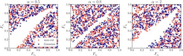
Figure 1: The points/crosses show the $F_{\nu_{e}}-F_{\bar{\nu}_{e}}$’s for which there is a crossing in the $\nu$ELN angular distribution for the maximum entropy and Gaussian distributions, for some values of $\alpha$. Note that the crossing (no-crossing) region patterns are very similar for the two angular distributions. The classifications can be different only at some narrow zones at the boundary of the crossing/no-crossing regions, where the labels get noisy meaning that there are different labels at the same point.

II.1 Parametric angular distributions

ML requires data to be trained, evaluated, and then tested on. In order to train and test our ML algorithms, we need a sufficient amount of labeled data containing $I_{0}$ and $I_{1}$ of $\nu_{e}$ and $\bar{\nu}_{e}$, where the labels determine whether $\nu$ELN crossing exists or not. Note that we here only focus on the first two moments since they are the ones which are normally directly followed in the simulations.

Though one can, in principle, use the very few available simulations where the neutrino angular distributions are directly available, we here train/test our ML algorithms by using parametric neutrino angular distributions. This choice is quite justifiable considering a number of observations. First, one should note that the moment-based CCSN and NSM simulations use different closure relations. This introduces some variations which depends on the type of the employed closure relation. Therefore, one should already expect a level of uncertainty in this problem once even the angular distributions from realistic simulations are used to train the ML algorithms. In addition and as indicated in Fig. 1, reasonable angular distributions should lead to similar patterns in the parameter space of $I_{0}$ and $I_{1}$, regarding the occurrence of $\nu$ELN crossings. This implies that the parametric angular distributions should be able to provide a reliable/acceptable evaluation of the occurrence of $\nu$ELN crossings, given the uncertainties already existing in CCSN and NSM simulations. We elaborate more on this later in this section when we test our ML algorithms for detecting $\nu$ELN crossings in a time snapshot of a NSM remnant simulation. Besides, considering parametric angular distributions helps one have access to a larger training dataset, hence reducing the risk of overfitting which could be crucial in this problem. Indeed, using parametric angular distributions provides one with a more generic training dataset, which as we see later on is very important in this problem.

We use two parametric neutrino angular distributions which have beed widely used in the literature. The first one is the maximum entropy distribution defined as,

$$f^{\rm{max-ent}}_{\nu}(\mu)=\exp[\eta+a\mu],$$ (3)

where we here consider the $\phi_{\nu}$-integrated distribution, i.e.,

$$f_{\nu}(\mu)=\int_{0}^{\infty}\int_{0}^{2\pi}\frac{E_{\nu}^{2}\mathrm{d}E_{\nu}\mathrm{d}\phi_{\nu}}{(2\pi)^{3}}f_{\nu}(\mathbf{p}).$$ (4)

This is a very natural choice for the neutrino angular distribution since the maximum entropy closure Cernohorsky:1994yg is currently very popular in the moment-based neutrino transport methods. This parametric distribution has been also used to detect $\nu$ELN crossings Richers:2022dqa . Another angular distribution considered in the literature of FFCs (see, e.g., Refs. Wu:2021uvt ; Yi:2019hrp ) is the Gaussian distribution defined as,

$$f^{\rm{Gauss}}_{\nu}(\mu)=A\exp[-\frac{(1-\mu)^{2}}{a}].$$ (5)

Note that both of these distributions have a parameter which determines the overall neutrino number density, namely $\eta$ and $A$, and the other parameter determining the shape of the distribution, i.e., $a$.

II.2 Feature engineering

Thought we here considered $I_{0}$ and $I_{1}$ of $\nu_{e}$ and $\bar{\nu}_{e}$ as the relevant information on its basis one should decide whether $\nu$ELN crossings exist or not, one should still find the best features on their basis $\nu$ELN crossings can be detected most efficiently. Given this, one should first keep in mind that an overall normalisation factor does not affect the occurrence of $\nu$ELN crossings. This lead us to consider only $I^{\bar{\nu}_{e}}_{0}/I^{\nu_{e}}_{0}$, instead of $I^{\bar{\nu}_{e}}_{0}$ and $I^{\nu_{e}}_{0}$ independently. In addition, one can do a similar sort of normalisation for $I^{\bar{\nu}_{e}}_{1}$ and $I^{\nu_{e}}_{1}$ given the fact that only the shapes of the angular distributions matter. Having said that, we consider

$$\alpha=I^{\bar{\nu}_{e}}_{0}/I^{\nu_{e}}_{0},\ F_{\nu_{e}}=I^{\nu_{e}}_{1}/I^{\nu_{e}}_{0},\ \mathrm{and}\ F_{\bar{\nu}_{e}}=I^{\bar{\nu}_{e}}_{1}/I^{\bar{\nu}_{e}}_{0},$$ (6)

as the relevant features to be considered in the ML algorithms in this problem.

II.3 Data preparation

To cover the $\alpha$ space more efficiently, we consider 84 bins in the range $\alpha=(0.03-2.5)$. Then for each $\alpha$, we generate 700 random points in the $F_{\nu_{e}}-F_{\bar{\nu}_{e}}$ parameter space for which we find the maximum entropy and Gaussian angular distributions and then determine whether a $\nu$ELN crossing exists or not.

In Fig. 1, we show the zones for which there is a crossing in the $\nu$ELN angular distribution, in the $F_{\nu_{e}}-F_{\bar{\nu}_{e}}$ parameter space for some values of $\alpha$. One should note that the crossing/no-crossing regions are very similar for the two angular distributions, apart from a narrow zone in the boundary between the crossing/no-crossing regions. The fact that there exists a sort of common pattern confirms that this problem can be addressed in the framework of ML and also again justifies the application of parametric angular distributions for training our ML algorithms.

In order to train/test the ML algorithms, one should split this dataset into three independent sets: i) The training set, which is used to train the ML algorithm, ii) The development set, which is used to find out the hyper-parameters of the algorithm, and iii) the test set, which provides a measure of the performance of the ML method on new unseen data.

II.4 Performance metrics

Before moving on to our ML algorithms, we would like to comment on different metrics used to evaluate the performance of a ML algorithm. Apart from accuracy which is perhaps the most trivial metric, one can also consider precision, recall, and $F_{1}$ metrics,

$$\begin{split}&\mathrm{accuracy}=\frac{T_{p}+T_{n}}{T_{p}+T_{n}+F_{p}+F_{n}}\\ &\mathrm{precision}=\frac{T_{p}}{T_{p}+F_{p}}\\ &\mathrm{recall}=\frac{T_{p}}{T_{p}+F_{n}}\\ &F_{1}=2\times\frac{\mathrm{precision}\times\mathrm{recall}}{\mathrm{precision}+\mathrm{recall}},\end{split}$$ (7)

with $T(F)_{p(n)}$ denoting True (False) positive (negative) classifications. An astute reader can see that the precision/recall metric provides information on the reliability/detectability of the positive classification, while $F_{1}$ is their harmonic mean. In this study, we consider the accuracy as the appropriate metric because we would like to be equally sensitive to the existence/absence of the ELN crossings.

II.5 ML algorithms

In this part, we discuss our results on detecting $\nu$ELN crossings with the application of ML algorithms. We first focus on Logistic Regression (LR), which turns out to be the most promising ML algorithm to be used in detecting $\nu$ELN crossings. Then for illustration purposes, we also discuss our results for a few other algorithms. The accuracies of different algorithms are presented in Table 1. Most of the methodologies of this part are available on GitHub.

LR is a classifier which uses the logistic function,

$$\sigma(s)={\frac{1}{1+e^{-s}}},$$ (8)

on top of a linear one, i.e., $s=\mathbf{x}^{T}\mathbf{w}$, where $\mathbf{x}$ and $\mathbf{w}$ are the features and the trained wights, respectively. If $\sigma(s)\geq p_{\mathrm{c}}$ (with $p_{\mathrm{c}}$ being a threshold probability which is here taken to be $p_{\mathrm{c}}=0.5$), then the point is classified into class 1 (crossing) and otherwise, into class 0 (no-crossing).

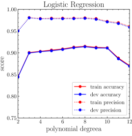
Figure 2: The accuracy and precision of the LR algorithm for the training and development datasets as a function of the polynomial degree of the nonlinear transformations. The scores reach their maximum at $n\simeq 9$, though they are more or less acceptable for $n\gtrsim 3$.

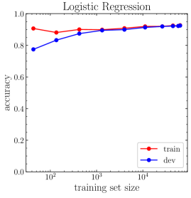
Figure 3: The accuracy of the LR algorithm for the training and development sets. Note that the overfitting disappears once at least a few thousand points are considered to train the LR algorithm.

Though LR includes the nonlinear logistic function, it is a linear classifier meaning that it can not be used directly to our problem, which obviously possesses non-linear patterns as presented in Fig. 1. To address this issue, one should first make non-linear transformations and generate new features out of the original three features in the problem. Python sklearn provides a module which does this, given the polynomial degree of the nonlinear transformation, which is a hyper-parameter of this algorithm.

In Fig. 2, we show the accuracy and precision of the LR algorithm for the training and development datasets. One can easily see that the accuracies reach their maximum at $n\simeq 8-10$, where $n$ is the polynomial degree, though we observed that $n=9$ performs a bit better once realistic data are considered (see Sec.II.6). Despite this, the metric scores are generally acceptable for $n\geq 3$.

A very interesting characteristic of the LR algorithm is in that it provides a probability interpretation of the classification. This is possible owing to the fact that the logistic function has a range of $(0,1)$. One can then write:

$$\begin{split}P(y=1|\mathbf{x},\mathbf{w})&=\sigma(\mathbf{x}^{T}\mathbf{w}),\\ P(y=0|\mathbf{x},\mathbf{w})&=1-P(y=1|\mathbf{x},\mathbf{w}).\end{split}$$ (9)

Such an interpretation is indeed very important in our application of ML in detecting $\nu$ELN crossings. This is because one can then play with the threshold probability, $p_{\mathrm{c}}$, to artificially facilitate/hinder the occurrence of FFCs in the regions of interest. This obviously provides one with a strong tool to measure the extent of the impact of FFCs on the CCSN and NSM physics.

Regarding the application of ML in detecting $\nu$ELN crossings in CCSN and NSM simulations, there is another important feature associated with the LR algorithm, namely its easy implementation. Indeed once the LR algorithm has been trained and $\mathbf{w}$’s have been learned, the LR algorithm can be directly implemented in CCSN and NSM simulation codes in a quite straightforward manner.

One of the most serious issues in ML is the overfitting problem, where the performance of the algorithm in the training set is significantly better than that of the test set, due to the unavailability of sufficient amount of data. This can lead to a remarkable variation in the performance once moving from one dataset to the other. In Fig. 3, we show the accuracy of LR as a function of the training set size. One can see that at least a few thousand data points should be available to avoid overfitting in this problem. Note that the size of the dataset is here determined by the number of $\alpha$’s multiplied by the number random points in the $F_{\nu_{e}}-F_{\bar{\nu}_{e}}$ parameter space. As we discuss later on, this number can be very sensitive to the range of $\alpha$ accessible in the training dataset. Therefore if some realistic angular distributions are used for training purposes, one should make sure that an appropriate range of $\alpha$ exists in the dataset.

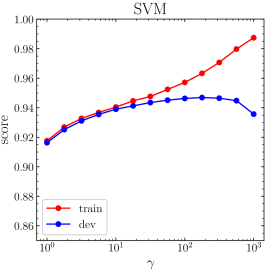
Figure 4: The accuracy of the SVM algorithm on the training and development sets, as a function of the $\gamma$ parameter defined in Eq. (10). The best performance of the SVM algorithm on the development set is reached at $\gamma\simeq 100$.

The next algorithm that we consider is the k-nearest neighbours (KNN) algorithm, in which the classification is made on the basis of the observation in the k-nearest neighbours. We here chose $k=3$, though we have confirmed that the performance does not change once other reasonable values for $k$ are considered. We also base our decision on the distance from the point. KNN is particularly appropriate for problems where the data points can suitably cover the whole parameter space and the observations closest to a given point should provide us with the most probable observation at that point. Though KNN is perhaps the simplest and most straightforward ML algorithm in many different respects, its implementation in detecting $\nu$ELN crossings in CCSN and NSM simulations may not be that efficient. This is because at any classification, one needs to load and analyze the whole training dataset, which could be computationally expensive.

Apart from LR and KNN, we also tried the performance of support vector machines (SVMs) with the radial basis function (RBF) kernel and decision tree (DT) algorithm. SVM tries to find the best hyperplane in the feature space, which separates the different classes in the dataset such that the margins are maximised. This means that the distance between the data points in different classes and the classifier hyperplane is maximum. The RBF kernel is defined as,

$$\mathcal{K}(x,x^{\prime})=\exp(-\gamma||x-x^{\prime}||^{2}),$$ (10)

where $\gamma$ is a hyper-parameter which needs to be determined by the evaluation of the SVM performance in the development set. The RBF kernel is based on finding similarities between the test data point and the ones in the training set, where $\gamma$ determines the distance up to which the similarities can efficiently make an impact.

As one can see in Fig. 4, the best performance of the SVM algorithm on the development set is obtained at $\gamma\simeq 100$. One should also note that the training set can reach an accuracy of $\sim 100\%$. This should come as no surprise since for very large $\gamma$’s, the decision for each point in the training set is mostly based on the observation at itself.

DT is another powerful method in classification and prediction, which has a flowchart-like tree structure. It include internal nodes and branches, where each internal node denotes a test on a feature and each branch represents the outcome of the test. There are also leaf nodes which can be considered as terminal nodes holding the class labels.

Table 1: A summary of the metric scores of our ML algorithms. Note that almost all the tried ML algorithms can easily reach scores more than $90\%$. In front of each algorithm, one can find its accuracy, i.e., LR, KNN, SVM, and DT have accuracies of 93%, 95%, 95%, and 94%, respectively. Though the LR algorithm scores can be less than the others by a few percents, its easy implementation and probabilistic interpretation makes it the most promising candidate ML algorithm to be used in detecting $\nu$ELN crossings.

	Logistic Regression (93%)
	precision	recall	$F_{1}$-score
no crossing	83%	93%	88%
crossing	97%	93%	95%
	KNN (n=3) (95%)
	precision	recall	$F_{1}$-score
no crossing	90%	90%	90%
crossing	96%	96%	96%
	SVM (95%)
	precision	recall	$F_{1}$-score
no crossing	92%	90%	91%
crossing	96%	97%	97%
	Decision tree (94%)
	precision	recall	$F_{1}$-score
no crossing	89%	88%	89%
crossing	96%	96%	96%

The general performances of our ML algorithms are presented in Table 1. As can be seen, all the ML algorithms can easily reach accuracies $\gtrsim 90\%$. One interesting point in Table 1 is that the precision/recall scores of the no-crossing class is systematically lower for all the ML algorithms. This can be explained given the fact that for our dataset, the regions of no-crossing are too close to the boundary region between crossings/no-crossing regions, which makes the classification more prone to error. This is well illustrated in the middle panel of Fig. 1, where the region of the no-crossing class is narrow and therefore many of the data points are too close to the boundary of the crossing/no-crossing regions, unlike what one has for the crossing class. However, one should bear in mind that this might be also just an artefact of the unrealistic dataset we utilise here and hence should be explored in more details once more realistic data are available. One should also note that the maximum accuracy is almost similar in all different algorithms, namely $\sim 95\%$. This is indeed the Bayes error rate of this problem, which is the maximum accuracy accessible in ideal situations. This implies that the ML algorithms do a fantastic job in our classification problem. As a matter of fact, the main source of error in this problem is the noisiness of the target labels. In other words, there are regions in the $F_{\nu_{e}}-F_{\bar{\nu}_{e}}$ parameter space for which the different parametric angular distributions lead to different results/labels regarding the existence of $\nu$ELN crossings. In this problem, one can find the maximum Bayes error rate by checking the asymptotic accuracy of the knn method once the number of data points goes to infinity. We have confirmed that the value of the Bayes error rate obtained this way is consistent with the values observed in Table 1, i.e., $\sim 95\%$.

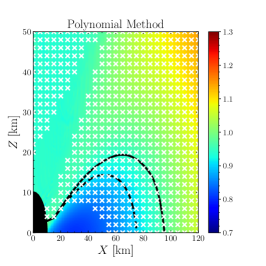
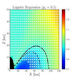
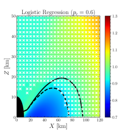
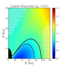
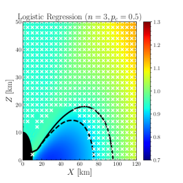
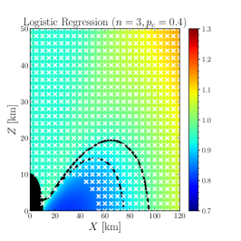
Figure 5: $\nu$ELN crossings (white crosses) in the polar plane of the axisymmetric simulation (model M3A8m3a5 from Ref. Just:2014fka ) at $t=50$ ms. The z axis is the symmetry axis and x is the cylindrical radius, the color map shows the $\nu_{e}-\bar{\nu}_{e}$ asymmetry parameter, $\alpha=n_{\bar{\nu}_{e}}/n_{\nu_{e}}$, and the solid (dashed) lines indicate the locations of the $\nu_{e}$ ($\bar{\nu}_{e}$) neutrinospheres. While the upper left panel shows the crossings captured by the polynomial method, the rest of the panels indicate the $\nu$ELN crossings captured by the LR algorithm with different threshold densities, $p_{c}$, and polynomial degrees ($n=9$ for the upper right and lower left panels and $n=3$ for the lower middle and right panels).

II.6 Applying ML to a NSM remnant simulation

Having trained and tested our ML algorithms by the parametric neutrino angular distributions, we now test them also on some realistic data obtained from simulations of a NSM remnant (model M3A8m3a5 from Ref. Just:2014fka ). This way, one can get a flavor of how our ML algorithms perform on datasets which are remarkably different from what they have been trained on. This data has been explored in Ref. Just2022c , where the polynomial method developed in Ref. Abbar:2020fcl was used to detect $\nu$ELN crossings. As discussed before, the advantage of the polynomial method is in that it is very accurate in what it can detect, i.e., it has a precision of $100\%$, though its recall is not guaranteed to be high.

In Fig. 5, we present our results on using different methods to detect $\nu$ELN crossings in the simulation of the NSM remnant model studied in Ref. Just2022c , in the time snapshot $t=50$ ms. The upper left panel shows the crossings captured by the polynomial method, which is similar to Fig. 1 of the Ref. Just2022c . The rest of the panels indicate the $\nu$ELN crossings captured by the LR algorithm with different threshold densities, $p_{c}$, and polynomial degrees. As one can clearly see, all the $\nu$ELN crossings captured by the polynomial method can be also detected by the LR algorithm with $p_{c}=0.5$ (upper middle panel). Besides, LR can detect a number of other $\nu$ELN crossings, particularly in the region where $\alpha\simeq 1$. This is, in fact, not surprising. As also discussed in Ref. Just2022c , the $\nu$ELN crossings are very likely to occur in this regions. However, the polynomial method can miss these crossings due to its important limitations regarding its dependence on the amount of available neutrino angular information, i.e., the number of available moments. But the ML method does not have this limitation and it is not surprising that it captures a number of crossings in this region. There is indeed an important observation here. Once machine learning is considered, the information of the angular distribution shape leaks from the data to the decision maker. So although the higher moments are not available, one has still some information about them coming from the patterns in the data. In contrast, in the polynomial method the information is solely provided through the angular moments. In addition, the number of detected crossings decreases with increasing $p_{c}$, as expected (upper right and lower left panels). In all these three panels, the polynomial degree is taken to be $n=9$.

Though the best accuracy of the LR algorithm is reached for $n=9$, the accuracy is more or less acceptable for $n\geq 3$. Specifically, $n=3$ is an interesting case given the fact that it requires much less amount of computations. In the lower middle and right panels of Fig. 5, the LR classification results with $n=3$ are presented for $p_{c}=0.5$ and $0.4$, respectively. Though the accuracy of the LR algorithm with $n=3$ is lower than that of $n=9$, it can capture almost all the $\nu$ELN crossings detected by the LR algorithm for $n=9$ and $p_{c}=0.5$, once lower $p_{c}$ is tried (lower right panel).

We noticed that the accuracy of the ML algorithms could be remarkably reduced if the $\alpha$ range of the test set is significantly outside the one of the training set. This implies that to have an accurate ML algorithm, one should have access to a very generic training set including all the relevant values of $\alpha$. This can be indeed difficult given the scarceness of realistic neutrino angular distributions. This again justifies the application of the parametric angular distributions to training the ML algorithms.

We have here only discussed the results of the LR algorithm due to its importance in detecting $\nu$ELN crossings. But the other algorithms also perform similarly well on this model. Though our ML algorithms were trained on some parametric angular distributions, they performed remarkably well on some realistic data they had never seen. We consider this as a very promising sign of the applicability of ML in detecting $\nu$ELN crossings in the most extreme astrophysical settings (models).

III DISCUSSION AND OUTLOOK

We have studied the application of ML to detecting $\nu$ELN crossings in CCSN and NSM models. Unlike the other existing methods which are either inefficient or very slow, once trained, ML can be very fast and efficient in detecting the $\nu$ELN crossings. Hence, it provides one with a strong tool to explore FFCs in CCSN and NSM simulations on the fly. We show that ML algorithms can reach very high accuracies, $\sim 95\%$, which is almost the Bayes error rate of this problem, though the exact accuracy should depend on the environment where the ML algorithms are employed.

For training our ML algorithms, we used two parametric neutrino angular distributions already considered in the literature, namely the maximum entropy and the Gaussian distributions. Choosing such parametric distributions helps overcome the overfitting, which can be particularly serious in this problem. To be more specific, ML classifications can be very sensitive to the accessible values of $\alpha$ in the training set.

Of particular interest is the LR algorithm which can be easily implemented in CCSN and NSM simulations. At the same time, the probabilistic interpretation of LR allows one to have a strong tool to control/evaluate the the extent of the impact of FFCs on the physics of CCSNe and NSMs.

In order to check the efficiency and reliability of our trained ML algorithms, we tested them on some data obtained from a realistic NSM remnant simulation. Though the ML algorithms had never seen such data, they perform remarkably well on them. We consider this as a very promising achievement supporting the application of ML to detecting $\nu$ELN crossings in NSM and CCSN simulations. Despite this, we would like to emphasise that our study is just meant to introduce this novel idea and more research is still required to train more accurate ML algorithms to detecting $\nu$ELN crossings in realistic NSM and CCSN models.

One of the limitations of our study is that our ML algorithms are only sensitive to the crossings in the $\nu$ELN angular distribution once it is integrated over $\phi$. In realistic CCSN and NSM simulations, there could exist $\nu$ELN crossings in the $\phi$ direction, if the the angular distribution is asymmetric enough in $\phi$. For such cases, one should use directly the realistic data since reasonable parametric angular distributions do not currently exist. If such data are available, one should also consider a larger number of features in the ML method since the $\phi$-related moments can also play a role. Another limitation of our research comes from the assumption that the angular distributions of $\nu_{x}$ and $\bar{\nu}_{x}$ are the same. In realistic situations, one can have $f_{\nu_{x}}\neq f_{\bar{\nu}_{x}}$, particularly due to the creation of muons in the densest regions of CCSN and NSM environments Bollig:2017lki ; Capozzi:2020syn . This makes it necessary to explore ML algorithms which are capable of detecting $\nu$ELN crossings once $\nu_{x}$ and $\bar{\nu}_{x}$ are taken into account separately.

In brief, though our study provides the first step in applying ML techniques to exploring FFCs in CCSN and NSM simulations and proves their applicability in this business, further research is still required to investigate more realistic and complicated situations.

References

- (1) J. T. Pantaleone, Neutrino oscillations at high densities, Phys. Lett. B287 (1992) 128–132. doi:10.1016/0370-2693(92)91887-F.
- (2) G. Sigl, G. Raffelt, General kinetic description of relativistic mixed neutrinos, Nuclear Physics B 406 (1-2) (1993) 423–451.
- (3) S. Pastor, G. Raffelt, Flavor oscillations in the supernova hot bubble region: Nonlinear effects of neutrino background, Phys. Rev. Lett. 89 (2002) 191101. arXiv:astro-ph/0207281, doi:10.1103/PhysRevLett.89.191101.
- (4) H. Duan, G. M. Fuller, J. Carlson, Y.-Z. Qian, Simulation of Coherent Non-Linear Neutrino Flavor Transformation in the Supernova Environment. 1. Correlated Neutrino Trajectories, Phys. Rev. D 74 (2006) 105014. arXiv:astro-ph/0606616, doi:10.1103/PhysRevD.74.105014.
- (5) H. Duan, G. M. Fuller, J. Carlson, Y.-Z. Qian, Coherent Development of Neutrino Flavor in the Supernova Environment, Phys. Rev. Lett. 97 (2006) 241101. arXiv:astro-ph/0608050, doi:10.1103/PhysRevLett.97.241101.
- (6) H. Duan, G. M. Fuller, Y.-Z. Qian, Collective Neutrino Oscillations, Ann. Rev. Nucl. Part. Sci. 60 (2010) 569–594. arXiv:1001.2799, doi:10.1146/annurev.nucl.012809.104524.
- (7) A. Mirizzi, I. Tamborra, H.-T. Janka, N. Saviano, K. Scholberg, R. Bollig, L. Hüdepohl, S. Chakraborty, Supernova neutrinos: Production, oscillations and detection, Riv. Nuovo Cim. 39 (1-2) (2016) 1–112. arXiv:1508.00785, doi:10.1393/ncr/i2016-10120-8.
- (8) M. C. Volpe, Neutrinos from dense: flavor mechanisms, theoretical approaches, observations, new directions (1 2023). arXiv:2301.11814.
- (9) R. F. Sawyer, Speed-up of neutrino transformations in a supernova environment, Phys. Rev. D 72 (2005) 045003. arXiv:hep-ph/0503013, doi:10.1103/PhysRevD.72.045003.
- (10) R. F. Sawyer, Neutrino cloud instabilities just above the neutrino sphere of a supernova, Phys. Rev. Lett. 116 (8) (2016) 081101. arXiv:1509.03323, doi:10.1103/PhysRevLett.116.081101.
- (11) S. Chakraborty, R. S. Hansen, I. Izaguirre, G. Raffelt, Self-induced neutrino flavor conversion without flavor mixing, JCAP 03 (2016) 042. arXiv:1602.00698, doi:10.1088/1475-7516/2016/03/042.
- (12) I. Izaguirre, G. Raffelt, I. Tamborra, Fast Pairwise Conversion of Supernova Neutrinos: A Dispersion-Relation Approach, Phys. Rev. Lett. 118 (2) (2017) 021101. arXiv:1610.01612, doi:10.1103/PhysRevLett.118.021101.
- (13) F. Capozzi, B. Dasgupta, E. Lisi, A. Marrone, A. Mirizzi, Fast flavor conversions of supernova neutrinos: Classifying instabilities via dispersion relations, Phys. Rev. D 96 (4) (2017) 043016. arXiv:1706.03360, doi:10.1103/PhysRevD.96.043016.
- (14) S. Abbar, M. C. Volpe, On Fast Neutrino Flavor Conversion Modes in the Nonlinear Regime, Phys. Lett. B 790 (2019) 545–550. arXiv:1811.04215, doi:10.1016/j.physletb.2019.02.002.
- (15) F. Capozzi, B. Dasgupta, A. Mirizzi, M. Sen, G. Sigl, Collisional triggering of fast flavor conversions of supernova neutrinos, Phys. Rev. Lett. 122 (9) (2019) 091101. arXiv:1808.06618, doi:10.1103/PhysRevLett.122.091101.
- (16) J. D. Martin, C. Yi, H. Duan, Dynamic fast flavor oscillation waves in dense neutrino gases, Phys. Lett. B 800 (2020) 135088. arXiv:1909.05225, doi:10.1016/j.physletb.2019.135088.
- (17) F. Capozzi, G. Raffelt, T. Stirner, Fast Neutrino Flavor Conversion: Collective Motion vs. Decoherence, JCAP 09 (2019) 002. arXiv:1906.08794, doi:10.1088/1475-7516/2019/09/002.
- (18) L. Johns, H. Nagakura, G. M. Fuller, A. Burrows, Neutrino oscillations in supernovae: angular moments and fast instabilities, Phys. Rev. D 101 (4) (2020) 043009. arXiv:1910.05682, doi:10.1103/PhysRevD.101.043009.
- (19) J. D. Martin, J. Carlson, V. Cirigliano, H. Duan, Fast flavor oscillations in dense neutrino media with collisions, Phys. Rev. D 103 (2021) 063001. arXiv:2101.01278, doi:10.1103/PhysRevD.103.063001.
- (20) I. Tamborra, S. Shalgar, New Developments in Flavor Evolution of a Dense Neutrino Gas, Ann. Rev. Nucl. Part. Sci. 71 (2021) 165–188. arXiv:2011.01948, doi:10.1146/annurev-nucl-102920-050505.
- (21) G. Sigl, Simulations of fast neutrino flavor conversions with interactions in inhomogeneous media, Phys. Rev. D 105 (4) (2022) 043005. arXiv:2109.00091, doi:10.1103/PhysRevD.105.043005.
- (22) C. Kato, H. Nagakura, T. Morinaga, Neutrino Transport with the Monte Carlo Method. II. Quantum Kinetic Equations, Astrophys. J. Supp. 257 (2) (2021) 55. arXiv:2108.06356, doi:10.3847/1538-4365/ac2aa4.
- (23) T. Morinaga, Fast neutrino flavor instability and neutrino flavor lepton number crossings, Phys. Rev. D 105 (10) (2022) L101301. arXiv:2103.15267, doi:10.1103/PhysRevD.105.L101301.
- (24) H. Nagakura, L. Johns, A. Burrows, G. M. Fuller, Where, when, and why: Occurrence of fast-pairwise collective neutrino oscillation in three-dimensional core-collapse supernova models, Phys. Rev. D 104 (8) (2021) 083025. arXiv:2108.07281, doi:10.1103/PhysRevD.104.083025.
- (25) H. Sasaki, T. Takiwaki, A detailed analysis of the dynamics of fast neutrino flavor conversions with scattering effects, PTEP 2022 (7) (2022) 073E01. arXiv:2109.14011, doi:10.1093/ptep/ptac082.
- (26) I. Padilla-Gay, I. Tamborra, G. G. Raffelt, Neutrino Flavor Pendulum Reloaded: The Case of Fast Pairwise Conversion, Phys. Rev. Lett. 128 (12) (2022) 121102. arXiv:2109.14627, doi:10.1103/PhysRevLett.128.121102.
- (27) S. Abbar, F. Capozzi, R. Glas, H.-T. Janka, I. Tamborra, On the characteristics of fast neutrino flavor instabilities in three-dimensional core-collapse supernova models, Phys. Rev. D 103 (6) (2021) 063033. arXiv:2012.06594, doi:10.1103/PhysRevD.103.063033.
- (28) F. Capozzi, S. Abbar, R. Bollig, H. T. Janka, Fast neutrino flavor conversions in one-dimensional core-collapse supernova models with and without muon creation, Phys. Rev. D 103 (6) (2021) 063013. arXiv:2012.08525, doi:10.1103/PhysRevD.103.063013.
- (29) M. Delfan Azari, S. Yamada, T. Morinaga, W. Iwakami, H. Okawa, H. Nagakura, K. Sumiyoshi, Linear Analysis of Fast-Pairwise Collective Neutrino Oscillations in Core-Collapse Supernovae based on the Results of Boltzmann Simulations, Phys. Rev. D 99 (10) (2019) 103011. arXiv:1902.07467, doi:10.1103/PhysRevD.99.103011.
- (30) A. Harada, H. Nagakura, Prospects of Fast Flavor Neutrino Conversion in Rotating Core-collapse Supernovae, Astrophys. J. 924 (2) (2022) 109. arXiv:2110.08291, doi:10.3847/1538-4357/ac38a0.
- (31) I. Padilla-Gay, I. Tamborra, G. G. Raffelt, Neutrino fast flavor pendulum. II. Collisional damping, Phys. Rev. D 106 (10) (2022) 103031. arXiv:2209.11235, doi:10.1103/PhysRevD.106.103031.
- (32) F. Capozzi, M. Chakraborty, S. Chakraborty, M. Sen, Supernova fast flavor conversions in 1+1D: Influence of mu-tau neutrinos, Phys. Rev. D 106 (8) (2022) 083011. arXiv:2205.06272, doi:10.1103/PhysRevD.106.083011.
- (33) M. Zaizen, H. Nagakura, Simple method for determining asymptotic states of fast neutrino-flavor conversion (11 2022). arXiv:2211.09343.
- (34) S. Shalgar, I. Tamborra, Supernova Neutrino Decoupling Is Altered by Flavor Conversion (6 2022). arXiv:2206.00676.
- (35) C. Kato, H. Nagakura, Effects of energy-dependent scatterings on fast neutrino flavor conversions, Phys. Rev. D 106 (12) (2022) 123013. arXiv:2207.09496, doi:10.1103/PhysRevD.106.123013.
- (36) S. Bhattacharyya, B. Dasgupta, Fast Flavor Depolarization of Supernova Neutrinos, Phys. Rev. Lett. 126 (6) (2021) 061302. arXiv:2009.03337, doi:10.1103/PhysRevLett.126.061302.
- (37) M.-R. Wu, M. George, C.-Y. Lin, Z. Xiong, Collective fast neutrino flavor conversions in a 1D box: Initial conditions and long-term evolution, Phys. Rev. D 104 (10) (2021) 103003. arXiv:2108.09886, doi:10.1103/PhysRevD.104.103003.
- (38) S. Richers, D. E. Willcox, N. M. Ford, A. Myers, Particle-in-cell Simulation of the Neutrino Fast Flavor Instability, Phys. Rev. D 103 (8) (2021) 083013. arXiv:2101.02745, doi:10.1103/PhysRevD.103.083013.
- (39) S. Richers, D. Willcox, N. Ford, Neutrino fast flavor instability in three dimensions, Phys. Rev. D 104 (10) (2021) 103023. arXiv:2109.08631, doi:10.1103/PhysRevD.104.103023.
- (40) B. Dasgupta, Collective Neutrino Flavor Instability Requires a Crossing, Phys. Rev. Lett. 128 (8) (2022) 081102. arXiv:2110.00192, doi:10.1103/PhysRevLett.128.081102.
- (41) H. Nagakura, M. Zaizen, Time-Dependent and Quasisteady Features of Fast Neutrino-Flavor Conversion, Phys. Rev. Lett. 129 (26) (2022) 261101. arXiv:2206.04097, doi:10.1103/PhysRevLett.129.261101.
- (42) J. Ehring, S. Abbar, H.-T. Janka, G. Raffelt, Fast Neutrino Flavor Conversion in Core-Collapse Supernovae: A Parametric Study in 1D Models (1 2023). arXiv:2301.11938.
- (43) O. Just, M. Obergaulinger, H. Janka, A new multidimensional, energy-dependent two-moment transport code for neutrino-hydrodynamics, Mon. Not. Roy. Astron. Soc. 453 (4) (2015) 3386–3413. arXiv:1501.02999, doi:10.1093/mnras/stv1892.
- (44) L. M. Murchikova, E. Abdikamalov, T. Urbatsch, Analytic Closures for M1 Neutrino Transport, Mon. Not. Roy. Astron. Soc. 469 (2) (2017) 1725–1737. arXiv:1701.07027, doi:10.1093/mnras/stx986.
- (45) B. Dasgupta, A. Mirizzi, M. Sen, Simple method of diagnosing fast flavor conversions of supernova neutrinos, Phys. Rev. D98 (10) (2018) 103001. arXiv:1807.03322, doi:10.1103/PhysRevD.98.103001.
- (46) L. Johns, H. Nagakura, Fast flavor instabilities and the search for neutrino angular crossings, Phys. Rev. D 103 (12) (2021) 123012. arXiv:2104.04106, doi:10.1103/PhysRevD.103.123012.
- (47) S. Abbar, Searching for Fast Neutrino Flavor Conversion Modes in Core-collapse Supernova Simulations, JCAP 05 (2020) 027. arXiv:2003.00969, doi:10.1088/1475-7516/2020/05/027.
- (48) S. Richers, Evaluating approximate flavor instability metrics in neutron star mergers, Phys. Rev. D 106 (8) (2022) 083005. arXiv:2206.08444, doi:10.1103/PhysRevD.106.083005.
- (49) D. George, E. A. Huerta, Deep Learning for Real-time Gravitational Wave Detection and Parameter Estimation: Results with Advanced LIGO Data, Phys. Lett. B 778 (2018) 64–70. arXiv:1711.03121, doi:10.1016/j.physletb.2017.12.053.
- (50) R. Qiu, P. Krastev, K. Gill, E. Berger, Deep Learning Detection and Classification of Gravitational Waves from Neutron Star-Black Hole Mergers (10 2022). arXiv:2210.15888.
- (51) J. a. Aveiro, F. F. Freitas, M. Ferreira, A. Onofre, C. Providência, G. Gonçalves, J. A. Font, Identification of binary neutron star mergers in gravitational-wave data using object-detection machine learning models, Phys. Rev. D 106 (8) (2022) 084059. arXiv:2207.00591, doi:10.1103/PhysRevD.106.084059.
- (52) P. G. Krastev, Real-Time Detection of Gravitational Waves from Binary Neutron Stars using Artificial Neural Networks, Phys. Lett. B 803 (2020) 135330. arXiv:1908.03151, doi:10.1016/j.physletb.2020.135330.
- (53) W. Wei, E. A. Huerta, Deep learning for gravitational wave forecasting of neutron star mergers, Phys. Lett. B 816 (2021) 136185. arXiv:2010.09751, doi:10.1016/j.physletb.2021.136185.
- (54) M. B. Schäfer, F. Ohme, A. H. Nitz, Detection of gravitational-wave signals from binary neutron star mergers using machine learning, Phys. Rev. D 102 (6) (2020) 063015. arXiv:2006.01509, doi:10.1103/PhysRevD.102.063015.
- (55) A. Mitra, B. Shukirgaliyev, Y. S. Abylkairov, E. Abdikamalov, Exploring Supernova Gravitational Waves with Machine Learning (9 2022). arXiv:2209.14542, doi:10.1093/mnras/stad169.
- (56) M. López Portilla, I. D. Palma, M. Drago, P. Cerdá-Durán, F. Ricci, Deep learning for core-collapse supernova detection, Phys. Rev. D 103 (6) (2021) 063011. arXiv:2011.13733, doi:10.1103/PhysRevD.103.063011.
- (57) B. T. H. Tsang, D. Vartanyan, A. Burrows, Applications of Machine Learning to Predicting Core-collapse Supernova Explosion Outcomes, Astrophys. J. Lett. 937 (1) (2022) L15. arXiv:2208.01661, doi:10.3847/2041-8213/ac8f4b.
- (58) P. I. Karpov, C. Huang, I. Sitdikov, C. L. Fryer, S. Woosley, G. Pilania, Physics-informed Machine Learning for Modeling Turbulence in Supernovae, Astrophys. J. 940 (1) (2022) 26. arXiv:2205.08663, doi:10.3847/1538-4357/ac88cc.
- (59) P. Mehta, M. Bukov, C.-H. Wang, A. G. R. Day, C. Richardson, C. K. Fisher, D. J. Schwab, A high-bias, low-variance introduction to Machine Learning for physicists, Phys. Rept. 810 (2019) 1–124. arXiv:1803.08823, doi:10.1016/j.physrep.2019.03.001.
- (60) J. Cernohorsky, S. A. Bludman, Maximum entropy distribution and closure for Bose-Einstein and Fermi-Dirac radiation transport (3 1994).
- (61) C. Yi, L. Ma, J. D. Martin, H. Duan, Dispersion relation of the fast neutrino oscillation wave, Phys. Rev. D 99 (6) (2019) 063005. arXiv:1901.01546, doi:10.1103/PhysRevD.99.063005.
- (62) O. Just, A. Bauswein, R. A. Pulpillo, S. Goriely, H. T. Janka, Comprehensive nucleosynthesis analysis for ejecta of compact binary mergers, Mon. Not. Roy. Astron. Soc. 448 (1) (2015) 541–567. arXiv:1406.2687, doi:10.1093/mnras/stv009.
- (63) O. Just, S. Abbar, M.-R. Wu, I. Tamborra, H.-T. Janka, F. Capozzi, Fast neutrino conversion in hydrodynamic simulations of neutrino-cooled accretion disks, Phys. Rev. D105 (8) (2022) 083024. arXiv:2203.16559, doi:10.1103/PhysRevD.105.083024.
- (64) R. Bollig, H. T. Janka, A. Lohs, G. Martinez-Pinedo, C. J. Horowitz, T. Melson, Muon Creation in Supernova Matter Facilitates Neutrino-driven Explosions, Phys. Rev. Lett. 119 (24) (2017) 242702. arXiv:1706.04630, doi:10.1103/PhysRevLett.119.242702.
- (65) F. Pedregosa, G. Varoquaux, A. Gramfort, V. Michel, B. Thirion, O. Grisel, M. Blondel, P. Prettenhofer, R. Weiss, V. Dubourg, et al., Scikit-learn: Machine learning in python, Journal of machine learning research 12 (Oct) (2011) 2825–2830.
- (66) J. D. Hunter, Matplotlib: A 2D Graphics Environment, Computing in Science & Engineering 9 (3) (2007) 90–95. doi:10.1109/MCSE.2007.55.
-
(67)
C. R. Harris, K. J. Millman, S. J. van der Walt, R. Gommers, P. Virtanen,
D. Cournapeau, E. Wieser, J. Taylor, S. Berg, N. J. Smith, R. Kern, M. Picus,
S. Hoyer, M. H. van Kerkwijk, M. Brett, A. Haldane, J. F. del Río,
M. Wiebe, P. Peterson, P. Gérard-Marchant, K. Sheppard, T. Reddy,
W. Weckesser, H. Abbasi, C. Gohlke, T. E. Oliphant,
Array programming with
NumPy, Nature 585 (7825) (2020) 357–362.
doi:10.1038/s41586-020-2649-2.
URL https://doi.org/10.1038/s41586-020-2649-2 - (68) P. Virtanen, R. Gommers, T. E. Oliphant, M. Haberland, T. Reddy, D. Cournapeau, E. Burovski, P. Peterson, W. Weckesser, J. Bright, S. J. van der Walt, M. Brett, J. Wilson, K. J. Millman, N. Mayorov, A. R. J. Nelson, E. Jones, R. Kern, E. Larson, C. J. Carey, İ. Polat, Y. Feng, E. W. Moore, J. VanderPlas, D. Laxalde, J. Perktold, R. Cimrman, I. Henriksen, E. A. Quintero, C. R. Harris, A. M. Archibald, A. H. Ribeiro, F. Pedregosa, P. van Mulbregt, SciPy 1.0 Contributors, SciPy 1.0: Fundamental Algorithms for Scientific Computing in Python, Nature Methods 17 (2020) 261–272. doi:10.1038/s41592-019-0686-2.
-
(69)
F. Pérez, B. E. Granger, IPython: a system for
interactive scientific computing, Computing in Science and Engineering 9 (3)
(2007) 21–29.
doi:10.1109/MCSE.2007.53.
URL https://ipython.org