Fast post-process Bayesian inference with
Sparse Variational Bayesian Monte Carlo

Abstract

We introduce Sparse Variational Bayesian Monte Carlo (svbmc), a method for fast “post-process” Bayesian inference for models with black-box and potentially noisy likelihoods. svbmc reuses all existing target density evaluations – for example, from previous optimizations or partial Markov Chain Monte Carlo runs – to build a sparse Gaussian process (GP) surrogate model of the log posterior density. Uncertain regions of the surrogate are then refined via active learning as needed. Our work builds on the Variational Bayesian Monte Carlo (vbmc) framework for sample-efficient inference, with several novel contributions. First, we make vbmc scalable to a large number of pre-existing evaluations via sparse GP regression, deriving novel Bayesian quadrature formulae and acquisition functions for active learning with sparse GPs. Second, we introduce noise shaping, a general technique to induce the sparse GP approximation to focus on high posterior density regions. Third, we prove theoretical results in support of the svbmc refinement procedure. We validate our method on a variety of challenging synthetic scenarios and real-world applications. We find that svbmc consistently builds good posterior approximations by post-processing of existing model evaluations from different sources, often requiring only a small number of additional density evaluations.

1 INTRODUCTION

Bayesian inference is a principled approach to uncertainty quantification and model selection, widely adopted in data science and machine learning [Robert et al., 2007, Gelman et al., 2013, Ghahramani, 2015]. Key quantities in Bayesian inference are the posterior distribution of model parameters, useful for parameter estimation, and the marginal likelihood or model evidence, useful for model selection. Practical implementation of Bayesian inference can be particularly challenging when dealing with models with ‘black-box’ features common in science and engineering, such as lack of gradients and mildly-to-very expensive and possibly noisy evaluations of the likelihood, e.g., arising from simulator-based estimation [Wood, 2010, van Opheusden et al., 2020].

Due to the cost of inference, the workflow of Bayesian analyses often starts with a preliminary exploration phase via simpler and cheaper means [Gelman et al., 2020]. A popular choice consists of performing maximum-a-posteriori (MAP) estimation, i.e., finding the (global) mode of the posterior, often via multiple runs of a black-box optimization algorithm [Acerbi and Ma, 2017]. In fact, due to prohibitive costs, many analyses stop here, with a point estimate instead of a full posterior. Another common approach consists of launching short runs of multiple Markov Chain Monte Carlo chains (mcmc; Robert et al. 2009). Short chains are unlikely to achieve statistical mixing and are subsequently discarded (with some exceptions, Yao et al. 2022). Discarding evaluations is a standard part of mcmc, throwing away as much as half of the samples used for tuning [Carpenter et al., 2017].

In this paper, we propose post-process Bayesian inference as a solution to the waste of potentially expensive posterior evaluations, with the goal of making ‘black-box’ Bayesian inference cheaper and more applicable. Namely, we aim to build an approximation of the full Bayesian posterior by recycling all previous evaluations of the posterior density (not just the outputs) coming from preliminary runs of other exploratory algorithms, whether optimization, mcmc, or others, and regardless of their convergence. Having put no restrictions on these initial samples, we allow our method to refine the solution at post-processing time with a minimal number of additional evaluations of the target posterior.

A natural framework compatible with our goals is that of Variational Bayesian Monte Carlo (vbmc; Acerbi 2018), originally proposed to tackle the challenge of black-box, sample-efficient Bayesian inference. vbmc approximates the target log-posterior with a surrogate statistical model, a Gaussian process (GP; Rasmussen and Williams 2005), iteratively improved via active learning [Jones et al., 1998, Snoek et al., 2012]. At the same time, vbmc computes a fast, tractable approximation of the posterior thanks to variational inference and Bayesian quadrature [O’Hagan, 1991, Ghahramani and Rasmussen, 2002b], which yields a lower bound to the model evidence. vbmc works with noisy likelihoods [Acerbi, 2020] and has been applied in fields such as neuroscience [Stine et al., 2020], nuclear engineering [Che et al., 2021], and cancer research [Demetriades et al., 2022].

An obstacle, however, comes from the fact that vbmc is built for – and only applies to – the ‘small evaluation’ setting (up to a few hundred posterior evaluations), due to known limitations of the GP model it is based on. For our goals, we need the method to scale to potentially tens of thousands evaluations coming from preliminary exploration of the posterior. Thus, in this paper we extend the vbmc framework by using scalable GP techniques – specifically, sparse GPs [Titsias, 2009, Hensman et al., 2013] – such that we can deal with a large initial set of evaluations of the target.

Outline and contributions.

We first recap the background methods, vbmc and sparse GPs, in Section 2. In Section 3, we describe how we combine the two in our novel framework, sparse Variational Bayesian Monte Carlo (svbmc). In the process, we derive novel sparse Bayesian quadrature formulae (Section 3.3) and acquisition functions for the sparse setting (Section 3.4), and propose a simple, principled heuristic (noise shaping; Section 3.5) to make the sparse GP representation focus on regions of interest. In Section 4, we present theoretical results in support of the consistency of our method. Section 5 validates svbmc on challenging synthetic and real-world examples. Finally, Section 6 reviews related work and Section 7 discusses strengths and limitations of our approach.

2 BACKGROUND

2.1 Variational Bayesian Monte Carlo

As described in the introduction, Variational Bayesian Monte Carlo (vbmc; Acerbi, 2018, 2019) is a sample-efficient Bayesian inference method that uses active learning to iteratively build a Gaussian process (GP) surrogate model of the target log posterior with a small number of likelihood evaluations. Approximate inference is then performed on the GP surrogate model in lieu of the more expensive target. In each iteration, a flexible mixture of Gaussians $q_{\phi}$ is fit to the surrogate model via variational inference. The optimization step is very efficient thanks to Bayesian quadrature [O’Hagan, 1991], which affords closed-form expressions for the variational objective providing a lower bound to the model evidence (elbo). Subsequent work [Acerbi, 2020] extended the framework with acquisition functions designed for noisy evaluations of the target [Järvenpää et al., 2019], often associated with simulator-based estimation of the log-likelihood [Wood, 2010, van Opheusden et al., 2020].

While other methods for sample-efficient Bayesian inference have been proposed (see Related Work in Section 6), vbmc has proven its efficiency and robustness in a variety of both noiseless and noisy scenarios, so it is a natural choice to build upon for developing a method for post-process, black-box Bayesian inference. A recap of vbmc and its foundations (variational inference, GPs, Bayesian quadrature) is given in Appendix A.

2.2 Sparse Variational Gaussian Process

Standard ‘exact’ GPs scale badly to a large number of training points $N$ (posterior evaluations in vbmc), typically $O(N^{3})$ due to the Gram’s matrix inversion. Sparse GPs have been proposed to reduce the computational burden of exact GPs [Snelson and Ghahramani, 2006, Titsias, 2009, Hensman et al., 2013]. Briefly, a sparse GP approximates the full GP with training inputs $\mathbf{X}=\{\mathbf{x}_{1},\ldots,\mathbf{x}_{N}\}$ by constructing a GP on a smaller set of inducing points $\mathbf{Z}=\{\mathbf{z}_{1},\ldots,\mathbf{z}_{M}\}$, with $M\ll N$. Sparse GP methods differ in the training objective that yields the distribution of inducing variables $\mathbf{u}$ (values of the sparse GP at the inducing points) used to approximate the full GP. Here we use sparse variational GP regression (sgpr; Titsias, 2009). In sgpr, for fixed sparse GP hyperparameters (e.g., length and output scales of the GP kernel) and inducing point locations, the posterior distribution of inducing variables is assumed to be multivariate normal whose mean vector $\mathbf{m}_{\mathbf{u}}$ and covariance matrix $\mathbf{S}_{\mathbf{u}\mathbf{u}}$ are conveniently available in closed form [Titsias, 2009].

Sparse GPs reduce the computational cost to $O(NM^{2})$. A major practical issue, though, is the placement of inducing points, especially in the sequential setting. While sgpr provides a principled way to select the inducing point locations, by treating them as variational parameters, a full optimization can be very expensive in practice, neutralizing the computational advantage of sparse GPs. Common approaches include selecting a subset of training points [Burt et al., 2020] or techniques for online adaptation of sparse GP hyperparameters and inducing point locations [Cheng and Boots, 2016, Galy-Fajou and Opper, 2021].

3 SPARSE VARIATIONAL BAYESIAN MONTE CARLO

In this section, we present our framework for post-process Bayesian inference, which we call Sparse Variational Bayesian Monte Carlo (svbmc). An implementation of the algorithm will be made available at https://github.com/pipme/svbmc.

Notation.

We denote with $f_{0}(\mathbf{x})\equiv\log p(\text{data}|\mathbf{x})p(\mathbf{x})$ the target (unnormalized) log posterior, where $p(\text{data}|\mathbf{x})$ is the likelihood of the model of interest under the data, $p(\mathbf{x})$ is the prior, and $\mathbf{x}\in\mathcal{X}\subseteq\mathbb{R}^{D}$ is a vector of model parameters. We indicate with $(\mathbf{x}_{n},y_{n})$ pairs of observed locations and values of the log-density, i.e., $y_{n}=f_{0}(\mathbf{x}_{n})$, and with $\mathbf{X}$, $\mathbf{y}$ the set of all these points of size $N$. $\mathbf{Z}$ is the set of inducing points of size $M$ used by the sparse GP (for us, $\mathbf{Z}\subset\mathbf{X}$). For noisy evaluations of the target, $\sigma_{\text{obs}}^{2}(\mathbf{x}_{n})$ denotes the variance of the observation, assumed to be known (in practice, estimated; see Acerbi, 2020).

3.1 Setting and goal

svbmc is designed for the particular setting of post-process black-box inference. This setting assumes we already have a relatively large number $N_{0}$ of evaluations of the target (unnormalized) log posterior, of the order of several thousand. These evaluations $(\mathbf{X},\mathbf{y})$ may come from one or multiple runs of other algorithms, such as optimization runs (e.g., for the purpose of maximum-likelihood or MAP estimation), or short exploratory and possibly non-converged mcmc runs, which also include ‘warmup’ evaluations.

The goal is to build out of these pre-existing evaluations a good approximation of the posterior distribution, with only a minimal number of additional evaluations of the possibly expensive black-box target posterior.

3.2 Overview of the algorithm

Algorithm 1 gives an overview of our method. In a nutshell, svbmc first fits a sparse GP to the pre-existing target evaluations. Then, following vbmc, it actively acquires new points to improve the posterior approximation where it is most uncertain. Typically, only a few dozen extra evaluations are required to achieve a good approximation. Like vbmc, our algorithm outputs both an approximation of the posterior and a lower bound to the marginal likelihood (elbo).

Algorithm 1 Sparse Variational Bayesian Monte Carlo

1:Observations $(\mathbf{X},\mathbf{y})=\{\left(\mathbf{x}_{n},y_{n}\right)_{n=1}^{N_{0}}\}$.

2:Trim the dataset

3:fit the first sparse GP

4:Build-up: Fit the variational posterior $q_{\phi}$

5:while termination criteria not met do

1. actively sample $n_{\text{iter}}$ new points $(\mathbf{x}^{*},y^{*})$ by optimizing $n_{\text{iter}}$ times the acquisition function $a(\cdot;q_{\phi},\bar{f},s)$.

2. retrain the sparse GP on $(\mathbf{X}\cup\mathbf{x}^{*},Y\cup y^{*})$

   • Select the inducing points $\mathbf{Z}$

   • optimize the sparse GP hyperparameters

3. update $q_{\phi}$.

6:Variational posterior $q_{\phi}$, elbo, sparse GP.

3.3 Main steps of the algorithm

We briefly describe here the key steps of the algorithm. We refer the reader to Appendix B for more details.

Trimming of the dataset.

First, we ‘trim’ from the provided evaluations all points with extremely low values of the log-density relative to the maximum observed value. Such points are at best noninformative for approximating the posterior and at worst induce numerical instabilities in the GP surrogate [Acerbi et al., 2018, Järvenpää et al., 2021]. Note that we keep points with low density values, as those are useful for anchoring the GP surrogate [De Souza et al., 2022] – we just remove the extremely low ones. The remaining points after trimming are still of the order of thousands, too many to be handled efficiently by exact GPs.

Build-up of the variational posterior.

As in the original vbmc method, the variational posterior $q_{\phi}$ is a mixture of $K$ Gaussians of the form $q_{\phi}(\cdot)=\sum_{k=1}^{K}w_{k}\mathcal{N}(\cdot\mid\mu_{k},\sigma_{k}^{2}\Sigma_{\lambda})$, where $w_{k}$, $\mu_{k}$ and $\sigma_{k}$ are the weight, mean and scale of the $k$-th component, and $\Sigma_{\lambda}$ the common diagonal covariance matrix with scale vector $\lambda$. Unlike vbmc, in which $K$ is increased gradually throughout the run of the algorithm, here we assume that the initial sparse GP already provides a reasonably good representation of the high posterior density region, so we also aim for a good variational approximation $q_{\phi}$ (with possibly large $K$). Thus, the starting variational posterior is fit to the initial sparse GP by iteratively adding multiple components (‘build-up’), until the change in KL divergence of the resulting variational posterior falls below a threshold, or up to $K=30$.

Sparse Bayesian quadrature.

Bayesian quadrature is used by vbmc to efficiently optimize the variational objective (elbo) when fitting the variational posterior $q_{\phi}$ to the sparse GP [Acerbi, 2018]. For this work, we derived novel analytical expressions for sparse Bayesian quadrature, i.e., integrals of quadratic and Gaussian functions with a sparse GP, reported in Appendix C.2.

Main svbmc loop.

While at the end of build-up we aim to have a good representation of the target log posterior (via the sparse GP) and of the posterior (via the variational posterior $q_{\phi}$), there is no guarantee that the provided initial training points alone are enough to obtain a valid solution. For example, recent work showed that surrogate models built on top of mcmc runs can exhibit failures if unchecked [De Souza et al., 2022]. svbmc addresses this issue with several rounds of active learning. The algorithm sequentially selects informative points by maximizing a given acquisition function (see Section 3.4) with the goal of improving the GP surrogate where it is lacking. New evaluations of the target at the selected points are added to the training set. This loop is similar to the standard vbmc loop adapted for the sparse setting, and terminates when exhausting a budget of additional target evaluations.

Inducing points selection.

Joint optimization of the locations of the inducing points $\mathbf{Z}$ and of the sparse GP hyperparameters can be extremely expensive. Instead, we follow the common practice of first selecting $\mathbf{Z}$ as a subset of the training inputs $\mathbf{X}$, for fixed GP hyperparameters, and then we optimize the sparse GP hyperparameters. We follow Burt et al. [2020], Maddox et al. [2021] and adaptively select inducing points that minimize the trace of the error of a rank-$M$ Nyström approximation. To do so, we use a greedy algorithm from Chen et al. [2018], with a hard bound on the minimum and maximum number of inducing points. The adaptive selection of inducing points requires known GP hyperparameters, for which we use an exact GP trained on a selected subset of training inputs, or hyperparameters of the sparse GP from previous iterations.

3.4 Acquisition functions

New points in svbmc are actively selected by maximizing a given acquisition function $a:\mathcal{X}\rightarrow\mathbb{R}$, which depends on the current sparse GP and variational posterior. Good acquisition functions aim to maximize the reduction of uncertainty about the posterior and they are crucial to the success of active learning. Here we adapt to the sparse setting the two main acquisition functions used in vbmc.

The first one, $a_{1}$, is based on uncertainty sampling [Gunter et al., 2014, Acerbi, 2018] and depends locally on the point-wise uncertainty of the posterior. $a_{1}$ is simple to compute and is used for exact observations of the log-density:

$$a_{1}(\mathbf{x};q_{\phi},\bar{f},s)=s(\mathbf{x})^{2}q_{\phi}(\mathbf{x})\exp(\bar{f}(\mathbf{x})),$$ (1)

where $\bar{f}(\mathbf{x})$ and $s^{2}(\mathbf{x})$ are, respectively, the posterior latent mean and variance of the sparse GP surrogate.

The second one, $a_{2}$, is based on the integrated median interquartile range (imiqr; Järvenpää et al. 2021) and accounts for the global decrease in uncertainty when sampling a new point. An integrated acquisition function is more complex but necessary to produce good solutions with noisy observations of the log-density [Acerbi, 2020]:

$$a_{2}(\mathbf{x};q_{\phi},\bar{f},s)=-2\int_{\mathcal{X}}q_{\phi}(\mathbf{x}^{\prime})\mathrm{sinh}(\alpha s^{\star}(\mathbf{x}^{\prime};\mathbf{x}))\mathrm{d}\mathbf{x}^{\prime},$$ (2)

where $\alpha=\Phi^{-1}(p_{\alpha})$, with $\Phi$ the standard normal cdf and $p_{\alpha}\in(0.5,1)$ a chosen quantile (we use $p_{\alpha}=0.75$ as in Acerbi, 2020, Järvenpää et al., 2021); sinh is the hyperbolic sine; and $s^{\star}(\mathbf{x}^{\prime};\mathbf{x})$ is the expected posterior latent standard deviation of the GP at $\mathbf{x}^{\prime}$ after making a hypothetical observation at $\mathbf{x}$. Differently from the exact GP case, in the sparse scenario $s^{\star}$ will additionally depend on the inducing points and expected sparse GP posterior after the hypothetical observation is made. We derived novel analytical expressions for $s^{\star}$ and associated low-rank updates for fast calculations in the sparse case, reported in Appendix C.

3.5 Noise shaping

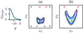
Figure 1: Noise shaping. Left: Noise-shaping function with the parameters corresponding to a 2D posterior and a maximum observed log-density $y_{\text{max}}=0$, with $\lambda_{\sigma}=0.3$. Larger noise $\sigma_{\text{shape}}$ is assigned to lower log-densities $y$. Right: Effect of noise-shaping on the inducing points (red) and the variational posterior $q_{\phi}$ for a $2D$ Rosenbrock function, for an underlying dense grid of training points; (a) without noise-shaping, (b) with noise-shaping. Noise-shaping affords a better representation of the region of interest with a limited number of inducing points.

Given a limited number of inducing points, we want the sparse GP representation to focus on high posterior density regions and allocate fewer resources to low-density regions. To achieve this goal, we introduce noise shaping as a simple motivated heuristic (see Fig. 1). Namely, we add artificial ‘shaping’ noise $\sigma_{\text{shape}}(y)$ (assumed Gaussian and independent) to the Gaussian likelihood of each observation in the model, without changing the actual observation $y$, that is:

$$\sigma^{2}_{\text{tot}}(\mathbf{x}_{n},y_{n}) =\sigma^{2}_{\text{obs}}(\mathbf{x}_{n})+\sigma^{2}_{\text{shape}}(\Delta y_{n})$$

where $\sigma^{2}_{\text{obs}}(\mathbf{x}_{n})$ is the estimated measurement variance at $\mathbf{x}_{n}$ ($\sigma^{2}_{\text{obs}}=10^{-5}$ for noiseless targets), $\Delta y_{n}\equiv y_{\text{max}}-y_{n}$, with $y_{\text{max}}$ the maximum observed log-density, and

$$\sigma^{2}_{\text{shape}}(\Delta y) =\exp\left\{(1-\rho)\log\sigma^{2}_{\text{min}}+\rho\log\sigma^{2}_{\text{med}}\right\}+\left[\mathbf{1}_{\Delta y\geq\theta_{\sigma}}\right]{\lambda_{\sigma}}^{2}(\Delta y-\theta_{\sigma})^{2},$$

where $\rho=\min(1,\Delta y/\theta_{\sigma})$; $\theta_{\sigma}$ is a threshold for ‘very low density’ points, at which we start the linear increase; $\lambda_{\sigma}$ is the slope of the increase; and $\sigma^{2}_{\text{min}}=10^{-3}$ and $\sigma^{2}_{\text{med}}=1$ are two shape parameters. Note that the added variance depends on $y_{n}$, the observation at $\mathbf{x}_{n}$. We chose $\sigma^{2}_{\text{shape}}(\Delta y)$ to add very small noise to relatively high-valued observations of the log-density, and increasingly larger noise to lower-density points; see Fig. 1 (left) and Appendix B.3 for further discussion. In practice, introducing noise-shaping leads to better positioned inducing points and better posterior estimation. In Fig. 1 (right), we show on a toy example how noise shaping clearly guides the placement of inducing points in regions of interest of the target ‘banana’ function (the training set, not shown, is a dense regular grid).

As further motivation, we show that noise shaping is equivalent to downweighing observations in the sparse GP objective of sgpr. The GP observation likelihood becomes

$$\log\tilde{p}(\mathbf{y}\mid\mathbf{f})=C-\sum_{n=1}^{N}\frac{(y_{n}-f(\mathbf{x}_{n}))^{2}}{2\sigma^{2}_{\text{tot}}(\mathbf{x}_{n},y_{n})}$$

where $C=-\sum_{n}\log\sqrt{2\pi\sigma^{2}_{\text{tot}}(\mathbf{x}_{n},y_{n})}$ is a constant that does not depend on the GP $\mathbf{f}$. Using the expression for the ‘uncollapsed’ sparse GP objective from [Hensman et al., 2015], we obtain the following expression for the expected log-likelihood term of the GP-elbo,

$$\mathbb{E}_{q(\mathbf{f})}[\log\tilde{p}(\mathbf{y}\mid\mathbf{f})]=C+\sum_{n=1}^{N}w_{n}\mathbb{E}_{q(f_{n})}[\log p(y_{n}|f_{n})],$$

where $q(\mathbf{f})$ is the variational GP posterior and $w_{n}\equiv\sigma^{2}_{\text{obs}}(\mathbf{x}_{n})/\sigma^{2}_{\text{tot}}(\mathbf{x}_{n},y_{n})\leq 1$. In sum, by assigning larger ‘shaping’ noise to low-density observations we are downweighing their role in the sparse GP representation, guiding the sparse GP to better represent higher-density regions.

4 THEORETICAL RESULTS

In this section, we present two theoretical results in support of the consistency and validity of the sparse approximation used in svbmc. Proofs are given in Appendix D.

Our first results are related to the convergence of the sparse GP surrogate towards the true (unnormalized) target log posterior $f_{0}$ under acquisitions of new points using the acquisition functions from Section 3.4. Due to their different form, we treat each function separately. Acquisition function $a_{1}$ belongs to a class of acquisition functions for adaptive Bayesian quadrature whose convergence is proved by Kanagawa and Hennig [2019]. In Appendix D, we show that these convergence results can be adapted to the sparse GP case. Acquisition function $a_{2}$ is more complex due to the integral form. We recall that the aim of $a_{2}$ is to minimize the variational integrated median interquantile range, $\mathcal{L}=\int_{\mathcal{X}}q_{\phi}(\mathbf{x})\mathrm{sinh}(\alpha s(\mathbf{x}))\mathrm{d}\mathbf{x}$. $a_{2}$ achieves so by one-step lookahead, i.e., by computing the expected reduction in such quantity after evaluating a candidate point. In Theorem 4.1, we show that the approximation error between the sgpr posterior and the true posterior is bounded by $\mathcal{L}$. In other words, by minimizing this loss, $a_{2}$ will also improve the sparse GP approximation towards the true posterior.

Theorem 4.1.

Assume $\mathcal{X}$ is compact and that the variances of the components in $q_{\phi}$ are bounded from below by $\sigma_{0}$. Let $h$ be a $\mathcal{C}^{1}$ function of $X$, then there exists a constant $C$ depending only on $\mathcal{X}$, $f_{0}$, $h$ and $\sigma_{0}$ such that:

$$\textstyle\left|\int h(\mathbf{x})\mathrm{exp}(\bar{f}(\mathbf{x}))\mathrm{d}\mathbf{x}-\int h(\mathbf{x})\mathrm{exp}(f_{0}(\mathbf{x}))\mathrm{d}\mathbf{x}\right|\leq C\int q_{\phi}(\mathbf{x})\mathrm{sinh}(\alpha s(\mathbf{x}))\mathrm{d}\mathbf{x}.$$

The previous results do not deal with the variational posterior $q_{\phi}$ which is the main output of svbmc. In our second result, we show that the sparse approximation introduced by svbmc does not induce arbitrarily large errors in the variational posterior $q_{\phi}$, compared to what we would obtain with an exact GP (e.g., as in vbmc). Theorem 4.2 shows that the distance between the variational posterior $q_{\phi}$ from svbmc and one obtained under an exact GP in vbmc ($q_{\phi_{\textsc{vbmc}}}$) is bounded by the approximation errors of the algorithms.

Theorem 4.2.

Let $f_{\textsc{vbmc}}$ be the vbmc approximation of $f_{0}$, and $q_{\phi_{\textsc{vbmc}}}$ the variational posterior from vbmc. Let $\pi$ be the normalized posterior density associated with $\exp(f)$ (resp., $\pi_{\textsc{vbmc}}$ and $\exp(f_{\textsc{vbmc}})$). Assume that $\text{KL}(q_{\phi}\|\pi)<\gamma_{1}$ and $\text{KL}(q_{\phi_{\textsc{vbmc}}}\|\pi_{\textsc{vbmc}})<\gamma_{2}$, then there exist constants $K_{\mathrm{e}}$ and $\gamma$ (for a fixed sparse GP posterior), such that:

$$\|q_{\phi}-q_{\phi_{\textsc{vbmc}}}\|_{TV}<\sqrt{\gamma_{1}/2}+\sqrt{\gamma_{2}/2}+(1-\mathrm{exp}(-2K_{\mathrm{e}}\sqrt{\gamma/2})).$$

5 EXPERIMENTS

We now demonstrate the performance of our method on several challenging synthetic and real-world problems. Each problem is represented by a target posterior density assumed to be a black box. In particular, gradients are unavailable and evaluations of the log-density may be (mildly) expensive and possibly noisy. Further details and results of the experiments can be found in Appendix E. Source code will be made available at https://github.com/pipme/svbmc.

Procedure

For each problem, we allocate a budget of 5-12k target evaluations for the initial evaluations (see each problem’s description). We then grant a smaller additional budget for post-processing, denoted with $N_{f}$. The idea is that the initial evaluations can be run in parallel, possibly on multiple machines, whereas the final post-processing step is run on a single computer. Given the black-box setting, the initial evaluations come from either multiple runs of a popular derivative-free optimization algorithm (cma-es; Hansen et al., 2003) or multiple chains of a robust derivative-free mcmc method (slice sampling; Neal, 2003). Note that all target posterior evaluations are used to build the initial set (e.g., not just the output samples of slice sampling, but also all the auxiliary evaluations).

Algorithms

We compare svbmc to other methods that afford post-process, black-box estimation of the posterior within a few thousand target evaluations in total. The state-of-the-art method for post-process inference is Bayesian stacking [Yao et al., 2022], which combines unconverged runs of inference algorithms such as mcmc using importance reweighting. Yao et al. [2022] does not use active learning and is only applicable to settings with exact likelihoods. A strong contender for ‘cheap’ post-process inference is the Laplace approximation, obtained by computing a multivariate normal approximation of the posterior centered at the mode found by previous optimization runs for MAP estimation. Finally, we perform direct inference with a black-box mcmc method (slice sampling), with the same budget of function evaluations allocated for the initial evaluations.

Metrics

To assess the quality of the posterior approximation, we compute the mean marginal total variation distance (MMTV) and “Gaussianized” symmetrized KL divergence (gsKL) between the approximate and the true posterior. We also report the absolute difference between the true and estimated log marginal likelihood ($\Delta$LML). For each method, we also report the number $N_{f}$ of post-process function evaluations used. For Laplace, this corresponds to the evaluations used for numerical calculation of the Hessian. Bayesian stacking and mcmc do not use further post-process evaluations. See Appendix E for an extended definition of these metrics. For each metric, we report the median and bootstrapped 95% CI of the median over 20 runs.

5.1 Multivariate Rosenbrock-Gaussian

We begin our experiments with complex synthetic targets of known shape to demonstrate the flexibility and robustness of our algorithm. Here we consider a target likelihood in $D=6$ which consists of two Rosenbrock (banana) functions $\mathcal{R}(x,y)$ and a two-dimensional normal density. We apply a Gaussian prior to all dimensions. The target density is thus:

$$p(\mathbf{x})\propto e^{\mathcal{R}(x_{1},x_{2})}e^{\mathcal{R}(x_{3},x_{4})}\mathcal{N}(x_{5},x_{6};\mathbf{0},\mathbb{I})\mathcal{N}(\mathbf{x};\mathbf{0},3^{2}\mathbb{I})$$

where $\mathcal{R}(x_{1},x_{2})=-(x_{1}^{2}-x_{2})^{2}-\frac{(x_{2}-1)^{2}}{100}$. The initial set consists of $5000$ total evaluations from multiple runs of cma-es with random starting points.

To check the robustness of svbmc to bad choices of initial samples, we then consider a truncated initial set where all the points with $x_{1}>0$ have been removed. Thanks to active sampling, svbmc can easily reconstruct the missing half of the distribution, converging after only a few more evaluations compared to the full set (Fig. 2). Table 1 presents results for the full and truncated initial sets, showing good performance of our method on this complex target.

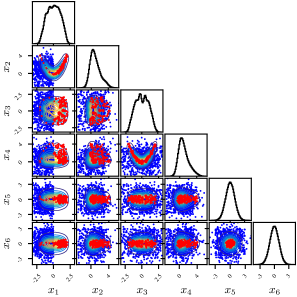
Figure 2: Multivariate Rosenbrock-Gaussian (truncated set). Example svbmc result for multivariate Rosenbrock-Gaussian with truncated initial samples. Blue points represent initial truncated cma-es samples (points with $x_{1}>0$ removed) and red points represent newly acquired samples with active sampling. Within a few dozen evaluations, svbmc is able to fully reconstruct the true target.

Table 1: Multivariate Rosenbrock-Gaussian ($D=6$)

	$\Delta$LML	MMTV	gsKL	$N_{f}$
svbmc Full	0.26 $\scriptstyle[0.23,0.27]$	0.086 $\scriptstyle[0.084,0.088]$	0.12 $\scriptstyle[0.095,0.12]$	200
svbmc Truncated	0.23 $\scriptstyle[0.22,0.26]$	0.083 $\scriptstyle[0.082,0.088]$	0.11 $\scriptstyle[0.086,0.13]$	200
Laplace	1.3	0.27	5.2	1081
mcmc	0.36 $\scriptstyle[0.25,0.45]$	0.12 $\scriptstyle[0.11,0.13]$	0.37 $\scriptstyle[0.26,0.55]$	–

5.2 Two moons bimodal posterior

To evaluate how our method copes with multimodality, we consider a synthetic bimodal posterior consisting of two ‘moons’ with different weights in $D=2$ (Fig. 3).

The initial samples come from short mcmc runs with 4 chains, for 250 evaluations each. The short chains rarely get a chance to swap modes, making it challenging for standard methods to assess the relative weight of each mode. As shown in Table 2, our method reconstructs the bimodal target almost perfectly. By contrast, both mcmc and in particular the Laplace approximation struggle with the bimodal posterior, despite its otherwise relative simplicity (Fig. 3).

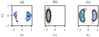
Figure 3: Visualization of two moons posterior: (a) mcmc samples. (b) Laplace approximation. (c) svbmc posterior.

Table 2: Two Moons posterior ($D=2$)

	$\Delta$LML	MMTV	gsKL	$N_{f}$
svbmc mcmc	0.0058 $\scriptstyle[0.0029,0.0083]$	0.021 $\scriptstyle[0.020,0.025]$	0.00048 $\scriptstyle[0.00034,0.00093]$	200
Laplace	0.42	0.19	15	121
mcmc	0.26 $\scriptstyle[0.13,0.29]$	0.12 $\scriptstyle[0.094,0.13]$	0.059 $\scriptstyle[0.032,0.098]$	–

5.3 Lotka-Volterra (LV) model

We consider inference for the Lotka-Volterra model of predatory-prey population dynamics, where $u(t)$ is the population size of the preys at time $t$, and $v(t)$ of the predators [Carpenter, 2018]. We assume noisy observations, with noise intensity $\sigma_{u}$ and $\sigma_{v}$, of the ODE

$$\frac{\mathrm{d}u}{\mathrm{d}t}=\alpha u-\beta uv;\quad\frac{\mathrm{d}v}{\mathrm{d}t}=-\gamma v+\delta uv;$$

with data coming from Howard [2009]. We aim to infer the posterior over model parameters $\mathbf{x}\equiv(\alpha,\beta,\gamma,\delta,u(0),v(0),\sigma_{u},\sigma_{v})$, with $D=8$. We use a closed-form likelihood derived from a finite element approximation of the equations [Carpenter, 2018]. We tested our method with two different initial sets of points: $5000$ evaluations of cma-es; or short mcmc runs of $4$ chains with a budget of 3000 function evaluations each. The results are presented in Table 3. While the performance of svbmc is slightly influenced by the source of the samples, our method with either initial set provides substantially better posterior approximations than Bayesian stacking, Laplace, or mcmc alone. Notably, svbmc is also cheaper than the Laplace approximation in terms of post-process function evaluations.

Table 3: Lotka-Volterra Model ($D=8$)

	$\Delta$LML	MMTV	gsKL	$N_{f}$
svbmc mcmc	0.17 $\scriptstyle[0.14,0.20]$	0.053 $\scriptstyle[0.048,0.064]$	0.15 $\scriptstyle[0.094,0.17]$	200
svbmc cma-es	0.11 $\scriptstyle[0.081,0.14]$	0.053 $\scriptstyle[0.048,0.057]$	0.12 $\scriptstyle[0.10,0.13]$	200
Laplace	0.45	0.082	0.59	1921
mcmc	1.1 $\scriptstyle[0.78,2.2]$	0.24 $\scriptstyle[0.18,0.27]$	2.5     $\scriptstyle[1.7,4.1]$	–
[Yao et al., 2022]	0.58 $\scriptstyle[0.50,0.74]$	0.24 $\scriptstyle[0.20,0.30]$	2.6     $\scriptstyle[2.2,3.5]$	–

5.4 Bayesian timing model

We consider a popular model of Bayesian time perception from cognitive neuroscience [Acerbi et al., 2012]. The model has $D=5$ parameters representing properties of the Bayesian observer (sensory and motor noise, etc.); see Appendix E.2.4 for a detailed description. We infer the posterior of a representative subject from Acerbi et al. [2012] in two different inference scenarios: one of noiseless target evaluations (obtained through a closed-form solution of the likelihood); and one assuming noisy evaluations of the log-likelihood, such as those obtained via simulator-based estimation [van Opheusden et al., 2020]. For noisy evaluations we set the standard deviation $\sigma_{\text{obs}}=5$, which corresponds to substantial estimation noise in log-likelihood space [Acerbi, 2020].

The initial sample consists of $5000$ evaluations from cma-es, activating a noise-handling feature as needed [Hansen et al., 2009]. The results are presented in Table 4 and Fig. 4. Notably, our method outperforms the Laplace approximation, mcmc and Bayesian stacking even in the case of noisy observations of the target, which the other algorithms cannot handle (e.g., numerical estimation of a noisy Hessian is nontrivial, and mcmc or importance reweighting with noisy log-density evaluations is also problematic). We also found that noisy evaluations can lead to better performance of svbmc on some metrics, possibly due to wider exploration of cma-es with a noisy target.

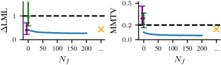
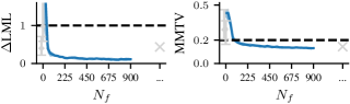
Figure 4: Performance on Timing posterior: $\Delta$LML loss (left) and MMTV (right) as a function of the number of post-processing function calls for the Bayesian Timing model. Top: Exact likelihood evaluations. Blue curve is svbmc, the orange cross represents the Laplace approximation, the green dot the mcmc approximation, and the purple diamond Bayesian stacking (with 95% confidence intervals). Bottom: Noisy likelihood evaluations. Only svbmc (blue) supports noisy likelihood evaluations. The performance of the other methods is shown there (light grey) only for reference, copied from the exact case.

Table 4: Bayesian Timing Model ($D=5$)

	$\Delta$LML	MMTV	gsKL	$N_{f}$
svbmc noiseless	0.27 $\scriptstyle[0.26,0.27]$	0.057 $\scriptstyle[0.055,0.058]$	0.093 $\scriptstyle[0.083,0.097]$	200
svbmc noisy	0.11 $\scriptstyle[0.07,0.14]$	0.13 $\scriptstyle[0.12,0.14]$	0.14 $\scriptstyle[0.12,0.16]$	900
Laplace	0.43	0.14	1.4	751
mcmc	0.98 $\scriptstyle[0.58,1.8]$	0.29 $\scriptstyle[0.16,0.37]$	18        $\scriptstyle[10,29]$	–
[Yao et al., 2022]	0.40 $\scriptstyle[0.22,0.71]$	0.29 $\scriptstyle[0.21,0.46]$	9.5     $\scriptstyle[7.3,18]$	–

6 RELATED WORK

We review here other related work, beyond the immediately related background work covered in Section 2.

Besides vbmc, our work is related to the literature on GP-based methods for estimation of the posterior [Rasmussen, 2003, Kandasamy et al., 2015, Wang and Li, 2018, Järvenpää et al., 2021] and on adaptive Bayesian quadrature [Osborne et al., 2012, Gunter et al., 2014, Chai and Garnett, 2019]. These methods, being based on exact GPs, are not directly applicable to our setting of many thousand evaluations. Our results on sparse Bayesian quadrature (Section 3.3) and acquisition functions with sparse GPs (Section 3.4), though, may be useful to extend other GP-based inference techniques to the sparse case.

The setting of parallel runs followed by a centralized post-processing step is reminiscent of embarrassingly parallel mcmc techniques [Neiswanger et al., 2013], some of which also make use of GP surrogates [Nemeth and Sherlock, 2018] and active learning [De Souza et al., 2022]. However, embarrassingly parallel methods require a specific setup for the parallel runs (i.e., splitting data into partitions), which is incompatible with the purely post-process philosophy (modulo a few extra evaluations) of svbmc.

Yao et al. [2022] propose to reuse parallel – and possibly incomplete – runs of different inference algorithms by combining them in a weighted average via ‘Bayesian stacking’. Crucially, the computation of the stacking weights only requires a post-processing step. Unlike our method, Bayesian stacking does not make use of all available target evaluations, and has no built-in technique, like active sampling, to correct for mistakes in the stacked approximation, which makes it perform worse in our experiments than svbmc.

Finally, noise shaping (Section 3.5) is similar in spirit to the weighted KL divergence method proposed by McIntire et al. [2016] in the context of Bayesian optimization with sparse GPs. The key difference is that noise shaping effectively downweighs the observations, whereas the KL approach applies a weighting function when evaluating the KL divergence between the sparse and exact GP posteriors. In practice, noise shaping is easy to implement with a heteroskedastic Gaussian likelihood and it is plug-and-play with sgpr, while the weighted KL method is more involved.

7 DISCUSSION

In this paper, we proposed sparse Variational Bayesian Monte Carlo (svbmc) as a new method to perform post-process black-box Bayesian inference. By recycling evaluations from previous runs of other algorithms (e.g., optimizations, non-converged mcmc chains), svbmc affords full Bayesian inference at a limited additional cost. Our method produces good solutions within a few iterations of active sampling, as demonstrated on a series of challenging benchmarks, outperforming the current state-of-the-art while allowing for additional improvement of the posterior and more flexibility in the input. To our knowledge, svbmc is the first method that uses a large amount of previous posterior density evaluations as a basis for posterior estimation, with no limitation on the origin of these points. While our results show the promise of svbmc for post-process Bayesian inference, several aspects remain open for future research.

7.1 Limitations and future work

Our method shares with other GP-based surrogate models (see Section 6) the issue of scalability to a higher dimension (above $\sim 10$). While the ability of svbmc to handle a larger number of evaluations might expand the range of tractable dimensions, it is unlikely to fully solve an intrinsic problem of simple kernel methods. More flexible kernels [Wilson and Adams, 2013] or different surrogate models, like deep networks, might be the key to broader scalability.

Noise shaping, a principled heuristic introduced in Section 3.5, is an important component of svbmc. We chose the noise shaping function out of theoretical and empirical considerations, but further work is needed to make it a general tool for surrogate modelling, e.g., via adaptive techniques.

On the theory side, while we presented preliminary consistency results (Section 4), a full convergence analysis of svbmc that accounts for the convergence of both the (sparse) GP surrogate and the variational posterior represents an important future research direction.

Finally, in this work we used sgpr due to its numerical convenience (i.e., closed-form solutions for the sparse GP posterior) but sgpr is also somewhat limited in scalability and to Gaussian observations. A natural next step of our work would consist of extending svbmc to stochastic variational GPs (svgp; Hensman et al., 2013, 2015), which are able to handle nearly-arbitrarily large datasets and non-Gaussian observations of the target density.

Appendix

In this Appendix, we include mathematical proofs, implementation details, additional results, and extended explanations omitted from the main text. An implementation of the svbmc algorithm in the paper will be made available at https://github.com/pipme/svbmc.

Appendix A Background information

We provide here background information on the building blocks of the svbmc algorithm, from variational inference to (sparse) Gaussian processes and Bayesian quadrature, and finally the vbmc framework. This section follows previous work on vbmc, Gaussian process surrogate modelling and active learning (e.g., Acerbi, 2020, De Souza et al., 2022).

A.1 Variational inference

Let $\mathbf{x}\in\mathcal{X}\subseteq\mathbb{R}^{D}$ be a parameter vector of a model of interest, and $\mathcal{D}$ a dataset. Variational inference approximates the intractable posterior $p(\mathbf{x}|\mathcal{D})$ via a simpler distribution $q(\mathbf{x})\equiv q_{\bm{\phi}}(\mathbf{x})$ that belongs to a parametric family indexed by $\bm{\phi}$ [Jordan et al., 1999, Bishop, 2006]. The goal of variational inference is to find $\bm{\phi}$ for which the variational posterior $q_{\bm{\phi}}$ is “closest” in approximation to the true posterior, as quantified by the Kullback-Leibler (KL) divergence,

$$D_{\text{KL}}\left[q_{\bm{\phi}}(\mathbf{x})||p(\mathbf{x}|\mathcal{D})\right]=\mathbb{E}_{\bm{\phi}}\left[\log\frac{q_{\bm{\phi}}(\mathbf{x})}{p(\mathbf{x}|\mathcal{D})}\right],$$ (S1)

where $\mathbb{E}_{\bm{\phi}}\equiv\mathbb{E}_{q_{\bm{\phi}}}$. Crucially, $D_{\text{KL}}(q||p)\geq 0$ and the equality is achieved if and only if $q\equiv p$. Minimizing the KL divergence casts Bayesian inference as an optimization problem, which can be shown equivalent to finding the variational parameter vector $\bm{\phi}$ that maximizes the following objective,

$$\text{{elbo}}\left[q_{\bm{\phi}}\right]=\mathbb{E}_{\bm{\phi}}\left[\log\frac{p(\mathcal{D}|\mathbf{x})p(\mathbf{x})}{q_{\bm{\phi}}(\mathbf{x})}\right]=\mathbb{E}_{\bm{\phi}}\left[f(\mathbf{x})\right]+\mathcal{H}[q_{\bm{\phi}}(\mathbf{x})],$$ (S2)

with $f(\mathbf{x})\equiv\log p(\mathcal{D}|\mathbf{x})p(\mathbf{x})=\log p(\mathcal{D},\mathbf{x})$ the log joint probability, and $\mathcal{H}[q]$ the entropy of $q$. Eq. S2 is the evidence lower bound (elbo), a lower bound to the log marginal likelihood or model evidence, since elbo $[q_{\bm{\phi}}]\leq\log p(\mathcal{D})$, with equality holding if $q(\mathbf{x})\equiv p(\mathbf{x}|\mathcal{D})$.

In our setting, $f(\mathbf{x})$ is a potentially expensive or noisy black-box function (in particular, no gradients), which prevents a direct maximization of Eq. S2 via Monte Carlo or standard stochastic gradient techniques (e.g., Ranganath et al., 2014).

A.2 Gaussian processes

Gaussian processes (GPs) are a flexible class of statistical models for specifying prior distributions over unknown functions $f:\mathcal{X}\subseteq\mathbb{R}^{D}\rightarrow\mathbb{R}$ [Rasmussen and Williams, 2006]. In this paper, GPs are used as surrogate models for unnormalized log-posteriors, for which we use the model presented in this section. We recall that GPs are defined by a positive definite covariance, or kernel function $\kappa:\mathcal{X}\times\mathcal{X}\rightarrow\mathbb{R}$; a mean function $m:\mathcal{X}\rightarrow\mathbb{R}$; and a likelihood or observation model.

Kernel function.

We use the common squared exponential or Gaussian kernel,

$$\kappa(\mathbf{x},\mathbf{x}^{\prime};\sigma_{f}^{2},\bm{\ell})=\sigma_{f}^{2}\exp\left[-\frac{1}{2}\left(\mathbf{x}-\mathbf{x}^{\prime}\right)\mathbf{\Sigma}_{\ell}^{-1}\left(\mathbf{x}-\mathbf{x}^{\prime}\right)^{\top}\right]\qquad\text{with}\;\mathbf{\Sigma}_{\ell}=\text{diag}\left[\ell_{1}^{2},\ldots,\ell_{D}^{2}\right],$$ (S3)

where $\sigma_{f}$ is the output scale and $\bm{\ell}\equiv(\ell_{1},\ldots,\ell_{D})$ is the vector of input length scales. This choice of kernel affords closed-form expressions for Bayesian quadrature (see below).

Mean function.

Following vbmc [Acerbi, 2018, 2019], we use a negative quadratic mean function such that the surrogate posterior (i.e., the exponentiated surrogate log-posterior) is integrable. A negative quadratic can be interpreted as a prior assumption that the target posterior is a multivariate normal; but note that the GP can model deviations from this assumption and represent multimodal distributions as well (see for example the two moons problem in the main text and Section E.2.2). In this paper, we use

$$m(\mathbf{x};m_{0},\bm{\mu},\bm{\omega})\equiv m_{0}-\frac{1}{2}\sum_{i=1}^{D}\frac{\left(x_{i}-\mu_{i}\right)^{2}}{\omega_{i}^{2}},$$ (S4)

where $m_{0}$ denotes the maximum, $\bm{\mu}\equiv\left(\mu_{1},\ldots,\mu_{D}\right)$ is the location vector, and $\bm{\omega}\equiv\left(\omega_{1},\ldots,\omega_{D}\right)$ is a vector of length scales.

Observation model.

Finally, GPs are also characterized by a likelihood or observation noise model. In this paper, we consider both noiseless and noisy evaluations of the target log-posterior. For noiseless targets, we use a Gaussian likelihood with a small variance $\sigma_{\text{obs}}^{2}=10^{-5}$ for numerical stability. Noisy evaluations of the target often arise from stochastic estimation of the log-likelihood via simulation [Wood, 2010, van Opheusden et al., 2020]. For noisy targets, we assume the observation variance $\sigma_{\text{obs}}^{2}(\mathbf{x}_{n})$ at each training input location $\mathbf{x}_{n}$ is given (e.g., estimated via bootstrap or other means). Due to noise shaping (see below), for both noiseless and noisy targets we end up with a heteroskedastic Gaussian observation noise model, in which the variance can vary from point to point. We denote with $\mathbf{D}$ the diagonal matrix of observation noise, with $\mathbf{D}\equiv\text{diag}\left[\sigma_{\text{obs}}^{2}(\mathbf{x}_{1}),\ldots,\sigma_{\text{obs}}^{2}(\mathbf{x}_{N})\right]$.

Hyperparameters.

The GP hyperparameters are represented by a vector $\bm{\xi}\equiv\left(\sigma_{f},\bm{\ell},m_{0},\bm{\mu},\bm{\omega}\right)$ which collects the GP covariance and mean hyperparameters.

Inference.

Conditioned on training inputs $\mathbf{X}=\left\{\mathbf{x}_{1},\ldots,\mathbf{x}_{N}\right\}$, observed function values $\mathbf{y}$, observed noise $\mathbf{D}\equiv\text{diag}\left[\sigma_{\text{obs}}^{2}(\mathbf{x}_{1}),\ldots,\sigma_{\text{obs}}^{2}(\mathbf{x}_{N})\right]$ and GP hyperparameters $\bm{\xi}$, the posterior GP mean and covariance are available in closed form [Rasmussen and Williams, 2006],

$$\begin{split}\overline{f}_{\mathbf{X},\mathbf{y},\mathbf{D}}(\mathbf{x})\equiv\mathbb{E}\left[f(\mathbf{x})|\mathbf{X},\mathbf{y},\mathbf{D},\bm{\xi}\right]=&\;\kappa(\mathbf{x},\mathbf{X})\left[\mathbf{K}_{\mathbf{X},\mathbf{X}}+\mathbf{D}\right]^{-1}(\mathbf{y}-m(\mathbf{X}))+m(\mathbf{x})\\ C_{\mathbf{X},\mathbf{y},\mathbf{D}}(\mathbf{x},\mathbf{x}^{\prime})\equiv\text{Cov}\left[f(\mathbf{x}),f(\mathbf{x}^{\prime})|\mathbf{X},\mathbf{y},\mathbf{D},\bm{\xi}\right]=&\;\kappa(\mathbf{x},\mathbf{x}^{\prime})-\kappa(\mathbf{x},\mathbf{X})\left[\mathbf{K}_{\mathbf{X},\mathbf{X}}+\mathbf{D}\right]^{-1}\kappa(\mathbf{X},\mathbf{x}^{\prime}),\end{split}$$ (S5)

where $\mathbf{K}_{\mathbf{X},\mathbf{X}}$ denotes the GP kernel matrix $\kappa(\mathbf{x},\mathbf{x}^{\prime})$ evaluated at every pair of points $(\mathbf{x},\mathbf{x}^{\prime})\in\mathbf{X}\times\mathbf{X}$.

Training.

Training a GP means finding the hyperparameters that best represent a given dataset of input points, function observations and noise $\left(\mathbf{X},\mathbf{y},\mathbf{D}\right)$. In this paper, we train the exact GP models by maximizing the log marginal likelihood of the GP plus a log-prior term that acts as regularizer, a procedure known as maximum-a-posteriori estimation. Thus, the training objective to maximize is

$$\begin{split}\log p(\bm{\xi}|\mathbf{X},\mathbf{y},\mathbf{D})=&-\frac{1}{2}\left(\mathbf{y}-m(\mathbf{X};\bm{\xi})\right)^{\top}\left[\kappa(\mathbf{X},\mathbf{X};\bm{\xi})+\mathbf{D}\right]^{-1}\left(\mathbf{y}-m(\mathbf{X};\bm{\xi})\right)\\ &+\frac{1}{2}\log\det\left(\kappa(\mathbf{X},\mathbf{X};\bm{\xi})+\mathbf{D}\right)+\log p(\bm{\xi})+\text{const},\end{split}$$ (S6)

where $p(\bm{\xi})$ is the prior over GP hyperparameters. We used the same prior over GP hyperparameters as recent versions of vbmc, as defined in Acerbi [2020, Supplementary Material, Section B.1].

A.3 Sparse Gaussian process regression

The computational cost associated with exact GP process training (see Section A.2) is typically of the order $\mathcal{O}(N^{3})$, which does not cope well with a large number of observations. A better scaling can be obtained via the use of so-called sparse Gaussian Processes (e.g., Titsias, 2009, Hensman et al., 2015). The general idea is based upon the inducing point method [Snelson and Ghahramani, 2005], which introduces $\mathbf{Z}$ and $\mathbf{u}$, known respectively as inducing inputs and inducing variables. In short, we aim to build an approximate GP defined on the inducing points $\mathbf{Z}\equiv\left(\mathbf{z}_{1},\ldots,\mathbf{z}_{M}\right)$ and values $\mathbf{u}$ which best approximates the full GP, for $M\ll N$. We do so by first assuming that values $\mathbf{u}$ are the results of the same Gaussian process as $\mathbf{f}$, so we can write their joint distribution as a multivariate Gaussian distribution (for simplicity, here in the zero-mean case):

$$p(\mathbf{f},\mathbf{u})=\mathcal{N}\left(\cdot\left|\,\mathbf{0},\left[\begin{pmatrix}\mathbf{K}_{\mathbf{X},\mathbf{X}}&\mathbf{K}_{\mathbf{X},\mathbf{Z}}\\ \mathbf{K}_{\mathbf{Z},\mathbf{X}}&\mathbf{K}_{\mathbf{Z},\mathbf{Z}}\end{pmatrix}\right]\right.\right),$$

where $\mathbf{K}_{\mathbf{Z},\mathbf{X}}$ and $\mathbf{K}_{\mathbf{X},\mathbf{Z}}$ are the cross-covariance matrices for the GP prior evaluated at the points in $\mathbf{X}$ and $\mathbf{Z}$.

In turn, we can seek to write the full posterior $p(\mathbf{y},\mathbf{f},\mathbf{u})$ as a variational posterior [Titsias, 2009]:

$$p(\mathbf{y},\mathbf{f},\mathbf{u})=p(\mathbf{y}\mid\mathbf{f})p(\mathbf{f}\mid\mathbf{u})p(\mathbf{u}),$$

and find the best distribution in the KL-divergence sense for $p(\mathbf{u})$. For the case of sparse GP regression (sgpr) with Gaussian likelihood, Titsias [2009] proved that the optimal variational distribution is $\tilde{p}(\mathbf{u})=\mathcal{N}(\mathbf{m}_{\mathbf{u}},\mathbf{S}_{\mathbf{u}\mathbf{u}})$, and that equality between the sparse and full posterior is obtained for $\mathbf{Z}=\mathbf{X}$. We denote with $\bm{\psi}$ the optimal variational parameters $\mathbf{m}_{\mathbf{u}},\mathbf{S}_{\mathbf{u}\mathbf{u}}$ of the sparse GP, defined as:

$$\mathbf{m}_{\mathbf{u}} =\mathbf{K}_{\mathbf{Z},\mathbf{Z}}\bm{\Sigma}\mathbf{K}_{\mathbf{Z},\mathbf{X}}\mathbf{\mathbf{D}}^{-1}\mathbf{y},$$ (S7)

$$\mathbf{S}_{\mathbf{u}\mathbf{u}} =\mathbf{K}_{\mathbf{Z},\mathbf{Z}}\bm{\Sigma}\mathbf{K}_{\mathbf{Z},\mathbf{Z}},$$ (S8)

where $\bm{\Sigma}\equiv(\mathbf{K}_{\mathbf{Z},\mathbf{X}}\mathbf{\mathbf{D}}^{-1}\mathbf{K}_{\mathbf{X},\mathbf{Z}}+\mathbf{K}_{\mathbf{Z},\mathbf{Z}})^{-1}$.

sgpr posterior.

The sgpr posterior is also a Gaussian process with mean and covariance:

$$\mu_{\bm{\psi}}(\tilde{\mathbf{x}}) =\kappa(\tilde{\mathbf{x}},\mathbf{Z})\bm{\Sigma}\mathbf{K}_{\mathbf{Z},\mathbf{X}}\mathbf{D}^{-1}\mathbf{y},$$ (S9)

$$\kappa_{\bm{\psi}}(\tilde{\mathbf{x}},\tilde{\mathbf{x}}^{\prime}) =\kappa(\tilde{\mathbf{x}},\tilde{\mathbf{x}}^{\prime})-\kappa(\tilde{\mathbf{x}},\mathbf{Z})(\mathbf{K}_{\mathbf{Z},\mathbf{Z}}^{-1}-\bm{\Sigma})\kappa(\mathbf{Z},\tilde{\mathbf{x}}^{\prime}).$$ (S10)

sgpr elbo.

The elbo in sgpr [Titsias, 2009], extended here to the heteroskedastic case, is:

$$\text{GP-{elbo}}(\mathbf{Z},\bm{\xi})=\log\mathcal{N}\left(\mathbf{y};\mathbf{m}_{\mathbf{u}},\mathbf{Q}_{\mathbf{X},\mathbf{X}}+\mathbf{D}\right)-\frac{1}{2}{\operatorname{Tr}}\left(\left(\mathbf{K}_{\mathbf{X},\mathbf{X}}-\mathbf{Q}_{\mathbf{X},\mathbf{X}}\right)\mathbf{\mathbf{D}}^{-1}\right),$$ (S11)

where $\mathbf{Q}_{\mathbf{X},\mathbf{X}}\equiv\mathbf{K}_{\mathbf{X},\mathbf{Z}}\mathbf{K}_{\mathbf{Z},\mathbf{Z}}^{-1}\mathbf{K}_{\mathbf{Z},\mathbf{X}}$. We refer to Eq.S11 as GP-elbo to differentiate it from the elbo of the variational approximation in vbmc and svbmc (see below). Note that the GP-elbo depends on the location of inducing points $\mathbf{Z}$ and GP hyperparameters $\bm{\xi}$, and consists of the log pdf of a multivariate normal term, as expected of a GP, minus the trace of an error term. For detailed derivations, refer to Section C.1.

A.4 Bayesian quadrature

Bayesian quadrature [O’Hagan, 1991, Ghahramani and Rasmussen, 2002a] is a technique to obtain Bayesian estimates of intractable integrals of the form

$$\mathcal{J}=\int_{\mathcal{X}}f(\mathbf{x})\pi(\mathbf{x})d\mathbf{x},$$ (S12)

where $f$ is a function of interest and $\pi$ a known probability distribution. Here we consider the domain of integration $\mathcal{X}=\mathbb{R}^{D}$. When a GP prior is specified for $f$, since integration is a linear operator, the integral $\mathcal{J}$ is also a Gaussian random variable whose posterior mean and variance are [Ghahramani and Rasmussen, 2002a]

$$\mathbb{E}_{f}[\mathcal{J}]=\int\overline{f}(\mathbf{x})\pi(\mathbf{x})d\mathbf{x},\qquad\mathbb{V}_{f}[\mathcal{J}]=\int\int C(\mathbf{x},\mathbf{x}^{\prime})\pi(\mathbf{x})\pi(\mathbf{x}^{\prime})d\mathbf{x}d\mathbf{x}^{\prime},$$ (S13)

where $\overline{f}$ and $C$ are the GP posterior mean and covariance from Eq. S5. Importantly, if $f$ has a Gaussian kernel and $\pi$ is a Gaussian or mixture of Gaussians (among other functional forms), the integrals in Eq. S13 have closed-form solutions.

A.5 Variational Bayesian Monte Carlo

Variational Bayesian Monte Carlo (vbmc) is a framework for sample-efficient inference [Acerbi, 2018, 2020]. Let $f=\log p(\mathcal{D}|\mathbf{x})p(\mathbf{x})$ be the target log joint probability (unnormalized posterior), where $p(\mathcal{D}|\mathbf{x})$ is the model likelihood for dataset $\mathcal{D}$ and parameter vector $\mathbf{x}\in\mathcal{X}\subseteq\mathbb{R}^{D}$, and $p(\mathbf{x})$ the prior. vbmc assumes that only a limited number of potentially noisy log-likelihood evaluations are available, up to several hundreds. vbmc works by iteratively improving a variational approximation $q_{\bm{\phi}}(\mathbf{x})$, indexed by $\bm{\phi}$, of the true target posterior density. In each iteration $t$, the algorithm:

1. Actively samples sequentially $n_{\text{active}}$ ‘promising’ new points, by iteratively maximizing a given acquisition function $a(\mathbf{x}):\mathcal{X}\rightarrow\mathbb{R}$; for each selected point $\mathbf{x}_{\star}$ evaluates the target $y_{\star}\sim f(\mathbf{x}_{\star})+\sigma_{\text{obs}}(\mathbf{x}_{\star})\varepsilon$, where $\sigma_{\text{obs}}(\mathbf{x}_{\star})$ is the observation noise at the point and $\varepsilon$ an i.i.d. standard normal random variable; $n_{\text{active}}=5$ by default.

2. Trains a GP surrogate model of the log joint $f$, given the training set $\left\{\mathbf{X}_{t},\mathbf{y}_{t},\mathbf{D}_{t}\right\}$ of input points, their associated observed values and observation noise so far.

3. Updates the variational posterior parameters $\bm{\phi}_{t}$ by optimizing the surrogate elbo (variational lower bound on the model evidence) calculated via Bayesian quadrature.

This loop repeats until reaching a termination criterion (e.g., budget of function evaluations or lack of improvement over several iterations), and the algorithm returns both the variational posterior and posterior mean and variance of the elbo. vbmc includes an initial warm-up stage to converge faster to regions of high posterior probability, before starting to refine the variational solution. We describe below basic features of vbmc; see Acerbi [2018, 2020] for more details.

Variational posterior.

The variational posterior is a flexible mixture of $K$ multivariate Gaussians,

$$q_{\bm{\phi}}(\mathbf{x})=\sum_{k=1}^{K}w_{k}\mathcal{N}\left({\mathbf{x}};{\bm{\mu}_{k}},{\sigma_{k}^{2}\mathbf{\Sigma}_{\bm{\lambda}}}\right),\qquad\mathbf{\Sigma}_{\bm{\lambda}}\equiv\text{diag}[{{\lambda}^{(1)}}^{2},\ldots,{\lambda^{(D)}}^{2}],$$

where $w_{k}$, $\bm{\mu}_{k}$, and $\sigma_{k}$ are, respectively, the mixture weight, mean, and scale of the $k$-th component; and $\bm{\lambda}$ a common length scale vector. For a given $K$, the variational parameter vector is $\bm{\phi}\equiv(w_{1},\ldots,w_{K},$ $\bm{\mu}_{1},\ldots,\bm{\mu}_{K},$ $\sigma_{1},\ldots,\sigma_{K},\bm{\lambda})$. $K$ is set adaptively; fixed to $K=2$ during warm-up, and then increasing each iteration if it leads to an improvement of the elbo (see below).

Gaussian process model.

In vbmc, the log joint $f$ is approximated by an exact GP surrogate model with a squared exponential kernel, a negative quadratic mean function, and a Gaussian likelihood (possibly heteroskedastic), as described in Section A.2.

The Evidence Lower Bound (elbo).

Using the GP surrogate model $f$, and for a given variational posterior $q_{\bm{\phi}}$, the posterior mean of the surrogate elbo (see Eq. S2) can be estimated as

$$\mathbb{E}_{f}\left[\text{{elbo}}(\bm{\phi})\right]=\mathbb{E}_{f}\left[\mathbb{E}_{\bm{\phi}}\left[f\right]\right]+\mathcal{H}[q_{\bm{\phi}}],$$ (S14)

where $\mathbb{E}_{f}\left[\mathbb{E}_{\bm{\phi}}\left[f\right]\right]$ is the posterior mean of the expected log joint under the GP model, and $\mathcal{H}[q_{\bm{\phi}}]$ is the entropy of the variational posterior. In particular, the expected log joint takes the form

$$\mathbb{E}_{\bm{\phi}}\left[f\right]=\int q_{\bm{\phi}}(\mathbf{x})f(\mathbf{x})d\mathbf{x}.$$ (S15)

The choice of variational family and GP representation of vbmc affords closed-form solutions for the posterior mean and variance of Eq. S15 (and of their gradients) by means of Bayesian quadrature (see Section A.4). The entropy of $q_{\bm{\phi}}$ and its gradient are estimated via simple Monte Carlo and the reparameterization trick [Kingma and Welling, 2013, Miller et al., 2017], such that Eq. S14 can be optimized via stochastic gradient ascent [Kingma and Ba, 2014].

Acquisition function.

During the active sampling stage, new points to evaluate are chosen sequentially by maximizing a given acquisition function $a(\mathbf{x}):\mathcal{X}\rightarrow\mathbb{R}$ constructed to represent useful search heuristics [Kanagawa and Hennig, 2019]. The standard acquisition function for vbmc is prospective uncertainty sampling [Acerbi, 2018, 2019] for noiseless targets and (variational) integrated median interquartile range [Acerbi, 2020, Järvenpää et al., 2021] for noisy targets. Non-integrated acquisition functions have been shown to perform very poorly with noisy targets [Acerbi, 2020, Järvenpää et al., 2021]. Kanagawa and Hennig [2019] proved convergence guarantees for active-sampling Bayesian quadrature under a broad class of pointwise acquisition functions.

Inference space.

The variational posterior and GP surrogate in vbmc are defined in an unbounded inference space equal to $\mathbb{R}^{D}$. Parameters that are subject to bound constraints are mapped to the inference space via a shifted and rescaled logit transform, with an appropriate Jacobian correction to the log-joint. Solutions are transformed back to the original space via a matched inverse transform, e.g., a shifted and rescaled logistic function for bound parameters [Carpenter et al., 2016, Acerbi, 2018].

Variational whitening.

The standard vbmc representation of both the variational posterior and GP surrogate is axis-aligned, which makes it ill-suited to deal with highly correlated posteriors. Variational whitening [Acerbi, 2020] deals with this issue by proposing a linear transformation of the inference space (a rotation and rescaling) such that the variational posterior $q_{\bm{\phi}}$ obtains unit diagonal covariance matrix. In vbmc, variational whitening is proposed a few iterations after the end of warm-up, and then at increasingly more distant intervals. A proposed whitening transformation is rejected if it does not yield an increase of the elbo. Acerbi [2020] showed the usefulness of whitening on complex, correlated posteriors.

Appendix B Algorithm details

We describe here additional details of features specific to the svbmc algorithm (see Section 3 in the main text). Further contributions used for the implementation of svbmc include several analytical derivations, reported later in Section C.

B.1 Trimming of the initial points

As mentioned in the main text, the trimming stage consists of removing from the initial set points with extremely low log posterior density, relative to the maximum observed value. The rationale is that such points are not particularly informative about the shape of the posterior and may instead induce numerical instabilities in the surrogate model.

Consider data point $\left(\mathbf{x}_{n},y_{n},\sigma_{n}\right)$, where $\sigma_{n}\equiv\sigma_{\text{obs}}(\mathbf{x}_{n})$ is the estimated standard deviation of the noise of the $n$-th observation. For each data point, we define the lower/upper confidence bounds of the log-density as, respectively, $\text{{lcb}}(\mathbf{x}_{n})\equiv y_{n}-\beta\sigma_{n}$, $\text{{ucb}}(\mathbf{x}_{n})\equiv y_{n}+\beta\sigma_{n}$, where $\beta>0$ is a confidence interval parameter. We trim all the points $\mathbf{x}_{n}$ for which

$$\text{{lcb}}_{\text{max}}-\text{{ucb}}(\mathbf{x}_{n})>\eta_{\text{trim}}$$

where $\text{{lcb}}_{\text{max}}=\max_{n}(\text{{lcb}}(\mathbf{x}_{n}))$. In other words, we trim all points whose difference in underlying log-density with the highest log-density is larger than a threshold with high probability (accounting for observation noise). In this paper, we use $\beta=1.96$, and $\eta_{\text{trim}}=20D$, with $D$ the dimension of the problem.

B.2 Selection of the inducing points

Inducing point location.

According to Burt et al. [2020], sampling from a $M$-determinantal point process ($M$-DPP) to select inducing points $\mathbf{Z}\subset\mathbf{X}$ will make the trace error term of the GP-elbo (see Eq. S11), close to its optimal value. In practice, we follow the recommendations in Burt et al. [2020] and Maddox et al. [2021] by sequentially selecting inducing points that greedily maximize the diagonal of the error term,

$$\mathbf{z}^{\star}=\arg\max_{\mathbf{z}}\text{diag}\left[\left(\mathbf{K}_{\mathbf{X},\mathbf{X}}-\mathbf{Q}_{\mathbf{X},\mathbf{X}}\right)\mathbf{D}^{-1}\right];$$ (S16)

in turn, this will minimize the trace error in Eq. S11. Eq. S16 can be interpreted as weighted greedy variance selection [Burt et al., 2020], in that it selects points with maximum prior conditional marginal variance at each point in $\mathbf{X}$ (conditioned on the inducing points selected so far), weighted by the precision (inverse variance) of the observation at that location.

Number of inducing points.

As a stopping criterion for choosing the number of inducing point $M=\left|\mathbf{Z}\right|$, we use the fractional error

$$\frac{\operatorname{Tr}\left(\left(\mathbf{K}_{\mathbf{X},\mathbf{X}}-\mathbf{Q}_{\mathbf{X},\mathbf{X}}\right)\mathbf{D}^{-1}\right)}{\operatorname{Tr}\left(\mathbf{K}_{\mathbf{X},\mathbf{X}}\mathbf{D}^{-1}\right)}<10^{-5}.$$

In this paper, for the experiments we also require $200\leq M\leq 300+2\sqrt{N_{f}}$, where $N_{f}$ is the number of additional target evaluations performed at post-processing time. We set these bounds to avoid selecting too few or too many inducing points, which can cause inferior performance in posterior approximation or problems in computational efficiency. Overall, this selection procedure can be achieved with complexity $\mathcal{O}(NM^{2})$ by Algorithm 1 in Chen et al. [2018].

GP hyperparameters.

The selection of inducing points requires known GP hyperparameters $\bm{\xi}$. In practice, it is enough to have a reasonable estimate for $\bm{\xi}$. For the first sparse GP, we select a subset of $N=300$ points from the training data via stratified $K$-means. Here stratified $K$-means consists of splitting training data into $5$ groups according to their log-densities and running $K$-means within each group for selecting points that are closest to the cluster centers. In this way, we try to make the selected subset as representative as possible of the entire training set in terms of distribution, both in space and values. We then train an exact GP on this subset of the data (given the small size, training is fast), and use the exact GP hyperparameters for inducing point selection. Later, during the main svbmc loop, we compare the exact GP constructed in the above way with the current sparse GP hyperparameters by evaluating the corresponding GP-elbo, under the current inducing points and training set. The hyperparameters that achieve a higher value of the GP-elbo are used for selecting new inducing points.

B.3 Noise shaping

Let $\Delta y_{n}\equiv y_{\text{max}}-y_{n}$, where $y_{\text{max}}$ is the maximum observed log-density. svbmc adds shaping noise which is increasing in $\Delta y$, defined as follows,

$$\sigma^{2}_{\text{shape}}(\Delta y)=\exp((1-\rho)\log\sigma^{2}_{\text{min}}+\rho\log\sigma^{2}_{\text{med}})+\mathbf{1}_{\Delta y\geq\theta_{\sigma}}{\lambda_{\sigma}}^{2}(\Delta y-\theta_{\sigma})^{2},$$ (S17)

where $\rho=\min(1,\Delta y/\theta_{\sigma})$; $\theta_{\sigma}$ is a threshold for ‘very low density’ points, at which we start the linear increase; $\lambda_{\sigma}=0.05$ is the slope of the increase; and $\sigma^{2}_{\text{min}}=10^{-3}$ and $\sigma^{2}_{\text{med}}=1$ are two shape parameters. Note that noise shaping is small for $\Delta y<\theta_{\sigma}$ (below $\sigma_{\text{med}}^{2}=1$) and only then it starts taking substantial values. Typically $\theta_{\sigma}=10D$ unless stated otherwise, where $D$ is the dimensionality of the problem.

The shape of $\sigma^{2}_{\text{shape}}(\Delta y)$ in Eq. S17 was chosen according to the following principles:

• Noise shaping should be a monotonically increasing function of $\Delta y$ (larger shaping noise for lower-density points);

• Below a distance threshold $\theta_{\sigma}$, noise shaping should be ‘small’, up to a quantity $\sigma_{\text{med}}$ (noise shaping should be small in high-density regions);

• Above the distance threshold, and asymptotically, the noise shaping standard deviation should increase linearly in $\Delta y$, as any other functional form would make the noise shape contribution disappear (for sublinear functions) or dominate (superlinear) for extremely low values of the log-density.

Appendix C Analytical formulae

In this section, we denote with $\mathbf{f}$ the vector $f(\mathbf{X})$, and $\mathbf{m}_{\mathbf{u}}$ and $\mathbf{S}_{\mathbf{u}\mathbf{u}}$ are, respectively, the mean and covariance matrix of the optimal variational distribution at inducing points $\mathbf{Z}$, summarized by $\bm{\psi}$. We use $\kappa$ for the GP kernel, and the following notations for the matrices $\mathbf{K}_{\mathbf{X},\mathbf{X}}\equiv\kappa(\mathbf{X},\mathbf{X})$ (and similarly for $\mathbf{Z}$). We write the matrix of observation noise at each point of $\mathbf{X}$ as $\mathbf{D}\equiv\text{diag}\left(\sigma^{2}_{\text{obs}}(\mathbf{X})\right)\equiv\text{diag}\left(\sigma_{n}^{2}\right)$, $n=1,2,\cdots,N$, where $N$ is the number of training points.

C.1 Optimal variational parameters, heteroskedastic case

Here we derive the optimal variational parameters $\mathbf{m}_{\mathbf{u}}$ and $\mathbf{S}_{\mathbf{u}\mathbf{u}}$ for the heteroskedastic observation noise case. Our derivations in general follow Bui and Turner [2014], based in turn on Titsias [2009], which considered the homoskedastic case instead of heteroskedastic case.

Zero-mean case.

First, we compute the optimal parameters in the case of a sparse GP with zero-mean function. From Bui and Turner [2014], the quantities that need to be adapted for heteroskedastic noise are $\mathcal{M}(\mathbf{y},\mathbf{u})$ and $H(\mathbf{y},\mathbf{u})\equiv\exp\mathcal{M}$ defined below,

$$\mathcal{M}(\mathbf{y},\mathbf{u}) =\int p(\mathbf{f}\mid\textbf{u})\log p(\mathbf{y}\mid\mathbf{f})\mathrm{d}\mathbf{f}$$

$$=\int\mathcal{N}\left(\mathbf{f};\mathbf{K}_{\mathbf{X},\mathbf{Z}}\mathbf{K}_{\mathbf{Z},\mathbf{Z}}^{-1}\textbf{u},\mathbf{K}_{\mathbf{X},\mathbf{X}}-\mathbf{K}_{\mathbf{X},\mathbf{Z}}\mathbf{K}_{\mathbf{Z},\mathbf{Z}}^{-1}\mathbf{K}_{\mathbf{Z},\mathbf{X}}\right)\log\left[\mathcal{N}\left(\mathbf{y};\mathbf{f},\mathbf{\mathbf{D}}\right)\right]\mathrm{d}\mathbf{f}$$

$$=\int\mathcal{N}(\mathbf{f};\mathbf{A},\mathbf{B})\left[-\frac{N}{2}\log(2\pi)-\frac{1}{2}\sum\limits_{n=1}^{N}\log\sigma_{n}^{2}-\frac{1}{2}(\mathbf{y}-\mathbf{f})^{\top}\mathbf{\mathbf{D}}^{-1}(\mathbf{y}-\mathbf{f})\right]\mathrm{d}\mathbf{f}$$

where $$\mathbf{A}=\mathbf{K}_{\mathbf{X},\mathbf{Z}}\mathbf{K}_{\mathbf{Z},\mathbf{Z}}^{-1}\textbf{u} \mathbf{B}=\mathbf{K}_{\mathbf{X},\mathbf{X}}-\mathbf{K}_{\mathbf{X},\mathbf{Z}}\mathbf{K}_{\mathbf{Z},\mathbf{Z}}^{-1}\mathbf{K}_{\mathbf{Z},\mathbf{X}}$$ and ,

$$=\int\mathcal{N}(\mathbf{f};\mathbf{A},\mathbf{B})\left[-\frac{N}{2}\log(2\pi)-\frac{1}{2}\sum\limits_{n=1}^{N}\log\sigma_{n}^{2}-\frac{1}{2}{\operatorname{Tr}}\left(\left(\mathbf{y}\mathbf{y}^{\top}-2\mathbf{y}\mathbf{f}^{\top}+{\mathbf{f}\mathbf{f}}^{\top}\right)\mathbf{\mathbf{D}}^{-1}\right)\right]\mathrm{d}\mathbf{f}$$

$$=-\frac{N}{2}\log(2\pi)-\frac{1}{2}\sum\limits_{n=1}^{N}\log\sigma_{n}^{2}-\frac{1}{2}{\operatorname{Tr}}\left(\left(\mathbf{y}\mathbf{y}^{\top}-2\mathbf{y}\mathbf{A}^{\top}+\mathbf{A}\mathbf{A}^{\top}+\mathbf{B}\right)\mathbf{\mathbf{D}}^{-1}\right)$$

$$=-\frac{1}{2}{\operatorname{Tr}}(\mathbf{B}\mathbf{\mathbf{D}}^{-1})+\log\left[\mathcal{N}\left(\mathbf{y};\mathbf{A},\mathbf{\mathbf{D}}\right)\right].$$

The optimal variational distribution at inducing points $\mathbf{Z}$ is:

$$\begin{split}{\tilde{p}(\textbf{u})}\propto&\;{p(\textbf{u})\exp(\mathcal{M}(\mathbf{y},\mathbf{u}))}\\ \propto&\;{\exp\left[-\frac{1}{2}\mathbf{z}^{\top}(\mathbf{K}_{\mathbf{Z},\mathbf{Z}}^{-1}\mathbf{K}_{\mathbf{Z},\mathbf{X}}\mathbf{\mathbf{D}}^{-1}\mathbf{K}_{\mathbf{X},\mathbf{Z}}\mathbf{K}_{\mathbf{Z},\mathbf{Z}}^{-1}+\mathbf{K}_{\mathbf{Z},\mathbf{Z}}^{-1})\mathbf{u}+\mathbf{u}^{\top}\mathbf{K}_{\mathbf{Z},\mathbf{Z}}^{-1}\mathbf{K}_{\mathbf{Z},\mathbf{X}}\mathbf{\mathbf{D}}^{-1}\mathbf{y}\right]}\\ =&\;{\mathcal{N}(\mathbf{K}_{\mathbf{Z},\mathbf{Z}}\bf{\Sigma}\mathbf{K}_{\mathbf{Z},\mathbf{X}}\mathbf{\mathbf{D}}^{-1}\mathbf{y},\mathbf{K}_{\mathbf{Z},\mathbf{Z}}\bf{\Sigma}\mathbf{K}_{\mathbf{Z},\mathbf{Z}})}\\ =&\;\mathcal{N}(\mathbf{m}_{\mathbf{u}},\mathbf{S}_{\mathbf{u}\mathbf{u}}),\end{split}$$

where $\bf{\Sigma}=(\mathbf{K}_{\mathbf{Z},\mathbf{X}}\mathbf{\mathbf{D}}^{-1}\mathbf{K}_{\mathbf{X},\mathbf{Z}}+\mathbf{K}_{\mathbf{Z},\mathbf{Z}})^{-1}$.

The evidence lower bound is then $\text{GP-{elbo}}=\log(\mathcal{Z})$, where:

$$\mathcal{Z} {=\int H(\mathbf{y},\mathbf{u})p(\mathbf{u})\mathrm{d}\mathbf{u}}$$

$${=\int\exp\left(-\frac{1}{2}{\operatorname{Tr}}(\mathbf{B}\mathbf{\mathbf{D}}^{-1})\right)\mathcal{N}\left(\mathbf{y};\mathbf{A},\mathbf{\mathbf{D}}\right)\mathcal{N}\left(\mathbf{f};\mathbf{0},\mathbf{K}_{\mathbf{Z},\mathbf{Z}}\right)\mathrm{d}\mathbf{f}}$$

$${=\mathcal{N}(\mathbf{y};\mathbf{0},\mathbf{\mathbf{D}}+\mathbf{K}_{\mathbf{X},\mathbf{Z}}\mathbf{K}_{\mathbf{Z},\mathbf{Z}}^{-1}\mathbf{K}_{\mathbf{Z},\mathbf{X}})\exp\left(-\frac{1}{2}{\operatorname{Tr}}(\mathbf{B}\mathbf{\mathbf{D}}^{-1})\right)}.$$

Thus, the elbo writes:

GP-elbo $${=\log\mathcal{Z}}$$

$${=\log\mathcal{N}(\mathbf{y};\mathbf{0},\mathbf{\mathbf{D}}+\mathbf{K}_{\mathbf{X},\mathbf{Z}}\mathbf{K}_{\mathbf{Z},\mathbf{Z}}^{-1}\mathbf{K}_{\mathbf{Z},\mathbf{X}})-\frac{1}{2}{\operatorname{Tr}}(\mathbf{B}\mathbf{\mathbf{D}}^{-1})}.$$

Non-zero mean case.

In the case of a non-zero mean function, we have:

$$\mathbf{A}=m(\mathbf{X})+\mathbf{K}_{\mathbf{X},\mathbf{Z}}\mathbf{K}_{\mathbf{Z},\mathbf{Z}}^{-1}(\mathbf{u}-m(\mathbf{Z})),$$

which leads to:

$$\tilde{p}(\textbf{u}) \propto p(\textbf{u})\exp(\mathcal{M})$$

$$\propto\exp\left[-\frac{1}{2}\mathbf{u}^{\top}(\mathbf{K}_{\mathbf{Z},\mathbf{Z}}^{-1}\mathbf{K}_{\mathbf{Z},\mathbf{X}}\mathbf{\mathbf{D}}^{-1}\mathbf{K}_{\mathbf{X},\mathbf{Z}}\mathbf{K}_{\mathbf{Z},\mathbf{Z}}^{-1}+\mathbf{K}_{\mathbf{Z},\mathbf{Z}}^{-1})\mathbf{u}\right.$$

$$\hskip 28.45274pt+\mathbf{u}^{\top}[\mathbf{K}_{\mathbf{Z},\mathbf{Z}}^{-1}\mathbf{K}_{\mathbf{Z},\mathbf{X}}\mathbf{\mathbf{D}}^{-1}(\mathbf{y}-m(\mathbf{X})+\mathbf{K}_{\mathbf{X},\mathbf{Z}}\mathbf{K}_{\mathbf{Z},\mathbf{Z}}^{-1}m(\mathbf{Z}))+\mathbf{K}_{\mathbf{Z},\mathbf{Z}}^{-1}m(\mathbf{Z})]\biggr{]}$$

$$=\mathcal{N}(\mathbf{K}_{\mathbf{Z},\mathbf{Z}}\mathbf{\Sigma}[\mathbf{K}_{\mathbf{Z},\mathbf{X}}\mathbf{\mathbf{D}}^{-1}(\mathbf{y}-m(\mathbf{X})+\mathbf{K}_{\mathbf{X},\mathbf{Z}}\mathbf{K}_{\mathbf{Z},\mathbf{Z}}^{-1}m(\mathbf{Z}))+m(\mathbf{Z})],\mathbf{K}_{\mathbf{Z},\mathbf{Z}}\mathbf{\Sigma}\mathbf{K}_{\mathbf{Z},\mathbf{Z}}),$$

and

$$\begin{aligned} \text{GP-{elbo}}&=\log\mathcal{N}(\mathbf{y};m(\mathbf{X}),\mathbf{\mathbf{D}}+\mathbf{K}_{\mathbf{X},\mathbf{Z}}\mathbf{K}_{\mathbf{Z},\mathbf{Z}}^{-1}\mathbf{K}_{\mathbf{Z},\mathbf{X}})-\frac{1}{2}{\operatorname{Tr}}(\mathbf{B}\mathbf{\mathbf{D}}^{-1}).\\ \end{aligned}$$ (S18)

C.2 Sparse Bayesian quadrature

To compute the variational posterior of svbmc, we need to compute integrals of Gaussian distributions against the sgpr posterior with heteroskedastic noise. We provide here analytical formulae for this purpose. The following formulae are written in the zero-mean case; the non-zero mean case can be simply derived from this one (i.e., by considering $f-m$). We follow Ghahramani and Rasmussen [2002a]. Here, we write $\bm{\Sigma}_{\ell}$ the diagonal matrix of the parameters in the covariance kernel and $\sigma_{f}$ the output scale, so that $\kappa(\mathbf{x},\mathbf{x}^{\prime})=\sigma_{f}^{2}\Lambda\mathcal{N}(\mathbf{x};\mathbf{x}^{\prime},\bm{\Sigma}_{\ell})$, with $\Lambda\equiv\sqrt{(2\pi)^{D}\left|\bm{\Sigma}_{\ell}\right|}$.

We are interested in Bayesian quadrature formulae for the sparse GP integrated over Gaussian distributions of the form $\mathcal{N}(\cdot\,;\bm{\mu}_{j},\bm{\Sigma}_{j})$, for $1\leq j\leq K$. The integrals of interest are Gaussian random variables which depend on the sparse GP and take the form:

$$\begin{split}\mathcal{I}_{j}[\mathbf{u}]=&\int\mathcal{N}(\tilde{\mathbf{x}};\bm{\mu}_{j},\bm{\Sigma}_{j})f(\tilde{\mathbf{x}}\mid\textbf{u})\psi(\textbf{u})\mathrm{d}\tilde{\mathbf{x}}.\end{split}$$

The posterior mean of each integral yields:

$$\begin{split}\mathbb{E}\left[\mathcal{I}_{j}\right]=&\int\mathcal{N}(\tilde{\mathbf{x}};\bm{\mu}_{j},\bm{\Sigma}_{j})\mu(\tilde{\mathbf{x}}\mid\textbf{u})\psi(\textbf{u})\mathrm{d}\tilde{\mathbf{x}}\mathrm{d}\textbf{u}\\ =&\int\mathcal{N}(\tilde{\mathbf{x}};\bm{\mu}_{j},\bm{\Sigma}_{j})\mu_{\bm{\psi}}(\tilde{\mathbf{x}})\mathrm{d}\tilde{\mathbf{x}}\\ =&\int\mathcal{N}(\tilde{\mathbf{x}};\bm{\mu}_{j},\bm{\Sigma}_{j})\kappa(\tilde{\mathbf{x}},\mathbf{Z})\bm{\Sigma}\mathbf{K}_{\mathbf{Z},\mathbf{X}}\mathbf{D}^{-1}\mathbf{y}\;\mathrm{d}\tilde{\mathbf{x}}\\ =&\;\bm{w}_{j}^{T}\left[\bm{\Sigma}\mathbf{K}_{\mathbf{Z},\mathbf{X}}\mathbf{D}^{-1}\right]\mathbf{y}\end{split}$$

where $(\bm{w}_{j})_{p}\equiv\sigma_{f}^{2}\Lambda\mathcal{N}(\bm{\mu}_{j};\mathbf{z}_{p},\mathbf{\Sigma}_{j}+\bm{\Sigma}_{\ell}))$. We compute then the posterior covariance between integrals $\mathcal{I}_{j}$ and $\mathcal{I}_{k}$,

$$\mathrm{Cov}(\mathcal{I}_{j},\mathcal{I}_{k})= \int\int\mathcal{N}(\tilde{\mathbf{x}};\bm{\mu}_{j},\bm{\Sigma}_{j})\mathcal{N}(\tilde{\mathbf{x}}^{\prime};\bm{\mu}_{k},\bm{\Sigma}_{k})\mathrm{Cov}(f(\tilde{\mathbf{x}}),f(\tilde{\mathbf{x}}^{\prime}))\mathrm{d}\tilde{\mathbf{x}}\mathrm{d}\tilde{\mathbf{x}}^{\prime}$$

$$= \int\int\mathcal{N}(\tilde{\mathbf{x}};\bm{\mu}_{j},\bm{\Sigma}_{j})\mathcal{N}(\tilde{\mathbf{x}}^{\prime};\bm{\mu}_{k},\bm{\Sigma}_{k})\kappa_{\bm{\psi}}(\tilde{\mathbf{x}},\tilde{\mathbf{x}}^{\prime})\mathrm{d}\tilde{\mathbf{x}}\mathrm{d}\tilde{\mathbf{x}}^{\prime}$$

$$= \int\int\sigma_{f}^{2}\Lambda\mathcal{N}(\tilde{\mathbf{x}};\tilde{\mathbf{x}}^{\prime},\bm{\Sigma}_{\ell}))\mathcal{N}(\tilde{\mathbf{x}}^{\prime};\bm{\mu}_{j},\bm{\Sigma}_{j})\mathcal{N}(\tilde{\mathbf{x}};\bm{\mu}_{k},\bm{\Sigma}_{k})\mathrm{d}\tilde{\mathbf{x}}\mathrm{d}\tilde{\mathbf{x}}^{\prime}$$

$$\hskip 5.69046pt-\int\int\mathcal{N}(\tilde{\mathbf{x}}^{\prime};\bm{\mu}_{j},\bm{\Sigma}_{j})\mathcal{N}(\tilde{\mathbf{x}};\bm{\mu}_{k},\bm{\Sigma}_{k})\sigma_{f}^{2}\Lambda\mathcal{N}(\tilde{\mathbf{x}};\mathbf{Z},\bm{\Sigma}_{\ell})\left[\mathbf{K}_{\mathbf{Z},\mathbf{Z}}^{-1}-\bm{\Sigma}\right]\sigma_{f}^{2}\Lambda\mathcal{N}(\tilde{\mathbf{x}}^{\prime};\mathbf{Z},\bm{\Sigma}_{\ell})\mathrm{d}\tilde{\mathbf{x}}\mathrm{d}\tilde{\mathbf{x}}^{\prime}$$

$$= \sigma_{f}^{2}\Lambda\mathcal{N}(\bm{\mu}_{j};\bm{\mu}_{k},\bm{\Sigma}_{\ell}+\bm{\Sigma}_{j}+\bm{\Sigma}_{k})-\bm{w}_{j}^{T}\left[\mathbf{K}_{\mathbf{Z},\mathbf{Z}}^{-1}-\bm{\Sigma}\right]\bm{w}_{k}.$$

C.3 Numerical implementation of the GP-elbo

In this section we derive formulae for efficient and numerically stable computation of the GP-elbo [Matthews et al., 2017] in the heteroskedastic case. We first define $\mathbf{Q}_{\mathbf{X},\mathbf{X}}\equiv\mathbf{K}_{\mathbf{X},\mathbf{Z}}\mathbf{K}_{\mathbf{Z},\mathbf{Z}}^{-1}\mathbf{K}_{\mathbf{Z},\mathbf{X}}$. Then, Eq. S18 can be written as:

$$\text{GP-{elbo}}=\log\mathcal{N}(\mathbf{y};m(\mathbf{X}),\mathbf{Q}_{\mathbf{X},\mathbf{X}}+\mathbf{\mathbf{D}})-\frac{1}{2}{\operatorname{Tr}}((\mathbf{K}_{\mathbf{X},\mathbf{X}}-\mathbf{Q}_{\mathbf{X},\mathbf{X}})\mathbf{\mathbf{D}}^{-1}).$$

To obtain an efficient and stable evaluation of the GP-elbo, we apply the Woodbury identity to the effective covariance matrix:

$$[\mathbf{Q}_{\mathbf{X},\mathbf{X}}+\mathbf{\mathbf{D}}]^{-1}=\mathbf{\mathbf{D}}^{-1}-\mathbf{\mathbf{D}}^{-1}\mathbf{K}_{\mathbf{X},\mathbf{Z}}[\mathbf{K}_{\mathbf{Z},\mathbf{Z}}+\mathbf{K}_{\mathbf{Z},\mathbf{X}}\mathbf{\mathbf{D}}^{-1}\mathbf{K}_{\mathbf{X},\mathbf{Z}}]^{-1}\mathbf{K}_{\mathbf{Z},\mathbf{X}}\mathbf{\mathbf{D}}^{-1}.$$

To obtain a better conditioned matrix for inversion, we introduce in the previous formula the matrix $\mathbf{L}$, the Cholesky decomposition of $\mathbf{K}_{\mathbf{Z},\mathbf{Z}}$, i.e., $\mathbf{L}\mathbf{L}^{\top}=\mathbf{K}_{\mathbf{Z},\mathbf{Z}}$:

$$[\mathbf{Q}_{\mathbf{X},\mathbf{X}}+\mathbf{\mathbf{D}}]^{-1} =\mathbf{\mathbf{D}}^{-1}-\mathbf{\mathbf{D}}^{-1}\mathbf{K}_{\mathbf{X},\mathbf{Z}}{{\mathbf{L}^{-\top}\mathbf{L}^{\top}[\mathbf{K}_{\mathbf{Z},\mathbf{Z}}+\mathbf{K}_{\mathbf{Z},\mathbf{X}}\mathbf{\mathbf{D}}^{-1}\mathbf{K}_{\mathbf{X},\mathbf{Z}}]^{-1}{{\mathbf{L}\mathbf{L}^{-1}}\mathbf{K}_{\mathbf{Z},\mathbf{X}}}}\mathbf{\mathbf{D}}^{-1}}$$

$$=\mathbf{\mathbf{D}}^{-1}-\mathbf{\mathbf{D}}^{-1}\mathbf{K}_{\mathbf{X},\mathbf{Z}}{{\mathbf{L}^{-\top}[\mathbf{L}^{-1}(\mathbf{K}_{\mathbf{Z},\mathbf{Z}}+\mathbf{K}_{\mathbf{Z},\mathbf{X}}\mathbf{\mathbf{D}}^{-1}\mathbf{K}_{\mathbf{X},\mathbf{Z}})\mathbf{L}^{-\top}]^{-1}\mathbf{L}^{-1}\mathbf{K}_{\mathbf{Z},\mathbf{X}}}\mathbf{\mathbf{D}}^{-1}}$$

$$=\mathbf{\mathbf{D}}^{-1}-\mathbf{\mathbf{D}}^{-1}\mathbf{K}_{\mathbf{X},\mathbf{Z}}{{\mathbf{L}^{-\top}[(\mathbf{I}+\mathbf{L}^{-1}(\mathbf{K}_{\mathbf{Z},\mathbf{X}}\mathbf{\mathbf{D}}^{-1}\mathbf{K}_{\mathbf{X},\mathbf{Z}})\mathbf{L}^{-\top}]^{-1}\mathbf{L}^{-1}\mathbf{K}_{\mathbf{Z},\mathbf{X}}}\mathbf{\mathbf{D}}^{-1}}.$$

For notational convenience, we define $\mathbf{R}\equiv\mathbf{L}^{-1}\mathbf{K}_{\mathbf{Z},\mathbf{X}}\mathbf{\mathbf{D}}^{-\frac{1}{2}}$, and $\mathbf{S}\equiv[\mathbf{I}+\mathbf{R}\mathbf{R}^{\top}]$:

$${[\mathbf{Q}_{\mathbf{X},\mathbf{X}}+\mathbf{\mathbf{D}}]^{-1}}=\mathbf{\mathbf{D}}^{-1}-\mathbf{\mathbf{D}}^{-\frac{1}{2}}\mathbf{R}^{\top}\mathbf{S}^{-1}\mathbf{R}\mathbf{\mathbf{D}}^{-\frac{1}{2}}.$$

By the matrix determinant lemma, we have:

$$|\mathbf{Q}_{\mathbf{X},\mathbf{X}}+\mathbf{\mathbf{D}}| =|\mathbf{K}_{\mathbf{Z},\mathbf{Z}}+\mathbf{K}_{\mathbf{Z},\mathbf{X}}\mathbf{\mathbf{D}}^{-1}\mathbf{K}_{\mathbf{X},\mathbf{Z}}|\,|\mathbf{K}_{\mathbf{Z},\mathbf{Z}}^{-1}|\,|\mathbf{\mathbf{D}}|$$

$$=|{\mathbf{L}\mathbf{L}}^{\top}+\mathbf{K}_{\mathbf{Z},\mathbf{X}}\mathbf{\mathbf{D}}^{-1}\mathbf{K}_{\mathbf{X},\mathbf{Z}}|\,|\mathbf{L}^{-\top}|\,|\mathbf{L}^{-1}|\,|\mathbf{\mathbf{D}}|$$

$$=|\mathbf{I}+\mathbf{L}^{-1}\mathbf{K}_{\mathbf{Z},\mathbf{X}}\mathbf{\mathbf{D}}^{-1}\mathbf{K}_{\mathbf{X},\mathbf{Z}}\mathbf{L}^{-\top}|\,|\mathbf{\mathbf{D}}|$$

$$=|\mathbf{S}||\mathbf{\mathbf{D}}|.$$

With these two definitions, the GP-elbo can be written as:

$$\mathcal{L} =\log\mathcal{N}(\mathbf{y};m(\mathbf{X}),\mathbf{Q}_{\mathbf{X},\mathbf{X}}+\mathbf{\mathbf{D}})-\frac{1}{2}{\operatorname{Tr}}((\mathbf{K}_{\mathbf{X},\mathbf{X}}-\mathbf{Q}_{\mathbf{X},\mathbf{X}})\mathbf{\mathbf{D}}^{-1})$$

$$=-\frac{N}{2}\log{2\pi}-\frac{1}{2}\log|\mathbf{Q}_{\mathbf{X},\mathbf{X}}+\mathbf{\mathbf{D}}|-\frac{1}{2}\mathbf{\bar{y}}^{\top}[\mathbf{Q}_{\mathbf{X},\mathbf{X}}+\mathbf{\mathbf{D}}]^{-1}\mathbf{\bar{y}}-\frac{1}{2}{\operatorname{Tr}}((\mathbf{K}_{\mathbf{X},\mathbf{X}}-\mathbf{Q}_{\mathbf{X},\mathbf{X}})\mathbf{\mathbf{D}}^{-1})$$

$$=-\frac{N}{2}\log{2\pi}-\frac{1}{2}\log|\mathbf{S}||\mathbf{\mathbf{D}}|-\frac{1}{2}\mathbf{\bar{y}}^{\top}(\mathbf{\mathbf{D}}^{-1}-\mathbf{\mathbf{D}}^{-\frac{1}{2}}\mathbf{R}^{\top}\mathbf{S}^{-1}\mathbf{R}\mathbf{\mathbf{D}}^{-\frac{1}{2}})\mathbf{\bar{y}}-\frac{1}{2}{\operatorname{Tr}}((\mathbf{K}_{\mathbf{X},\mathbf{X}}-\mathbf{Q}_{\mathbf{X},\mathbf{X}})\mathbf{\mathbf{D}}^{-1})$$

$$=-\frac{N}{2}\log{2\pi}-\frac{1}{2}\log|\mathbf{S}|-\frac{1}{2}\log|\mathbf{\mathbf{D}}|-\frac{1}{2}\mathbf{\bar{y}}^{\top}\mathbf{\mathbf{D}}^{-1}\mathbf{\bar{y}}-\frac{1}{2}c^{\top}c-\frac{1}{2}{\operatorname{Tr}}(\mathbf{K}_{\mathbf{X},\mathbf{X}}\mathbf{\mathbf{D}}^{-1})+\frac{1}{2}{\operatorname{Tr}}(\mathbf{R}\mathbf{R}^{\top}),$$

where $\mathbf{\bar{y}}\equiv\mathbf{y}-m(\mathbf{X})$ and we have defined $c\equiv\mathbf{L}_{\mathbf{S}}^{-1}\mathbf{R}\mathbf{\mathbf{D}}^{-\frac{1}{2}}\mathbf{\bar{y}}$, with the Cholesky decomposition $\mathbf{L}_{\mathbf{S}}\mathbf{L}_{\mathbf{S}}^{\top}=\mathbf{S}$.

C.4 Predictive distribution of sgpr

In this section, we derive the predictive latent distribution of sgpr and its numerically stable implementation, given the variational GP posterior $\bm{\psi}$, i.e., $p(\mathbf{f}^{\star}|\bm{\psi})$, from a sparse GP with heteroskedastic observation noise. The optimal variational distribution $\tilde{p}$ on $\mathbf{u}$ writes:

$$\tilde{p}(\mathbf{u})=\mathcal{N}(\mathbf{u}\mid\mathbf{m}_{\mathbf{u}},\mathbf{S}_{\mathbf{uu}}^{-1}),$$

with:

$$\begin{matrix}{\mathbf{S}_{\mathbf{uu}}=\mathbf{K}_{\mathbf{Z},\mathbf{Z}}^{-1}+\mathbf{K}_{\mathbf{Z},\mathbf{Z}}^{-1}\mathbf{K}_{\mathbf{Z},\mathbf{X}}\mathbf{\mathbf{D}}^{-1}\mathbf{K}_{\mathbf{X},\mathbf{Z}}\mathbf{K}_{\mathbf{Z},\mathbf{Z}}^{-1}}\\ {\mathbf{m}_{\mathbf{u}}=\mathbf{S}_{\mathbf{uu}}^{-1}\mathbf{K}_{\mathbf{Z},\mathbf{Z}}^{-1}[\mathbf{K}_{\mathbf{Z},\mathbf{X}}\mathbf{\mathbf{D}}^{-1}(\mathbf{y}-m(\mathbf{X})+\mathbf{K}_{\mathbf{X},\mathbf{Z}}\mathbf{K}_{\mathbf{Z},\mathbf{Z}}^{-1}m(\mathbf{Z}))+m(\mathbf{Z})]}.\\ \end{matrix}$$

The predictive distribution at $\mathbf{x}^{\star}$ is:

$$p(\mathbf{f}^{\star}|\bm{\psi})=\int p(\mathbf{f}^{\star}\,|\,\mathbf{u})\tilde{p}(\mathbf{u})\text{d}\mathbf{u},$$

with:

$$p(\mathbf{f}^{\star}\,|\,\mathbf{u})=\mathcal{N}(\mathbf{f}^{\star}\,|\,m(\mathbf{x}^{\star})+\mathbf{K}_{\star\mathbf{Z}}\mathbf{K}_{\mathbf{Z},\mathbf{Z}}^{-1}(\mathbf{u}-m(\mathbf{Z})),\,\mathbf{K}_{\star\star}-\mathbf{K}_{\star\mathbf{Z}}\mathbf{K}_{\mathbf{Z},\mathbf{Z}}^{-1}\mathbf{K}_{\mathbf{Z}\star});$$

therefore:

$$p(\mathbf{f}^{\star}|\bm{\psi})=\mathcal{N}(\mathbf{f}^{\star}\,|\,m(\mathbf{x}^{\star})-\mathbf{K}_{\star\mathbf{Z}}\mathbf{K}_{\mathbf{Z},\mathbf{Z}}^{-1}m(\mathbf{Z})+\mathbf{K}_{\star\mathbf{Z}}\mathbf{K}_{\mathbf{Z},\mathbf{Z}}^{-1}\mathbf{m}_{\mathbf{u}},\,\mathbf{K}_{\star\star}-\mathbf{K}_{\star\mathbf{Z}}\mathbf{K}_{\mathbf{Z},\mathbf{Z}}^{-1}\mathbf{K}_{\mathbf{Z}\star}+\mathbf{K}_{\star\mathbf{Z}}\mathbf{K}_{\mathbf{Z},\mathbf{Z}}^{-1}\mathbf{S}_{\mathbf{uu}}^{-1}\mathbf{K}_{\mathbf{Z},\mathbf{Z}}^{-1}\mathbf{K}_{\mathbf{Z}\star}).$$

For numerical implementations, we define the same notations as in Section C.3: $\mathbf{L}\mathbf{L}^{\top}=\mathbf{K}_{\mathbf{Z},\mathbf{Z}}$, $\mathbf{R}\equiv\mathbf{L}^{-1}\mathbf{K}_{\mathbf{Z},\mathbf{X}}\mathbf{\mathbf{D}}^{-\frac{1}{2}}$, $\mathbf{S}\equiv[\mathbf{I}+\mathbf{R}\mathbf{R}^{\top}]$, and $\mathbf{c}\equiv\mathbf{L}_{\mathbf{S}}^{-1}\mathbf{R}\mathbf{\mathbf{D}}^{-\frac{1}{2}}(\mathbf{y}-m(\mathbf{X}))$, with the Cholesky decomposition $\mathbf{L}_{\mathbf{S}}\mathbf{L}_{\mathbf{S}}^{\top}=\mathbf{S}$. This leads to:

$$\mathbf{K}_{\mathbf{Z},\mathbf{Z}}^{-1}\mathbf{S}_{\mathbf{uu}}^{-1}\mathbf{K}_{\mathbf{Z},\mathbf{Z}}^{-1}=\mathbf{L}^{-\top}\mathbf{S}^{-1}\mathbf{L}^{-1},$$

and further:

$$\mathbf{K}_{\mathbf{Z},\mathbf{Z}}^{-1}\mathbf{m}_{\mathbf{u}}=\mathbf{L}^{-\top}\mathbf{L}_{\mathbf{S}}^{-\top}\mathbf{c}+\mathbf{L}^{-\top}\mathbf{L}_{\mathbf{S}}^{-\top}\mathbf{L}_{\mathbf{S}}^{-1}\mathbf{R}\mathbf{R}^{\top}\mathbf{L}^{-1}m(\mathbf{Z})+\mathbf{L}^{-\top}\mathbf{L}_{\mathbf{S}}^{-\top}\mathbf{L}_{\mathbf{S}}^{-1}\mathbf{L}^{-1}m(\mathbf{Z}).$$

Finally we obtain:

$$p(\mathbf{f}^{\star}|\bm{\psi})=\mathcal{N}(\mathbf{f}^{\star}\mid m(\mathbf{x}^{\star})+\mathbf{K}_{\star\mathbf{Z}}(\mathbf{L}^{-\top}\mathbf{L}_{\mathbf{S}}^{-\top}\mathbf{c}+\mathbf{L}^{-\top}\mathbf{L}_{\mathbf{S}}^{-\top}\mathbf{L}_{\mathbf{S}}^{-1}\mathbf{R}\mathbf{R}^{\top}\mathbf{L}^{-1}m(\mathbf{Z})+$$

$$\hskip 28.45274pt\mathbf{L}^{-\top}\mathbf{L}_{\mathbf{S}}^{-\top}\mathbf{L}_{\mathbf{S}}^{-1}\mathbf{L}^{-1}m(\mathbf{Z})-\mathbf{L}^{-\top}\mathbf{L}^{-1}m(\mathbf{Z})),$$

$$\mathbf{K}_{\star\star}-\mathbf{K}_{\star\mathbf{Z}}\mathbf{L}^{-\top}(\mathbf{I}-\mathbf{S}^{-1})\mathbf{L}^{-1}\mathbf{K}_{\mathbf{Z}\star}).$$

Sanity check with $\mathbf{Z}=\mathbf{X}$.

If $\mathbf{Z}=\mathbf{X}$, i.e., all training points are selected as inducing points, the sgpr posterior should be exactly the same as the exact GP posterior. In this case, the predictive distribution is a normal distribution with mean and precision matrix:

$$\mathbf{m}_{\mathbf{u}} ={\mathbf{S}_{\mathbf{u}}}^{-1}(\mathbf{\mathbf{D}}^{-1}\mathbf{y}+\mathbf{K}_{\mathbf{X},\mathbf{X}}^{-1}m(\mathbf{X}))=\mathbf{K}_{\mathbf{X},\mathbf{X}}(\mathbf{K}_{\mathbf{X},\mathbf{X}}+\mathbf{\mathbf{D}})^{-1}(\mathbf{y}-m(\mathbf{X}))+m(\mathbf{X})$$

$$\mathbf{S}_{\mathbf{u}\mathbf{u}} =\mathbf{K}_{\mathbf{X},\mathbf{X}}^{-1}+\mathbf{\mathbf{D}}^{-1},$$

which is exactly the predictive distribution of the exact GP.

Note that the derivations and numerical implementations for sgpr in the homoskedastic and heteroskedatic cases, as stated in Section C.3 and C.4, are also considered and discussed in some other work [Matthews et al., 2017, Maddox et al., 2021] but differ slightly in the details.

C.5 Rank-1 updates of variational parameters and GP-elbo

In this section, we derive efficient and numerically stable rank-1 updates for the variational parameters $\bm{\psi}$, the GP-elbo, and the predictive distribution of sgpr when a new observation or a new inducing point is added to an existing sparse GP. Efficient update of the predictive distribution is useful for the evaluation of acquisition function $a_{2}$ (see main text). These low-rank updates can be achieved by updating the Cholesky factors $\mathbf{L}$ and $\mathbf{L}_{\mathbf{S}}$ defined in Section C.3.

We derive here the rank-1 updates in the following two cases:

1. a new observation and a new inducing point are added at the same new location;

2. a new observation is added, but inducing points keep unchanged.

In both cases, we assume that the positions of previous inducing points are not updated. Recall that $\mathbf{L}\mathbf{L}^{\top}=\mathbf{K}_{\mathbf{Z},\mathbf{Z}}$ and $\mathbf{L}_{\mathbf{S}}\mathbf{L}_{\mathbf{S}}^{\top}=\mathbf{S}$. We denote $\mathbf{L}^{\prime}$ and $\mathbf{L}_{\mathbf{S}}^{\prime}$ as the corresponding updated Cholesky factors and $\mathbf{R}^{\prime}$ and $\mathbf{S}^{\prime}$ as the updates of $\mathbf{R}$ and $\mathbf{S}$.

Case 1.

In the presence of both a new observation $\mathbf{x}^{*}$ with observation noise $\sigma\equiv\sigma_{\text{obs}}(\mathbf{x}^{*})$, and a new co-located inducing point $\mathbf{z}^{*}=\mathbf{x}^{*}$, we have:

$$\mathbf{L}^{\prime} =\text{chol}(\kappa((\mathbf{Z},\mathbf{z}^{*}),(\mathbf{Z},\mathbf{z}^{*})))$$

$$=\begin{pmatrix}\mathbf{L}&\mathbf{0}\\ \kappa(\mathbf{z}^{*},\mathbf{Z})\mathbf{L}^{-\top}&\sqrt{\kappa(\mathbf{z}^{*},\mathbf{z}^{*})-\kappa(\mathbf{z}^{*},\mathbf{Z})(\mathbf{L}\mathbf{L}^{\top})^{-1}\kappa(\mathbf{Z},\mathbf{z}^{*})}\end{pmatrix},$$

and

$$\mathbf{L}^{\prime-1}=\begin{pmatrix}\mathbf{L}^{-1}&\mathbf{0}\\ -c_{1}^{-1}\mathbf{v}_{1}^{\top}&c_{1}^{-1}\end{pmatrix},$$

where $\mathbf{v}_{1}=(\mathbf{L}\mathbf{L}^{\top})^{-1}\kappa(\mathbf{Z},\mathbf{z}^{*})$, and $c_{1}=\sqrt{\kappa(\mathbf{z}^{*},\mathbf{z}^{*})-\kappa(\mathbf{z}^{*},\mathbf{Z})(\mathbf{L}\mathbf{L}^{\top})^{-1}\kappa(\mathbf{Z},\mathbf{z}^{*})}=\sqrt{\kappa(\mathbf{z}^{*},\mathbf{z}^{*})-\kappa(\mathbf{z}^{*},\mathbf{Z})\mathbf{v}_{1}}$. Then,

$$\mathbf{R}^{\prime} =\mathbf{L}^{\prime-1}\kappa((\mathbf{Z},\mathbf{z}^{*}),(\mathbf{X},\mathbf{x}^{*}))\begin{pmatrix}\mathbf{D}^{-\frac{1}{2}}&\mathbf{0}\\ \mathbf{0}&\sigma\end{pmatrix}$$

$$=\begin{pmatrix}\mathbf{L}^{-1}\mathbf{K}_{\mathbf{Z},\mathbf{X}}\mathbf{D}^{-\frac{1}{2}}&\mathbf{L}^{-1}\kappa(\mathbf{Z},\mathbf{x}^{*})\sigma\\ -c_{1}^{-1}\left[\mathbf{v}_{1}^{T}\mathbf{K}_{\mathbf{Z},\mathbf{X}}-\kappa(\mathbf{z}^{*},\mathbf{X})\right]\mathbf{D}^{-\frac{1}{2}}&-c_{1}^{-1}\left[\mathbf{v}_{1}^{\top}\kappa(\mathbf{Z},\mathbf{x}^{*})-\kappa(\mathbf{z}^{*},\mathbf{x}^{*})\right]\sigma\end{pmatrix},$$

for convenience we write $c_{2}=-c_{1}^{-1}\left[\mathbf{v}_{1}^{\top}\kappa(\mathbf{Z},\mathbf{x}^{*})-\kappa(\mathbf{z}^{*},\mathbf{x}^{*})\right]\sigma$, and $\mathbf{v}_{2}^{\top}=-c_{1}^{-1}\left[\mathbf{v}_{1}^{\top}\mathbf{K}_{\mathbf{Z},\mathbf{X}}-\kappa(\mathbf{z}^{*},\mathbf{X})\right]\mathbf{D}^{-\frac{1}{2}}$.

Then,

$$\mathbf{S}^{\prime} =\mathbf{I}+\mathbf{R}^{\prime}\mathbf{R}^{\prime\top}$$

$$=\begin{pmatrix}\mathbf{I}+\mathbf{L}^{-1}\mathbf{K}_{\mathbf{Z},\mathbf{X}}\mathbf{D}^{-1}\mathbf{K}_{\mathbf{X},\mathbf{Z}}\mathbf{L}^{-\top}+\mathbf{L}^{-1}\kappa(\mathbf{Z},\mathbf{x}^{*})\sigma^{-2}\kappa(\mathbf{x}^{*},\mathbf{Z})\mathbf{L}^{-\top}&\cdots\\ \mathbf{v}_{2}^{\top}\mathbf{D}^{-\frac{1}{2}}\mathbf{K}_{\mathbf{X},\mathbf{Z}}\mathbf{L}^{-\top}+c_{2}\sigma\kappa(\mathbf{x}^{*},\mathbf{Z})\mathbf{L}^{-\top}&1+c_{2}^{2}+\mathbf{v}_{2}^{\top}\mathbf{v}_{2}\end{pmatrix},$$

we write $\mathbf{v}_{3}=(\mathbf{v}_{2}^{\top}\mathbf{D}^{-\frac{1}{2}}\mathbf{K}_{\mathbf{X},\mathbf{Z}}\mathbf{L}^{-\top}+c_{2}\sigma\kappa(\mathbf{x}^{*},\mathbf{Z})\mathbf{L}^{-\top})^{\top}=\mathbf{L}^{-1}\mathbf{K}_{\mathbf{Z},\mathbf{X}}\mathbf{D}^{-\frac{1}{2}}\mathbf{v}_{2}+c_{2}\mathbf{L}^{-1}\kappa(\mathbf{Z},\mathbf{x}^{*})\sigma$.

This leads to:

$$\mathbf{L}^{\prime}_{\mathbf{S}}=\text{chol}(\mathbf{S}^{\prime})=\begin{pmatrix}\mathbf{L}_{1}&\mathbf{0}\\ \mathbf{L}_{1}^{-1}\mathbf{v}_{3}&\sqrt{1+c_{2}^{2}+\mathbf{v}_{2}^{\top}\mathbf{v}_{2}-\mathbf{v}_{3}^{\top}(\mathbf{L}_{1}\mathbf{L}_{1}^{\top})^{-1}\mathbf{v}_{3}}\end{pmatrix},$$

where $\mathbf{L}_{1}=\text{chol}(\mathbf{S}+\mathbf{L}^{-1}\kappa(\mathbf{Z},\mathbf{x}^{*})\sigma^{-2}\kappa(\mathbf{x}^{*},\mathbf{Z})\mathbf{L}^{-\top})$. $\mathbf{L}_{1}$ can be computed by rank one update of Cholesky decomposition [Seeger, 2004] associated with $\mathbf{S}$ and $\mathbf{v}_{4}$, where $\mathbf{v}_{4}=\mathbf{L}^{-1}\kappa(\mathbf{Z},\mathbf{x}^{*})\sigma$.

Case 2.

In the presence of only $\mathbf{x}^{*}$ and no new inducing point $\mathbf{z}^{*}$, the updates are much simpler:

$$\mathbf{L}^{\prime} =\mathbf{L},$$

$$\mathbf{L}^{\prime}_{\mathbf{S}} =\text{chol}(\mathbf{S}+\mathbf{L}^{-1}\kappa(\mathbf{Z},\mathbf{x}^{*})\sigma^{-2}\kappa(\mathbf{x}^{*},\mathbf{Z})\mathbf{L}^{-\top})=\mathbf{L}_{1}.$$

Appendix D Proofs for theoretical results

In this section, we start by proving Theorem 4.2 from the main text, as the intermediate results will be used in the adaptation of the results from Kanagawa and Hennig [2019]. We recall that we denote with $\bar{f}$ the posterior mean of the sgpr, $\mathbf{y}$ the vector of observations of the log-density, with $\mathbf{f}$ the vector of the (unobserved) true log-densities $f_{0}(\mathbf{X})$, and u the vector of values at inducing points $\mathbf{Z}$. For simplicity, we write $\tilde{p}$ for the normal distribution on the inducing values associated with parameters $\psi$. We also recall that a coupling of two distributions $\pi$ and $\pi^{\prime}$ on $\mathcal{X}$ is a distribution $\omega(\cdot,\cdot)$ over $\mathcal{X}^{2}$ such that $\int_{\mathcal{X}}\omega(\cdot,x)\mathrm{d}x=\pi(\cdot)$ and $\int_{\mathcal{X}}\omega(x,\cdot)\mathrm{d}x=\pi^{\prime}(\cdot)$.

D.1 Proof of Theorem 4.2

This theorem bounds the error between the variational approximation of the target posterior obtained from svbmc (i.e., with a sparse GP surrogate) and the variational approximation obtained from vbmc (i.e., with an exact GP surrogate). The error bound depends on the KL divergence between the sparse and full GP. A precise study of the convergence of this KL divergence in terms of number of inducing points can be found in Burt et al. [2020].

Theorem D.1 (Theorem 4.2).

Let $f_{\textsc{vbmc}}$ be the vbmc approximation of $f_{0}$, and $q_{\phi_{\textsc{vbmc}}}$ the variational posterior from vbmc. Let $\pi$ be the normalized posterior density associated with $\exp(\bar{f})$ (resp., $\pi_{\textsc{vbmc}}$ and $\exp(\bar{f}_{\textsc{vbmc}})$). Assume that $\text{KL}(q_{\phi}\|\pi)<\gamma_{1}$ and $\text{KL}(q_{\phi_{\textsc{vbmc}}}\|\pi_{\textsc{vbmc}})<\gamma_{2}$, then there exist constants $K_{\mathrm{e}}$ and $\gamma$ (for a fixed sparse GP posterior), such that:

$$\|q_{\phi}-q_{\phi_{\textsc{vbmc}}}\|_{TV}<\sqrt{\gamma_{1}/2}+\sqrt{\gamma_{2}/2}+(1-\mathrm{exp}(-2K_{\mathrm{e}}\sqrt{\gamma/2}).$$

For this result, we first need two technical lemmata. The first one gives distance estimates between the pointwise sparse and full (i.e., exact) GP posterior densities.

Lemma D.2.

Assume that $\text{KL}(p(\mathbf{f},\mathbf{u}\mid\mathbf{y})\|p(\mathbf{f},\mathbf{u}\mid\bm{\psi}))<\gamma$ and $\|p(f^{*}\mid\mathbf{y})-p(f^{*}\mid\bm{\psi})\|_{TV}<\sqrt{\gamma/2}$, with $p(f^{*}\mid\mathbf{y})$ the predictive distribution at $\mathbf{x}^{*}$ for the exact GP and $p(f^{*}\mid\bm{\psi})$ for the sparse GP.

Then, for any $\ell>0$ there exists $K_{\ell}$ such that, for any $\mathbf{x}^{*}$, $\|\mathbb{E}[{f}(\mathbf{x}^{*})^{\ell}]-\mathbb{E}[{f}_{\textsc{vbmc}}(\mathbf{x}^{*})^{\ell}]\|<K_{\ell}\sqrt{\gamma/2}$. There also exists $K_{\mathrm{e}}$ such that, for any $\mathbf{x}^{*}$, $\|\mathbb{E}[\mathrm{exp}({f}(\mathbf{x}^{*}))]-\mathbb{E}[\mathrm{exp}({f}_{\textsc{vbmc}}(\mathbf{x}^{*}))]\|<K_{\mathrm{e}}\sqrt{\gamma/2}$, where ${f}_{\textsc{vbmc}}$ is the posterior predictive associated with the full (exact) GP.

Proof of Lemma D.2.

For this lemma, we only need to study the predictive distribution at a single point $\mathbf{x}^{*}$, with associated value $f^{*}\equiv f(\mathbf{x}^{*})$.

$$\text{KL}(p(\textbf{f},\textbf{u},f^{*}\mid\mathbf{y})\|p(\textbf{f},\textbf{u},f^{*}\mid\bm{\psi}))$$

$$= \int p(\textbf{f},\textbf{u},f^{*}\mid\bm{\psi})\log\left(\frac{p(\textbf{f},\textbf{u},f^{*}\mid\bm{\psi})}{p(\textbf{f},\textbf{u},f^{*}\mid\mathbf{y})}\right)\mathrm{d}\textbf{f}\mathrm{d}\textbf{u}\mathrm{d}\mathbf{f}^{*}$$

$$= \int p(f^{*},\textbf{f}\mid\textbf{u})\tilde{p}(\textbf{u})\log\left(\frac{p(\textbf{f},\textbf{u},f^{*}\mid\bm{\psi})}{p(\textbf{f},\textbf{u},f^{*}\mid\mathbf{y})}\right)\mathrm{d}\textbf{f}\mathrm{d}\textbf{u}\mathrm{d}f^{*}$$

$$= \int p(f^{*},\textbf{f}\mid\textbf{u})\tilde{p}(\textbf{u})\log\left(\frac{p(\mathbf{y})p(\textbf{f},f^{*}\mid\textbf{u})\tilde{p}(\textbf{u})}{p(\mathbf{y}\mid\textbf{f})p(\textbf{f},f^{*}\mid\textbf{u})\tilde{p}(\textbf{u})}\right)\mathrm{d}\textbf{f}\mathrm{d}\textbf{u}\mathrm{d}f^{*}$$

$$= \int p(\textbf{f}\mid\textbf{u})\tilde{p}(\textbf{u})\log\left(\frac{p(\mathbf{y})p(\textbf{f}\mid\textbf{u})\tilde{p}(\textbf{u})}{p(\mathbf{y}\mid\textbf{f})p(\textbf{f}\mid\textbf{u})\tilde{p}(\textbf{u})}\right)\mathrm{d}\textbf{f}\mathrm{d}\textbf{u}$$

$$= \text{KL}(p(\textbf{f},\textbf{u}\mid\mathbf{y})\|p(\textbf{f},\textbf{u}\mid\bm{\psi})).$$

By Pinsker inequality [Tsybakov, 2003], we know that:

$$\|p(\textbf{f},\textbf{u},f^{*}\mid\mathbf{y})-p(\textbf{f},\textbf{u},f^{*}\mid\bm{\psi})\|_{TV}<\sqrt{\text{KL}(p(\textbf{f},\textbf{u},f^{*}\mid\mathbf{y})\|p(\textbf{f},\textbf{u},f^{*})\mid\bm{\psi})/2}<\sqrt{\gamma/2},$$

using one of the assumptions of the Lemma.

We further have that

$$\|p(f^{*}\mid\mathbf{y})-p(f^{*}\mid\bm{\psi})\|_{TV}<\|p(\textbf{f},\textbf{u},f^{*}\mid\mathbf{y})-p(\textbf{f},\textbf{u},f^{*}\mid\bm{\psi})\|_{TV},$$ (S19)

as a coupling of the joint distribution is a coupling of the marginal distributions.

To find the inequalities of the Lemma, we will first show that:

$$\left\|\int f^{*\ell}(p(f^{*}\mid\mathbf{y})-p(f^{*}\mid\bm{\psi}))\mathrm{d}f^{*}\right\|\leq K_{\ell}\sqrt{\gamma/2}.$$ (S20)

As both $p(\cdot\mid\bm{\psi})$ and $p(\cdot\mid\mathbf{y})$ are normal, there exists $A\subset\mathbb{R}$ compact such that $\int_{\mathbb{R}\backslash A}f^{\ell}(p(f^{*}\mid\mathbf{y})-p(f^{*}\mid\bm{\psi}))\mathrm{d}f^{*}\leq K_{\ell}^{\prime\prime}\sqrt{\gamma/2}$ for $K_{\ell}^{\prime\prime}>0$ small enough. We can then study on $A$ the integral, using the fact that the total variation distance is the $L_{1}$ norm and the fact that $x\mapsto x^{\ell}$ is continuous, and thus bounded by some $K_{\ell}^{\prime}$ on $A$:

$$\left\|\int f^{*\ell}(p(f^{*}\mid\mathbf{y})-p(f^{*}\mid\bm{\psi}))\mathrm{d}f^{*}\right\| \leq\left\|\int_{\mathbb{R}\backslash A}f^{*\ell}(p(f^{*}\mid\mathbf{y})-p(f^{*}\mid\bm{\psi}))\mathrm{d}f^{*}\right\|$$

$$\hskip 28.45274pt+\left\|\int_{A}f^{*\ell}(p(f^{*}\mid\mathbf{y})-p(f^{*}\mid\bm{\psi}))\mathrm{d}f^{*}\right\|$$

$$\leq K_{\ell}^{\prime\prime}\sqrt{\gamma/2}+K^{\prime}_{\ell}\int_{A}\|p(f^{*}\mid\mathbf{y})-p(f^{*}\mid\bm{\psi})\|\mathrm{d}f^{*}$$

$$\leq K_{\ell}^{\prime\prime}\sqrt{\gamma/2}+K^{\prime}_{\ell}\int_{\mathbb{R}}\|p(f^{*}\mid\mathbf{y})-p(f^{*}\mid\bm{\psi})\|\mathrm{d}f^{*}$$

$$\leq K_{\ell}^{\prime\prime}\sqrt{\gamma/2}+K_{\ell}^{\prime}\|p(f^{*}\mid\mathbf{y})-p(f^{*}\mid\bm{\psi})\|_{TV}$$

$$\leq K_{\ell}\sqrt{\gamma/2}$$

for $K_{\ell}=K_{\ell}^{\prime\prime}+K_{\ell}^{\prime}$, proving the first inequality of the Lemma.

The second inequality of the Lemma follows from an identical proof as above, where in Eq. S20 we would use an exponential instead of the power function.

∎

The following lemma allows us to link the point-wise distance between the log-densities to the total variation distance between the densities, in order to estimate the distance between the distributions associated with $\bar{f}$ and $\bar{f}_{\textsc{vbmc}}$.

Lemma D.3.

Let $a$ and $b$ be two functions associated with two distributions defined on $\mathcal{X}$, $\pi_{a}\propto\exp(a(\cdot))$ and $\pi_{b}\propto\exp(b(\cdot))$. If $\forall x,\ |a(x)-b(x)|<K$, then:

$$\|\pi_{a}-\pi_{b}\|_{TV}\leq 1-\exp(-K).$$

Proof.

By definition, $\|\pi_{a}-\pi_{b}\|_{TV}=\inf_{\omega\in\Omega(\pi_{a},\pi_{b})}P_{\omega}(X\neq Y)$, where $\Omega(\pi_{a},\pi_{b})$ is the set of all the couplings between $\pi_{a}$ and $\pi_{b}$.

To find an upper bound on the TV distance it is sufficient to find a particular coupling $\omega$ such that $P_{\omega}(X\neq Y)$ is small enough. Here, we propose the following coupling for joint sampling of $X$ and $Y$, derived from the rejection sampling algorithm. Note that $a\vee b$ is the maximum of $a$ and $b$ and $a\wedge b$ is the minimum:

• Sample $Z\in\mathbb{R}^{d+1}$ under the curve $\exp(a\vee b)$, i.e., $Z[1:d]\sim\exp(a(\cdot)\vee b(\cdot))$ and $Z[d+1]\sim\mathcal{U}(0,\exp(a(Z[1:d])\vee b(Z[1:d])))$;

• If $Z[d+1]<\exp(a)$ then $X=Z[1:d]$, and if $Z[d+1]<\exp(b)$ then $Y=Z[1:d]$.

• Otherwise, we have either $Z[d+1]>\exp(a)$ and $Z[d+1]<\exp(b)$ or the opposite, i.e., $Z[d+1]>\exp(b)$ and $Z[d+1]<\exp(a)$. If $Z[d+1]>\exp(a)$ (resp. $b$), then resample $Z^{\prime}$ under the curve $\exp(a\vee b)$ until $Z^{\prime}[d+1]<\exp(a)$ (resp. $b$), then $X=Z^{\prime}[1:d]$ (resp. $Y=Z^{\prime}[1:d]$).

• Return $(X,Y)$.

Under this coupling $P_{\gamma}(X\neq Y)\leq P(Z[d+1]>\exp(b\wedge a))$. Which leads to the following bound, using that $a(x)\vee b(x)-a(x)\wedge b(x)\leq K$:

$$\|\pi_{a}-\pi_{b}\|_{TV} \leq\frac{\int\exp(a(x)\vee b(x))-\exp(a(x)\wedge b(x))\mathrm{d}x}{\int\exp(a(x)\vee b(x))\mathrm{d}x}$$

$$=\frac{\int\exp(a(x)\vee b(x))(1-\exp(a(x)\wedge b(x)-a(x)\vee b(x)))\mathrm{d}x}{\int\exp(a(x)\vee b(x))\mathrm{d}x}$$

$$\leq\frac{\int\exp(a(x)\vee b(x))(1-\exp(-K))\mathrm{d}x}{\int\exp(a(x)\vee b(x))\mathrm{d}x}$$

$$=1-\exp(-K),$$

where we used that $a(x)\vee b(x)-a(x)\wedge b(x)=|a(x)-b(x)|$. ∎

The proof of the Theorem follows from these two lemmata, using the triangular inequality:

Proof of Theorem 4.2.

By the triangular inequality, with $\pi$ and $\pi_{\textsc{vbmc}}$ the distributions associated with $\bar{f}$ and $\bar{f}_{\textsc{vbmc}}$:

$$\|q_{\phi}-q_{\phi_{\textsc{vbmc}}}\|_{TV}\leq\|q_{\phi}-\pi\|_{TV}+\|\pi_{\textsc{vbmc}}-q_{\phi_{\textsc{vbmc}}}\|_{TV}+\|\pi_{\textsc{vbmc}}-\pi\|_{TV}$$

The first two terms are bounded by the assumptions and Pinsker’s inequality, the last one by Lemma D.2 and D.3. ∎

D.2 Proof of Theorem 4.1

The goal of this section is to prove in some sense consistency of the active sampling procedure in svbmc. As mentioned in the main text, this proof takes two separate paths (and with different strength in the results), depending on the acquisition function being considered. For the integrated acquisition function $a_{2}$, we prove Theorem 4.1 (reproduced below), which amounts to a ‘sanity check’ for the procedure. A full convergence proof of integrated acquisition functions is left for future work. For acquisition function $a_{1}$, we will show how to adapt the results from Kanagawa and Hennig [2019] to the sparse setting, yielding a convergence proof.

Theorem D.4 (Theorem 4.1).

Assume $\mathcal{X}$ is compact and that the variances of the components in $q_{\phi}$ are bounded from below by $\sigma_{0}>0$. Let $h$ be a $\mathcal{C}^{1}$ function of $\mathcal{X}$, then there exists a constant $C$ depending only on $\mathcal{X}$, $f_{0}$, $h$ and $\sigma_{0}$ such that:

$$\left|\int h(\mathbf{x})\mathrm{exp}(\bar{f}(\mathbf{x}))\mathrm{d}\mathbf{x}-\int h(\mathbf{x})\mathrm{exp}(f_{0}(\mathbf{x}))\mathrm{d}\mathbf{x}\right|$$

$$\hskip 28.45274pt\leq C\int q_{\phi}(\mathbf{x})\mathrm{sinh}(\alpha s(\mathbf{x}))\mathrm{d}\mathbf{x}.$$

The proof we propose relies heavily on the inequality from Kanagawa et al. [2018, Prop. 3.10], linking the variance of the Gaussian process and the distance from $f_{0}$ to its estimator $f$ in the RKHS associated with the GP kernel.

Proof.

Let $h$ be a $\mathcal{C}^{1}$ function. We assume, without loss of generality, a zero-mean GP ($m=0$); otherwise, we can consider $\tilde{f_{0}}=f_{0}-m$. In this part, we write $s(\mathbf{x})$ the posterior predictive standard deviation of the GP at $\mathbf{x}$ (i.e., inclusive of observation noise), $\mathcal{H}_{\kappa^{\sigma}}$ the RKHS associated with the kernel $\kappa$ and Gaussian observation noise $\sigma$, with norm $\|\cdot\|_{\mathcal{H}_{\kappa^{\sigma}}}$, and $\tilde{p}$ the variational distribution over inducing points.

First, we bound the error between the exponentiated sparse GP and true GP, weighted by $h$. This expression can be interpreted as bounding the error between the expectation of $h$ under the two different distribution represented by the GPs (modulo normalization constants):

$$\left|\int h(\mathbf{x})\mathrm{exp}(\bar{f}(\mathbf{x}))\mathrm{d}\mathbf{x}-\int h(\mathbf{x})\mathrm{exp}(f_{0}(\mathbf{x}))\mathrm{d}\mathbf{x}\right|$$

$$=\left|\int h(\mathbf{x})(\mathrm{exp}(\bar{f}(\mathbf{x}))-\mathrm{exp}(f_{0}(\mathbf{x})))\mathrm{d}\mathbf{x}\right|$$

$$=2\left|\int h(\mathbf{x})(\mathrm{exp}((\bar{f}(\mathbf{x})-f_{0}(\mathbf{x}))/2)\sinh((\bar{f}(\mathbf{x})-f_{0}(\mathbf{x}))/2)\mathrm{d}\mathbf{x}\right|$$

$$\leq 2\int|h(\mathbf{x})|(\mathrm{exp}(|\bar{f}(\mathbf{x})-f_{0}(\mathbf{x})|/2)\sinh(|\bar{f}(\mathbf{x})-f_{0}(\mathbf{x})|/2)\mathrm{d}\mathbf{x}.$$

We can now study separately the error term. We write the sgpr mean as the integral of $\bar{f}_{\mathbf{u}}$, the mean posterior associated with $p(\cdot\mid\mathbf{u})$, against the variational distribution $\tilde{p}$:

$$|\bar{f}(\mathbf{x})-f_{0}(\mathbf{x})| =\left|\int_{y}\bar{f}_{\mathbf{u}}(\mathbf{x})\mathrm{d}\tilde{p}(\mathbf{u})-f_{0}(\mathbf{x})\right|$$

$$\leq\int_{y}|\mathbf{K}_{\mathbf{x},\mathbf{Z}}\mathbf{K}_{\mathbf{Z},\mathbf{Z}}\mathbf{u}-\mathbf{K}_{\mathbf{x},\mathbf{Z}}\mathbf{K}_{\mathbf{Z},\mathbf{Z}}f_{0}(\mathbf{Z})\mathrm{d}\tilde{p}(\mathbf{u})|+|\mathbf{K}_{\mathbf{x},\mathbf{Z}}\mathbf{K}_{\mathbf{Z},\mathbf{Z}}f_{0}(\mathbf{Z})-f_{0}(\mathbf{x})|$$

$$\leq L_{\mathbf{Z}}+\|f_{0}\|_{\mathcal{H}_{\kappa^{\sigma}}}\tilde{s}(\mathbf{x})$$

$$\leq As(\mathbf{x})\leq K^{\prime},$$

where we used in the second-to-last line the fact that $\sup_{\|g\|_{\mathcal{H}_{\kappa^{\sigma}}}\leq 1}|\mathbf{K}_{\mathbf{x},\mathbf{Z}}\mathbf{K}_{\mathbf{Z},\mathbf{Z}}g(\mathbf{Z})-g(\mathbf{x})|=\tilde{s}(\mathbf{x})$, where $\tilde{s}$ is the variance at $\mathbf{x}$ of the Gaussian process associated with points $\mathbf{Z}$ and with true observations $f_{0}(\mathbf{Z})$ (Kanagawa et al., 2018, Prop. 3.10; and Kanagawa and Hennig, 2019[Prop 3.8]). This variance is lower than the variance associated with the sgpr posterior (c.f. eq. S10 with $\bm{\Sigma}>0$). The last inequality is true for $|\mathbf{Z}|$ large enough, that is enough inducing points such that $L_{\mathbf{Z}}$ is small enough compared to $s(\mathbf{x})-\tilde{s}(\mathbf{x})$, with $A>0$. The boundedness of $s$ comes from the compactness of $\mathcal{X}$ and its expression (Eq. S8).

Coming back to the main computation, using the fact that $\sinh$ is non-decreasing and convex on $\mathbb{R}^{+}$:

$$\left|\int h(\mathbf{x})\mathrm{exp}(\bar{f}(\mathbf{x}))\mathrm{d}\mathbf{x}-\int h(x)\mathrm{exp}(f_{0}(\mathbf{x}))\mathrm{d}\mathbf{x}\right|$$

$$\leq 2\|h\|_{\infty}\mathrm{exp}(K^{\prime}/2)\int\sinh(|\bar{f}(\mathbf{x})-f_{0}(\mathbf{x})|/2)\mathrm{d}\mathbf{x}.$$

$$\leq 2\|h\|_{\infty}\exp(K^{\prime}/2)K/K_{\sigma_{0}}\cdot\int q_{\phi}(\mathbf{x})\mathrm{sinh}(\alpha s(\mathbf{x}))\mathrm{d}\mathbf{x},$$

for some constant $K$ only depending on $f_{0}$, and $\mathcal{X}$, as $\mathcal{X}$ is compact. Here we used the fact that if all the components of $q_{\phi}$ have a variance bounded below by $\sigma_{0}$, then $q_{\phi}$ is bounded from below as well by the constant $K_{\sigma_{0}}$, which depends only on $\mathcal{X}$.

As $\sinh$ is increasing and convex, for any $A>0$, there exists $K$ such that for any $z$ in a compact subset of $\mathbb{R}^{+}$, the inequality $\sinh(Az/2)\leq K\sinh(\alpha z)$ holds. In our case, $s(\mathbf{x})$ is positive and bounded, and thus has value in a compact. ∎

The bound of Th. 4.1 is admittedly quite inefficient, and largely presented as a proof of concept. Further work is required, especially on the study of the sgpr posterior, to propose a quantitative convergence result. In particular, an extension of the results of Kanagawa et al. [2018] would allow us to avoid introducing $\tilde{s}$ in this computation.

Adaptation of the results of Kanagawa and Hennig [2019].

We need to adapt the proof of Prop. 2.1 of Kanagawa and Hennig [2019] to the sparse case. For this, we rely on the following result which shows that the points acquired by svbmc are “good points” for vbmc in the sense that they almost optimize the acquisition function of vbmc. For this result, we add a condition on the variances of $q_{\phi}$.

Lemma D.5.

Assume that the components in $q_{\phi}$ have variance bounded both above and below. Let $\varepsilon>0$, then there exists a number of inducing points $|\mathbf{Z}|$ large enough such that, for all $\mathbf{x}$:

$$|a_{1}(\mathbf{x};q_{\phi_{\textsc{vbmc}}},\bar{f}_{\textsc{vbmc}},s_{\textsc{vbmc}})-a_{1}(\mathbf{x};q_{\phi},\bar{f},s)|<\varepsilon,$$

where $q_{\phi_{\textsc{vbmc}}}$,$\bar{f}_{\textsc{vbmc}}$ and $s_{\textsc{vbmc}}$ are, respectively, the vbmc variational posterior, mean function and variance.

Proof.

This is a direct result of Th. 4.2 and Lemma D.2, and the continuity of $a_{1}$.

To derive a pointwise control of the distance between $q_{\phi}$ and $q_{\phi_{\textsc{vbmc}}}$, we rely on Th. 4.2. From the boundedness of the variances of the components, we derive the uniform equicontinuity of the variational family, which in turn ensures a control of the pointwise distance between $q_{\phi}$ and $q_{\phi_{\textsc{vbmc}}}$ under a condition on their TV distance [Sweeting, 1986, Th. 1].

∎

In other words, the acquisition process of svbmc is a is an $\varepsilon$-weak version (c.f. Kanagawa and Hennig, 2019 [eq. 9]) of the acquisition step in vbmc, which is precisely the condition under which the convergence of Kanagawa and Hennig [2019, Theorem 4.3 and Corollary 4.4] is stated.

Appendix E Experiment details and additional results

E.1 Performance evaluation

In the main text, we measured the quality of the posterior inference results via the log marginal likelihood loss ($\Delta$LML), the mean marginal total variation distance (mmtv), and Gaussianized symmetrized Kullback-Leibler divergence (gsKL) between true and appoximate posteriors. For all metrics, lower is better. We describe the three metrics and their features below:

• $\Delta$LML is the absolute difference between true and estimated log marginal likelihood. Differences in log model evidence $\ll$ 1 are considered negligible for model selection, and therefore for practical usability of a method we aim for a LML loss $<$ 1.

• The mmtv quantifies the (lack of) overlap between true and approximate posterior marginals, defined as

  $$\text{{mmtv}}(p,q)=\frac{1}{2D}\sum_{d=1}^{D}\int_{-\infty}^{\infty}\left|p^{\text{M}}_{d}(x_{d})-q^{\text{M}}_{d}(x_{d})\right|dx_{d},$$ (S21)

  where $p^{\text{M}}_{d}$ and $q^{\text{M}}_{d}$ denote the marginal densities of $p$ and $q$ along the $d$-th dimension. Eq. S21 has a direct interpretation in that, for example, a MMTV metric of 0.5 implies that the posterior marginals overlap by 50% (on average across dimensions). As a rule of thumb, we consider a threshold for a reasonable posterior approximation to be mmtv $<0.2$, that is more than $80\%$ overlap.

• The gsKL metric is sensitive to differences in means and covariances, being defined as

  $$\text{gsKL}(p,q)=\frac{1}{2}\left[D_{\text{KL}}\left(\mathcal{N}[p]||\mathcal{N}[q]\right)+D_{\text{KL}}(\mathcal{N}[q]||\mathcal{N}[p])\right],$$ (S22)

  where $D_{\text{KL}}\left(p||q\right)$ is the Kullback-Leibler divergence between distributions $p$ and $q$ and $\mathcal{N}[p]$ is a multivariate normal distribution with mean equal to the mean of $p$ and covariance matrix equal to the covariance of $p$ (and same for $q$). Eq. S22 can be expressed in closed form in terms of the means and covariance matrices of $p$ and $q$. For reference, two Gaussians with unit variance and whose means differ by $\sqrt{2}$ (resp., $\frac{1}{2}$) have a gsKL of 1 (resp., $\frac{1}{8}$). As a rule of thumb, we consider a desirable target to be (much) less than 1.

Computing the metrics.

For $\Delta$LML, the true marginal likelihood is computed analytically, via numerical quadrature methods, or estimated from extensive mcmc sampling via Geyer’s reverse logistic regression [Geyer, 1994], depending on the structure of each specific problem. The estimated log marginal likelihood of svbmc is taken as the elbo computed via Bayesian quadrature using the sparse GP surrogate. For the Laplace method, the log normalization constant of the approximation can be computed analytically given the (numerically estimated) Hessian at the mode. For Bayesian stacking and short mcmc runs, we used Geyer’s method as above, where for stacking we first performed weighted resampling from each chain based on their stacking weights. We computed the posterior metrics (mmtv and gsKL) based on samples from the variational posterior of svbmc, samples from Laplace approximation and initial samples from short mcmc runs. The ground truth posterior is represented by samples from well-tuned and extensive mcmc sampling.

Statistical analyses.

We ran the svbmc algorithm or short mcmc runs with 20 different random seeds and computed the triplet of metrics ($\Delta$LML, mmtv, gsKL) for each run. We report the median and 95% confidence interval of the median obtained via bootstrap ($n_{\text{bootstrap}}=10^{4}$). For the Laplace method, we report the estimate obtained by running numerical differentiation of the Hessian from the mode (the output is deterministic, so there is a single estimate per problem).

Visualization.

We visualize posterior distributions as ‘corner plots’, i.e., a plot with 1D and all pairwise 2D marginals. For visualization of individual posteriors obtained by the algorithms, for all problems we report example solutions obtained from a run with a randomly picked seed ($\text{seed}=5$ for all figures).

E.2 Additional details and results of benchmark problems

E.2.1 Multivariate Rosenbrock-Gaussian

This target density in $D=6$ writes:

$$p(\mathbf{x})\propto e^{\mathcal{R}(x_{1},x_{2})}e^{\mathcal{R}(x_{3},x_{4})}\mathcal{N}(x_{5},x_{6};\mathbf{0},\mathbb{I})\mathcal{N}(\mathbf{x};\mathbf{0},3^{2}\mathbb{I}),$$

with

$$\mathcal{R}(x_{1},x_{2})=-(x_{1}^{2}-x_{2})^{2}-\frac{(x_{2}-1)^{2}}{100}.$$

We present in Fig. S1 the corner plots of the ground-truth target distribution and the posterior output of svbmc, $q_{\phi}$, using as initial points the full initial dataset from multiple optimization runs of cma-es.

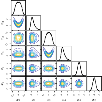
(a) Ground truth posterior for Multivariate Rosenbrock-Gaussian

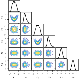
(b) svbmc result for Multivariate Rosenbrock-Gaussian

Figure S1: Multivariate Rosenbrock-Gaussian. Corner plot of example results associated with the $6D$ Multivariate Rosenbrock-Gaussian posterior with initial samples from cma-es.

Fig. S2 presents the corner plot of $q_{\phi}$ for the truncated dataset, used for demonstrating the active sampling capabilities of svbmc. Namely, the initial datapoints (in blue) are truncated for $x_{1}>0$, so that the algorithm has to actively sample points in the other half of the space (red points represent actively sampled points). The full graphs of the performance metrics are represented in Figs. S3 and S4.

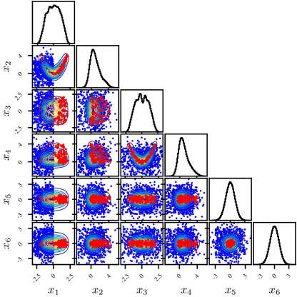
Figure S2: Multivariate Rosenbrock-Gaussian (truncated set). Example svbmc result for multivariate Rosenbrock-Gaussian with truncated initial samples. Blue points represent initial truncated cma-es samples (points with $x_{1}>0$ removed) and red points represent newly acquired samples with active sampling. Within a few dozen evaluations, svbmc is able to fully reconstruct the true target.

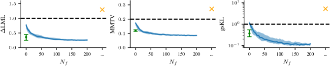
Figure S3: Performance on Rosenbrock-Gaussian posterior. $\Delta$LML loss (left), mmtv (center) and gsKL (right) as a function of number of post-processing target evaluations for the $6D$ Rosenbrock-Gaussian problem, with full initial set. The orange cross represents the Laplace approximation and the green dot the mcmc approximation, with its confidence interval.

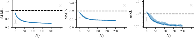
Figure S4: Performance on Rosenbrock-Gaussian posterior (truncated set). $\Delta$LML loss (left), mmtv (center) and gsKL (right) as a function of number of post-processing target evaluations for the $6D$ Rosenbrock-Gaussian problem, with truncated initial set. The cross represents the Laplace approximation and the dot the mcmc approximation, with its confidence interval. We copied the results from the standard initial set (light grey), as we only truncated the initial set to test the active learning ability of svbmc.

E.2.2 Two-Moons bimodal posterior

This distribution is inspired by the two moons dataset, but defined by a single analytical expression in $D=2$:

$$f(\mathbf{x}) =-\frac{1}{2}\left(\frac{r-1/\sqrt{2}}{0.01}\right)^{2}+\log(\exp(\kappa x_{1}/r)/3+2\exp(-\kappa x_{1}/r)/3),\qquad\mathbf{x}=(x_{1},x_{2}),\ r=\|\mathbf{x}\|_{2},$$

which corresponds in the polar coordinate system to an angle following a von Mises distribution and a normal radius. This density is not defined for $\mathbf{x}=0$, but remains defined for almost all $\mathbf{x}$ w.r.t. Lebesgue measure. We present in Fig. S5 the ground truth from extensive mcmc sampling (Fig. 5(a)), and example outputs from different algorithms:

• samples from the initial short mcmc runs, with no further post-processing (Fig. 5(b)), which exhibit failure of the algorithm to find the correct weights of the modes;

• the Laplace approximation from numerical differentiation (Fig. 5(c)), which fails to capture one of the modes;

• the svbmc variational posterior initialized from short mcmc runs (Fig. 5(d)), which perfectly reproduces the target.

(a) Ground truth Two-Moons bimodal posterior

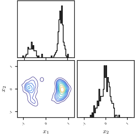
(b) Initial samples from short mcmc runs

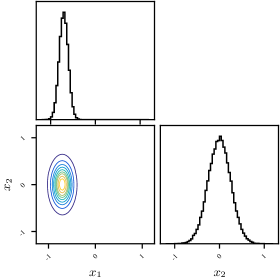
(c) Laplace approximation

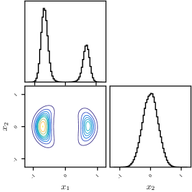
(d) svbmc result for Two-Moons bimodal posterior

Figure S5: Two-Moons bimodal posterior visualization. Example results from different algorithms.

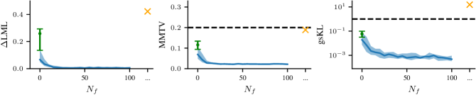
Figure S6: Performance on the Two-Moons bimodal posterior. $\Delta$LML loss (left), mmtv (center) and gsKL (right) as a function of number of post-processing target evaluations for the Two-Moons bimodal problem. The cross represents the Laplace approximation and the dot the mcmc approximation, with its confidence interval.

E.2.3 Lotka-Volterra model

The Lotka-Volterra differential equation system is a famous example of differential equations. It represents the joint evolution of two populations in the same space, predators and preys [Gilpin, 1973]. The equation writes:

$$\left\{\begin{matrix}\frac{\mathrm{d}u}{\mathrm{d}t}(t)=\alpha u(t)-\beta u(t)v(t)\\ \frac{\mathrm{d}v}{\mathrm{d}t}(t)=-\gamma v(t)+\delta u(t)v(t)\end{matrix}\right.,\quad u(0)=u_{0},v(0)=v_{0}$$

where $\alpha$ represents the birth rate of preys, $\beta$ the rate at which predators kill preys, $\gamma$ the death rate of predators, and $\delta$ the growth rate of predators. The dataset we use in our experiments comes from Howard [2009], with 20 yearly observation of $u$ and $v$. The likelihood is tractable if we are only interested in $u(t_{i})$ for a finite set of $t_{i}$.

Following [Carpenter, 2018], we assume noisy observations of $u$ and $v$ at times $t_{1},\dots,t_{T}$, with a LogNormal noise with intensity $\sigma_{u}$ and $\sigma_{v}$ respectively. In total the parameters of interest are $\alpha$, $\beta$, $\gamma$ and $\delta$, the evolution parameters; $\sigma_{u}$ and $\sigma_{v}$, the noise parameters; and $u_{0}$ and $v_{0}$ the initial values ($D=8$). The priors of the model are:

$$\alpha,\,\gamma \sim\mathcal{N}(1,0.5);$$ (S23)

$$\beta,\,\delta \sim\mathcal{N}(0.05,0.05);$$ (S24)

$$\sigma_{u},\,\sigma_{v} \sim\text{LogNormal}(-1,1)$$ (S25)

$$u_{0},\,v_{0} \sim\text{LogNormal}(\log(10),1)$$ (S26)

For this problem, we consider two different initialization sets for svbmc, one from multiple cma-es optimization runs, and one with initialization from multiple short mcmc runs for a total of 12k evaluations. For the mcmc initialization, we set $\eta_{\text{trim}}=20D$.

When multiple mcmc runs are available, the Bayesian stacking method from Yao et al. [2022] can be applied for post-processing the mcmc samples. One may think that stacking all the log-density evaluations produced throughout the run of the mcmc algorithm (slice sampling), instead of just the mcmc samples themselves, would give better results – since the number of evaluations is much larger than number of samples. However, running the Bayesian stacking method on log-density evaluations violates its underlying assumption that (approximate) posterior draws of parameters should be used. We also verified in practice that the Bayesian stacking method does not work well with cma-es evaluations and gives worse results in terms of metrics. For these reasons, for Bayesian stacking we only report the metrics obtained with mcmc samples.

The ground truth posterior is presented in Fig. 7(a), below which we show example variational posteriors obtained by svbmc using the two different initial datasets in Figs. 7(b) and 7(c). The performance metrics are presented in Figs. S9 and S8.

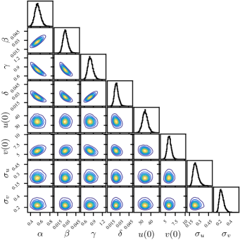
(a) Ground truth posterior for Lotka-Volterra model.

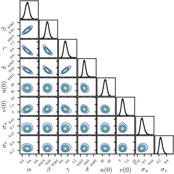
(b) svbmc result for Lotka-Volterra model with cma-es initial samples

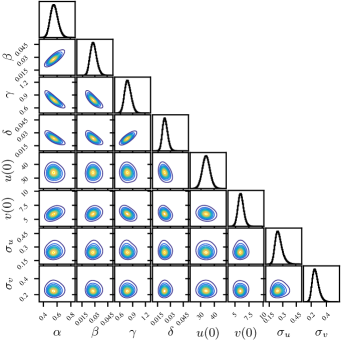
(c) svbmc result for Lotka-Volterra model with initial samples from short mcmc runs

Figure S7: Lotka-Volterra model posterior visualization.

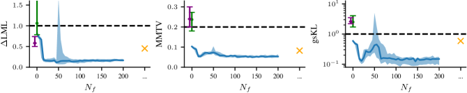
Figure S8: Performance on Lotka-Volterra model (mcmc initial samples). $\Delta$LML loss (left), mmtv (center) and gsKL (right) as a function of number of post-processing target evaluations for the Lotka-Volterra problem, with initial samples from short mcmc runs. The orange cross represents the Laplace approximation, the green dot the mcmc approximation and the purple diamond the Bayesian stacking method from Yao et al. [2022], with their confidence intervals.

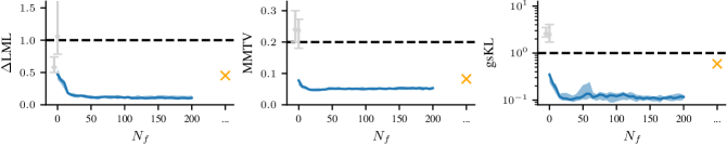
Figure S9: Performance on the Lotka-Volterra model (cma-es initial samples). $\Delta$LML loss (left), mmtv (center) and gsKL (right) as a function of number of post-processing target evaluations for the Lotka-Volterra problem, with the initial set from cma-es. The cross represents the Laplace approximation, the dot the mcmc approximation and the diamond the Bayesian stacking method from Yao et al. [2022], with their confidence intervals. Light grey results are copied from Fig. S8 since the corresponding methods are not applicable with the initial set from cma-es.

E.2.4 Bayesian timing model

We evaluate the svbmc algorithm with a popular model of Bayesian time perception [Jazayeri and Shadlen, 2010, Acerbi et al., 2012, Acerbi, 2020]. In each trial of a sensorimotor timing task, human subjects had to reproduce the time interval $\tau$ between a click and a flash, with $\tau\sim\text{Uniform}$[0.6, 0.975] s [Acerbi et al., 2012]. We assume subjects had only access to a noisy sensory measurement $t_{\text{s}}\sim\mathcal{N}\left(\tau,w_{\text{s}}^{2}\tau^{2}\right)$, and their reproduced time $t_{\text{m}}$ was affected by motor noise, $t_{\text{m}}\sim\mathcal{N}\left(\tau_{\star},w_{m}^{2}\tau_{\star}^{2}\right)$, where $w_{\text{s}}$ and $w_{\text{m}}$ are Weber’s fractions. We assume subjects estimated $\tau_{\star}$ by combining their sensory likelihood with an approximate Gaussian prior over time intervals, $\mathcal{N}\left({\tau};{\mu_{\text{p}}},{\sigma^{2}_{\text{p}}}\right)$, and took the mean of the resulting Bayesian posterior. For each trial we also consider a probability $\lambda$ of a ‘lapse’ (e.g., a misclick) producing a response $t_{\text{m}}\sim\text{Uniform}$[0, 2] s. Model parameters are $\bm{\theta}=(w_{\text{s}},w_{\text{m}},\mu_{\text{p}},\sigma_{\text{p}},\lambda)$, so $D=5$.

For this model, we use either exact evaluations or noisy evaluations of the log target density, with $\sigma_{\text{obs}}=5$. We calculated that the latter would correspond to noisy estimation of the log-likelihood using inverse binomial sampling with $N_{\text{rep}}\approx 100$ repeats [van Opheusden et al., 2020]. For the noisy-target case, for svbmc we used up to $N_{f}=900$ evaluations and $n_{\text{active}}=25$ active samples per iteration, as each log density evaluation carries less information. For the noiseless case, we kept the same values as other problems ($N_{f}=200$ and $n_{\text{active}}=5$). Note that the other considered methods (Laplace approximation, mcmc and Bayesian stacking) are unable to easily handle noisy evaluations of the log-density.

The initial samples for svbmc come from multiple optimization runs with cma-es (exact or stochastic). In the case of exact evaluations, we also run mcmc with the same or slightly bigger budget of function evaluations as cma-es for getting the samples. As discussed in Section E.2.3, the Bayesian stacking method is applied on these mcmc samples for post-processing and comparison.

In Fig. S10, we present a comparison of the ground truth posterior (Fig. 10(a)) and the svbmc variational posterior in the cases of exact evaluations (Fig. 10(b)) and noisy evaluations (Fig. 10(c)). The results in the case of noisy observations are quite similar to the noiseless case, indicating robustness of our method. The evolution of performance metrics is presented in Figs. S11 and S12.

(a) Ground truth posterior for Bayesian timing model

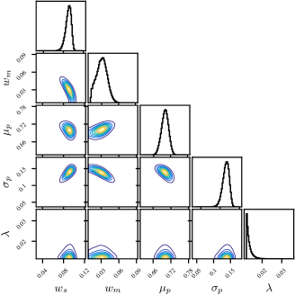
(b) svbmc result for timing model with exact evaluations

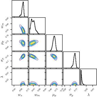
(c) svbmc result for noisy evaluations with $\sigma_{\text{obs}}=5$

Figure S10: Bayesian timing model posterior visualization. The initial samples for svbmc are from cma-es.

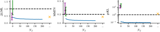
Figure S11: Performance on the Bayesian timing posterior (exact evaluations). $\Delta$LML loss (left), MMTV (center) and gsKL (right) as a function of number of post-processing target evaluations for the Bayesian timing problem, with noiseless evaluations of the target. The orange cross represents the Laplace approximation, the green dot the mcmc approximation and the purple diamond the Bayesian stacking method from Yao et al. [2022], with their confidence intervals.

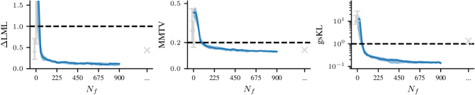
Figure S12: Performance on the Bayesian timing posterior (noisy evaluations). $\Delta$LML loss (left), MMTV (center) and gsKL (right) as a function of number of post-processing target evaluations for the Bayesian timing problem, with noisy evaluations of the target ($\sigma_{\text{obs}}=5$). The cross represents the Laplace approximation, the dot the mcmc approximation and the diamond the Bayesian stacking method from Yao et al. [2022], with their confidence intervals. We copied the light grey results from Fig. S11 purely for reference, as all these other algorithms do not work in the noisy case.

E.3 Ablation study of noise shaping

Noise shaping guides placement of inducing points in regions with higher log-densities and downweights observations that are with low log-densities. It helps sparse GP make better approximations in regions of interest with limited number of inducing points. Noise shaping is in practice needed, as running svbmc without it empirically decreases performance and could sometimes lead to catastrophic failures. We demonstrate the effect of noise shaping on the Lotka-Volterra model with 12k initial samples from short mcmc runs. As shown in Fig. S13, without noise shaping, the algorithm consistently fails to solve the problem, mostly due to a bad allocation of inducing points and training of the underlying sparse GP.

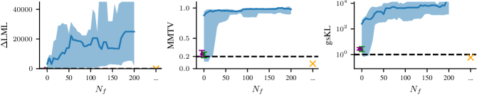
Figure S13: Ablation study: performance on the Lotka-Volterra posterior (12k mcmc initial samples) without noise shaping. $\Delta$LML loss (left), MMTV (center) and gsKL (right) as a function of number of post-processing target evaluations for the Lotka-Volterra problem. The orange cross represents the Laplace approximation, the green dot the mcmc approximation and the purple diamond the Bayesian stacking method, with their confidence intervals. Without noise shaping favoring regions of high-density in the sparse GP representation, the sparse GP is unable to adequately model the underlying target and svbmc systematically fails (compare with the performance in Fig. S8, which uses noise shaping).

E.4 Ablation study of active sampling

We introduced svbmc with a post-processing stage of active sampling, but one could wonder whether this stage is actually needed. The behavior of svbmc without active sampling (i.e., by simply fitting a sparse GP and variational posterior to the initial set) can be examined by looking at the performance curves of svbmc (Figs. S3, S4, S6, S9, S8, S11, S12), where the performance at $N_{f}=0$ corresponds to the starting svbmc with no additional target evaluations. We see that for simple problems (e.g., two moons, Fig. S6), active sampling only produces a small improvement. However, for complex, realistic problems (e.g., Bayesian timing model with noisy evaluations, Fig. S12) active sampling is essential to achieve a good solution.

References

- Acerbi [2018] Luigi Acerbi. Variational Bayesian Monte Carlo. Advances in Neural Information Processing Systems, 31:8222–8232, 2018.
- Acerbi [2019] Luigi Acerbi. An exploration of acquisition and mean functions in Variational Bayesian Monte Carlo. Proceedings of The 1st Symposium on Advances in Approximate Bayesian Inference (PMLR), 96:1–10, 2019.
- Acerbi [2020] Luigi Acerbi. Variational Bayesian Monte Carlo with noisy likelihoods. Advances in Neural Information Processing Systems, 33:8211–8222, 2020.
- Acerbi and Ma [2017] Luigi Acerbi and Wei Ji Ma. Practical Bayesian optimization for model fitting with Bayesian adaptive direct search. Advances in Neural Information Processing Systems, 30:1834–1844, 2017.
- Acerbi et al. [2012] Luigi Acerbi, Daniel M Wolpert, and Sethu Vijayakumar. Internal representations of temporal statistics and feedback calibrate motor-sensory interval timing. PLoS Computational Biology, 8(11):e1002771, 2012.
- Acerbi et al. [2018] Luigi Acerbi, Kalpana Dokka, Dora E Angelaki, and Wei Ji Ma. Bayesian comparison of explicit and implicit causal inference strategies in multisensory heading perception. PLoS Computational Biology, 14(7):e1006110, 2018.
- Bishop [2006] Christopher M Bishop. Pattern Recognition and Machine Learning. Springer, 2006.
- Bui and Turner [2014] Thang Bui and Richard Turner. On the paper: Variational learning of inducing variables in Sparse Gaussian Processes (Titsias, 2009). http://mlg.eng.cam.ac.uk/thang/docs/talks/rcc_vargp.pdf, 2014. Accessed: 2022-10-19.
- Burt et al. [2020] David R. Burt, Carl Edward Rasmussen, and Mark van der Wilk. Convergence of sparse variational inference in Gaussian processes regression. Journal of Machine Learning Research, 21(131):1–63, 2020.
- Carpenter [2018] Bob Carpenter. Predator-Prey Population Dynamics: the Lotka-Volterra model in Stan. https://mc-stan.org/users/documentation/case-studies/lotka-volterra-predator-prey.html, 2018.
- Carpenter et al. [2016] Bob Carpenter, Andrew Gelman, Matt Hoffman, Daniel Lee, Ben Goodrich, Michael Betancourt, Michael A Brubaker, Jiqiang Guo, Peter Li, and Allen Riddell. Stan: A probabilistic programming language. Journal of Statistical Software, 20, 2016.
- Carpenter et al. [2017] Bob Carpenter, Andrew Gelman, Matthew D Hoffman, Daniel Lee, Ben Goodrich, Michael Betancourt, Marcus Brubaker, Jiqiang Guo, Peter Li, and Allen Riddell. Stan: A probabilistic programming language. Journal of Statistical Software, 76(1), 2017.
- Chai and Garnett [2019] Henry R Chai and Roman Garnett. Improving quadrature for constrained integrands. In The 22nd International Conference on Artificial Intelligence and Statistics, pages 2751–2759. PMLR, 2019.
- Che et al. [2021] Yifeng Che, Xu Wu, Giovanni Pastore, Wei Li, and Koroush Shirvan. Application of Kriging and Variational Bayesian Monte Carlo method for improved prediction of doped UO2 fission gas release. Annals of Nuclear Energy, 153:108046, 2021. ISSN 0306-4549.
- Chen et al. [2018] Laming Chen, Guoxin Zhang, and Eric Zhou. Fast greedy map inference for determinantal point process to improve recommendation diversity. Advances in Neural Information Processing Systems, 31, 2018.
- Cheng and Boots [2016] Ching-An Cheng and Byron Boots. Incremental variational sparse Gaussian process regression. Advances in Neural Information Processing Systems, 29, 2016.
- De Souza et al. [2022] Daniel A De Souza, Diego Mesquita, Samuel Kaski, and Luigi Acerbi. Parallel MCMC without embarrassing failures. International Conference on Artificial Intelligence and Statistics, pages 1786–1804, 2022.
- Demetriades et al. [2022] Marios Demetriades, Marko Zivanovic, Myrianthi Hadjicharalambous, Eleftherios Ioannou, Biljana Ljujic, Ksenija Vucicevic, Zeljko Ivosevic, Aleksandar Dagovic, Nevena Milivojevic, Odysseas Kokkinos, et al. Interrogating and quantifying in vitro cancer drug pharmacodynamics via agent-based and Bayesian Monte Carlo modelling. Pharmaceutics, 14(4):749, 2022.
- Galy-Fajou and Opper [2021] Théo Galy-Fajou and Manfred Opper. Adaptive inducing points selection for Gaussian processes. arXiv preprint arXiv:2107.10066, 2021.
- Gelman et al. [2013] Andrew Gelman, John B Carlin, Hal S Stern, David B Dunson, Aki Vehtari, and Donald B Rubin. Bayesian Data Analysis (3rd edition). CRC Press, 2013.
- Gelman et al. [2020] Andrew Gelman, Aki Vehtari, Daniel Simpson, Charles C Margossian, Bob Carpenter, Yuling Yao, Lauren Kennedy, Jonah Gabry, Paul-Christian Bürkner, and Martin Modrák. Bayesian workflow. arXiv preprint arXiv:2011.01808, 2020.
- Geyer [1994] Charles J Geyer. Estimating normalizing constants and reweighting mixtures. (Technical report). 1994.
- Ghahramani [2015] Zoubin Ghahramani. Probabilistic machine learning and artificial intelligence. Nature, 521(7553):452–459, 2015.
- Ghahramani and Rasmussen [2002a] Zoubin Ghahramani and Carl Rasmussen. Bayesian Monte Carlo. In S. Becker, S. Thrun, and K. Obermayer, editors, Advances in Neural Information Processing Systems, volume 15. MIT Press, 2002a.
- Ghahramani and Rasmussen [2002b] Zoubin Ghahramani and Carl Rasmussen. Bayesian Monte Carlo. Advances in neural information processing systems, 15, 2002b.
- Gilpin [1973] Michael E. Gilpin. Do hares eat lynx? The American Naturalist, 107(957):727–730, 1973. ISSN 00030147, 15375323.
- Gunter et al. [2014] Tom Gunter, Michael A Osborne, Roman Garnett, Philipp Hennig, and Stephen J Roberts. Sampling for inference in probabilistic models with fast Bayesian quadrature. Advances in Neural Information Processing Systems, 27:2789–2797, 2014.
- Hansen et al. [2003] Nikolaus Hansen, Sibylle D Müller, and Petros Koumoutsakos. Reducing the time complexity of the derandomized evolution strategy with covariance matrix adaptation (CMA-ES). Evolutionary Computation, 11(1):1–18, 2003.
- Hansen et al. [2009] Nikolaus Hansen, André SP Niederberger, Lino Guzzella, and Petros Koumoutsakos. A method for handling uncertainty in evolutionary optimization with an application to feedback control of combustion. IEEE Transactions on Evolutionary Computation, 13(1):180–197, 2009.
- Hensman et al. [2013] James Hensman, Nicolò Fusi, and Neil D. Lawrence. Gaussian processes for big data. In Ann Nicholson and Padhraic Smyth, editors, Uncertainty in Artificial Intelligence, volume 29. AUAI Press, 2013.
- Hensman et al. [2015] James Hensman, Alexander Matthews, and Zoubin Ghahramani. Scalable variational Gaussian process classification. In Artificial Intelligence and Statistics, pages 351–360. PMLR, 2015.
- Howard [2009] Peter Howard. Modeling basics. Lecture Notes for Math, 442, 2009.
- Järvenpää et al. [2019] Marko Järvenpää, Michael U Gutmann, Arijus Pleska, Aki Vehtari, Pekka Marttinen, et al. Efficient acquisition rules for model-based approximate Bayesian computation. Bayesian Analysis, 14(2):595–622, 2019.
- Järvenpää et al. [2021] Marko Järvenpää, Michael U Gutmann, Aki Vehtari, and Pekka Marttinen. Parallel Gaussian process surrogate Bayesian inference with noisy likelihood evaluations. Bayesian Analysis, 16(1):147–178, 2021.
- Jazayeri and Shadlen [2010] Mehrdad Jazayeri and Michael N Shadlen. Temporal context calibrates interval timing. Nature Neuroscience, 13(8):1020–1026, 2010.
- Jones et al. [1998] Donald R Jones, Matthias Schonlau, and William J Welch. Efficient global optimization of expensive black-box functions. Journal of Global Optimization, 13(4):455–492, 1998.
- Jordan et al. [1999] Michael I Jordan, Zoubin Ghahramani, Tommi S Jaakkola, and Lawrence K Saul. An introduction to variational methods for graphical models. Machine Learning, 37(2):183–233, 1999.
- Kanagawa and Hennig [2019] Motonobu Kanagawa and Philipp Hennig. Convergence Guarantees for Adaptive Bayesian Quadrature methods. Advances in Neural Information Processing Systems, 32:6234–6245, 2019.
- Kanagawa et al. [2018] Motonobu Kanagawa, Philipp Hennig, Dino Sejdinovic, and Bharath K Sriperumbudur. Gaussian processes and kernel methods: A review on connections and equivalences. arXiv preprint arXiv:1807.02582, 2018.
- Kandasamy et al. [2015] Kirthevasan Kandasamy, Jeff Schneider, and Barnabás Póczos. Bayesian active learning for posterior estimation. Twenty-Fourth International Joint Conference on Artificial Intelligence, 2015.
- Kingma and Ba [2014] Diederik P Kingma and Jimmy Ba. Adam: A method for stochastic optimization. Proceedings of the 3rd International Conference on Learning Representations, 2014.
- Kingma and Welling [2013] Diederik P Kingma and Max Welling. Auto-encoding variational Bayes. Proceedings of the 2nd International Conference on Learning Representations, 2013.
- Maddox et al. [2021] Wesley J Maddox, Samuel Stanton, and Andrew G Wilson. Conditioning sparse variational Gaussian processes for online decision-making. In M. Ranzato, A. Beygelzimer, Y. Dauphin, P.S. Liang, and J. Wortman Vaughan, editors, Advances in Neural Information Processing Systems, volume 34, pages 6365–6379. Curran Associates, Inc., 2021.
- Matthews et al. [2017] Alexander G. de G. Matthews, Mark van der Wilk, Tom Nickson, Keisuke. Fujii, Alexis Boukouvalas, Pablo León-Villagrá, Zoubin Ghahramani, and James Hensman. GPflow: A Gaussian process library using TensorFlow. Journal of Machine Learning Research, 18(40):1–6, apr 2017.
- McIntire et al. [2016] Mitchell McIntire, Daniel Ratner, and Stefano Ermon. Sparse Gaussian Processes for Bayesian Optimization. In UAI, 2016.
- Miller et al. [2017] Andrew C Miller, Nicholas Foti, and Ryan P Adams. Variational boosting: Iteratively refining posterior approximations. Proceedings of the 34th International Conference on Machine Learning, 70:2420–2429, 2017.
- Neal [2003] Radford M Neal. Slice sampling. Annals of Statistics, 31(3):705–741, 2003.
- Neiswanger et al. [2013] Willie Neiswanger, Chong Wang, and Eric Xing. Asymptotically exact, embarrassingly parallel MCMC. arXiv preprint arXiv:1311.4780, 2013.
- Nemeth and Sherlock [2018] Christopher Nemeth and Chris Sherlock. Merging MCMC subposteriors through Gaussian-process approximations. Bayesian Analysis, 13(2):507–530, 2018.
- O’Hagan [1991] Anthony O’Hagan. Bayes–Hermite quadrature. Journal of Statistical Planning and Inference, 29(3):245–260, 1991.
- Osborne et al. [2012] Michael Osborne, David K Duvenaud, Roman Garnett, Carl E Rasmussen, Stephen J Roberts, and Zoubin Ghahramani. Active learning of model evidence using Bayesian quadrature. Advances in Neural Information Processing Systems, 25:46–54, 2012.
- Ranganath et al. [2014] Rajesh Ranganath, Sean Gerrish, and David Blei. Black box variational inference. In Artificial Intelligence and Statistics, pages 814–822. PMLR, 2014.
- Rasmussen and Williams [2006] C. Rasmussen and C. K. I. Williams. Gaussian Processes for Machine Learning. MIT Press, 2006.
- Rasmussen [2003] Carl Edward Rasmussen. Gaussian processes to speed up hybrid Monte Carlo for expensive Bayesian integrals. Bayesian Statistics, 7:651–659, 2003.
- Rasmussen and Williams [2005] Carl Edward Rasmussen and Christopher K. I. Williams. Gaussian Processes for Machine Learning. The MIT Press, 2005.
- Robert et al. [2009] Christian P Robert, Darren Wraith, Paul M Goggans, and Chun-Yong Chan. Computational methods for bayesian model choice. In AIP Conference Proceedings, volume 1193, pages 251–262. AIP, 2009.
- Robert et al. [2007] Christian P Robert et al. The Bayesian choice: from decision-theoretic foundations to computational implementation, volume 2. Springer, 2007.
- Seeger [2004] Matthias W. Seeger. Low rank updates for the cholesky decomposition. 2004.
- Snelson and Ghahramani [2005] Edward Snelson and Zoubin Ghahramani. Sparse gaussian processes using pseudo-inputs. In Y. Weiss, B. Schölkopf, and J. Platt, editors, Advances in Neural Information Processing Systems, volume 18. MIT Press, 2005.
- Snelson and Ghahramani [2006] Edward Snelson and Zoubin Ghahramani. Sparse Gaussian processes using pseudo-inputs. Advances in Neural Information Processing Systems, 18:1259–1266, 2006.
- Snoek et al. [2012] Jasper Snoek, Hugo Larochelle, and Ryan P Adams. Practical Bayesian optimization of machine learning algorithms. Advances in Neural Information Processing Systems, 25:2951–2959, 2012.
- Stine et al. [2020] Gabriel M Stine, Ariel Zylberberg, Jochen Ditterich, and Michael N Shadlen. Differentiating between integration and non-integration strategies in perceptual decision making. Elife, 9:e55365, 2020.
- Sweeting [1986] T. J. Sweeting. On a Converse to Scheffe’s Theorem. The Annals of Statistics, 14(3):1252 – 1256, 1986.
- Titsias [2009] Michalis Titsias. Variational learning of inducing variables in sparse Gaussian processes. In Artificial intelligence and statistics, pages 567–574. PMLR, 2009.
- Tsybakov [2003] Alexandre B Tsybakov. Introduction à l’estimation non paramétrique, volume 41. Springer Science & Business Media, 2003.
- van Opheusden et al. [2020] Bas van Opheusden, Luigi Acerbi, and Wei Ji Ma. Unbiased and efficient log-likelihood estimation with inverse binomial sampling. PLOS Computational Biology, 16(12):e1008483, 2020. doi: 10.1371/journal.pcbi.1008483.
- Wang and Li [2018] Hongqiao Wang and Jinglai Li. Adaptive Gaussian process approximation for Bayesian inference with expensive likelihood functions. Neural Computation, pages 1–23, 2018.
- Wilson and Adams [2013] Andrew Wilson and Ryan Adams. Gaussian process kernels for pattern discovery and extrapolation. In Proceedings of the 30th International Conference on Machine Learning, volume 28, pages 1067–1075. PMLR, 2013.
- Wood [2010] Simon N Wood. Statistical inference for noisy nonlinear ecological dynamic systems. Nature, 466(7310):1102–1104, 2010.
- Yao et al. [2022] Yuling Yao, Aki Vehtari, and Andrew Gelman. Stacking for non-mixing Bayesian computations: The curse and blessing of multimodal posteriors. Journal of Machine Learning Research, 23(79):1–45, 2022.