Fredholm integral equations for function approximation and the training of neural networks

Abstract.

We present a novel and mathematically transparent approach to function approximation and the training of large, high-dimensional neural networks, based on the approximate least-squares solution of associated Fredholm integral equations of the first kind by Ritz-Galerkin discretization, Tikhonov regularization and tensor-train methods. Practical application to supervised learning problems of regression and classification type confirm that the resulting algorithms are competitive with state-of-the-art neural network-based methods.

1. Introduction

Efficient and reliable methods for the training of neural networks are of fundamental importance for a multitude of applications and therefore a flourishing field of mathematical research. Stochastic gradient methods [1, 2] are known and further developed since the sixties. These methods mostly perform very well and therefore are often considered as methods of choice in the field. However, global convergence analysis is complicated and actual convergence might depend on proper parameter tuning [3]. Multilevel trust region methods [4, 5, 6] on the one hand aim at increasing efficiency by Newton-type linearization and on the other hand at increasing reliability by suitable step size control. Multilevel versions [7] are intended to additionally transfer the efficiency of multigrid methods for the minimization of energy functionals associated with elliptic partial differential equations to the minimization of loss functionals.

This paper is devoted to a novel and mathematically transparent approach to function approximation and the training of large and high-dimensional shallow neural networks with usual kernel functions $\psi$, training parameters $(\eta_{i},u_{i})_{i=1}^{N}$ with $\eta_{i}\in Q\subset\mathbb{R}^{s}$, $u_{i}\in\mathbb{R}$, $I=1,\dots,N$, and intentionally large $s$ and $N$. The starting point of our considerations is that such neural networks can be interpreted as Monte-Carlo approximations of integrals over $Q$, once the parameters $\eta_{i}$ are assumed to be equidistributed on $Q$ (see also [8]). Resulting Fredholm integral operators, now acting on parameter functions rather than parameter vectors, give rise to so-called Fredholm networks providing a novel approach to function approximation. Training of such Fredholm networks amounts to least-squares solution of linear Fredholm integral equations of the first kind for a parameter function $u\colon Q\to\mathbb{R}$, the continuous counterpart of the discrete parameter vector $(u_{i})_{i=1}^{N}$. Fredholm-trained parameters $(\eta_{i},u(\eta_{i}))_{i=1}^{N}$ of the original discrete neural network are then obtained by suitable sampling of $\eta_{i}\in Q$. A similar approach has been developed for kernel methods in supervised and semi-supervised learning [9, 10, 11] and applied to the covariance shift problem in transfer learning [12].

In general, the solution $u$ of the continuous Fredholm training problem is not available. After Ritz-Galerkin discretization with suitable ansatz space and Tikhonov regularization [13], the resulting, intentionally large, linear systems are approximately solved by tensor-train methods, such as alternating linear schemes [14, 15]. Approximately Fredholm-trained parameters $(\tilde{\eta}_{i},\tilde{u}(\tilde{\eta}_{i}))_{i=1}^{N}$ of the original neural network are finally obtained from the resulting approximation $\tilde{u}$ of $u$ and suitable sampling of $\tilde{\eta}_{i}\in Q$. While the numerical analysis of this approach is devoted to a forthcoming paper, the goal of this work is to confirm the practical potential of the Fredholm approach by numerical experiments and comparison with state-of-the-art neural network-based methods.

The paper is organized as follows. After describing the architecture of the neural networks in question together with the resulting discrete training problem in the next Section 2, we introduce Fredholm networks and Fredholm training problems as their continuous counterparts and briefly discuss ill-posedness in Section 3. Ritz-Galerkin discretization and Tikhonov regularization are presented in Section 4. Utilizing suitable factorizations of the kernel functions $\psi$ (as derived in the Appendix A), Section 5 is devoted to tensor-train methods for the iterative solution of the large linear systems associated with intentionally high-dimensional parameter domains $Q\subset\mathbb{R}^{s}$. In Section 6, we harvest the results on the training of Fredholm networks, briefly discuss Monte-Carlo sampling, and introduce a novel inductive importance sampling strategy. In the final Section 7, we apply our methods to three well-established test problems of regression and classification type with different computational complexity. In particular, we consider the UCI banknote authentication data set from [16], concrete compressive strength prediction [17, 18, 19, 20], and the well-known MNIST data set [21]. For all these problems, Fredholm networks and Fredholm-trained neural networks turn out to be highly competitive with state-of-the-art approaches without any problem-specific features or tuning. The efficiency of Fredholm-trained neural networks however seems to rely on a careful choice of sampling strategy: While straightforward quasi-Monte-Carlo sampling appears to work perfectly well for simple problems, more advanced strategies, such as inductive importance sampling, seem to be required in more complicated cases.

2. Large single layer neural networks

2.1. Architecture

We consider a parametrized single layer neural network of the form

(1) $$X\ni x\mapsto F_{N}(x,\zeta)=\frac{1}{N}\sum_{i=1}^{N}\psi(x,\eta_{i})u_{i}\in\mathbb{R}$$

defined on a compact hypercube $X\subset\mathbb{R}^{d}$, for simplicity, with intentionally large number of neurons $N\in\mathbb{N}$, a suitable kernel function $\psi:X\times Q\to\mathbb{R}$, and associated parameter vector

$$\zeta=(\zeta_{i})_{i=1}^{N},\quad\zeta_{i}=(\eta_{i},u_{i})\in Q\times\mathbb{R},$$

where $Q=Q_{1}\times\cdots\times Q_{s}\subset\mathbb{R}^{s}$.

Ridge kernel functions

(2) $$\psi(x,\eta)=\sigma(w\cdot x+b),\quad\eta=(w,b)\in Q\subset\mathbb{R}^{s},\;s=d+1,$$

are characterized by suitable activation functions $\sigma:\mathbb{R}\to\mathbb{R}$ and give rise to so-called single hidden layer perceptron models [22]. In the simplest case $\sigma\equiv\text{Id}$ and $b=0$, this definition reduces to the Euclidean scalar product $\psi(x,\eta)=x\cdot\eta$ with $\eta=w\in\mathbb{R}^{s}$ and $s=d$. More relevant choices for $\sigma$ include the (discontinuous) Heaviside function

(3) $$\sigma_{\infty}(z)=\left\{\begin{array}[]{ccl}0&\text{ if }z<0,\\ 1/2&\text{ if }z=0,\\ 1&\text{ if }z>0\\ \end{array}\right.$$

or suitable regularizations like the logistic activation function

(4) $$\sigma_{\kappa}(z)=\frac{\exp(\kappa z)}{1+\exp(\kappa z)}$$

with $\kappa>0$. Note that $\sigma_{\kappa}(z)\to\sigma_{\infty}(z)$ holds for $\kappa\to\infty$ and all $z\in\mathbb{R}$.

Radial kernel functions [23] are given by

(5) $$\psi(x,\eta)=\sigma(\lVert x-w\rVert),\quad\eta=w\in Q\subset\mathbb{R}^{s},\;s=d,$$

with some vector norm $\lVert\,\cdot\,\rVert$ on $\mathbb{R}^{d}$ and suitable activation functions $\sigma$. In the case of Gaussian activation functions

(6) $$\sigma(z)=\exp\left(-\frac{z^{2}}{2\kappa^{2}}\right)$$

and the Euclidean norm $\lVert\,\cdot\,\rVert=\lVert\,\cdot\,\rVert_{2}$, we have

(7) $$\psi(x,\eta)=\exp\left(-\frac{\lVert x-\eta\rVert_{2}^{2}}{2\kappa^{2}}\right)=\prod_{k=1}^{d}\exp\left(-\frac{(x_{k}-\eta_{k})^{2}}{2\kappa^{2}}\right).$$

2.2. Function data, loss functional, and training

Throughout the following $L^{2}(X,\pi)$ stands for the Hilbert space of $\pi$ measurable, quadratically integrable functions on $X$ with canonical scalar product $(\cdot,\cdot)_{\pi}$ and induced norm $\|\cdot\|_{\pi}$. We write $L^{2}(X)=L^{2}(X,\pi)$ and $(\cdot,\cdot)_{X}=(\cdot,\cdot)_{\pi}$, $\|\cdot\|_{X}=\|\cdot\|_{\pi}$, if $d\pi(x)=dx$ is the Lebesgue measure. Furthermore, $L^{2}(Q)$ stands for the Hilbert space of Lebesgue measurable, quadratically integrable functions on $Q$ with canonical scalar product $(\cdot,\cdot)$ and induced norm $\|\cdot\|$.

We aim at the approximation of a function $F:X\mapsto\mathbb{R}$ by parametrized ansatz functions $F_{N}(\cdot,\zeta)$ of the form (1). The parameters $\zeta$ are determined by minimizing the loss functional

(8) $$\mathcal{J}_{N}(\zeta)=\|F-F_{N}(\cdot,\zeta)\|_{\pi}^{2}=\int_{X}(F(x)-F_{N}(x,\zeta))^{2}\;d\pi(x)$$

where the measure $\pi$ is associated with the training data available. We will consider the following two cases of given

(9) $$\text{ a) function data}\;\;F\in L^{2}(X)\quad\text{ b) point data}\;\;((x_{j},F(x_{j})))_{j=1}^{M}\in(X\times\mathbb{R})^{M}\subset\mathbb{R}^{M(d+1)}.$$

The case a) of a given function $F$ is associated with the Lebesgue measure $d\pi(x)=dx$ while case b) of given point data corresponds to the point measure $d\pi(x)=d\mu(x)$,

(10) $$\mu=\frac{1}{M}\sum_{j=1}^{M}\delta_{x_{j}},\quad x_{1},\dots,x_{M}\in X.$$

Training of the neural network $F_{N}(\cdot,\zeta)$ amounts to the (approximate) solution of the following discrete, non-convex, large-scale minimization problem.

Problem 2.1.

Find $\zeta^{*}=(\zeta_{i}^{*})_{i=1}^{N},\;\zeta_{i}^{*}=(\eta^{*}_{i},u^{*}_{i})\in Q\times\mathbb{R}$, such that

(11) $$\mathcal{J}_{N}(\zeta^{*})\leq\mathcal{J}_{N}(\zeta)\qquad\forall\zeta=(\zeta_{i})_{i=1}^{N},\;\zeta_{i}=(\eta_{i},u_{i})\in Q\times\mathbb{R}.$$

Approximation properties of neural networks of the form (1) have quite a history (see, e.g., [24] or the overview of Pinkus  [22]). In particular, ridge kernels with any non-polynomial activation function $\sigma$ and unconstrained parameters $\zeta\in\mathbb{R}^{N(d+2)}$ provide uniform approximation of continuous functions $F$ on compact sets $X\subset\mathbb{R}^{d}$ [22, Theorem 3.1]. While similar results for constrained parameters $\zeta\in Q\times\mathbb{R}$ seem to be rare, the following proposition is a consequence of [25, Theorem 2.6].

Proposition 2.2.

For the ridge kernel (2) with logistic activation function (4), $Q$ containing the unit ball in $\mathbb{R}^{d+1}$, and any function $F\in C(X)$, we have

(12) $$\underset{\zeta\in(Q\times\mathbb{R})^{N}}{\inf}\;\underset{x\in X}{\max}\;|F(x)-F_{N}(x,\zeta)|\to 0\quad\text{for}\quad N\to\infty.$$

Hence, assuming existence of a solution $\zeta^{*}$ for all $N\in\mathbb{N}$, we have $\mathcal{J}_{N}(\zeta^{*})\to 0$ as $N\to\infty$ for $F\in L^{2}(X)$ in the case (9a) and $F\in C(X)$ in the case (9b), respectively.

3. Continuous approximations of discrete training problems

Following the ideas from [8, Section 1.2], we now introduce and investigate the asymptotic limit of $F_{N}(\cdot,\zeta)$ and of the corresponding Training Problem 2.1 for $N\to\infty$.

3.1. Asymptotic integral operators

Assume that $\psi(x,\cdot)\in L^{2}(Q)$ for each fixed $x\in X$. Let $\eta_{i}$, $i=1,...,N$, be independent, identically equidistributed random variables. Then, denoting $|Q|=\int_{Q}1\;dx$,

(13) $$\frac{1}{N}\sum_{i=1}^{N}\psi(x,\eta_{i})v(\eta_{i})\;\to\;\frac{1}{|Q|}\int_{Q}\psi(x,\eta)v(\eta)\;d\eta\quad\text{for}\quad N\to\infty$$

holds for all $v\in L^{2}(Q)$ and each fixed $x\in X$ by the strong law of large numbers.

This observation suggests to consider the Fredholm integral operator

(14) $$\mathcal{G}v=\frac{1}{|Q|}\int_{Q}\psi(\cdot,\eta)v(\eta)\;d\eta,\quad v\in L^{2}(Q),$$

Let us recall some well-known properties of $\mathcal{G}$, cf. [13, 26, 27].

Proposition 3.1.

Assume that

(15) $$\int_{X}\int_{Q}\psi(x,\eta)^{2}\;d\eta\;dx<\infty.$$

Then the integral operator

$$\mathcal{G}:L^{2}(Q)\to L^{2}(X)$$

is a compact, linear mapping.

Note that Proposition 3.1 provides compactness of $\mathcal{G}$, e.g., for the radial and ridge kernel functions mentioned in Section 2.1.

3.2. Fredholm integral equations

3.2.1. Function data

Let us first consider the case (9a) of a given function $F\in L^{2}(X)$. In the light of (13), we impose the additional constraints on the unknowns $\zeta_{i}=(\eta_{i},u_{i})$, $i=1,\dots,N$, of the Training Problem 2.1 that

(16) $$\eta_{i}\text{ are samples of i.i.~{}equidistributed random variables and }u_{i}=u(\eta_{i}),\quad i=1,\dots,N,$$

with some function $u\in L^{2}(Q)$. Then, for given function $F$, the asymptotic coincidence (13) of the discrete neural network $F_{N}(\cdot,((\eta_{i},u_{i})_{i=1}^{N})$ and the integral operator $\mathcal{G}u$ suggests to consider the loss functional

(17) $$\mathcal{J}(v)=\int_{X}(F(x)-\mathcal{G}v(x))^{2}\;dx.$$

and the following continuous quadratic approximation of the discrete non-convex Training Problem 2.1.

Problem 3.2.

Find $u\in L^{2}(Q)$ such that

(18) $$\mathcal{J}(u)\leq\mathcal{J}(v)\quad\forall v\in L^{2}(Q).$$

Observe that Problem 3.2 is just the least-squares formulation of the Fredholm integral equation of the first kind

(19) $$\mathcal{G}u=\frac{1}{|Q|}\int_{Q}\psi(\cdot,\eta)u(\eta)\;d\eta=F.$$

In particular, (18) can be equivalently rewritten as the normal equation

(20) $$\mathcal{G}^{*}\mathcal{G}u=\mathcal{G}^{*}F\quad\text{in}\quad L^{2}(Q)$$

utilizing the variational formulation of (18),

(21) $$(\mathcal{G}u,\mathcal{G}v)_{X}=(F,\mathcal{G}v)_{X}\qquad\forall v\in L^{2}(Q),$$

and the adjoint operator of $\mathcal{G}$,

$$L^{2}(X)\ni v\mapsto\mathcal{G}^{*}v=\frac{1}{|Q|}\int_{X}\psi(x,\cdot)v(x)\;dx\in L^{2}(Q).$$

This leads to the following well-known existence result (see, e.g., [13, Theorem 2.5]), where $R(\mathcal{G})$ and $N(\mathcal{G})$ stand for the range and null space of $\mathcal{G}$, respectively, $\oplus$ denotes the direct sum, and the superscript $\perp$ indicates the orthogonal complement in $L^{2}(X)$.

Proposition 3.3.

Assume that $F\in R(\mathcal{G})+R(\mathcal{G})^{\perp}\subset L^{2}(X)$. Then (19) has least-squares solutions $u^{\dagger}\oplus N(\mathcal{G})$, with $u^{\dagger}=\mathcal{G}^{\dagger}F$ being the unique minimal-norm least squares solution (best-approximate solution), and $\mathcal{G}^{\dagger}\colon R(\mathcal{G})\oplus R(\mathcal{G})^{\perp}\to N(\mathcal{G})^{\perp}\subset L^{2}(Q)$ denoting the generalised Moore-Penrose inverse of $\mathcal{G}$.

If $\mathcal{G}$ is compact, then $R(\mathcal{G})$ is closed or, equivalently, $\mathcal{G}^{\dagger}$ is bounded, if and only if $R(\mathcal{G})$ has finite dimension (see, e.g., [13, Proposition 2.7]). As a consequence, the integral equation (19) is ill-posed, even in the least-squares sense (18) for usual kernel functions such as the radial and ridge kernels presented in Section 2.1.

Proposition 3.4.

Assume that the kernel function $\psi$ is discriminatory in the sense that

(22) $$N(\mathcal{G}^{*})=\{0\}.$$

Then $R(\mathcal{G})$ is dense in $L^{2}(X)$ and therefore $\underset{u\in L^{2}(Q)}{\inf}{\mathcal{J}}(u)=0$ holds for all $F\in L^{2}(X)$.

For ridge kernels with Heaviside or logistic activation function, we obtain $v=0$, if $\mathcal{G}^{*}v(\eta)=0$ holds for all $\eta\in\mathbb{R}^{s}$ (and not only for all $\eta\in Q$) by [28, Lemma 1]. However, similar results for the present case of bounded parameters $\eta\in Q$ seem to be unknown.

Remark 3.5.

In order to relax the constraints (16) on the parameters $\zeta$ that provide an asymptotic limit of $F_{N}(\cdot,\zeta)$ of the form (13), one might assume that the parameters $\zeta_{i}=(\eta_{i},u_{i})$ are independent random variables that are identically distributed with respect to some unknown probability measure $\nu\in\mathbb{P}(Q\times\mathbb{R})$. Then, the law of large numbers implies

$$\frac{1}{N}\sum_{i=1}^{N}\psi(x,\eta_{i})u_{i}\longrightarrow\int_{Q\times\mathbb{R}}\psi(x,\eta)u\;d\nu(\eta,u)\quad\text{for }N\longrightarrow\infty$$

in analogy to (13). Replacing $F_{N}(x,\zeta)$ in the loss functional $\mathcal{J}_{N}$ by the integral operator

$$\mathbb{P}(Q\times\mathbb{R})\ni\nu\mapsto\int_{Q\times\mathbb{R}}\psi(\cdot,\eta)u\;d\nu(\eta,u)\in\mathbb{R}$$

the resulting training problem for the parameter measure $\nu$ amounts to the least squares formulation of the problem to find $\nu\in\mathbb{P}(Q\times\mathbb{R})$ such that

(23) $$\int_{Q\times\mathbb{R}}\psi(\cdot,\eta)u\;d\nu(\eta,u)=F.$$

The analysis and numerical analysis of such Fredholm integral equations on measures is the subject of ongoing research.

3.2.2. Point data

In the case (9b) of given point values of $F$, we replace the corresponding point values of $F_{N}$ in (8) by the point values of the limiting integral operator $\mathcal{G}$ to obtain the approximation $J$,

$$J(v)=\frac{1}{M}\sum_{j=1}^{M}(F(x_{j})-\mathcal{G}v(x_{j}))^{2},$$

of the discrete loss functional $\mathcal{J}_{N}$ and the following quadratic approximation of the Training Problem 2.1.

Problem 3.6.

Find $u\in L^{2}(Q)$ such that

(24) $$J(u)\leq J(v)\quad\forall v\in L^{2}(Q).$$

Problem 3.6 is the least-squares formulation of the interpolation problem to find $u\in L^{2}(Q)$ such that

$$\mathcal{G}_{M}u=F_{M}$$

with $F_{M}=(F(x_{j}))_{j=1}^{M}\in\mathbb{R}^{M}$ and $\mathcal{G}_{M}\colon L^{2}(Q)\to\mathbb{R}^{M}$ defined by $\mathcal{G}_{M}v=(\mathcal{G}v(x_{i}))_{i=1}^{M}\in\mathbb{R}^{M}$. In analogy to (20), Problem 3.6 can be equivalently reformulated as a linear normal equation $\mathcal{G}_{M}^{*}\mathcal{G}_{M}u=\mathcal{G}_{M}^{*}F_{M}$ in $L^{2}(Q)$ utilizing the variational formulation

(25) $$\sum_{j=1}^{M}(\mathcal{G}u)(x_{j})(\mathcal{G}v)(x_{j})=\sum_{j=1}^{M}F(x_{j})(\mathcal{G}v)(x_{j})\qquad\forall v\in L^{2}(Q),$$

of Problem 3.6 with the adjoint operator $\mathcal{G}_{M}^{*}$ of $\mathcal{G}_{M}$ given by

$$\mathbb{R}^{M}\ni v=(v_{j})_{j=1}^{M}\mapsto\mathcal{G}_{M}^{*}v=\frac{1}{|Q|}\sum_{j=1}^{M}\psi(x_{j},\cdot)v_{j}\in L^{2}(Q).$$

Observe that $R(\mathcal{G}_{M})$ is now finite-dimensional and thus closed. Hence, existence of a best-approximate solution $u=\mathcal{G}_{M}^{\dagger}$ of Problem 3.6 for any point data $(x_{i},F(x_{i}))$, $i=1,\dots,M$, follows from $R(\mathcal{G}_{M})\oplus R(\mathcal{G}_{M})^{\perp}=\mathbb{R}^{M}$ and the general Theorem 2.5 in [13]. As a consequence, the Moore-Penrose inverse $\mathcal{G}_{M}^{\dagger}$ is now bounded. However, its norm is expected to increase with increasing $M$.

Remark 3.7.

Assuming $N(\mathcal{G}_{N}^{*})=\{0\}$, we obtain $J(u)=0$ in analogy to Proposition 3.4.

3.3. Fredholm networks

The asymptotic coincidence with discrete neural networks $F_{N}(\cdot,\eta)$ suggests to consider their continuous counterpart

(26) $$\mathcal{G}v=\frac{1}{|Q|}\int_{Q}\psi(\cdot,\eta)v(\eta)\;d\eta$$

with parameter function $v\in L^{2}(Q)$ directly for approximation. Observe that the continuous Training Problems 3.2 (function data) or 3.6 (point data) associated with such Fredholm networks are linear, in contrast to the original discrete Problem 2.1. However, linearity comes with the price of infinitely many unknown parameter function values. This suggests suitable discretizations of the continuous Training Problem 3.2 or 3.6 providing computable approximations of the corresponding Fredholm networks. For example, the integral operator $\mathcal{G}$ has been replaced by a suitable Riemann sum in [9, 10, 11].

4. Ritz-Galerkin discretization and regularization

4.1. Variational formulation

Let $L\subset L^{2}(Q)$ denote a closed subspace. Then the corresponding Ritz-Galerkin discretization of the Fredholm Training Problems 3.2 and 3.6 reads as follows.

Problem 4.1.

Find $u_{L}\in L$ such that

(27) $$(\mathcal{G}u_{L},\mathcal{G}v)_{\pi}=(F,\mathcal{G}v)_{\pi}\qquad\forall v\in L,$$

with $\pi$ still denoting the Lebesgue or point measure.

Again, existence of a best-approximate solution $u_{L}$ follows from Theorem 2.5 in [13], and asymptotic ill-conditioning is expected to be inherited from the continuous case.

4.2. Algebraic formulation

Let the ansatz space $L=L_{n}$ have finite dimension $n$ and let $\varphi_{1},\dots,\varphi_{n}$ be a basis of $L_{n}$. Then any $v\in L_{n}$ can be identified with the coefficient vector $V=(V_{i})_{i=1}^{n}\in\mathbb{R}^{n}$ of its unique basis representation

(28) $$v=\sum_{i=1}^{n}V_{i}\varphi_{i}\in L_{n}.$$

Example 4.2.

Let $Q=\bigcup_{i=1}^{n}q_{i}$ be a decomposition of $Q$ into disjoint rectangles $q_{i}$ with maximal edge length $h$. Then

$$\varphi_{i}(\eta)=\left\{\begin{array}[]{cc}|q_{i}|^{-1/2}&\text{if }\eta\in q_{i}\\ 0&\text{otherwise}\end{array}\right.$$

is an orthonormal basis of the subspace $L_{n}\subset L^{2}(Q)$ of piecewise constant functions on $q_{i}$, and the coefficients $V_{i}$ of $v\in L_{n}$ agree with its scaled values on $q_{i}$, $i=1,\dots,n$.

Introducing the semi-discrete, linear operators

(29) $$\begin{array}[]{lclrll}G&=&(\mathcal{G}\varphi_{1},\dots,\mathcal{G}\varphi_{n})&\in L^{2}(X,\pi)\times\mathbb{R}^{n}\colon&\mathbb{R}^{n}\to L^{2}(X,\pi),\\ G^{*}&=&((\mathcal{G}\varphi_{i},\cdot)_{\pi})_{i=1}^{n}&\in\mathbb{R}^{n}\times L^{2}(X,\pi)\colon&L^{2}(X,\pi)\to\mathbb{R}^{n}\end{array}$$

we have $\mathcal{G}u_{L}=GU$ with $u_{L}=\sum_{i=1}^{n}U_{i}\varphi_{i}$ and $U=(U_{i})_{i=1}^{n}\in\mathbb{R}^{n}$. Utilizing

(30) $$G^{*}G=((\mathcal{G}\varphi_{i},\mathcal{G}\varphi_{j})_{\pi})_{i,j=1}^{n}\in\mathbb{R}^{n,n}$$

the variational equality 27 can be equivalently rewritten as the linear system

(31) $$G^{*}GU=G^{*}F$$

for the unknown coefficient vector $U$ of $u_{L}$. Observe that $G^{*}G=A^{\top}A$ holds with

(32) $$A=(a_{ij})\in\mathbb{R}^{M\times n},\;\;a_{ij}=(\mathcal{G}\varphi_{j})(x_{i}),\;\;i=1,\dots M,\;j=1,\dots n,\;$$

in the case (9b) of given point data.

4.3. Tikhonov regularization

We only consider the case (9b) of given point data. In order to ensure uniqueness of approximate solutions, we select some $\varepsilon>0$ and introduce the following Tikhonov regularization of the discretized Problem  4.1.

Problem 4.3.

Find a solution $U_{\varepsilon}\in\mathbb{R}^{n}$ of the regularized linear system

(33) $$(\varepsilon I+A^{\top}A)U_{\varepsilon}=A^{\top}b$$

with identity matrix $I\in\mathbb{R}^{n\times n}$, $b=(F(x_{i}))_{i=1}^{M}\in\mathbb{R}^{M}$, and $\varepsilon>0$.

Problem 4.3 is equivalent to minimizing the regularized discrete loss functional

(34) $${\mathbb{J}}_{\varepsilon}(V)=\lVert AV-b\rVert^{2}_{2,\mathbb{R}^{M}}+\varepsilon\lVert V\rVert^{2}_{2,\mathbb{R}^{n}},\quad V\in\mathbb{R}^{n}.$$

with $\lVert\,\cdot\,\rVert_{2,\mathbb{R}^{M}}$ and $\lVert\,\cdot\,\rVert_{2,\mathbb{R}^{n}}$ denoting the Euclidean norm in $\mathbb{R}^{M}$ and $\mathbb{R}^{n}$, respectively. Existence and uniqueness of a solution is an immediate consequence of the Lax-Milgram lemma.

Moreover, Problem 4.3 is also equivalent with the algebraic formulation of the Ritz-Galerkin discretization of the regularized continuous problem to find $u_{\varepsilon}\in L^{2}(Q)$ such that

$$J_{\varepsilon}(u_{\varepsilon})\leq J_{\varepsilon}(v)\qquad\forall v\in L^{2}(Q)$$

with regularized loss functional

$$J_{\varepsilon}(v)=\varepsilon(v,v)+J(v)=\varepsilon(v,v)+\sum_{j=1}^{M}(F(x_{j})-\mathcal{G}v(x_{j}))^{2}$$

provided that $\varphi_{1},\dots,\varphi_{n}$ is an orthonormal basis of $L_{n}$ (see, e.g., Example 4.2). Indeed, we have ${\mathbb{J}}_{\varepsilon}(V)=J_{\varepsilon}(v)$ for $v=\sum_{i=1}^{n}V_{i}\varphi_{i}$ in this case. Utilizing Céa’s lemma and the classical theory of Tikhonov regularization, cf., e.g., [13, Section 5.1], the resulting approximation $u_{\varepsilon,L}\in L_{n}$ is then expected to satisfy an a priori error estimate for the original loss functional of the form $J(u_{\varepsilon,L})={\mathcal{O}}(\varepsilon^{2}+\varepsilon^{-2}h^{2})$ under suitable regularity conditions.

5. Algebraic solution by tensor trains

In this section we consider the algebraic solution of the regularized linear system (33) in Problem 4.3 for high dimension $d$ and resulting large number of unknowns $n$ by tensor train methods.

5.1. Tensor formats

Tensors are multilinear mappings that can be represented as functions $T\colon\{1,\dots,D_{1}\}\times\dots\times\{1,\dots,D_{p}\}\to\mathbb{C}$ or, equivalently, as multidimensional arrays $\mathbf{T}\in\mathbb{C}^{D_{1}\times\dots\times D_{p}}$ with dimensions or modes $D_{k}\in\mathbb{N}$, $k=1,\dots,p$, and order $p$ of $\mathbf{T}$. We will write $\mathbf{T}\in\mathbb{R}^{D_{1}\times\dots\times D_{p}}$, if all components $\mathbf{T}_{i_{1},\dots,i_{p}}$, $i_{k}=1,\dots,D_{k}$, $k=1,\dots,p$, are real numbers. Throughout the following, tensors are denoted by bold letters. When certain indices of a tensor are fixed, we use colon notation (cf. Python or Matlab) to indicate the remaining modes, e.g., $\mathbf{T}_{:,i_{2},\dots,i_{p-1},:}\in\mathbb{C}^{D_{1}\times D_{p}}$.

The sum of tensors and the product with scalars is defined componentwise. Extending usual matrix multiplication, the product or index contraction $\mathbf{T}\cdot\mathbf{U}\in\mathbb{C}^{D_{1}\times\dots\times D_{p}\times D_{1}^{\prime\prime}\times\dots\times D_{p^{\prime\prime}}^{\prime\prime}}$ of two tensors $\mathbf{T}\in\mathbb{C}^{D_{1}\times\dots\times D_{p}\times D_{1}^{\prime}\times\dots\times D_{p^{\prime}}^{\prime}}$ and $\mathbf{U}\in\mathbb{C}^{D_{1}^{\prime}\times\dots\times D_{p^{\prime}}^{\prime}\times D_{1}^{\prime\prime}\times\dots\times D_{p^{\prime\prime}}^{\prime\prime}}$ is defined by

$$(\mathbf{T}\cdot\mathbf{U})_{i_{1},\dots,i_{p},j_{1},\dots,j_{p^{\prime\prime}}}=\sum_{k_{1}=1}^{D_{1}^{\prime}}\dots\sum_{k_{p^{\prime}}=1}^{D_{p^{\prime}}^{\prime}}\mathbf{T}_{i_{1},\dots,i_{p},k_{1},\dots,k_{p^{\prime}}}\mathbf{U}_{k_{1},\dots,k_{p^{\prime}},j_{1},\dots,j_{p^{\prime\prime}}}.$$

Note that the sum of the tensors $\mathbf{T}_{\ell}\in\mathbb{C}^{D_{1}\times\cdots\times D_{p}}$, $\ell=1,\dots,r$, can be regarded as an index contraction of $\mathbf{T}\in\mathbb{C}^{r\times D_{1}\times\cdots\times D_{p}}$ with $\mathbf{T}_{\ell,i_{1},\dots,i_{p}}=(\mathbf{T}_{\ell})_{i_{1},\dots,i_{p}}$ and ${\mathbf{1}}\in\mathbb{R}^{r}$ with ${\mathbf{1}}_{\ell}=1$, $\ell=1,\dots,r$. We will also make use of the tensor product $\mathbf{T}\otimes\mathbf{U}\in\mathbb{C}^{D_{1}\times\dots\times D_{p}\times D_{1}^{\prime}\times\dots\times D_{p^{\prime}}^{\prime}}$ of $\mathbf{T}\in\mathbb{C}^{D_{1}\times\dots\times D_{p}}$ and $\mathbf{U}\in\mathbb{C}^{D_{1}^{\prime}\times\dots\times D_{p^{\prime}}^{\prime}}$ which is defined by

$$(\mathbf{T}\otimes\mathbf{U})_{i_{1},\dots,i_{p},j_{1},\dots,j_{p^{\prime}}}=\mathbf{T}_{i_{1},\dots,i_{p}}\mathbf{U}_{j_{1},\dots,j_{p^{\prime}}}$$

and coincides with the dyadic product $\mathbf{T}\mathbf{U}^{\top}\in\mathbb{C}^{D_{1}\times D_{1}^{\prime}}$ of two vectors $\mathbf{T}\in\mathbb{C}^{D_{1}}$ and $\mathbf{U}\in\mathbb{C}^{D_{1}^{\prime}}$ for $p=p^{\prime}=1$.

As the number of elements of a tensor grows exponentially with order $p$, the storage of high-dimensional tensors may become infeasible, if $p$ becomes large. This motivates suitable formats for tensor representation and approximation. Obviously, the storage of a rank-one tensor $\mathbf{T}\in\mathbb{C}^{D_{1}\times\dots\times D_{p}}$ that can be written as the tensor product

(35) $$\mathbf{T}=\mathbf{T}^{(1)}\otimes\dots\otimes\mathbf{T}^{(p)}$$

of $p$ vectors $\mathbf{T}^{(k)}\in\mathbb{C}^{D_{k}}$, $k=1,\dots,p$, only grows linearly with $pD_{\text{max}}$ and $D_{\text{max}}=\max\{D_{1},$ $\dots,D_{p}\}$. As a generalization of (35), a tensor $\mathbf{T}\in\mathbb{C}^{D_{1}\times\dots\times D_{p}}$ is said to be in the canonical format [29], if it can be expressed as a finite sum of rank-one tensors according to

(36) $$\mathbf{T}=\sum_{\ell=1}^{r}\mathbf{T}^{(1)}_{\ell,:}\otimes\dots\otimes\mathbf{T}^{(p)}_{\ell,:}.$$

Here, the tensors $\mathbf{T}^{(k)}\in\mathbb{C}^{r\times D_{k}}$, $k=1,\dots,p$, are called cores and the number $r$ is called the canonical rank of $\mathbf{T}$. Note that the required storage grows with order $\mathcal{O}(rpD_{\text{max}})$.

The tensor train (TT) format [30, 31] is a further generalization of (36). Here, the basic idea is to decompose a tensor into a chain-like network of low-dimensional tensors coupled by so-called TT ranks $r_{0},\dots r_{p}$ according to

(37) $$\mathbf{T}=\sum_{\ell_{0}=1}^{r_{0}}\dots\sum_{\ell_{p}=1}^{r_{p}}\mathbf{T}^{(1)}_{\ell_{0},:,\ell_{1}}\otimes\dots\otimes\mathbf{T}^{(p)}_{\ell_{p-1},:,\ell_{p}},$$

with TT cores $\mathbf{T}^{(k)}\in\mathbb{C}^{r_{k-1}\times D_{k}\times r_{k}}$, $k=1,\dots,p$, and $r_{0}=r_{p}=1$. With maximal TT rank $r_{\text{max}}=\max\{r_{0},\dots,r_{p}\}$, the storage consumption for tensors in the TT format grows like $\mathcal{O}(r^{2}_{\text{max}}pD_{\text{max}})$ and thus is still linearly bounded in terms of the maximal dimension $D_{\text{max}}$ and the order $p$ of $\mathbf{T}$. The ranks $r_{0},\dots,r_{p}$ not only determine the required storage, but also have a strong influence on the quality of best approximation of a given tensor in full format by a tensor train. Note that such a best approximation in TT format with bounded ranks always exists [32] and is even exact for suitably chosen ranks [33, Theorem 1]. For further information about tensor formats, we refer, e.g., to [34, 35].

In order to provide a factorization of the integral operator $\mathcal{G}$ by factorization of the kernel $\psi$, we will make use of functional tensor networks with discrete as well as continuous modes. More precisely, a functional tensor with one discrete and one continuous mode is a function $T\colon\{1,\dots,D\}\times Q\to\mathbb{C}$, where $Q\subseteq\mathbb{R}$ denotes the domain of the continuous mode. We write $\mathbf{T}_{i,\eta}=T(i,\eta)$, $i=1,\dots,D$, $\eta\in Q$, for the components of the corresponding generalized array $\mathbf{T}\in\mathbb{C}^{D\times Q}$. Replacing summation by integration, index contraction $\mathbf{T}\cdot\mathbf{U}\in\mathbb{C}^{D\times D^{\prime}}$ of $\mathbf{T}$ with the functional tensor $\mathbf{U}\in\mathbb{C}^{Q\times D^{\prime}}$ is defined by

$$(\mathbf{T}\cdot\mathbf{U})_{i,j}=\int_{Q}\mathbf{T}_{i,\eta}\mathbf{U}_{\eta,j}\;d\eta.$$

Functional tensor trains (FTTs) [36] provide a decomposition of $\mathbf{T}\in\mathbb{C}^{Q_{1}\times\cdots\times Q_{p}}$ into cores $\mathbf{T}^{(k)}\in\mathbb{C}^{r_{k-1}\times Q_{k}\times r_{k}}$ in analogy to (37).

Figure 1 shows the diagrammatic notation of tensors in rank-one, canonical, TT, and FTT format. We depict vectors, matrices, and tensors as circles with different arms indicating the set of modes. Index contraction of two or more tensors is represented by connecting corresponding arms.

(a)

(b)

(c)

(d)

Figure 1. Graphical notation of tensor formats: (a) A tensor in rank-one format, given by the tensor product of $p$ vectors. (b) A tensor in the canonical format, given by the contraction of $p$ matrices on the common rank index. (c) A tensor in TT format, given by a network of pairwise coupled tensors. Here, the first and the last TT core are regarded as matrices, because $r_{0}=r_{p}=1$. (d) A tensor in FTT format, given by a TT-like network of tensors with one continuous mode. Discrete modes are represented by straight lines and continuous modes by zigzag lines.

5.2. Tensor decomposition of basis and stiffness matrix

As a first step towards a tensor train formulation of the regularized linear system (33), we assume that the basis functions $\varphi_{1},\dots,\varphi_{n}$ of the ansatz space $L_{n}$ utilized in (28) are separable in the sense that

(38) $$\varphi_{j}(\eta)=\varphi^{(1)}_{j_{1}}(\eta_{1})\cdot\ldots\cdot\varphi^{(s)}_{j_{s}}(\eta_{s}),\quad\eta=(\eta_{1},\dots,\eta_{s})\in Q=Q_{1}\times\cdots\times Q_{s},$$

holds with $1\leq j_{k}\leq n_{k}$ and some enumeration

(39) $$j=j(j_{1},\dots,j_{s})=1,\dots,n=n_{1}\cdot\ldots\cdot n_{s},\qquad j_{k}=1,\dots,n_{k},\quad k=1,\dots,s.$$

Example 5.1.

Let $Q_{k}=\bigcup_{j=1}^{n_{k}}q_{j}^{(k)}$ be a decomposition of $Q_{k}\subset\mathbb{R}^{n_{k}}$ into disjoint intervals $q_{j}^{(k)}\subset\mathbb{R}$, $j=1,\dots,n_{k}$. Then the piecewise constant basis functions $\varphi_{1},\dots,\varphi_{n}$ introduced in Example 4.2 can be written as a product of the form (38) with

$$\varphi_{j}^{(k)}(\eta_{k})=\left\{\begin{array}[]{cc}|q_{j}^{(k)}|^{-1/2}&\text{if }\eta_{k}\in q_{j}^{(k)}\\ 0&\text{otherwise}\end{array}\right..$$

By definition of the tensor product, we have the following proposition.

Proposition 5.2.

Assume that the basis functions $\varphi_{1},\dots,\varphi_{n}$ of the ansatz space $L_{n}$ are separable in the sense of (38). Then the functional tensor

$${\mathbf{\Phi}}\in\mathbb{R}^{n_{1}\times\cdots\times n_{s}\times Q_{1}\times\cdots\times Q_{s}},\qquad\mathbf{\Phi}_{j_{1},\dots,j_{s},\eta_{1},\dots,\eta_{s}}=\varphi^{(1)}_{j_{1}}(\eta_{1})\cdot\ldots\cdot\varphi^{(s)}_{j_{s}}(\eta_{s}),$$

is a rank-one tensor with the decomposition

(40) $$\mathbf{\Phi}=\mathbf{\Phi}^{(1)}\otimes\cdots\otimes\mathbf{\Phi}^{(s)}$$

into $\mathbf{\Phi}^{(k)}\in\mathbb{R}^{n_{k}\times Q_{k}}$ defined by $\mathbf{\Phi}^{(k)}_{j_{k},\eta_{k}}=\varphi_{j_{k}}^{(k)}(\eta_{k})$, $j_{k}=1,\dots,n_{k}$, for $k=1,\dots,s$.

In the next step, we derive a decomposition of the functional tensor $\mathbf{\Psi}\in\mathbb{R}^{M\times Q_{1}\times\cdots\times Q_{s}}$ with components

(41) $$\mathbf{\Psi}_{i,\eta_{1},\dots,\eta_{s}}=\psi(x_{i},\eta),\qquad i=1,\dots,M,\quad\eta=(\eta_{1},\dots,\eta_{s})^{\top}\in Q=Q_{1}\times\cdots\times Q_{s},$$

associated with the actual kernel function $\psi$ and the given data points $x_{i}\in X$, $i=1,\dots,M$. For ease of presentation, we focus on kernels $\psi\colon X\times Q\to\mathbb{R}$ with $X,\;Q\subset\mathbb{R}^{s}$. Obviously, radial kernel functions (5) have this property with $s=d$, and in the case of ridge kernel functions (2) we can identify $X$ with its embedding $\{(x,1)^{\top}\;|\;x\in X\}\subset\mathbb{R}^{s}$, $s=d+1$.

We further assume that the actual kernel function $\psi$ can be expressed (or approximated) as a sum of products of univariate functions according to

(42) $$\psi(x,\eta)=\sum_{\ell=1}^{r}\psi^{(1)}_{\ell}(x_{1},\eta_{1})\cdot\ldots\cdot\psi^{(s)}_{\ell}(x_{s},\eta_{s}).$$

Example 5.3.

The ridge kernel function $\psi(x,\eta)=\sigma(x\cdot\eta)$ with trivial activation function $\sigma=\text{Id}$ can be written in the form (42) with $r=s$ and $\psi^{(k)}_{\ell}(x_{k},\eta_{k})=x_{k}\eta_{k}$ for $k=\ell$ and $\psi^{(k)}_{\ell}(x_{k},\eta_{k})=1$ otherwise.

Explicit constructions of approximate factorizations of ridge kernels with more relevant activation functions can be found in Appendix A. Note that even in the case of real-valued kernel functions $\psi$, the factors $\psi^{(k)}_{\ell}$ might have complex values (see, e.g. A.3).

Example 5.4.

The radial kernel function with Gaussian activation function given in (7) takes the form (42) with $r=1$ and

$$\psi^{(k)}_{1}(x_{k},\eta_{k})=\exp\left(-\frac{(x_{k}-\eta_{k})^{2}}{2\kappa^{2}}\right),\quad k=1,\dots,d.$$

Utilizing the given data points $x_{i}=(x_{i,k})_{k=1}^{s}\in X$, $i=1,\dots,M$, we now introduce the auxiliary functional tensor $\hat{\mathbf{\Psi}}\in\mathbb{C}^{M^{s}\times Q_{1}\times\cdots\times Q_{s}}$ with canonical decomposition

(43) $$\hat{\mathbf{\Psi}}=\sum_{\ell=1}^{r}\hat{\mathbf{\Psi}}^{(1)}_{\ell,:,:}\otimes\dots\otimes\hat{\mathbf{\Psi}}^{(s)}_{\ell,:,:}$$

into cores $\hat{\mathbf{\Psi}}^{(k)}\in\mathbb{C}^{r\times M\times Q_{k}}$ with components $\hat{\mathbf{\Psi}}^{(k)}_{\ell,i,\eta_{k}}=\psi^{(k)}_{\ell}(x_{i,k},\eta_{k})$.

Proposition 5.5.

Assume that the kernel function $\psi$ allows for the representation (42). Then the functional tensor $\mathbf{\Psi}\in\mathbb{C}^{M\times Q_{1}\times\cdots\times Q_{s}}$ can be decomposed according to

(44) $$\mathbf{\Psi}=\Delta\cdot\hat{\mathbf{\Psi}}$$

with the delta tensor $\Delta\in\mathbb{R}^{M\times M^{s}}$ defined by

(45) $$\Delta_{i,j_{1},\dots,j_{s}}=\delta_{i,j_{1}}\cdot\ldots\cdot\delta_{i,j_{s}}$$

and $\delta_{i,j_{k}}$ denoting the Kronecker delta.

Proof.

The desired identity (44) follows from

$$(\Delta\cdot\hat{\mathbf{\Psi}})_{i,\eta_{1},\dots,\eta_{s}} =\sum_{j_{1}=1}^{M}\dots\sum_{j_{s}=1}^{M}\Delta_{i,j_{1},\dots,j_{s}}\hat{\mathbf{\Psi}}_{j_{1},\dots,j_{s},\eta_{1},\dots,\eta_{s}}$$

$$=\sum_{\ell=1}^{r}\left(\sum_{j_{1}=1}^{M}\delta_{i,j_{1}}\hat{\mathbf{\Psi}}^{(1)}_{\ell,j_{1},\eta_{1}}\right)\cdots\left(\sum_{j_{s}=1}^{M}\delta_{i,j_{s}}\hat{\mathbf{\Psi}}^{(s)}_{\ell,j_{s},\eta_{s}}\right)$$

$$=\sum_{\ell=1}^{r}\hat{\mathbf{\Psi}}^{(1)}_{\ell,i,\eta_{1}}\cdots\hat{\mathbf{\Psi}}^{(s)}_{\ell,i,\eta_{s}}$$

$$=\sum_{\ell=1}^{r}\psi^{(1)}_{\ell}(x_{i,1},\eta_{1})\cdots\psi^{(s)}_{\ell}(x_{i,s},\eta_{s})=\mathbf{\Psi}_{i,\eta_{1},\dots,\eta_{s}}.\qed$$

The construction of the functional tensor $\mathbf{\Psi}$ is illustrated in Figure 2 (a). Note that the auxiliary tensor $\Delta$ does not explicitly appear in our numerical computations. We will also exploit the FTT format to represent the auxiliary tensor $\hat{\mathbf{\Psi}}$, if it allows for a low-rank decomposition. In particular, monomials of the form $(x\cdot\eta)^{p}$ can be expressed in a compact way using a tensor train-like coupling as we show in Appendix A. Figure 2 (b) shows the corresponding FTT network for $\mathbf{\Psi}$.

Now we are in the position to provide a representation of the stiffness matrix $A=(a_{ij})\in\mathbb{R}^{M\times n}$ defined in (32) as a tensor network.

(a)

(b)

Figure 2. Graphical notation of the functional decomposition of $\mathbf{\Psi}$ corresponding to the kernel $\psi(x,\eta)$ and data points $(x_{j})_{j=1}^{M}$: (a) Using the canonical format for $\hat{\mathbf{\Psi}}$ with cores coupled by a common rank. (b) Using the FTT format with a chain-like coupling. Blue circles represent the cores of $\hat{\mathbf{\Psi}}$, each having one continuous mode represented by a zigzag line. Contraction with $\Delta$ (green circle) merges all free modes of $\hat{\mathbf{\Psi}}$ into one.

Proposition 5.6.

Assume that the basis functions $\varphi_{1},\dots,\varphi_{n}$ of the ansatz space $L_{n}$ are separable in the sense of (38) and that the kernel function $\psi$ allows for the representation (42). Then the tensor

(46) $${\mathbf{A}}\in\mathbb{R}^{M\times n_{1}\times\cdots\times n_{s}},\quad{\mathbf{A}}_{i,j_{1},\dots,j_{s}}=a_{i,j(j_{1},\dots,j_{s})}$$

with enumeration $j(j_{1},\dots,j_{s})$ introduced in (39) allows for the factorization

(47) $${\mathbf{A}}=\Delta\cdot\sum_{\ell=1}^{r}{\mathbf{A}}_{\ell}^{(1)}\otimes\cdots\otimes{\mathbf{A}}_{\ell}^{(s)},\quad{\mathbf{A}}_{\ell}^{(k)}=(\hat{\mathbf{\Psi}}^{(k)}_{\ell,:,:}\cdot{\mathbf{\Phi}}^{(k)})\in\mathbb{C}^{M\times n_{k}},\;\;k=1,\dots,s,$$

with ${\mathbf{\Phi}}^{(k)}$, $\hat{\mathbf{\Psi}}^{(k)}$, and $\Delta$ taken from (40), (43), and (45), respectively.

Proof.

The desired identity follows from

$$\mathbf{A}_{i,j_{1},\dots,j_{s}}= \sum_{i_{1}}^{M}\dots\sum_{i_{s}}^{M}\Delta_{i,i_{1},\dots,i_{s}}\sum_{\ell=1}^{r}\mathbf{A}_{\ell,i_{1},j_{1}}^{(1)}\cdots\mathbf{A}_{\ell,i_{s},j_{s}}^{(s)}$$

$$= \sum_{\ell=1}^{r}\left(\sum_{i_{1}}^{M}\delta_{i,i_{1}}\mathbf{A}_{\ell,i_{1},j_{1}}^{(1)}\right)\cdots\left(\sum_{i_{s}}^{M}\ \delta_{i,i_{s}}\mathbf{A}_{\ell,i_{s},j_{s}}^{(s)}\right)$$

$$= \sum_{\ell=1}^{r}\mathbf{A}_{\ell,i,j_{1}}^{(1)}\cdots\mathbf{A}_{\ell,i,j_{s}}^{(s)}$$

$$= \sum_{\ell=1}^{r}\int_{Q_{1}}\psi_{\ell}(x_{i_{1}},\eta_{1})\varphi_{j_{1}}^{(1)}(\eta_{1})\;d\eta_{1}\dots\int_{Q_{s}}\psi_{\ell}(x_{i_{s}},\eta_{s})\varphi_{j_{s}}^{(s)}(\eta_{s})\;d\eta_{s}$$

$$= \int_{Q}\left(\sum_{\ell=1}^{r}\psi_{\ell}(x_{i_{1}},\eta_{1})\cdots\psi_{\ell}(x_{i_{s}},\eta_{s})\right)\;\varphi_{j_{1}}^{(1)}(\eta_{1})\cdots\varphi_{j_{s}}^{(s)}(\eta_{s})\;d\eta$$

$$= \int_{Q}\psi(x_{i},\eta)\varphi_{j(j_{1},\dots,j_{s})}(\eta)\;d\eta=a_{i,j(j_{1},\dots,j_{s})}.\qed$$

Utilizing the enumeration (39), we introduce the tensor representation

$${\mathbf{U}}\in\mathbb{R}^{n_{1}\times\cdots\times n_{s}},\quad\mathbf{U}_{j_{1},\dots,j_{s}}=U_{j(j_{1},\dots,j_{s})},$$

of the unknown solution vector $U\in\mathbb{R}^{n}$ in (33). Then, the regularized linear system (33) in Problem 4.3 takes the form

(48) $$(\varepsilon{\mathbf{I}}+\mathbf{A}^{\top}\mathbf{A})\mathbf{U}=\mathbf{A}^{\top}{\mathbf{b}}$$

with unit tensor ${\mathbf{I}}\in\mathbb{R}^{n_{1}\times\cdots\times n_{s}}$ and ${\mathbf{b}}=b\in\mathbb{R}^{M}$. Solving (48) is equivalent to minimizing the tensor analogue

$${\mathbf{J}}_{\varepsilon}(\mathbf{V})=\lVert\mathbf{A}\mathbf{V}-{\mathbf{b}}\rVert^{2}_{2,\mathbb{R}^{M}}+\varepsilon\lVert\mathbf{V}\rVert^{2}_{2,\mathbb{R}^{n_{1}\times\cdots\times n_{s}}},\quad\mathbf{V}\in\mathbb{R}^{n_{1}\times\cdots\times n_{s}},$$

of the regularized discrete loss functional ${\mathbb{J}}_{\varepsilon}$ defined in (34). We now introduce the corresponding tensor-train approximation of the linear system (48).

Problem 5.7.

Find cores $\mathbf{U}^{(k)}\in\mathbb{R}^{r_{k-1}\times n_{k}\times r_{k}}$, $k=1,\dots,s$, with $r_{0}=r_{s}=1$ and prescribed ranks $r_{k}$, $k=1,\dots,s-1$ such that the resulting tensor train

(49) $$\mathbf{U}_{r}=\sum_{\ell_{0}=1}^{r_{0}}\dots\sum_{\ell_{s}=1}^{r_{s}}\mathbf{U}^{(1)}_{\ell_{0},:,\ell_{1}}\otimes\dots\otimes\mathbf{U}^{(s)}_{\ell_{s-1},:,\ell_{s}}\in\mathbb{R}^{n_{1}\times\cdots\times n_{s}},$$

is minimizing the regularized discrete loss functional ${\mathbf{J}}_{\varepsilon}$ over the submanifold of all tensor trains $\mathbf{V}$ of the form (49).

Existence of a solution $\mathbf{U}_{r}$ of Problem 5.7 follows by compactness arguments. Note that we have $\mathbf{U}_{r}=\mathbf{U}$, if the selection $r_{1},\dots,r_{s-1}$ agrees with the minimal rank of the unique solution $\mathbf{U}$ of (48), because there exists an exact tensor train representation of $\mathbf{U}$ in this case (see [33, Theorem 1]). As a consequence of non-uniqueness of tensor train representations, uniqueness of the cores $\mathbf{U}^{(k)}\in\mathbb{R}^{r_{k-1}\times n_{k}\times r_{k}}$ can not be expected.

5.3. Algebraic solution by alternating linear systems

The Tensor-Train Approximation Problem 5.7 allows for a variety of different methods for direct or iterative solution, such as pseudoinversion [15, 37, 38, 39] or core-wise linear updates [14, 15, 40, 41], respectively. Here, we concentrate on iterative solution by alternating ridge regression (ARR), cf. [15], because this approach significantly reduces computational cost and memory consumption in comparison with explicit computation of pseudoinverses (see, e.g., [15] for details). These methods provide successive updates of the cores $\tilde{\mathbf{U}}^{(k)}\in\mathbb{R}^{r_{k-1}\times n_{k}\times r_{k}}$, $k=1,\dots,s$, by solving a sequence of reduced linear problems.

More precisely, for given iterate $\tilde{\mathbf{U}}$ of the form (49) and each fixed $k$, the cores $\tilde{\mathbf{U}}^{(1)},\dots,\tilde{\mathbf{U}}^{(k-1)}$ are left-orthonormalized and $\tilde{\mathbf{U}}^{(k+1)},\dots,\tilde{\mathbf{U}}^{(s)}$ are right-orthonormalized by successive singular value decompositions [30] such that the rows and columns, respectively, of certain reshapes of these cores form orthonormal sets. Note that, without truncation, this procedure produces a different but equivalent representation of $\tilde{\mathbf{U}}$, say $\hat{\mathbf{U}}$. The orthonormalized cores then define a retraction operator

$$\mathbf{Q}_{\hat{\mathbf{U}},k}\in\mathbb{R}^{(n_{1}\times\cdots\times n_{s})\times(r_{k-1}\times n_{k}\times r_{k})},$$

which satisfies

$$\mathbf{Q}_{\hat{\mathbf{U}},k}\mathbf{V}^{(k)}=\sum_{\ell_{0}=1}^{r_{0}}\dots\sum_{\ell_{s}=1}^{r_{s}}\bigotimes_{i=1}^{k-1}\hat{\mathbf{U}}^{(i)}_{\ell_{i-1},:,\ell_{i}}\otimes\mathbf{V}^{(k)}_{\ell_{k-1},:,\ell_{k}}\otimes\bigotimes_{i=k+1}^{s}\hat{\mathbf{U}}^{(i)}_{\ell_{i-1},:,\ell_{i}}$$

for all $\mathbf{V}^{(k)}\in\mathbb{R}^{r_{k-1}\times n_{k}\times r_{k}}$ and is orthonormal in the sense that

(50) $$\mathbf{Q}_{\hat{\mathbf{U}},k}^{\top}\cdot\mathbf{Q}_{\hat{\mathbf{U}},k}=\mathbf{I}\in\mathbb{R}^{(r_{k-1}\times n_{k}\times r_{k})\times(r_{k-1}\times n_{k}\times r_{k})}.$$

Minimization with respect to the $k$-th core then gives rise to the reduced problem to minimize

$$\lVert\mathbf{A}\mathbf{Q}_{\tilde{\mathbf{U}},k}\mathbf{V}^{(k)}-{\mathbf{b}}\rVert^{2}_{2,\mathbb{R}^{M}}+\varepsilon\lVert\mathbf{Q}_{\tilde{\mathbf{U}},k}\mathbf{V}^{(k)}\rVert^{2}_{2,\mathbb{R}^{n_{1}\times\cdots\times n_{s}}}$$

over all $\mathbf{V}^{(k)}\in\mathbb{R}^{r_{k-1}\times n_{k}\times r_{k}}$ or, equivalently, to solve the reduced linear system

(51) $$\mathbf{Q}_{\tilde{\mathbf{U}},k}^{\top}(\varepsilon\mathbf{I}+\mathbf{A}^{\top}\mathbf{A})\mathbf{Q}_{\tilde{\mathbf{U}},k}\tilde{\mathbf{U}}^{(k)}_{\text{new}}=\mathbf{Q}_{\tilde{\mathbf{U}},k}^{\top}\mathbf{A}^{\top}\mathbf{b}$$

for the new core $\tilde{\mathbf{U}}^{(k)}_{\text{new}}\in\mathbb{R}^{r_{k-1}\times n_{k}\times r_{k}}$ (see, e.g. [14, 15, 40, 41] for details). The unique solution $\tilde{\mathbf{U}}^{(k)}_{\text{new}}$ of (51) can be computed, e.g., by Cholesky decomposition of the symmetric and positive definite coefficient matrix.

The corresponding update of cores is typically applied in alternating order, i.e., from $k=1$ to $k=s$ and then back to $k=1$. As the same regularization parameter $\varepsilon>0$ is used for each core $k$, the alternating linear systems approach [14] applied to (48) and alternating ridge regression [15] are equivalent in this case. As a consequence of the intrinsic nonlinearity of the overall iterative approach, the convergence analysis is complicated. We refer to [14, 42, 43] for further information.

Figure 3. Graphical notation of tensor-based counterpart of the (underdetermined) system $AU=b$: The cores of $\mathbf{\Psi}$ (blue circles) are contracted with the cores of $\mathbf{\Phi}$ (orange circles) by integrating over common modes. Together with the delta tensor (green circle), this system builds the tensor operator $\mathbf{A}$. The coefficient tensor $\mathbf{U}$ (white circles) is approximated in the TT format. Here, $\hat{\mathbf{\Psi}}$ is given in canonical format but could also be defined as functional tensor train, see Section 5.2.

6. Sampling of discrete neural network parameters

By construction, an approximate solution $\tilde{\mathbf{U}}\in\mathbb{R}^{n_{1}\times\cdots\times n_{s}}$ of Problem 5.7 provides an approximate solution

$$\tilde{U}=(\tilde{U}_{j})\in\mathbb{R}^{n},\qquad\tilde{U}_{j(j_{1},\dots,j_{s})}=\tilde{\mathbf{U}}_{j_{1},\dots,j_{s}},$$

of Problem 4.3 by utilizing the enumeration (39). In turn, $\tilde{U}$ gives rise to the approximate solution

$$\tilde{u}=\sum_{j=1}^{n}\tilde{U}_{j}\varphi_{j}\in L_{n}\subset L^{2}(Q)$$

of Problem 2.1 (function data) or Problem 3.6 (point data) and the resulting approximation

(52) $$\mathcal{G}\tilde{u}=\sum_{j=1}^{n}\tilde{U}_{j}\int_{Q}\psi(\cdot,\eta)\varphi_{j}(\eta)\;d\eta$$

of the trained Fredholm network $\mathcal{G}u$ introduced in Section 3.3. Note that $\mathcal{G}\tilde{u}(x)$ can be evaluated in given test or training points by contracting $\tilde{\mathbf{U}}$ with the corresponding stiffness tensor $\mathbf{A}$.

Further approximation of $\mathcal{G}\tilde{u}$ by classical Monte Carlo sampling of the integral

(53) $$\mathcal{G}\tilde{u}=\int_{Q}\psi(\cdot,\eta)\tilde{u}(\eta)\;d\eta$$

provides parameters $\tilde{\zeta}_{i}=(\tilde{\eta}_{i},\tilde{u}_{i})$ with i.i.d. $\tilde{\eta}_{i}$ and $\tilde{u}_{i}=\tilde{u}(\tilde{\eta}_{i})$, $i=1,\dots,N$, and thus the trained neural network $F_{N}(\cdot,\tilde{\zeta})$. We would expected higher accuracy from quasi-Monte Carlo integration based on quasi-random sequences in $\mathbb{R}^{s}$, such as, e.g., Sobol sequences, which fill the space more uniformly than pseudo-random sequences as used for classical Monte Carlo integration.

In order to further enhance sampling quality, we now introduce inductive importance sampling that is directly targeting the underlying loss functional $\mathcal{J}_{N}$ defined in (8). Given a set of quasi-Monte Carlo sample points $(\tilde{\eta}_{i})_{i=1}^{N^{\prime}}$, corresponding parameter function evaluations $(\tilde{u}(\tilde{\eta}_{i}))_{i=1}^{N^{\prime}}$, and some $N\leq N^{\prime}$, we want to inductively find parameters $(\tilde{\eta}_{i_{j}})_{j=1}^{N}$ such that $F_{N}(\cdot,\zeta)$ with $\zeta=(\tilde{\eta}_{i_{j}},\tilde{u}(\tilde{\eta}_{i_{j}}))_{j=1}^{N}$ is reducing the loss functional $\mathcal{J}_{N}$ sufficiently well. For this purpose, the first sample $\eta_{i_{1}}$ is chosen according to

$$\eta_{i_{1}}=\operatorname*{argmin}_{\eta\in\{\eta_{1},\dots,\eta_{N^{\prime}}\}}\mathcal{J}_{1}((\eta,\tilde{u}(\eta)))$$

and for given samples $\eta_{i_{1}},\dots,\eta_{i_{K}}$, $K<N$, we select

$$\eta_{i_{K+1}}=\operatorname*{argmin}_{\eta\in\{\eta_{1},\dots,\eta_{N^{\prime}}\}\setminus\{\eta_{i_{1}},\dots,\eta_{i_{K}}\}}\mathcal{J}_{K+1}\left((\eta_{i_{1}},\tilde{u}(\eta_{i_{1}})),\dots,(\eta_{i_{K}},\tilde{u}(\eta_{i_{K}})),(\eta,\tilde{u}(\eta))\right).$$

Note that we use exact kernel and activation functions here and not their approximate factorizations which the Fredholm network is trained on. While quasi-Monte Carlo integration performed reasonably well in simple cases, we found a considerable improvement of efficiency by inductive importance sampling in our numerical experiments to be reported below.

7. Numerical experiments

In order to demonstrate the practical relevance of our approach, we now consider three well-established test cases of regression and classification type. In particular, we will numerically investigate different aspects of the tensor-based training of neural networks, such as adaptability, accuracy, and robustness. We emphasize that kernel, activation and even basis functions for discretization have been chosen ad hoc, and no profound parameter optimization is performed. Our implementation of ARR and other relevant tensor algorithms are available in Scikit-TT.

7.1. Bank note authentication

As a first example, we consider a classification problem to distinguish forged from genuine bank notes, utilizing the UCI banknote authentication data set from [16]. It contains $1372$ samples of different features that were extracted from images of genuine and forged banknote-like specimens by applying wavelet transforms. Each sample has $d=4$ different attributes: variance, skewness, curtosis, and entropy of the wavelet transformed images. The data set is randomly divided into $M=1098$ ($\approx 80\%$) training and $m=274$ test samples. We first apply min-max normalization to the given training data points $\hat{x}_{i}=(x_{i,k})_{k=1}^{d}$, $i=1,\dots,M$, to obtain

(54) $$x_{i,k}=\frac{\hat{x}_{i,k}-\min(k)}{\max(k)-\min(k)}\in[0,1],\qquad i=1,\dots,M,\quad k=1,\dots,d,$$

denoting $\min(k)=\min_{i\in\{1,\dots,M\}}\hat{x}_{i,k}$ and $\max(k)=\max_{i\in\{1,\dots,M\}}\hat{x}_{i,k}$. Hence, $X=[0,1]^{d}$. The test data points are normalized in the same way using the same constants.

For the neural network $F_{N}$ of the form (1), we then choose a Gaussian activation function (7) with $\kappa=1$ and the same parameter set for each dimension, i.e., $Q=[-1,1]^{s}$ with $s=d=4$.

Discretization of the continuous training Problem 3.2 is performed by piecewise constant finite elements with respect to an equidistant grid with mesh size $1/4$, see Example 4.2. The resulting ansatz space has the dimension $n=8^{d}=4096$. We select the Tikhonov regularization parameter $\varepsilon=10^{-3}$. For the iterative solution of the resulting Problem 5.7 with ranks $r_{1}=\cdots=r_{s-1}=10$ we apply $20$ sweeps of ARR (cf. Section 5.3) with all tensor core entries equal to one as initial guess. From the resulting approximation $\tilde{\mathbf{U}}$ of the exact solution $\mathbf{U}_{r}$, we then obtain the approximation $\tilde{u}\in L_{n}\subset L^{2}(Q)$ of the solution $u\in L^{2}(Q)$ of Problem 3.2, and the resulting approximately trained Fredholm network $\mathcal{G}\tilde{u}$ as explained in Section 6. From $\mathcal{G}\tilde{u}$ we extract discrete parameters $\tilde{\zeta}=(\tilde{\eta}_{i},\tilde{u}(\tilde{\eta}_{i}))_{i=1}^{N}$ by quasi-Monte Carlo sampling for various numbers $N$ of neurons to obtain the trained neural network $F_{N}(x,\tilde{\zeta})$, cf. Section 6. A sample $x\in X$ is then classified as $0$ (genuine), if $F_{N}(x,\tilde{\zeta})<0.5$ and $1$ (forged) otherwise.

In order to test the predictability of our trained neural networks for a fixed number $N$ of neurons, we randomly select training and test sets of as described above, use quasi-Monte Carlo sampling to extract discrete parameters and evaluate the corresponding realization of the classification rate, i.e., the ratio of the number of correct predictions and the size of the selected test set. This procedure is repeated 100 times, in order to obtain expectation and standard deviation of the classification rates together with the number of perfect classifications, i.e., the number of test sets that are correctly classified without an exception. The results are shown in Table 1 for various $N$. As expected, the predictability is increasing with increasing $N$. While no test sets are perfectly classified for $N\leq 256$, we even achieve full optimality for $N=1024$. Note that predictability deteriorates for even larger $N$, which might be due to numerical noise caused by round-off errors.

Table 1. Results for the bank note authentication data set: Predictability of trained neural network $F_{N}(\cdot,\tilde{\zeta})$ for increasing $N$ in terms of expectation and standard deviation of the classification rates.

$N$	classification rate	perfect classification
$2^{6}=64$	$0.9353\pm 0.0147$	0
$2^{7}=128$	$0.8653\pm 0.0279$	0
$2^{8}=256$	$0.7827\pm 0.0136$	0
$2^{9}=512$	$0.9991\pm 0.0022$	81
$2^{10}=1024$	$1.0000\pm 0.0000$	100
$2^{11}=2048$	$0.9999\pm 0.0007$	96

7.2. Concrete compressive strength prediction

We aim at the description of concrete compressive strength in terms of tolerated mechanical stress as a function $F$ of the values $x=(x_{k})_{k=1}^{d}$ of $d=8$ parameters, i.e., the percentage of cement, fly ash, blast furnace slag, superplasticizer, fine aggregates, coarse aggregates, water, and age. To this end, we make use of a data set with 1030 samples that was collected over several years and has repeatedly been deployed for corresponding training of neural networks, see, e.g., [17, 18, 19, 20]. We randomly split the data set into $M=824$ ($80\%$) training and $m=206$ test samples. As the output of each sample is distributed between $2.33\,\mathrm{MPa}$ and $82.60\,\mathrm{MPa}$, different input variables might be of different orders of magnitude. In order to avoid large values dominating the others, min-max normalization is applied in analogy to (54), and we obtain $X=[0,1]^{d}$.

We consider a neural network of the form (1) with ridge kernel and Heaviside activation function (3) together with the parameter set $Q=[-1,1]^{s}\subset\mathbb{R}^{s}$, $s=d+1=9$.

For discretization of the continuous training Problem 3.2, we choose the ansatz space $L_{n}$ spanned by $n=3^{d}=6561$ tensor products of Chebyshev polynomials of the first kind up to order $2$. The regularization parameter is set to $\varepsilon=10^{-8}$. Approximate factorization of the Heaviside activation function is performed as presented in Appendix A.3, and we set $\ell_{0}=100$. Hence, the decomposition (47) of the corresponding approximate coefficient tensor $\mathbf{A}\in\mathbb{R}^{M\times n}=\mathbb{R}^{824\times 6561}$ has the canonical rank $r=201$. We normalize the tensor $\mathbf{A}$ such that $\lVert\mathbf{A}\rVert_{2,\mathbb{R}^{M\times n}}=1$. The coefficient tensor corresponding to the test set is multiplied by the same normalization constant.

For the tensor-train approximation (49) in Problem 5.7 we choose the ranks $r_{1}=\cdots=r_{s-1}=10$ and apply 5 sweeps of ARR (cf. Section 5.3) with all tensor core entries equal to one as an initial guess. From the resulting approximate solution $\tilde{\mathbf{U}}$ we derive the approximate solution $\tilde{u}$ of Problem 3.2 which in turn provides the approximately trained Fredholm network $\mathcal{G}\tilde{u}$ as explained in Section 6. Discrete parameters $\tilde{\zeta}=(\tilde{\eta}_{i},\tilde{u}(\tilde{\eta}_{i}))_{i=1}^{N}$ providing the corresponding neural network $F_{N}(\cdot,\tilde{\zeta})$ can finally be obtained by a suitable sampling strategy. In this experiment, we use both standard quasi-Monte Carlo sampling and inductive importance sampling as introduced in Section 6.

The prediction accuracy of the Fredholm network $\mathcal{G}\tilde{u}$ and of neural networks $F_{N}(\cdot,\tilde{\zeta})$ on given test data $(y_{i},F(y_{i}))$, $i=1,\dots,m$, are measured by the usual $R^{2}$ scores

$$R^{2}_{\mathcal{G}}=1-\frac{\sum_{i=1}^{m}(F(y_{i})-(\mathcal{G}\tilde{u})(y_{i}))^{2}}{\sum_{i=1}^{m}(F(y_{i})-\overline{F}(y))^{2}}\quad\text{and}\quad R^{2}_{N}=1-\frac{\sum_{i=1}^{m}(F(y_{i})-F_{N}(y_{i},\tilde{\zeta}))^{2}}{\sum_{i=1}^{m}(F(y_{i})-\overline{F}(y))^{2}},$$

respectively, where $\overline{F}(y)=\frac{1}{m}\sum_{i=1}^{m}F(y_{i})$ stands for the algebraic mean of the test values. Note that for evaluation of $F_{N}(y_{i},\tilde{\zeta})$ the exact Heaviside activation function $\sigma_{\infty}$ is used and not its approximate factorization. Corresponding $R^{2}_{\mathcal{G}}$ and $R^{2}_{N}$ scores on training data are computed in the same way using the training data $(x_{i},F(x_{i}))$, $i=1,\dots,M$, instead. Similar to the previous example, $R^{2}$ scores are considered as random variables, and we apply standard Monte Carlo with 100 samples each of random training and test data sets to approximately compute its expectation and standard deviation.

Table 2. Results for the Concrete compressive strength prediction: Predictability of trained neural network $F_{N}(\cdot,\tilde{\zeta})$ for increasing $N$ in terms of expectation and standard deviation of $R^{2}$ scores.

$N$	$R^{2}_{N}$ score (training data)	$R^{2}_{N}$ score (test data)
$200$	$0.9023\pm 0.0051$	$0.8040\pm 0.0244$
$400$	$0.9406\pm 0.0027$	$0.8330\pm 0.0219$
$600$	$0.9563\pm 0.0023$	$0.8473\pm 0.0209$
$800$	$0.9648\pm 0.0019$	$0.8532\pm 0.0204$
$1000$	$0.9702\pm 0.0019$	$0.8586\pm 0.0198$

The resulting scores of the Fredholm network $\mathcal{G}\tilde{u}$ are

$$\text{training sets:}\;\;R^{2}_{\mathcal{G}}=0.9154\pm 0.0029\qquad\qquad\text{ test sets:}\;\;R^{2}_{\mathcal{G}}=0.8701\pm 0.0180.$$

with samples of the $R^{2}_{\mathcal{G}}$ scores on training sets ranging between $0.9093$ and $0.9244$ and on test sets between $0.8202$ and $0.9058$. These results indeed match the scores obtained by state-of-the-art ML approaches, cf. [20, 44].

However, in order to achieve similar $R^{2}_{N}$ scores for discrete neural networks $F_{N}(\cdot,\tilde{\zeta})$ as obtained by quasi-Monte Carlo sampling, it turned out in our numerical experiments that about $N=2^{20}\approx 10^{6}$ sampling points were required. This motivates application of more advanced sampling strategies such as inductive importance sampling introduced in Section 6. For this strategy, we obtained a considerable reduction of the number $N$ of required samples, as illustrated in Table 2. As in the previous example, predictability increases with growing $N$, both on training and test data. Observe that the $R^{2}_{N}$ scores on training data are even better than for the Fredholm network $\mathcal{G}\tilde{u}$ which might be an outcome of the particular importance of training data for the applied sampling strategy. Even though the $R^{2}_{N}$ scores on test sets are slightly worse, they are still comparable with state-of-the-art ML approaches, cf. [20, 44].

7.3. MNIST data set

In our third experiment, we classify hand-written digits from the MNIST data set [21] that consists of representations of the ten digits $0,\dots,9$ as grayscale images of $28\times 28$ pixels. We slightly modified the MNIST dataset by reducing the size of these images to $d=14\times 14=196$ pixels in order to lower the computational effort for classification. The data set is divided into $M=60,000$ training images and $m=10,000$ test images with associated labels, and we have $X=[0,1]^{d}$.

For the neural network, we choose the ridge kernel $\psi$ from (2) with logistic activation function $\sigma_{\kappa}$ from (4) and $\kappa=1$. More precisely, we use its FTT approximation based on the identification of the sample space $X$ with its embedding $\{(x,1)^{\top}\;|\;x\in X\}\subset\mathbb{R}^{s}$, $s=d+1=197$ and Taylor approximation (60) at $z=0$. See Appendix A.2 for details. In order to provide sufficient accuracy of this approximation, we require $|z|=|x_{i}\cdot\eta|\leq 2$ for all data points $x_{i}\in X$. This is guaranteed by the choice $\eta\in Q=[-2/\rho_{X},2/\rho_{X}]^{s}$, denoting $\rho_{X}=\max_{i\in\{1,\dots,M\}}\sum_{j=1}^{d+1}x_{i,j}$.

As each image $x\in X$ has to be classified as one of the ten digits, the target function $F$ is now vector-valued. Utilizing one-hot encoding, we get $F(x)=(F_{i}(x))_{i=1}^{10}\in\mathbb{R}^{10}$, $x\in X$, with

(55) $$F_{l}(x)=\begin{cases}1&\text{if }x\text{ represents the digit }l\\ 0&\text{otherwise}\end{cases},\quad l=0,\dots,9.$$

Corresponding vector-valued versions of the neural network (1) and of its continuous counterpart (3.6) are obtained by taking coefficients $u_{i}\in\mathbb{R}^{10}$ and parameter functions $u\in\left(L^{2}(Q)\right)^{10}$, respectively. Observe that each component $u_{l}$ of $u$ can be (approximately) computed separately from the scalar Problem 3.6 with $F=F_{l}$ and $F_{l}$ defined in (55).

For the Ritz-Galerkin discretization of each of these scalar problems, we choose basis elements $\varphi^{(k)}_{j}$ of the form (38) with constant and linear functions $\varphi^{(k)}_{j_{1}}$ and $\varphi^{(k)}_{j_{2}}$, respectively. This leads to a subspace $L_{n}$ of $L^{2}(Q)$ with dimension $n=2^{s}=2^{197}\approx 2\cdot 10^{59}$. We choose the Tikhonov regularization parameter $\varepsilon=10^{-15}$ and fix $r_{1}=\dots=r_{d}=20$ in the tensor train approximation Problem 5.7. To the initial iterate of all core entries set to one (before orthonormalization) we apply $5$ ARR sweeps to obtain the approximate solution $\tilde{\mathbf{U}}_{l}$, which provides the corresponding component $\mathcal{G}\tilde{u}_{l}$ of the (approximately) trained Fredholm network, cf. Section 6. We finally use the softmax function for classification, i.e. for each entry $x$ the index $l_{\max}$ of the largest of the components $(\mathcal{G}\tilde{u}_{l})(x)$, $l=0,\dots,9$, determines the detected label.

For comparison with this trained Fredholm network, we consider single layer neural networks built from the well-established Keras library. The input layer of the network comprises $196$ nodes (one for each pixel), followed by a hidden layer with a varying number of $N_{K}$ nodes and the logistic activation function. The output layer also uses one-hot encoding and the softmax function. For optimizing of the neural network parameters, $10\%$ of the given training set is used as a validation set. The parameters are then trained for a sufficiently large number of iterations in order to ensure convergence of the validation loss which indicates how well the model fits to unseen data.

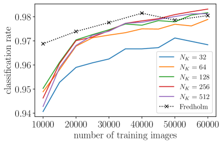
Figure 4. Results for the MNIST data set: Classification rates obtained from the Fredholm network over the number $M$ of training images in comparison with Keras networks with increasing number $N_{K}$ of nodes in the hidden layer.

Figure 4 shows the classification rates as obtained from our Fredholm network $\mathcal{G}\tilde{u}$ and of Keras networks of size $N_{K}=34,64,128,256,512$ on the fixed MNIST test data set of $m=10,000$ test images over the number $M$ of utilized training images. For the largest number of $M=60,000$ training data, the classification rates of the Keras networks are ranging from $0.9789$ to $0.9832$ for sufficiently large $N_{K}\geq 64$ and are thus comparable with the classification rate $0.9805$ of the Fredholm network. However, Keras networks are clearly outperformed for smaller sets of training data.

8. Conclusion and outlook

In this work, we have proposed a novel approach to function approximation and the training of large and high-dimensional shallow neural networks, based on their continuous asymptotic limit. Utilizing resulting Fredholm networks for function approximation and also for training in the original discrete case, we have thus traded highly nonlinear discrete training problems with finitely many unknown parameters for linear continuous training problems with infinitely many unknown values of a parameter function.

Fredholm training problems can be regarded as least-squares formulations of Fredholm integral equations of the first kind. They were solved approximately by Ritz-Galerkin discretization in combination with Tikhonov regularization and tensor train methods. Here, we particularly aimed at a significant reduction of memory consumption as well as computational costs to mitigate the curse of dimensionality as occurring for high-dimensional data. To this end, we described different tensor formats, suitable factorizations of kernel and basis functions as well as an alternating scheme for solving the tensorized linear training problems. Finally, we considered quasi Monte-Carlo sampling of discrete neural network parameters and introduced inductive importance sampling which is directly targeting the loss functional $\mathcal{J}_{N}$.

The predictive quality of the resulting approximatively trained Fredholm and neural networks are illustrated by numerical experiments with three well-established test problems of regression and classification type. The results clearly confirm that our approach is highly competitive with state-of-the-art neural network-based methods concerning efficiency and reliability. The investigations carried out in this work offer a number of further promising developments. In particular, numerical analysis of the whole approach will be subject of future research and will provide error estimates together with problem-oriented ansatz functions, more sophisticated regularization techniques, selection of tensor ranks, and further advanced sampling strategies.

Appendix A Factorization of ridge kernel functions

According to (2), ridge kernel functions $\psi\colon X\times Q\to\mathbb{R}$, are given by

$$\psi(x,\eta)=\sigma(w\cdot x+b),\quad\eta=(w,b)\in Q\subset\mathbb{R}^{s},\;s=d+1.$$

with hypercubes $X\in\mathbb{R}^{d}$, $Q=Q_{1}\times\cdots\times Q_{s}\subset\mathbb{R}^{s}$, and ridge activation function $\sigma:\mathbb{R}\mapsto\mathbb{R}$. Identifying $X$ with its embedding $\{(x,1)^{\top}\;|\;x\in X\}\subset\mathbb{R}^{s}$, ridge kernel functions take the form

$$\psi(x,\eta)=\sigma(x\cdot\eta).$$

In what follows, explicit tensor decompositons of different ridge activation functions are derived, either using the canonical format or TT format. In case of the latter, we use the core notation of the TT format [45] to represent FTT cores as two-dimensional arrays containing vector-valued functions as elements. More precisely, for a given functional tensor train $\hat{\mathbf{\Psi}}$ with cores $\hat{\mathbf{\Psi}}^{(k)}\in\mathbb{C}^{r_{k-1}\times M\times Q_{k}\times r_{k}}$ defined by

$$\hat{\mathbf{\Psi}}^{(k)}_{\ell_{k-1},i,\eta_{k},\ell_{k}}=\psi^{(k)}_{\ell_{k-1},\ell_{k}}(x_{i,k},\eta_{k})\colon\mathbb{R}\times Q_{k}\to\mathbb{C},$$

a single core is written as

(56) $$\left\llbracket\,\begin{matrix}\hat{\mathbf{\Psi}}^{(k)}\end{matrix}\,\right\rrbracket=\left\llbracket\,\begin{matrix}&&\\[-8.5359pt] \hat{\mathbf{\Psi}}^{(k)}_{1,:,\eta_{k},1}&\cdots&\hat{\mathbf{\Psi}}^{(k)}_{1,:,\eta_{k},r_{k}}\\ \vdots&\ddots&\vdots\\ \hat{\mathbf{\Psi}}^{(k)}_{r_{k-1},:,\eta_{k},1}&\cdots&\hat{\mathbf{\Psi}}^{(k)}_{r_{k-1},:,\eta_{k},r_{k}}\\[-9.95863pt] &&\end{matrix}\,\right\rrbracket,$$

where $\hat{\mathbf{\Psi}}^{(k)}_{\ell_{k-1},:,\eta_{k},\ell_{k}}=(\psi^{(k)}_{\ell_{k-1},\ell_{k}}(x_{i,k},\eta_{k}))_{i=1}^{M}$. Thus, the FTT decomposition of the auxiliary tensor $\hat{\mathbf{\Psi}}$, cf. (43), takes the form $\hat{\mathbf{\Psi}}=\left\llbracket\,\begin{matrix}\hat{\mathbf{\Psi}}^{(1)}\end{matrix}\,\right\rrbracket\otimes\dots\otimes\left\llbracket\,\begin{matrix}\hat{\mathbf{\Psi}}^{(s)}\end{matrix}\,\right\rrbracket$, denoting

$$\left(\left\llbracket\,\begin{matrix}\hat{\mathbf{\Psi}}^{(k)}\end{matrix}\,\right\rrbracket\otimes\left\llbracket\,\begin{matrix}\hat{\mathbf{\Psi}}^{(k+1)}\end{matrix}\,\right\rrbracket\right)_{\ell_{k-1},i_{k},\eta_{k},i_{k+1},\eta_{k+1},\ell_{k+1}}=\sum_{\ell_{k}=1}^{r_{k}}\hat{\mathbf{\Psi}}^{(k)}_{\ell_{k-1},i_{k},\eta_{k},\ell_{k}}\cdot\hat{\mathbf{\Psi}}^{(k+1)}_{\ell_{k},i_{k+1},\eta_{k+1},\ell_{k+1}}.$$

Proposition A.1.

Consider a monomial of the form $\psi(x,\eta)=(x\cdot\eta)^{p}$, $p\geq 0$, with $\eta\in Q$ and data points $x_{i}\in X$, $i=1,\dots,m$. The functional tensor $\mathbf{\Psi}\in\mathbb{R}^{M\times Q_{1}\times\cdots\times Q_{s}}$ defined by $\mathbf{\Psi}_{i,\eta_{1},\dots,\eta_{s}}=\psi(x_{i},\eta)$ can be written as $\mathbf{\Psi}=\Delta\cdot\hat{\mathbf{\Psi}}$, $\hat{\mathbf{\Psi}}\in\mathbb{R}^{M^{s}\times Q_{1}\times\dots\times Q_{s}}$, where

(57) $$\begin{split}\hat{\mathbf{\Psi}}=&~{}p!\left\llbracket\,\begin{matrix}\frac{1}{p!}(x_{:,1}\eta_{1})^{p}&\cdots&x_{:,1}\eta_{1}&e\end{matrix}\,\right\rrbracket\otimes\left\llbracket\,\begin{matrix}e&0&\cdots&0\\ x_{:,2}\eta_{2}&\ddots&\ddots&\vdots\\ \vdots&\ddots&\ddots&0\\ \frac{1}{p!}(x_{:,2}^{\prime}\eta_{2})^{p}&\cdots&x_{:,2}\eta_{2}&e\end{matrix}\,\right\rrbracket\otimes\cdots\\ &~{}\otimes\left\llbracket\,\begin{matrix}e&0&\cdots&0\\ x_{:,s-1}\eta_{s-1}&\ddots&\ddots&\vdots\\ \vdots&\ddots&\ddots&0\\ \frac{1}{p!}(x_{:,s-1}\eta_{s-1})^{p}&\cdots&x_{:,s-1}\eta_{s-1}&e\end{matrix}\,\right\rrbracket\otimes\left\llbracket\,\begin{matrix}e\\ x_{:,s}\eta_{s}\\ \vdots\\ \frac{1}{p!}(x_{:,s}\eta_{s})^{p}\end{matrix}\,\right\rrbracket\end{split}$$

with $e=(1,\dots,1)^{T}\in\mathbb{R}^{M}$.

Proof.

By using the multinomial formula, we know

$$\left(\sum_{k=1}^{s}z_{k}\right)^{p}=\sum_{\begin{subarray}{c}\ell_{1}+\dots+\ell_{s}=p\\ \ell_{1},\dots,\ell_{s}\geq 0\end{subarray}}\frac{p!}{\ell_{1}!\cdots\ell_{s}!}z_{1}^{\ell_{1}}\cdots z_{s}^{\ell_{s}}$$

for any $i\in\{1,\dots,M\}$. This can be written as a sequence of matrix multiplications of the form

$$\begin{split}\left(\sum_{k=1}^{s}z_{k}\right)^{p}=&~{}p!\begin{bmatrix}z_{1}^{p}&\cdots&z_{1}^{0}\end{bmatrix}\begin{bmatrix}\displaystyle\sum_{\ell_{2}+\dots+\ell_{s}=0}\frac{1}{\ell_{2}!\cdots\ell_{s}!}z_{2}^{\ell_{2}}\cdots z_{s}^{\ell_{s}}\\ \vdots\\ \displaystyle\sum_{\ell_{2}+\dots+\ell_{s}=p}\frac{1}{\ell_{2}!\cdots\ell_{s}!}z_{2}^{\ell_{2}}\cdots z_{s}^{\ell_{s}}\end{bmatrix}\\ =&~{}p!\begin{bmatrix}z_{2}^{p}&\cdots&z_{2}^{0}\end{bmatrix}\begin{bmatrix}z_{2}^{0}&&0\\ \vdots&\ddots&\\ z_{2}^{p}&\cdots&z_{2}^{0}\end{bmatrix}\begin{bmatrix}\displaystyle\sum_{\ell_{3}+\dots+\ell_{s}=0}\frac{1}{\ell_{3}!\cdots\ell_{s}!}z_{3}^{\ell_{3}}\cdots z_{s}^{\ell_{s}}\\ \vdots\\ \displaystyle\sum_{\ell_{3}+\dots+\ell_{s}=p}\frac{1}{\ell_{3}!\cdots\ell_{s}!}z_{3}^{\ell_{3}}\cdots z_{s}^{\ell_{s}}\end{bmatrix}\\ =&~{}\dots\\ =&~{}p!\begin{bmatrix}z_{2}^{p}&\cdots&z_{2}^{0}\end{bmatrix}\begin{bmatrix}z_{2}^{0}&&0\\ \vdots&\ddots&\\ z_{2}^{p}&\cdots&z_{2}^{0}\end{bmatrix}\cdots\begin{bmatrix}z_{s-1}^{0}&&0\\ \vdots&\ddots&\\ z_{s-1}^{p}&\cdots&z_{s-1}^{0}\end{bmatrix}\begin{bmatrix}z_{s}^{0}\\ \vdots\\ z_{s}^{p}\end{bmatrix}.\end{split}$$

Thus, for $\mathbf{\Psi}=\Delta\hat{\mathbf{\Psi}}$ with $\hat{\mathbf{\Psi}}$ as given in (57), we get

$$\begin{split}\mathbf{\Psi}_{i,\eta_{1},\dots,\eta_{s}}=&~{}\sum_{j_{1}=1}^{M}\dots\sum_{j_{s}=1}^{M}\Delta_{i,j_{1},\dots,j_{s}}\hat{\mathbf{\Psi}}_{j_{1},\dots,j_{s},\eta_{1},\dots,\eta_{s}}\\ =&~{}\sum_{j_{1}=1}^{M}\dots\sum_{j_{s}=1}^{M}\delta_{i,j_{1}}\cdots\delta_{i,j_{s}}\hat{\mathbf{\Psi}}_{j_{1},\dots,j_{s},\eta_{1},\dots,\eta_{s}}\\ =&~{}\hat{\mathbf{\Psi}}_{i,\dots,i,\eta_{1},\dots,\eta_{s}}=\left(\sum_{k=1}^{s}x_{i,k}\eta_{k}\right)^{p}=(x_{i}\cdot\eta)^{p}.\qed\end{split}$$

A.1. Trivial activation function

In the simplest case $\sigma=\text{Id}$, the ridge kernel function is bilinear, i.e., $\psi(x,\eta)=x\cdot\eta$, and clearly can be written in the form (42) (see Example 5.3). Let us consider the functional tensor

$${\mathbf{\Psi}}\in\mathbb{R}^{M\times Q_{1}\times\cdots\times Q_{s}},\qquad\mathbf{\Psi}_{i,\eta_{1},\dots,\eta_{s}}=x_{i}\cdot\eta=\sum_{k=1}^{s}x_{i,k}\eta_{k},\qquad s=d,$$

associated to $\psi$ according to (41) for the given data points $x_{i}\in X$, $i=1,\dots,M$. It can be expressed as $\mathbf{\Psi}=\Delta\cdot\hat{\mathbf{\Psi}}$, see Proposition 5.5, where the auxiliary tensor $\hat{\mathbf{\Psi}}$ has the functional canonical decomposition

(58) $$\hat{\mathbf{\Psi}}=\eta_{1}\begin{pmatrix}x_{1,1}\\ \vdots\\ x_{M,1}\end{pmatrix}\otimes\begin{pmatrix}1\\ \vdots\\ 1\end{pmatrix}\otimes\dots\otimes\begin{pmatrix}1\\ \vdots\\ 1\end{pmatrix}~{}+~{}\cdots~{}+~{}\begin{pmatrix}1\\ \vdots\\ 1\end{pmatrix}\otimes\dots\otimes\begin{pmatrix}1\\ \vdots\\ 1\end{pmatrix}\otimes\eta_{d}\begin{pmatrix}x_{1,d}\\ \vdots\\ x_{M,d}\end{pmatrix}$$

Using the core notation (56) and Proposition A.1, we can also represent $\hat{\mathbf{\Psi}}$ as a functional tensor train:

(59) $$\hat{\mathbf{\Psi}}=\left\llbracket\,\begin{matrix}x_{:,1}\eta_{1}&e\end{matrix}\,\right\rrbracket\otimes\left\llbracket\,\begin{matrix}e&0\\ x_{:,2}\eta_{2}&e\end{matrix}\,\right\rrbracket\otimes\dots\otimes\left\llbracket\,\begin{matrix}e&0\\ x_{:,d-1}\eta_{d-1}&e\end{matrix}\,\right\rrbracket\otimes\left\llbracket\,\begin{matrix}e\\ x_{:,d}\eta_{d}\end{matrix}\,\right\rrbracket.$$

Note that the canonical rank of (58) is equal to $d$ whereas the FTT ranks $r_{1},\dots,r_{d-1}$ of (59) are always equal to $2$ for any state space dimension $d$.

A.2. Logistic activation function

For the logistic activation function $\sigma_{\kappa}$ given in (4), the kernel function takes the form

(60) $$\psi_{\kappa}(x,\eta)=\frac{\exp(\kappa\,x\cdot\eta)}{1+\exp(\kappa\,x\cdot\eta))}=\frac{1}{1+\exp(-\kappa\,x\cdot\eta)}=\frac{1}{2}+\frac{1}{2}\tanh\left(\frac{-\kappa\,x\cdot\eta}{2}\right).$$

We expand $\sigma_{\kappa}(z)$ into a Taylor series at $z=0$, to obtain

(61) $$\psi_{\kappa}(x,\eta)=\frac{1}{2}+\frac{\kappa\,x\cdot\eta}{4}-\frac{\kappa^{3}\,(x\cdot\eta)^{3}}{48}+O(x\cdot\eta)^{5}.$$

Assuming that the side lengths of $Q$ are sufficiently small, we skip the quintic part in (61). The resulting approximation of $\psi_{\kappa}$ can be written in the form of (42) with $r=1+s+\frac{1}{6}(s^{3}+3s^{2}+2s)$. Indeed, the zero- and the first-order term in (61) can be written as a functional canonical tensor with rank $1+s$ summands, cf. (58), while, by the multinomial formula, the cubic term can be written as

$$\frac{\kappa^{3}\,(x\cdot\eta)^{3}}{48}=\frac{\kappa^{3}}{48}\left(\sum_{k=1}^{s}x_{k}\eta_{k}\right)^{3}=\frac{\kappa^{3}}{48}\sum_{\ell_{1}+\dots+\ell_{s}=3}\frac{6}{\ell_{1}!\cdots\ell_{s}!}(x_{1}\eta_{1})^{\ell_{1}}\cdots(x_{s}\eta_{s})^{\ell_{s}}$$

with $\sum_{k_{3}=1}^{s}\sum_{k_{2}=1}^{k_{3}}\sum_{k_{1}=1}^{k_{2}}1=\frac{1}{6}(s^{3}+3s^{2}+2s)$ summands. In contrast to that, the ranks of the corresponding FTT decomposition are always bounded by $4$ for any parameter dimension $s$. This can be seen by using Proposition A.1 for each of the first three terms in (61) and adding the respective decompositions. The resulting FTT representation of the auxiliary tensor is then given by

$$\begin{split}\hat{\mathbf{\Psi}}=&\left\llbracket\,\begin{matrix}\frac{1}{6}(\eta_{1}x_{:,1})^{3}&\frac{1}{2}(\eta_{1}x_{:,1})^{2}&\eta_{1}x_{:,1}&e\end{matrix}\,\right\rrbracket\otimes\left\llbracket\,\begin{matrix}e&0&0&0\\ \eta_{2}x_{:,2}&e&0&0\\ \frac{1}{2}(\eta_{2}x_{:,2})^{2}&\eta_{2}x_{:,2}&e&0\\ \frac{1}{6}(\eta_{2}x_{:,2})^{3}&\frac{1}{2}(\eta_{2}x_{:,2})^{2}&\eta_{2}x_{:,2}&e\end{matrix}\,\right\rrbracket\otimes\dots\\ &\otimes\left\llbracket\,\begin{matrix}e&0&0&0\\ \eta_{d-1}x_{:,{d-1}}&e&0&0\\ \frac{1}{2}(\eta_{d-1}x_{:,{d-1}})^{2}&\eta_{d-1}x_{:,{d-1}}&e&0\\ \frac{1}{6}(\eta_{d-1}x_{:,{d-1}})^{3}&\frac{1}{2}(\eta_{d-1}x_{:,{d-1}})^{2}&\eta_{d-1}x_{:,{d-1}}&e\end{matrix}\,\right\rrbracket\otimes\left\llbracket\,\begin{matrix}-\frac{\kappa^{3}}{8}e\\ -\frac{\kappa^{3}}{8}\eta_{d}x_{:,{d}}\\ -\frac{\kappa^{3}}{16}(\eta_{d}x_{:,{d}})^{2}+\frac{\kappa}{4}e\\ -\frac{\kappa^{3}}{48}(\eta_{d}x_{:,{d}})^{3}+\frac{\kappa}{4}\eta_{d}x_{:,{d}}+\frac{1}{2}e\end{matrix}\,\right\rrbracket.\end{split}$$

A.3. Heaviside activation function

For each fixed $z\in\mathbb{R}$ and $\kappa\to\infty$ the logistic activation function $\sigma_{\kappa}(z)$ converges to the Heaviside function $\sigma_{\infty}(z)$ defined in (3). However, as the interval of convergence $[-\frac{\pi}{\kappa},\frac{\pi}{\kappa}]$ of the Taylor expansion (61) shrinks with incresing $\kappa$, we now derive a different kind of approximation of the Heaviside kernel function $\psi_{\infty}(x,\eta)=\sigma_{\infty}(x\cdot\eta)$ of the form (42). Our starting point is the Fourier epansion

$$\sigma_{\infty}(z)=\frac{1}{2}+\frac{2}{\pi}\sum_{\ell=1}^{\infty}\frac{1}{2\ell-1}\sin\left(\frac{(2\ell-1)\pi}{T}z\right),$$

which converges pointwise within the interval $[-T,T]$ for suitable $T>0$. Euler’s formula $\sin(z)=(\exp(\mathrm{i}z)-\exp(-\mathrm{i}z))/2\mathrm{i}$ yields

$$\sigma_{\infty}(z)=\frac{1}{2}+\frac{1}{\pi\mathrm{i}}\sum_{\ell=1}^{\infty}\frac{1}{2\ell-1}\left(\exp\left(\frac{(2\ell-1)\pi\mathrm{i}}{T}z\right)-\exp\left(-\frac{(2\ell-1)\pi\mathrm{i}}{T}z\right)\right).$$

Inserting $z=x\cdot\eta$, we obtain the representation

$$\psi_{\infty}(x,\eta)=\frac{1}{2}+\frac{1}{\pi\mathrm{i}}\sum_{\ell=1}^{\infty}\frac{1}{2\ell-1}\left(\prod_{k=1}^{d}\exp\left(\frac{(2\ell-1)\pi\mathrm{i}}{T}x_{k}\eta_{k}\right)-\prod_{k=1}^{d}\exp\left(-\frac{(2\ell-1)\pi\mathrm{i}}{T}x_{k}\eta_{k}\right)\right)$$

of the Heaviside kernel function for $x\cdot\eta\in[-T,T]$. Truncating this expansion at $\ell=\ell_{0}$, we obtain the desired factorization (42) of the resulting approximation with $r=2\ell_{0}+1$ summands. In this case, the decomposition (44) of the associated functional tensor $\mathbf{\Psi}$ reads

$$\begin{split}\mathbf{\Psi}&=\Delta\cdot\left[\frac{1}{2}\bigotimes_{k=1}^{d}e~{}+~{}\frac{1}{\pi\mathrm{i}}\sum_{\ell=1}^{\ell_{0}}\frac{1}{2\ell-1}\bigotimes_{k=1}^{d}\exp\left(\frac{(2\ell-1)\pi\mathrm{i}}{T}\eta_{k}x_{:,k}\right)\right.\\ &\qquad\qquad\left.-~{}\frac{1}{\pi\mathrm{i}}\sum_{\ell=1}^{\ell_{0}}\frac{1}{2\ell-1}\bigotimes_{k=1}^{d}\exp\left(-\frac{(2\ell-1)\pi\mathrm{i}}{T}\eta_{k}x_{:,k}\right)\right].\end{split}$$

References

- [1] Shun-ichi Amari. Backpropagation and stochastic gradient descent method. Neurocomputing, 5(4-5):185–196, 1993.
- [2] Léon Bottou. Stochastic gradient descent tricks. In Neural networks: Tricks of the trade, pages 421–436. Springer, 2012.
- [3] Patrick Cheridito, Arnulf Jentzen, and Florian Rossmannek. Non-convergence of stochastic gradient descent in the training of deep neural networks. Journal of Complexity, 64:101540, 2021.
- [4] Qipin Chen and Wenrui Hao. Randomized Newton’s method for solving differential equations based on the neural network discretization. Journal of Scientific Computing, 92(2):1–22, 2022.
- [5] Andrew R. Conn, Nicholas I. M. Gould, and Philippe L. Toint. Trust region methods. SIAM, 2000.
- [6] Eiji Mizutani and James W. Demmel. On structure-exploiting trust-region regularized nonlinear least squares algorithms for neural-network learning. Neural Networks, 16(5-6):745–753, 2003.
- [7] Alena Kopanicáková and Rolf Krause. Globally convergent multilevel training of deep residual networks. SIAM Journal on Scientific Computing, pages S254–S280, 2022. doi:https://doi.org/10.1137/21M1434076.
- [8] Grant M. Rotskoff and Eric Vanden-Eijnden. Trainability and accuracy of neural networks: An interacting particle system approach, 2019. arXiv:1805.00915.
- [9] Qichao Que and Mikhail Belkin. Back to the future: Radial basis function networks revisited. In Artificial intelligence and statistics, pages 1375–1383. PMLR, 2016.
- [10] Qichao Que, Mikhail Belkin, and Yusu Wang. Learning with Fredholm kernels. Advances in neural information processing systems, 27, 2014.
- [11] Wei Wang, Hao Wang, Zhaoxiang Zhang, Chen Zhang, and Yang Gao. Semi-supervised domain adaptation via Fredholm integral based kernel methods. Pattern Recognition, 85:185–197, 2019.
- [12] Qichao Que and Mikhail Belkin. Inverse density as an inverse problem: The Fredholm equation approach. Advances in neural information processing systems, 26, 2013.
- [13] Martin Hanke Heinz W. Engl and Andreas Neubauer. Regularization of Inverse Problems. Kluwer Academic Publishers, Dordrecht, Netherlands, 1996.
- [14] Sebastian Holtz, Thorsten Rohwedder, and Reinhold Schneider. The alternating linear scheme for tensor optimization in the tensor train format. SIAM Journal on Scientific Computing, 34(2):A683–A713, 2012. doi:10.1137/100818893.
- [15] Stefan Klus and Patrick Gelß. Tensor-based algorithms for image classification. Algorithms, 12(11), 2019. doi:10.3390/a12110240.
- [16] Volker Lohweg, Jan Leif Hoffmann, Helene Dörksen, Roland Hildebrand, Eugen Gillich, Jürg Hofmann, and Johannes Schaede. Banknote authentication with mobile devices. In Adnan M. Alattar, Nasir D. Memon, and Chad D. Heitzenrater, editors, Media Watermarking, Security, and Forensics 2013, volume 8665, page 866507. International Society for Optics and Photonics, SPIE, 2013. doi:10.1117/12.2001444.
- [17] I-Cheng Yeh. Modeling of strength of high-performance concrete using artificial neural networks. Cement and Concrete Research, 28(12):1797–1808, 1998. doi:10.1016/S0008-8846(98)00165-3.
- [18] I-Cheng Yeh. Prediction of strength of fly ash and slag concrete by the use of artificial neural networks. J. Chin. Inst. Civil Hydraul. Eng., 15:659–663, 2003.
- [19] I-Cheng Yeh. Analysis of strength of concrete using design of experiments and neural networks. Journal of Materials in Civil Engineering, 18(4):597–604, 2006. doi:10.1061/(ASCE)0899-1561(2006)18:4(597).
- [20] Syyed Adnan Raheel Shah, Marc Azab, Hany M. Seif ElDin, Osama Barakat, Muhammad Kashif Anwar, and Yasir Bashir. Predicting compressive strength of blast furnace slag and fly ash based sustainable concrete using machine learning techniques: An application of advanced decision-making approaches. Buildings, 12(7), 2022. doi:10.3390/buildings12070914.
- [21] Yann Lecun, Léon Bottou, Yoshua Bengio, and Patrick Haffner. Gradient-based learning applied to document recognition. Proceedings of the IEEE, 86(11):2278–2324, 1998. doi:10.1109/5.726791.
- [22] Allan Pinkus. Approximation theory of the mlp model in neural networks. Acta numerica, 8:143–195, 1999.
- [23] Bekir Karlik and A Vehbi Olgac. Performance analysis of various activation functions in generalized MLP architectures of neural networks. International Journal of Artificial Intelligence and Expert Systems, 1:111–122, 2011.
- [24] Tianping Chen and Hong Chen. Approximation capability to functions of several variables, nonlinear functionals, and operators by radial basis function neural networks. IEEE Transactions on Neural Networks, 6(4):904–910, 1995.
- [25] Maxwell Stinchcombe and Halbert White. Approximating and learning unknown mappings using multilayer feedforward networks with bounded weights. In 1990 IJCNN International Joint Conference on Neural Networks, pages 7–16. IEEE, 1990.
- [26] Rainer Kress. Linear Integral Equations. Springer-Verlag, New York, 1999.
- [27] Charles W. Groetsch. The theory of Tikhonov regularization for Fredholm equations of the first kind. Pitman Publishing Limited, London, 1984.
- [28] George Cybenko. Approximation by superpositions of a sigmoidal function. Math. Control Signal Systems, 2:303–314, 1989. doi:10.1007/BF02551274.
- [29] Frank L Hitchcock. The expression of a tensor or a polyadic as a sum of products. Journal of Mathematics and Physics, 6(1-4):164–189, 1927.
- [30] Ivan V. Oseledets and Eugene E. Tyrtyshnikov. Breaking the curse of dimensionality, or how to use SVD in many dimensions. SIAM Journal on Scientific Computing, 31(5):3744–3759, 2009.
- [31] Ivan V. Oseledets. Tensor-train decomposition. SIAM Journal on Scientific Computing, 33(5):2295–2317, 2011. doi:10.1137/090752286.
- [32] Antonio Falcó and Wolfgang Hackbusch. On minimal subspaces in tensor representations. Foundations of computational mathematics, 12(6):765–803, 2012.
- [33] Sebastian Holtz, Thorsten Rohwedder, and Reinhold Schneider. On manifolds of tensors of fixed TT-rank. Numerische Mathematik, 120(4):701–731, 2012.
- [34] Tamara G. Kolda and Brett W. Bader. Tensor decompositions and applications. SIAM review, 51(3):455–500, 2009.
- [35] Wolfgang Hackbusch. Tensor spaces and numerical tensor calculus, volume 42. Springer, 2012.
- [36] Alex Gorodetsky, Sertac Karaman, and Youssef Marzouk. A continuous analogue of the tensor-train decomposition. Computer Methods in Applied Mechanics and Engineering, 347:59–84, 2019. doi:10.1016/j.cma.2018.12.015.
- [37] Patrick Gelß. The tensor-train format and its applications: Modeling and analysis of chemical reaction networks, catalytic processes, fluid flows, and Brownian dynamics. PhD thesis, FU Berlin, 2017.
- [38] Patrick Gelß, Stefan Klus, Jens Eisert, and Christof Schütte. Multidimensional approximation of nonlinear dynamical systems. Journal of Computational and Nonlinear Dynamics, 14(6):061006, 2019. doi:10.1115/1.4043148.
- [39] Kim Batselier. Enforcing symmetry in tensor network MIMO Volterra identification. IFAC-PapersOnLine, 54(7):469–474, 2021. doi:10.1016/j.ifacol.2021.08.404.
- [40] Sergey V. Dolgov and Dmitry V. Savostyanov. Alternating minimal energy methods for linear systems in higher dimensions. SIAM Journal on Scientific Computing, 36(5):A2248–A2271, 2014. doi:10.1137/140953289.
- [41] Lars Grasedyck and Sebastian Krämer. Stable ALS approximation in the TT-format for rank-adaptive tensor completion. Numerische Mathematik, 143:855–904, 2019. doi:10.1007/s00211-019-01072-4.
- [42] Thorsten Rohwedder and André Uschmajew. On local convergence of alternating schemes for optimization of convex problems in the tensor train format. SIAM Journal on Numerical Analysis, 51(2):1134–1162, 2013. doi:10.1137/110857520.
- [43] Mike Espig, Wolfgang Hackbusch, and Aram Khachatryan. On the convergence of alternating least squares optimisation in tensor format representations, 2015. arXiv:1506.00062.
- [44] Benjamin A. Young, Alex Hall, Laurent Pilon, Puneet Gupta, and Gaurav Sant. Can the compressive strength of concrete be estimated from knowledge of the mixture proportions?: New insights from statistical analysis and machine learning methods. Cement and Concrete Research, 115:379–388, 2019. doi:10.1016/j.cemconres.2018.09.006.
- [45] Patrick Gelß, Stefan Klus, Sebastian Matera, and Christof Schütte. Nearest-neighbor interaction systems in the tensor-train format. Journal of Computational Physics, 341:140–162, 2017.