Classifying the universal coarsening dynamics of a quenched ferromagnetic condensate

Abstract

Scale invariance and self-similarity in physics provide a unified framework to classify phases of matter and dynamical properties of near-equilibrium systems. However, extending this framework to far-from-equilibrium quantum many-body systems and categorizing their dynamics have remained a major challenge in physics. Here, we report on the first classification of universal coarsening dynamics in a quenched two-dimensional ferromagnetic spinor Bose gas. We observe spatiotemporal scaling of spin correlation functions with distinguishable scaling exponents, $1/z=0.58(2)$ and $1/z=0.43(2)$, characteristic, respectively, of binary and diffusive fluids. We find the universality class of the coarsening dynamics are determined by the symmetry of the order parameters and the annihilation dynamics of the topological defects. These observations are in excellent agreement with many-body simulations. Our results represent a paradigmatic example of categorizing far-from-equilibrium dynamics in quantum many-body systems.

Critical phenomena occur at the points of second order phase transitions in classical and quantum systems, where the correlation length, which determines the fluctuations in the size boundaries between different phases, diverges [1, 2]. Critical opalescence, first observed in the gas-liquid transition in carbon dioxide, renders the transparent liquid murky because the density fluctuations in the liquid become of the order of the wavelength of light. In quantum systems, examples are the Ising magnets, Curie transitions in ferromagnets, and Bose-Einstein condensates. Such static critical phenomena can be divided into universality classes, each class described by same set of exponents. It was realized that two systems belonging to the same static universality class may belong to different dynamic classes [3]. The first direct measurement of the divergence of the correlation length in an inhomogeneous BEC in the thermodynamic limit was performed in [4].

Understanding and classifying the universality classes in the far from equilibrium dynamics of closed quantum many-body systems remain outstanding challenges in physics [5, 6, 7]. Although many aspects of isolated quantum systems are fundamentally different from those of traditional systems with thermal baths [3, 8], far out-of-equilibrium quantum systems can display universal behavior on approach to thermal equilibrium [9, 10, 11, 12, 13, 14, 15]. Recent theories [16, 17, 18, 19, 20, 21] have proposed a comprehensive picture of the emerging universal dynamics, where a system driven far from equilibrium undergoes critical slowing down and displays self-similar time evolution associated with nonthermal fixed points.

Ultracold atomic quantum simulators have been ideal platforms for studying universal dynamics because of their high degree of isolation from the environment and exquisite parameters and interactions controllability [5, 6, 7]. Recent experiments in one-dimensional Bose gas have observed spatiotemporal scaling of the structure factor of the spin correlation functions [11] and the momentum distribution of the atomic cloud [12]. In a three-dimensional homogeneous system, dynamic scaling is observed in both the infrared and ultraviolet regimes [13]. Despite these findings, the scaling exponents do not agree with the nonthermal universality classes [22, 23, 21, 24], leaving open the question of what determines the universal scaling exponents in nonequilibrium quantum systems and how to classify the far from equilibrium dynamics in these systems.

Here, we observe universal coarsening dynamics in a quenched strongly ferromagnetic superfluid in two dimensions (2D). We demonstrate that universality can be classified by: i) the symmetry of the order parameter in the post-quench phase and ii) the merging and annihilation dynamics of the associated topological defects, such as domain walls and vortices. Quenching the quadratic Zeeman energy (QZE), magnetic domains of relatively small size are spontaneously generated and subsequently merge entering the coarsening stage in the long time-evolution. Monitoring the spin correlation functions at various hold times, we confirm that the dynamics is self-similar regardless of varying experimental conditions. Specifically, when the ground state after the quench has $\mathbb{Z}_{2}$ (spin inversion) symmetry, the domain growth dynamics can be described by the universal scaling exponent $1/z\simeq 0.58(2)$. At high-momentum – the so-called “Porod tail” [8] – is also observed in the structure factor as an imprint of the universal character of the dynamics, associated with magnetic domain formation with sharp edges. The results show that the emergent dynamics belongs to a binary fluid universality class in the inertial hydrodynamic regime [3, 25, 26]. Tuning the Hamiltonian to have SO(3), i.e. spin rotation symmetry, the characteristics of the ensuing magnetic domain coarsening are modified. In the diffusive growth dynamics of domain length [27], the scaling exponent is $1/z\simeq 0.43(3)$, which belongs to the nonthermal universality class of O$(N)$ symmetric Hamiltonian [21, 24]. Utilizing matter-wave interferometry, we identify the formation of spin vortices and argue that their annihilation is closely related to the observed diffusive dynamics.

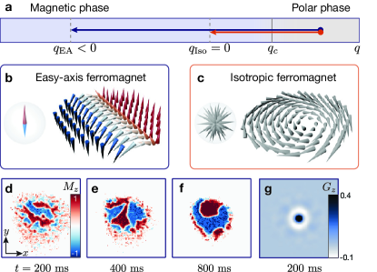
Figure 1: Universal coarsening dynamics and topological defects. a, Schematic diagram of the experimental sequence. Ramping the quadratic Zeeman energy $q$, the initially prepared polar condensate is quenched to a magnetic phase ($q<q_{c}$). Universal coarsening dynamics are investigated at (i) $q_{\rm EA}<0$ easy-axis phases with $\mathbb{Z}_{2}$ spin symmetry and (ii) $q_{\rm Iso}=0$ isotropic ferromagnetic phase with SO(3) symmetry. b, Magnetic domain in the easy-axis ferromagnetic phase. c, Spin texture of the spin vortex in the isotropic ferromagnetic phase. The magnetization vector in each regime are shown on the left side of the defects in terms of spin sphere. d-f,, Snap shot images of magnetization at various hold times after quenching the polar condensate to easy-axis phase, $q_{\rm EA}/h=-200~{}\rm Hz$. g, Correlation function of longitudinal magnetization $G_{z}(x,y)$ at $t=200$ ms. The data is averaged over 100 experimental realizations.

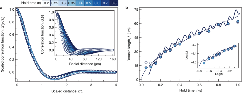
Figure 2: Dynamic scaling and power law growth of the domain length. a, Scaled correlation function $\mathcal{G}(r/L)$ at various hold times, $t\in[0.2~{}\rm s,0.8~{}\rm s]$. Longitudinal spin correlation functions at various hold times (inset) collapse onto a single function after rescaling the radial position by a characteristic length $L(t)$. The domain size $L(t)$ is set by a distance with $G_{z}(r,t)=0$. The solid line represents the numerical result when using the experimental parameters. b, Power law growth of the domain length $L(t)$. Data with closed (open) circles represent rescaled domain length after (without) deconvolution. The solid line is the theory line. The oscillatory behavior comes from the breathing motion of the condensates. Small deviations observed at long evolution times ($t\sim 1$ s) between the theory and experiment are attributed to atom losses by microwave dressing. The dashed line represents a power law function $L(t)\sim t^{1/z}$ with $1/z=0.61$, which is obtained from a linear fit in the log-log plot of the domain growth dynamics (inset). Each data point is obtained with more than 100 independent experimental runs, and one standard error of the mean (s.e.m) is smaller than the data point.

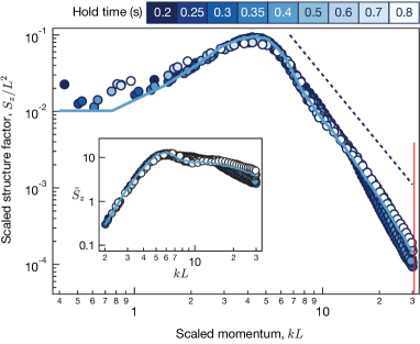
Figure 3: Dynamic scaling of the spin structure factor in the easy-axis quench. The structure factor of longitudinal magnetization $S_{z}(k,t)$ is rescaled by the domain length: $S_{z}\rightarrow S_{z}/L^{2}$ and $k\rightarrow kL$. The dashed line is the universal Porod tail $S_{z}(k,t)\sim k^{-3}$ with an offset for clarity. The vertical line (red) represents the momentum resolution for $t=0.2~{}\rm s$. Inset shows the structure factor with compensation, $\tilde{S}_{z}=S_{z}(k,t)Lk^{3}$. The solid line is the numerically calculated structure factor after rescaling.

Our experiments begin with preparing a 2D degenerate spin-1 Bose gas of ⁷Li atoms in an optical dipole trap [28] experiencing a finite magnetic field. As such the condensate is in the polar phase, where all atoms reside in the $m_{z}=0$ hyperfine level [29]. To initiate the nonequilibrium dynamics, we switch on the microwave field that quenches the quadratic Zeeman energy from $q/h=510$ Hz (polar phase) to a final value (Fig. 1a). This allows to dynamically cross the phase boundaries and thus renders the initial polar state unstable, forming magnetic domains. [30]. After a hold time $t$, we measure the in-situ atomic density for each spin state and record the magnetization either along the vertical $M_{z}$ or the horizontal spin axis $M_{x}$ [29]. A key feature of our system is the strongly ferromagnetic spin interactions [28], such that the characteristic time (length) scale is much shorter (smaller) compared to other alkali atomic systems. For instance, the spin interaction energy is $c\simeq-h\times 160\rm~{}Hz$ and characteristic time scale for domain formation is $t_{s}=\hbar/2\absolutevalue{c}\simeq 0.5~{}\rm{ms}$ [30]. Such strong interaction makes it possible to monitor the spinor gas for evolution times $t\simeq 2\times 10^{3}~{}t_{s}\simeq 1$ s, being long enough to study the emergent universal coarsening dynamics [25, 31, 26, 27]. To validate the experimental observations, we perform extensive numerical simulations of the underlying Gross-Pitaevskii equations tailored to the experimental setup. The truncated Wigner approximation is employed [32] accounting for quantum and thermal fluctuations in the initial polar state [29].

We first investigate the nonequilibrium dynamics in the easy-axis ferromagnetic phase, $q_{\rm EA}/h=-200~{}\rm{Hz}$. The order parameter in the easy-axis has $U(1)\times\mathbb{Z}_{2}$ symmetry supporting the formation of magnetic domain walls as topological defects (Fig. 1b). After the quench, the polar phase is dynamically unstable and atom pairs with $\ket{F=1,m_{z}=\pm 1}$ ($\ket{\pm 1}$) spin states and opposite momenta are generated. The kinetic energy, $\varepsilon_{k}$, of the created spin states stems from the post-quench QZE and the associated spin interaction energy, $\varepsilon_{k}=-q_{\rm EA}-c$ [33, 34]. Since the kinetic energy is comparable to the condensate chemical potential $\mu/h=310~{}\rm{Hz}$, we can assure that the spinor gas is driven far from equilibrium. At early times, $t<10$ ms, spin-mixing takes place and the populations of the spin $\ket{\pm 1}$ states increase exponentially reaching a steady value after 100 ms. In the course of the spin-mixing process gauge vortices appear in the $\ket{\pm 1}$ states, which either annihilate or drift out of the condensate, giving their place to magnetic domains [29]. Afterward, the number of spin domains decreases and their size increases, resulting in a process known as coarsening dynamics (Fig 1d-f). During the coarsening dynamics, the time-evolution displays a self-similar behavior characterized by a universal scaling law where the condensate is away from both its initial and equilibrium state. For longer evolution times ($t\sim 2$ s), only a few domains are left, and coarsening is terminated [29].

The scaling behavior can be understood by analyzing the equal time correlation function of the longitudinal magnetization [26], $G_{z}(\mathbf{r},t)=\frac{1}{\mathscr{N}}\int d^{2}\mathbf{r^{\prime}}\langle M_{z}(\mathbf{r+r^{\prime}},t)M_{z}(\mathbf{r^{\prime}},t)\rangle$ depicted in Fig. 1g. Here, $\mathbf{r}=(x,y)$ and $\mathscr{N}=\int d^{2}\mathbf{r^{\prime}}\langle M_{z}(\mathbf{r^{\prime}},t)^{2}\rangle$ is the normalization factor. In the inset of Fig. 2a, we present the radial profile of the spin correlation functions $G_{z}(r,t)$ at various hold times. The anti-correlation captured by $G_{z}(r,t)$ indicates the creation of magnetic domains in opposite spin states. We quantify, both in theory and experiment, the average domain size $L(t)$ as the first zero of the correlation function, $G_{z}(L,t)=0$ [26]. Indeed, upon rescaling the radial distance, $r\rightarrow r/L(t)$, the correlation function at various hold times collapses onto a single curve, $\mathcal{G}[r/L(t)]$ (Fig. 2a), indicating the self-similar character of the universal dynamics.

The universal growth dynamics is characterized by the power law increase of the domain length $L(t)\sim t^{1/z}$ (Fig. 2b), where the dynamical critical exponent $1/z$ determines the universality class of the emergent coarsening dynamics. Since in the easy-axis phase, the spinor gas reduces to a binary superfluid system consisting of only the $m_{z}=\pm 1$ components, the coarsening dynamics belongs to a binary fluid universality class or Model H [3]. Previous numerical studies operating in the thermodynamic limit indeed confirmed this argument and predicted the scaling exponent to be $1/z=2/3$ [25, 31, 26].

Figure 2b shows the power law growth of $L(t)$ as extracted from both experiment and theory. The scaling exponent in the experiment (open circles) is $1/z=0.57(2)$, which is in excellent agreement with our mean-field simulations $1/z_{\rm sim}\simeq 0.59(1)$ using the experimental parameters. Here, the time interval for the scaling regime is set to $t\in[0.2~{}\rm s,0.8~{}\rm s]$, and the independency of the scaling exponent on the time interval is presented [29]. The exponents as found both experimentally and theoretically, however, are smaller than the predicted thermodynamic limit value $1/z=2/3$ [25, 31, 26], and we attribute this discrepancy to the finite size of our system enforced by the external trap. While the universal scaling arguments are strictly valid in the thermodynamic limit, finite size corrections should reduce the exponent as, $1/z\simeq 2/3(1-\mathcal{O}(\xi_{s}/L))$ [35, 31], where $\xi_{s}=\hbar/\sqrt{2m\absolutevalue{c}}\simeq 2.2~{}\mu{}m$ is the spin healing length. Furthermore, our imaging system has an effective resolution of $5~{}\mu{}m$ that could increase the domain length. Employing the Weiner deconvolution method, we recalibrate the domain size and obtain $1/z=0.61(3)$. Similar universal behavior is observed in counting the magnetic domain number after the quench [29].

Dynamical scaling is also represented in the structure factor, $S_{z}({k},t)=L(t)^{2}S_{u}({k}L(t))$, which is the fourier transformation of the spin correlation function, with a scaling function $S_{u}$ [26]. The scaling form is identical to the nonthermal fixed theory that suggests $S_{z}(k,t)=t^{d/z}f_{S}(t^{1/z}k)$ in $d$ spatial dimensions, and a scaling function $f_{S}$ [16, 17, 18, 19, 20, 21]. In Fig. 3, we provide the rescaled structure factors within the time interval $t\in[0.2~{}\rm s,0.8~{}s]$. A universal scaling of the Porod tail, $S_{z}(k)\sim k^{-3}$ is observed [8]. At early times ($t<100~{}\rm ms$), we observe that the structure factor monotonically decreases (not shown), and only after the system enters the coarsening stage the characteristic “knee” shape and the universal high-momentum tail are revealed. The $k^{-3}$ scaling behavior originates from a linear decay of the correlation function with sharp domain wall edges among the $m_{z}=\pm 1$ states [8], which is confirmed in our experiment by imaging the $M_{z}$ and $M_{x}$ [29].

To demonstrate universality, we further investigate the quench dynamics with three different experimental configurations (Fig. 4a): (i) We take an equal superposition of $\ket{\pm 1}$ states at $q/h=510~{}\rm{Hz}$ as the initial state and study the quench dynamics at $q_{\rm EA}/h=-200~{}\rm{Hz}$. The initial state has different dynamical instability from the polar condensate [33, 36], and we observe domain separation [37] instead of spin pair generation. (ii) Many vortices and anti-vortices are imprinted in the polar condensate by dragging a repulsive barrier before the quench [29], and we investigate the effect of vortices on the coarsening dynamics. (iii) We prepare the polar condensate and quench QZE to $q_{\rm EA}/h=-120~{}\rm{Hz}$, which is smaller than the reference experiment ($q_{\rm EA}/h=-200~{}\rm Hz$) but still in the easy-axis phase. In this case, the decay time of $L(t)$ from the microwave dressing is increased from 7 s to 40 s. Even with such different experimental configurations, we obtain the same universal curve upon rescaling the spin correlation function (Fig. 4a), and the dynamical scaling exponents are all approximately $1/z\simeq 0.58$ (Fig. 4b). This highlights the insensitivity of the universal coarsening dynamics to experimental details, which contrasts with the near equilibrium critical phenomena [3] that require a fine tuning of system parameters. Furthermore, the scaling exponent is far different from that of other universality classes of binary fluids, such as viscous hydrodynamics with $z=1$ or diffusive dynamics with $z=3$ [8]. We reaffirm that the coarsening dynamics of the 2D ferromagnetic superfluid in the easy-axis phase belongs to the binary fluid universality class in the inertial hydrodynamic regime [3].

We now turn our attention to examine the coarsening dynamics at $q_{\rm Iso}=0$ (Fig. 1c), where in contrast to the easy-axis phase the ground state is invariant under spin rotations. Therefore, we aim to investigate the impact of the symmetry of the order parameter, here obeying SO(3) rotational symmetry, and topological defects on the universal behavior of the spinor system. Since the first homotopy group of the SO(3) is $\pi_{1}[{\rm SO(3)}]=\mathbb{Z}_{2}$, the condensates support $\mathbb{Z}_{2}$ spin vortices as a topological defect [33]. A recent study shows that universal coarsening dynamics could also occur at the spin isotropic point like in the easy-axis phase, but with different exponent $1/z=0.5$ [27]. The result is consistent with the theory of nonthermal fixed point that predicts the dynamical scaling exponent $\beta\simeq 0.5$ for a bosonic scalar model with O$(N)$ or U$(N)$ symmetry in dimensions $d\geq 2$ [21, 38, 24]. The numerical study [27] also reports that the domain growth dynamics could be associated with the annihilation of the $\mathbb{Z}_{2}$ spin vortices.

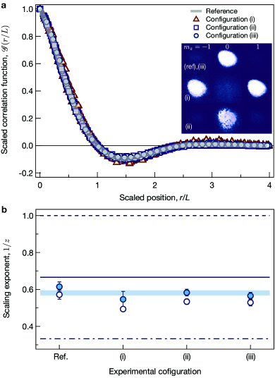
Figure 4: Universal coarsening dynamics in the easy-axis ferromagnetic phase. a, Scaled spin correlation functions $\mathcal{G}(r/L)$ in the coarsening stage regarding four different experimental configurations (see main text). The reference experiment refers to the coarsening dynamics at $q_{\rm EA}/h=-200~{}\rm Hz$ with the polar phase as initial state (Fig. 2a.) The inset shows spin-resolved absorption images for the various initial conditions. The vortices in (ii) can be identified after 6 ms of short time-of-flight. b, Dynamical scaling exponents under various configurations. Data with closed (open) circles represent the exponent after (without) deconvolution. Error bars denote the fit errors (resampling error is smaller than the fit errors). The shaded line is the dynamic exponent obtained from our finite-sized simulations, and the solid line indicates the dynamic exponents for the inertial hydrodynamic regime in the thermodynamic limit $1/z=2/3$. The experimental results are distinguished from other dynamic exponents in a binary fluid universality class in the viscous $1/z=1$ (dashed line) and diffusive $1/z=1/3$ (dashed-dot lines) regimes.

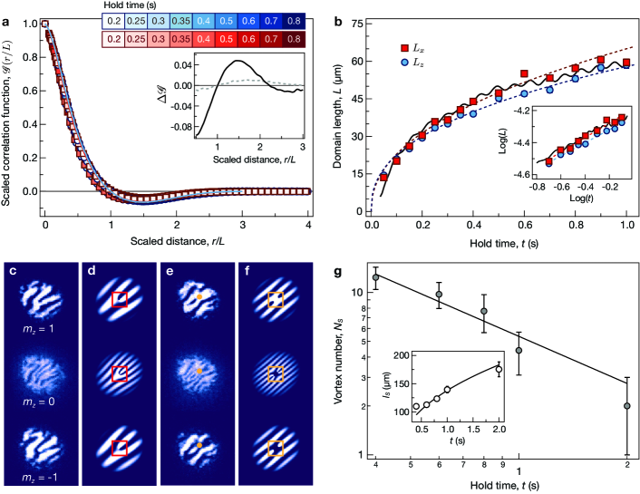
Figure 5: Coarsening dynamics in the isotropic ferromagnetic phase. a, Scaled correlation functions of magnetization along the $x$ (red square) and $z$ axes (blue circles) in the experiment as well as from theory (solid line). The domain length $L$ is characterized by the first-zero of the correlation function for both axes, $G_{x,z}(L,t)=0$. Inset: differences in scaled correlation functions. The solid line is $\Delta\mathcal{G}=\mathcal{G}_{q_{\rm Iso}}-\mathcal{G}_{q_{\rm EA}}$, where $\mathcal{G}_{q_{\rm Iso}}=(\mathcal{G}_{x}+\mathcal{G}_{z})/2$ and $\mathcal{G}_{q_{\rm EA}}$ are obtained from interpolating data in Fig. 2a. The dashed line is $\mathcal{G}_{x}-\mathcal{G}_{z}$. b, Growth dynamics of the spin domain in each axis. The solid line is the numerical result using our experimental parameters. The inset shows a log-log plot of the domain length dynamics, where we extract the scaling exponent by a linear fit (dashed lines). c, Matter-wave interference images during the coarsening dynamics ($t=1~{}\rm s$). The two-to-one (three-to-one) fork-shape fringes in the spin $\ket{\pm 1}$ ($\ket{0}$) state represent phase windings of $2\pi$ ($4\pi$) around the vortex core. d, Simulated interference pattern with a spin vortex at the trap center. e, Interference images with spin vortex and anti-vortex pairs at $t=1~{}\rm s$ (orange circle). f, Numerical simulations with the vortex pair located at the trap center ($H$-shaped pattern, orange box). g, Number of spin vortices $N_{S}$ as a function of time. Inset: the intervortex distance $l_{S}$ during time evolution. Solid lines are power-law guidelines, $N_{S}(t)\sim 1/L(t)^{2}$ and $l_{S}\sim L(t)$. The vortex number is the average over 40 independent experiments, and the error bars indicate 1 standard error of mean.

Figure 5 summarizes the experimental results on the coarsening dynamics under the spin isotropic Hamiltonian. Since the spin vectors can point in an arbitrary direction, domain coarsening is observed in both $M_{x}$ and $M_{z}$ [29]. Following the same analysis as in the easy-axis quench experiment, we rescale the correlation functions by $L(t)$ and observe their collapse into a single curve (Fig. 5a), in line with the mean-field analysis. The newly obtained universal curves are similar in each axis measurement but are distinctive from those of the easy-axis quench experiment (Fig. 5a inset), implying that the dynamics at the spin isotropic point belong to different universality classes. This can be further supported by the scaling exponent in the domain length $L(t)\sim t^{1/z}$ (Fig. 5b). We find the scaling exponents to be $1/z\simeq 0.45(3)$ for $M_{x}$ and $1/z\simeq 0.41(2)$ for $M_{z}$. Here, the exponents are close to the prediction $1/z=0.5$ and show good agreement with the finite size numerical simulations, $1/z_{\rm sim}\simeq 0.40(1)$.

To identify the underlying mechanism responsible for the coarsening dynamics in the SO(3) phase, we monitor the spin vortices and study their decay dynamics during the coarsening stage. For this reason, matter-wave inteferometry is adopted that can identify the position of the vortex cores by reading out the relative phase winding between spin states [29]. Fig. 5c shows interference patterns at $t=1$ s after quenching, where the fork-shaped fringes are well represented in all three spin components. We also observe images with closely bounded vortex and anti-vortex pairs (Fig. 5e). The existence of these spin vortices and vortex pairs is well reproduced in the simulated interference images (Fig. 5d,f).

Assigning the position of the spin vortex (vortex pairs) to the joint point in the fork-shaped ($H$-shaped) patterns, we count the spin vortex number $N_{S}$ and calculate the average distance between vortices $l_{S}$ at various hold times (Fig. 5g). The vortex number gradually decays, while the mean distance increases as time evolves. Since the imaging resolution is larger than the spin healing length, we underestimate the vortex number when the condensate contains many vortices. Nevertheless, the vortex number scales with the domain size, such that $N_{S}\sim 1/L(t)^{2}$ and $l_{S}\sim L(t)$. The decay process of spin vortex pairs occurs at a similar timescale [29], hinting to its intricate connection with the universal coarsening dynamics in the isotropic SO(3) symmetric phase. This is further supported from our numeric simulation, where we are able to calculate the argument of the transverse spin-vector and track the respective phase jumps [29].

In conclusion, we observe universal coarsening dynamics in two dimensions utilizing a strongly ferromagnetic spinor condensate. We find that the universal dynamics can be categorized into a well-defined universality class based on the symmetry of the order parameter and the dynamics of topological defects, such as domain walls and spin vortices. Our research demonstrates diverse capabilities of cold atom quantum simulators in characterizing nonequilibrium quantum dynamics, thus providing a steppingstone to a comprehensive understanding of quantum thermalization process in multidisciplinary research fields. Further extensions include the investigation of the universal dynamics mediated by other types of excitations, such as vortices in a two-dimensional superfluid [39, 14, 38], solitons in one dimension [23, 40], magnons in the Heisenberg spin model [41, 42], and chiral quantum magnetization with spin-orbit interaction [43, 44]. Moreover, our strongly interacting platform offers new opportunities to explore long-time thermalization dynamics in two dimensions, where the long-lived topological defects can slow down equilibration [45].

Supplementary Material for

Classifying the universal dynamics of a quenched ferromagnetic superfluid in two dimensions

I Experimental systems and data analysis

I.1 Experimental parameters

We create a spinor condensate of ⁷Li atoms in a quasi two-dimensional optical dipole trap [28], with frequencies $(\omega_{x},\omega_{y},\omega_{z})=2\pi\times(7,8,635)~{}\rm{Hz}$. The condensate contains $2.7\times 10^{6}$ atoms and has negligible thermal fraction ($<5\%$). The chemical potential of the condensate is $\mu/h=310~{}\rm{Hz}$, indicating that transversal excitations are suppressed and our system is in two dimensions. To prepare the condensate in the polar phase, an external magnetic field of $B=1$ G is applied along the vertical axis. Under this magnetic field, the quadratic Zeeman energy (QZE) is larger than the critical point $q>q_{c}=2\absolutevalue{c}$ (Fig. 1a in the main text) so that all atoms populate the same spin state $\ket{F=1,m_{z}=0}\equiv\ket{1,0}$.

I.2 Quenching protocols

Instantaneous quenching of QZE is experimentally realized with the aid of the microwave dressing technique [34]. The QZE is given by $q=q_{\rm B}+q_{\rm MW}$, where $q_{\rm B}/h=610~{}{\rm Hz/(G^{2}B^{2})}$ is the second-order Zeeman splitting of the hypefine states of ⁷Li atoms, and $q_{\rm MW}/h=\Omega^{2}/4\delta$ denotes the respective energy shift due to the microwave field. In the experiment, we ramp down the external bias field to $B\simeq 100~{}\rm mG$ in 7 ms and simultaneously tune the microwave frequency, such that the QZE value is always larger than the critical point ($q>q_{c}$) during the field ramp. We initiate the nonequilibrium dynamics of the spinor gas by changing the microwave frequency within $1~{}\mu{}\rm s$ and quench the QZE to a target point. The field gradient is compensated to below $30~{}\mu{}\rm G/cm$ so that we observe randomly oriented domain walls even a long time after the quench ($t=2$ s).

Long-term drifts in the experimental parameters are calibrated by taking reference images. For example, the average magnetization at $t=2$ s is monitored every 150 min (corresponding to approximately 300 measurements), and we adjust the field gradient if needed. The uncertainty of the QZE is mostly due to the external field noise, which is $\pm 0.3~{}{\rm Hz}$. The small fluctuations in the QZE are negligible even for the spin isotropic coarsening dynamics within the considered time scales. The small but nonzero QZE could lead to a coarsening transition at longer evolution times, where the scaling exponents of the domain lengths follow the easy-plane or easy-axis phase dynamics [27]. The field fluctuations in the experiment are $q/q_{0}<10^{-3}$ so that the transition occurs after $t>1~{}{\rm s}~{}(t>2,000~{}t_{s})$.

I.3 In-situ spin-resolved Imaging

Atomic density distributions in the lower hyperfine spin states are recorded using the standard absorption imaging technique after selectively converting a target spin state into an upper hyperfine state. Under the magnetic field of 100 mG, for instance, we apply a microwave that transfers the atoms from the $\ket{1,1}$ to the $\ket{2,1}$ state. The atomic distribution in the $\ket{2,1}$ state is subsequently imaged by a resonant light with $\ket{F=2}\rightarrow\ket{F^{\prime}=3}$ transition. The atoms in the other spin states are measured in a similar manner. Namely, after taking the first image, we apply an additional microwave pulse, flipping the hyperfine spin states from $\ket{1,0}$ ($\ket{1,-1}$) to $\ket{2,1}$ ($\ket{2,-2}$), and imaging the transferred atoms. To avoid cross-talk between images in the $F=1$ state, we remove all atoms in the $\ket{F=2}$ state before taking subsequent images. This imaging sequence is also used to measure the magnetization along the spin $x$ direction, $M_{x}$. Indeed, by applying a resonant radio-frequency pulse, we rotate the measurement basis from the spin $z$ axis to the $x$ axis and record the density distribution of each spin state. Paradigmatic images of magnetization along $x$ and $z$ following a quench to the spin isotropic point are shown in Fig. S1.

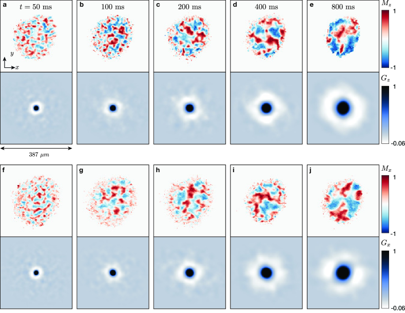
Figure S1: Time evolution of spin domains in the isotropic ferromagnetic phase. a-e, Longitudinal magnetization $M_{z}$ (upper) and its two-dimensional spin correlation functions $G_{z}(x,y)$ (below) at various hold times. f-j, Snapshots of transverse magnetization $M_{x}$ and the correlation functions $G_{x}(x,y)$. In contrast to the easy-axis phase, in the spin isotropic point, coarsening dynamics are observed in both axes, and the domain boundaries are much broader than those of the $q<0$ spin domains. The spin correlation functions are averaged over 100 different realizations at a given hold time.

To characterize the imaging resolution, we prepare a spin spiral structure, which displays periodic density modulation in each spin state. This state can be created by evolving the spin vector in the horizontal plane under a finite field gradient [46]. The modulation period $\lambda_{\rm sp}$ is determined by the gradient strength and exposure time, where the modulation contrast is affected by our imaging system. For example, the contrast drops to $30\%$ at $\lambda_{\rm sp}=10~{}\mu{}\rm m$. By investigating the dependence of the contrast on the wavelength $\lambda_{\rm sp}$, we estimate that the imaging resolution is $5~{}\mu{}\rm m$. The imaging parameters are optimized to have a better signal-to-noise ratio and imaging resolution. We set the imaging light intensity to $0.5~{}I_{\rm sat}$ and the imaging pulse to $4~{}\mu{}\rm s$, where $I_{\rm sat}=2.5~{}\rm mW/cm^{2}$ is the saturation intensity.

I.4 Time interval of the universal regime

To extract the dynamical scaling exponents, we set the time interval for the universal dynamics as $t\in[0.2~{}{\rm~{}s},0.8{\rm~{}s}]$. The upper bound of the considered time window is limited by the finite size of the system and finite lifetime of the condensate. Due to the finite trap volume, only 2-3 domains are left after 1 s (Fig. S2b). Also, the coarsening dynamics slows down when the domain length is comparable to the condensate Thomas-Fermi radius, $R_{\rm TF}\simeq 90~{}\mu{}m$. Moreover, under the microwave dressing field, we observe a gradual decay of the domain length $L(t)\propto e^{-t/\tau}$ with decay constant $\tau=7$ s. To minimize the suppression of the domain growth, we set $t_{U}=0.8$ s as the upper limit for the scaling regime.

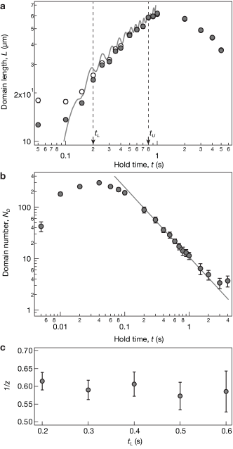
Figure S2: Full time evolution of coarsening dynamics and scaling exponents in the easy-axis ferromagnetic phase. a, Domain length $L(t)$ in the full time evolution accessible during the experiment. Closed (open) circles represent the domain length after (without) deconvolution. Dashed lines represent the scaling time interval $t\in[0.2~{}\rm s,0.8~{}\rm s]$. b, Number of magnetic domains after the quench. The domain numbers $N_{D}$ is counted by using the Hoshen-Koppelman algorithm. The domain number follows the power law decay (solid line), $N_{D}\sim t^{-2/z}$ with $1/z=0.63(4)$. c, Dependence of the scaling exponents $1/z$ on the lower bound for the time interval $t_{L}$. The error bars indicate the 1$\sigma$ confidence interval of the fit parameters.

The lower bound of the time interval is chosen to be $t_{L}=0.2~{}\rm s$ since it ensures that the condensate enters into the coarsening stage after the quench. Before the initiation of the coarsening stage, we observe a rapid increase of the magnetic domain number (Fig. S2b). The maximum domain number takes place around $t\sim 50~{}\rm ms$, and subsequently reduces due to merging while the most prominent decay occurs after $t\sim 100~{}\rm ms$. The coarsening dynamics begins afterwards where the domain length increases due to merging of the domain walls, and the correlation function starts to follow the universal curve, see e.g. Fig. 2a and 4a in the main text. We consider $t_{L}\geq 0.2~{}\rm s$ ensuring that we are away from the early stage of the coarsening and also the domain length is much larger than the spin healing length [31]. The robustness of the dynamical scaling exponent is shown in the Fig. S2c. The scaling exponent is also manifested on the domain number $N_{D}$ after the quench (Fig. S2b). In the universal time interval, the domain number simply follows the power law $N_{D}\sim 1/L^{2}(t)\sim t^{-2/z}$, where we find a consistent dynamic scaling exponent of $1/z=0.63(4)$.

I.5 Vortex shedding in the polar condensate

To demonstrate the insensitivity of the dynamical exponent on the initial conditions, we imprint many vortices in the polar phase before the quench. An initial state containing many vortices can be prepared by adopting the vortex shedding technique [47, 48]. Specifically, a repulsive optical barrier is imposed at the trap center and is translated by a piezo mirror mount. When the speed of the barrier exceeds a critical threshold, vortices and anti-vortices are nucleated in the condensate [47]. The optical obstacle is made of focused, blue-detuned laser light of $532~{}\textrm{nm}$ along the $z$-direction. Its $1/e^{2}$ beam waist is $8~{}\mu\rm m$ and the obstacle height is $V_{0}/\mu\approx 3$. The sweeping distance of the barrier from the trap center is $d=60~{}\mu\rm m$ and its translation speed is 6 mm/s. The vortex cores can be identified after 6 ms of time-of-flight (inset of Fig. 4), and in particular around 15 vortices are nucleated before the quench. Indeed, using this initial state containing vortices we performed the quench dynamics as described above and measured the critical exponent which remained unaffected.

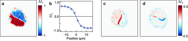
Figure S3: Magnetic domain wall in the easy-axis ferromagnetic phase. a, Magnetization $M_{z}$ after 1.5 s of hold time, and b, the cross-section profile at the domain wall boundary. The solid line is a fit curve $M_{z}(r)=M_{z0}\tanh(r/\xi_{d})$ with $\xi_{d}=4.5(2)~{}\mu{}m$. c,d, Magnetization along the horizontal axis $M_{x}$. The spin vectors could be aligned on the same axis (c, Bloch or Neel-type domain wall) or point in opposite directions (d, Bloch line). A long wavelength modulation of the horizontal spin vector could imply the presence of spin wave excitations in the magnetic domain.

II Topological defects

II.1 Domain walls

The coarsening dynamics in the easy-axis phase is driven by the motion of magnetic domains. Since the order parameter possess $\mathbb{Z}_{2}$ spin symmetry, the domain walls between the $\ket{\pm 1}$ states have sharp edges, which can be identified by examining the spin vector in the $x$ and $z$ directions (Fig. S3). Upon analysis, it is found that the domain walls exhibit Neel-type or Bloch-type characteristics with a long-wavelength modulation in the transverse magnetization $M_{z}$. This behavior is indicative of magnon excitations or spin waves, in which oppositely charged Bloch lines are annihilated during the coarsening process [49].

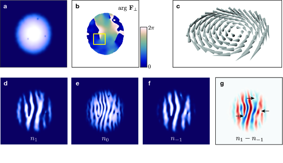
Figure S4: Numeric simulations of the matter-wave interference for the $\mathbb{Z}_{2}$ spin vortices. a, Density profile and b, in-plane spin vector after $t=3.5~{}\rm s$ of domain coarsening dynamics at the spin isotropic point. c, Spin texture near the highlighted region (yellow box). Not only the in-plane spin vector, but also the longitudinal spin vector turn around the vortex core. d-f, Simulated images after the matter-wave interference. Fork-shaped patterns are well identified in all spin components. g, The spin imbalance image, and the vortex positions are marked by arrows. The positions of the spin vortices are well identified.

II.2 Spin vortices

The spin components $(\zeta_{1},\zeta_{0},\zeta_{-1})^{T}$ of the $\mathbb{Z}_{2}$ vortex [50] can be written as,

$$\zeta_{sv}(\mathbf{r})=\left(\begin{array}[]{c}e^{-i\phi(\mathbf{r})}\cos^{2}\frac{\theta(\mathbf{r})}{2}\\ \frac{1}{\sqrt{2}}\sin\theta(\mathbf{r})\\ e^{i\phi(\mathbf{r})}\sin^{2}\frac{\theta(\mathbf{r})}{2}\end{array}\right),$$ (S1)

where $(\theta,\phi)$ denote the polar and azimuthal angles of the spin vector respectively, and $\mathbf{r}=(x,y,z)$. Since the winding number in each spin component is different, one can infer the existence of the spin vortex by measuring the relative phase between them [51, 52]. For example, interfering the spin $\ket{1,1}$ and $\ket{1,-1}$ states reveals a 4$\pi$ phase winding around the vortex core. Similarly, the spin $\ket{1,0}$ and spin $\ket{1,\pm{1}}$ states can interfere to display 2$\pi$ phase windings around the generated vortices. To realize the matter-wave interference, we perform the following experimental procedure: A field gradient of $60~{}\textrm{mG/cm}$ is applied to the condensate for $t_{\rm grad}=6$ ms. Next, a resonant radio-frequency pulse is employed in order to induce the $\ket{1,0}\leftrightarrow\ket{1,\pm 1}$ transition. Finally, we image all spin components in the $F=1$ state using the selective spin transfer imaging technique.

In the vortex-free state, we observe stripe lines along the gradient direction as a result of the phase accumulation across the condensate. With the phase defect, however, the stripe lines are dislocated, where we can read out the magnitude of the relative phase winding in the spin texture. Because of our finite imaging resolution, we set the periodicity of the stripe patterns to be $\sim 10~{}\mu{}m$. Accordingly, this becomes the minimum distance between spin vortices detected with this scheme. To validate the vortex identification protocol, we consider reference data from our numerical simulations where $\mathbb{Z}_{2}$ spin vortices occur during the coarsening dynamics at $q_{\rm Iso}/h=0~{}\rm{Hz}$ (Fig. S4). The vortex positions in the numerical simulations, as determined by analyzing the spin vector, are the same as the phase singular points that were identified using the matter-wave interference technique.

III Theoretical methodology

III.1 Mean-field equations of the spin-1 gas

The dynamics of the spin-1 condensate is described by the following set of coupled 3D Gross-Pitaevskii equations of motion

$$\frac{\partial{\Psi(\mathbf{r};t)}}{\partial t}=-\frac{\hslash^{2}\nabla^{2}}{2M}+V_{\rm trap}(\mathbf{r})+qf^{2}_{z}+c_{0}n(\mathbf{r};t)+c_{1}\mathbf{F}(\mathbf{r};t)\cdot\mathbf{f}.$$ (S2)

The wave function of each hyperfine $m_{F}=-1,0,1$ level is denoted by $\Psi=({\Psi}_{1},{\Psi}_{0},{\Psi}_{-1})^{T}$, the atom mass is $\rm M$ and $\mathbf{r}\equiv\{x,y,z\}$. The spin-independent non-linear term, $c_{0}n$, is characterized by the effective strength, $c_{0}=4\pi\hbar^{2}(a_{0}+a_{2})/(3\rm M)$, and total density, $n=\sum_{m_{F}}\absolutevalue{\Psi_{m_{F}}}^{2}$. Here, $a_{0}$ and $a_{2}$ refer to the 3D $s$-wave scattering lengths of the atoms in the scattering channels with total spin $F=0$ and $F=2$ respectively. In contrast, the spin-dependent nonlinear term $c_{2}=\mathbf{F}\cdot\mathbf{f}$ accounting for interactions among the hyperfine levels contains the coupling constant $c_{2}=4\pi\hbar^{2}(a_{2}-a_{0})/(3\rm M)$ and spin density $\mathbf{F}=(F_{x},F_{y},F_{z})$ whose $j=\{x,y,z\}$ component is $F_{j}=\Psi_{m_{F}}^{\dagger}f_{j}\Psi_{m_{F}}$ and $f_{j}$ denote the spin-1 matrices. As discussed in the main text we focus on the $\rm{}^{7}Li$ condensate possessing strong ferromagnetic interactions, i.e. $c_{2}<0$. The 3D external harmonic confinement $V_{\rm trap}=\frac{1}{2}M(\omega_{x}^{2}x^{2}+\omega_{y}^{2}y^{2}+\omega^{2}_{z}z^{2})$ is characterized by the in-plane trap frequency $\omega_{x}\approx\omega_{y}$ and the out-of-plane one $\omega_{z}$ obeying the condition $\omega_{z}\gg\omega_{x}\approx\omega_{y}$ which restricts the atomic motion in 2D. Throughout, we consider the experimentally used trap frequencies $(\omega_{x},\omega_{y},\omega_{z})=2\pi\times(7,8,635)~{}\rm Hz$. Moreover, the length and energy scales of the system are expressed in terms of the harmonic oscillator length $l_{\rm osc}=\sqrt{\hslash/M\omega_{x}}$ and the energy quanta $\hslash\omega$. For convenience of our simulations we further cast the 3D GP Eq. (S2) into a dimensionless form by rescaling the spatial coordinates as $x^{\prime}=x/l_{osc}$, $y^{\prime}=y/l_{osc}$ and $z^{\prime}=z/l_{osc}$, the time as $t^{\prime}=\omega_{x}t$ and the wavefunction as $\Psi_{m_{F}}(x^{\prime},y^{\prime},z^{\prime})=\sqrt{(l^{3}_{osc}/N)}\Psi_{m_{F}}(x,y,z)$, see e.g. Ref. [53, 54] for further details.

Depending on the relative strength of $q/(|c_{2}|n)$ it is possible to realize a rich phase diagram containing first and second-order phase transitions as described in Ref. [33]. For instance, the quantum critical point $q=q_{c}=2\absolutevalue{c_{2}}n_{\rm peak}$, with $n_{\rm peak}$ being the condensate peak density around the trap center, separates the so-called unmagnetized polar state where all atoms are in the $m_{F}=0$ state from the easy-plane ferromagnetic phase with all $m_{F}$ states being occupied. The latter phase occurs within the interval $0<q<q_{c}$ and it is characterized by the order parameter $\mathbf{F_{\perp}}=F_{x}+iF_{y}$ referring to the transverse magnetization [27] where $F_{x}=[\psi^{*}_{1}\psi_{0}+\psi^{*}_{0}(\psi_{1}+\psi_{-1})+\psi^{*}_{-1}\psi_{0}]/\sqrt{2}$ and $F_{y}=i[-\psi^{*}_{1}\psi_{0}+\psi^{*}_{0}(\psi_{1}-\psi_{-1})+\psi^{*}_{-1}\psi_{0}]/\sqrt{2}$. On the other hand, for $q<0$ the ground state corresponds to an easy-axis ferromagnetic phase where the magnetization lies along the $z$-axis and the relevant order parameter is the longitudinal magnetization $\mathbf{F}_{z}=\absolutevalue{\Psi_{+1}}^{2}-\absolutevalue{\Psi_{-1}}^{2}$.

III.2 Initial state preparation using quantum and thermal fluctuations

The initial state of the spin-1 gas (the easy-axis polar state) is realized at $q=2q_{c}$, with the critical quadratic Zeeman shift $q_{c}=2|c_{2}|n_{\rm peak}/h$. It is represented by the wave function

$$\Psi_{\rm polar}=(0,{\Psi}_{0},0)^{T}.$$ (S3)

The latter is determined by numerically solving Eq. (S2) using the split-time Crank-Nicholson method in imaginary time [55, 56]. In order to trigger the dynamics, we perform a sudden change of the quadratic zeeman coefficient $q$ from its initial value $q_{i}/h=510~{}\rm Hz$ (polar state) to a final value $q_{\rm EA}/h=-200~{}\rm Hz$ (easy-axis state) or $q_{\rm Iso}/h=0$ (isotropic point).

To monitor the system’s nonequilibrium dynamics, it is essential to consider the presence of quantum and thermal fluctuations on top of the initial zero temperature mean-field state [Eq. (S3)]. This contribution seeds the ensuing dynamical instabilities occurring once $q$ is quenched. We incorporate the impact of quantum and thermal effects exploiting the truncated Wigner approximation [32], namely express the wave function as $\bm{\Psi}_{I}=\bm{\Psi_{\rm polar}}+\bm{\delta}$, where $\bm{\delta}=(\delta^{+1},\delta^{0},\delta^{-1})^{T}$ is a noise vector constructed using the Bogoliubov quasi-particle modes of the system. Specifically, first we calculate the steady state solution ($\Psi_{{\rm polar}}$), which is subsequently perturbed according to the following ansatz $\Psi_{m_{F}}=\Psi_{{\rm polar}}+\epsilon\big{(}U_{m_{F}}e^{i\Omega t}+V^{*}_{m_{F}}e^{-i\Omega^{*}t}\big{)}$. Inserting this ansatz into Eq. (S2) and linearizing with respect to the small amplitude $\epsilon$ leads to the corresponding energy eigenvalue problem which is numerically solved through diagonalization allowing us to determine the underlying eigenfrequencies $\{\Omega^{j}\}$ and eigenfunctions $\{U^{j}_{m_{F}},V^{j}_{m_{F}}\}$. For the polar steady state, where $\Psi_{\pm 1}=0$ and $\Psi_{0}=\Psi_{0}$, the respective eigenvalue problem reads

$$\begin{pmatrix}U_{0}\\ V_{0}\\ U_{1}\\ V_{1}\\ U_{-1}\\ V_{-1}\end{pmatrix}\begin{pmatrix}a&b&0&0&0&0\\ -b^{*}&-a&0&0&0&0\\ 0&0&c&0&0&d\\ 0&0&0&-c&-d^{*}&0\\ 0&0&0&d&c&0\\ 0&0&-d^{*}&0&0&-c\\ \end{pmatrix}=\Omega\begin{pmatrix}U_{0}\\ V_{0}\\ U_{1}\\ V_{1}\\ U_{-1}\\ V_{-1}.\end{pmatrix}$$ (S4)

Here, the matrix elements are given by $a=-\frac{1}{2}\nabla^{2}_{\perp}+V-\mu+2c_{0}\absolutevalue{\Psi_{0}}^{2}$, $b=c_{0}(\Psi_{0})^{2}$, $c=-\frac{1}{2}\nabla^{2}_{\perp}+V_{{\rm trap}}-\mu+q$ and $d=c_{2}(\Psi_{0})^{2}$ with $\mu$ being the system’s chemical potential. Having at hand the eigenmodes $\{U^{j}_{m_{F}},V^{j}_{m_{F}}\}$ and eigenvalues $\Omega^{j}$, it is possible to express the noise field in the form $\delta_{m_{F}}=\sum_{j>0}U^{j}_{m_{F}}\beta^{j}_{m_{F}}+(V^{j}_{m_{F}})^{*}(\beta^{j}_{m_{F}})^{*}$, i.e. decomposing it in terms of the low-lying collective modes of the initial state which are weighted by the random valued coefficients $\beta^{j}_{m_{F}}$. These coefficients are generated as

$$\beta^{j}_{m_{F}=\pm 1}=\frac{x_{j}+iy_{j}}{2}~{}~{}~{}\textrm{and}~{}~{}~{}\beta^{j}_{m_{F}=0}=\sqrt{(\bar{n}_{j}+\frac{1}{2})}\frac{x_{j}+iy_{j}}{\sqrt{2}},$$ (S5)

where $x_{j}$ and $y_{j}$ are random values taken from a normally distributed Gaussian distribution characterized by zero mean and unit variance, while $\bar{n}_{j}=(e^{\Omega^{j}\hbar/(K_{B}T)}-1)^{-1}$ denotes the mean thermal occupation of BEC at temperature $T$. Notice also that the constant $1/2$ factor appearing in Eq. (S5) stems from the vacuum noise. In this sense, the initial state of the system comprises of a condensate with thermal excitations in the $m_{F}=0$ and only vacuum noise in the $m_{F}=\pm 1$ components.

In order to render the observables of interest independent of the presence of the above-discussed noise terms we employ multiple realizations, e.g. for a specific quench, and afterwards perform an averaging. Typical samples leading to a converged behavior of the observables consist of 500 different realizations.

III.3 Generation of topological defects and coarsening stage

Let us visualize the individual stages of the universal dynamics upon quenching the quadratic Zeeman coefficient $q$ from the polar to the easy-axis phase of the trapped ⁷Li spinor BEC with $N=3\times 10^{6}$ atoms, including the spontaneous nucleation of topological defects and the coarsening. Recall that while the system is initialized in a polar state at $q_{i}/h=510~{}\rm Hz$ where only the $m_{F}=0$ component is occupied we consider the presence of thermal excitations (see the previous section) to trigger spin-mixing dynamics.

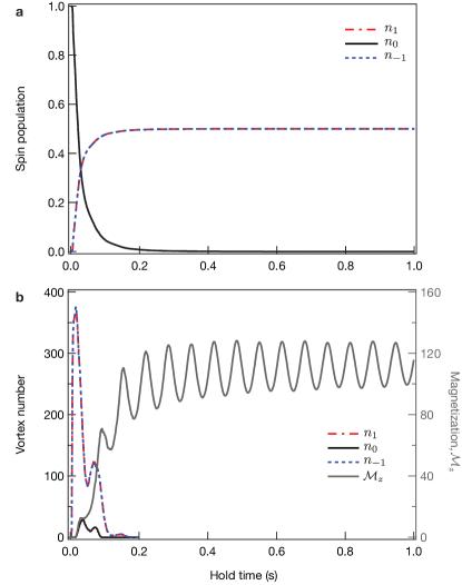
Figure S5: a, Time-evolution of the normalized particle number $n_{m_{F}}=N_{m_{F}}(t)/N$ of each hyperfine state (see legend) showing the quench-induced spin-mixing process. b, Dynamics of the number of gauge vortices, $N_{G}$, (left axis) of each spin component (see legend) and the second moment of the magnetization $\mathcal{M}_{z}(t)$ (right axis). The rise of $N_{G}$ at $0<t<40\rm ms$ justifies vortex nucleation in the bulk, while its subsequent decrease is related with vortex annihilation and entrance to the coarsening state. The finite $\mathcal{M}_{z}(t)$ explicates the emergence of domains among $m_{F}=\pm 1$ states, while its oscillatory behavior is caused by the trap.

After the quench, the polar state becomes unstable transitioning towards the easy-axis phase and thus featuring particle transfer from the $m_{F}=0$ to the $m_{F}=\pm 1$ states as shown in Fig. S5a. Indeed, a ballistic rise of the population $N_{\pm 1}(t)$ of the $m_{F}=\pm 1$ components is observed at the early stages of the dynamics $0<t<50$ ms, which saturates to $N_{\pm}=0.5N$ for $t>100$ ms. This dynamical crossing of the relevant first-order phase transition results in the spontaneous symmetry breaking of $\mathbb{Z}_{2}$ symmetry manifesting by the generation of topological defects. The latter refer here to a complex network of gauge vortices and anti-vortices in all components; see, for instance, the snapshots of the component densities $n_{m_{F}}(\mathbf{r})$, and their respective phase profiles $\Phi_{m_{F}}(\mathbf{r})$ depicted in Fig. S6.

The production of gauge vortices and antivortices in the course of the time-evolution is further confirmed by tracking the phase winding of the wave function of each component and thus identifying the underlying vortex number $N_{G}$. $N_{G}$ is presented in Fig. S5b and provides an estimate for the overall vortical content of the system. Indeed, the sharp increasing trend of $N_{G}$ reflects the rapid production of vortices and anti-vortices in the system within $0<t<15~{}\rm ms$. Afterwards, it declines as the vortices and antivortices start to annihilate or drift out of the spinor BEC.

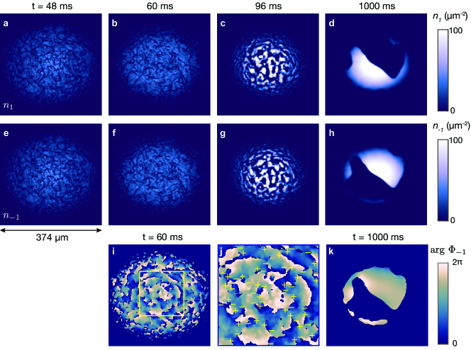
Figure S6: Density profile of the spin $m_{F}=1$ component a-d, and $m_{F}=-1$ component e-h, in the easy-axis quench at various hold time (legends). i,j, In the early time after the quench, gauge vortices are nucleated (yellow markers $\pm 1$ refers to the vorticity). After the vortex annihilation, the magnetic domains are formed, entering into the universal coarsening stage. k, The gauge vortices are not observed in the magnetic domains.

Consequently, as time evolves, the number of vortical defects drops and the build-up of magnetic domains among the $m_{F}=\pm 1$ components occurs (Fig. S6c,g), where the spinor system starts to exhibit a universal scaling exponent in the growth of correlation length. The formation of these magnetic domains becomes evident by inspecting the fluctuation of the axial magnetization, $F_{z}(\mathbf{r})=\absolutevalue{\Psi_{1}(\mathbf{r})}^{2}-\absolutevalue{\Psi_{-1}(\mathbf{r})}^{2}$, through $\mathcal{M}_{z}(t)=\int d\mathbf{r}=[\innerproduct{F_{z}^{2}(t)}{F_{z}^{2}(t)}-\innerproduct{F_{z}(t)}{F_{z}(t)}^{2}]/n^{2}_{\rm peak}=F^{2}_{z}(\mathbf{r})/n^{2}_{{\rm peak}}$ depicted in Fig. S5b. The oscillatory behavior of $\mathcal{M}_{z}(t)$ (around a mean value) reflects the background breathing motion with frequency $\omega_{br}\approx 2\pi\times 16~{}\rm Hz$. It is thus a trap effect and will disappear in its absence [31]. Since, in a quasi-2D system, vortex patterns are point-like defects, whereas magnetic domain walls refer to linear topological defects we indeed observe a transition from point to linear topological defect formation in the course of the evolution, see Figs. S6a-c and Figs. S6e-g. In fact, these linear defects gradually merge and play the dominant role in the late time universal dynamics. Specifically, their merging eventually leads to the creation of a single domain wall which is persistent for an extended period of time (Fig. S6d, h).

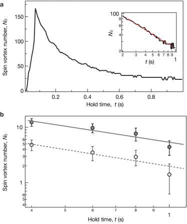
Figure S7: a, Spin vortices number $N_{S}$ as a function of hold time after quenching the quadratic Zeeman energy to $q_{\rm Iso}=0$. Inset: log-log plot of the $N_{S}$ during the coarsening stage. The vortex number follows a power law decay $N_{S}\sim t^{-2/z}$ with $1/z=0.43(1)$. b, Decay dynamics of vortices (closed circle) and vortex pairs (open circle) in the experiment. The solid lines are the power law fit $t^{-2/z}$ to data, where it shows $1/z=0.48(8)$ for the total vortex (closed circle) and $1/z=0.5(1)$ for vortex dipole (open circle).

Next, we turn our attention to the quench in the isotropic phase, $q_{Iso}=0$, where spin vortices are generated in the short time dynamics as argued in the main text. To monitor the number of spin vortices in the course of the evolution, we determine the transverse spin component, $\mathbf{F}{{}_{\perp}}=(F_{x},F_{y})$, and subsequently calculate its argument $\phi=\tan^{-1}(F_{y}/F_{x})$ in the $x$-$y$ plane. We detect the respective phase jumps using $\oint_{C}d\phi=2\pi n_{\phi}$, where $\mathit{C}$ denotes a closed contour around a target location. The spin vortices are identified in the location where $n_{\phi}=\pm 1$ indicating spin vortices and anti-vortices respectively. The time evolution of the spin-vortex number, $N_{s}$, obtained through our numerical calculations is demonstrated in Fig. S7a. Following an initial sharp rise, the spin vortices begin to decay as the coarsening dynamics commences and the magnetic domain length grows. Remarkably, the decay of spin vortices obeys the power law $N_{s}\approx t^{-2/z}$, where $1/z=0.43(1)$ represents the critical exponent which is in accordance with the experimental observations.

In Fig. S7b, we present our experimental observations of the time evolution of spin vortex number. The decay of the total spin vortex number is found to follow a power law, with an exponent of $1/z=0.48(8)$, while the decay of the spin voprtex anti-vortex pairs satisfies a power law with an exponent of $1/z=0.5(1)$. It is worth noting that the vortex number is found to be relatively lower in the experiment than in the simulations due to the finite imaging resolution. Nevertheless, our investigation on the dynamics of spin-vortices and their power law decay sheds light on the non-linear defect formation and its relationship with the critical exponent, demonstrating excellent agreement between theory and experiment in substantiating the universal nature of the dynamics.

References

- Wilson [1975] K. G. Wilson, The renormalization group: Critical phenomena and the Kondo problem, Rev. Mod. Phys. 47, 773 (1975).
- Kadanoff [1990] L. P. Kadanoff, Scaling and universality in statistical physics, Physica A: Statistical Mechanics and its Applications 163, 1 (1990).
- Hohenberg and Halperin [1977] P. C. Hohenberg and B. I. Halperin, Theory of dynamic critical phenomena, Rev. Mod. Phys. 49, 435 (1977).
- Donner et al. [2007] T. Donner, S. Ritter, T. Bourdel, A. Öttl, M. Köhl, and T. Esslinger, Critical Behavior of a Trapped Interacting Bose Gas, Science 315, 1556 (2007).
- Polkovnikov et al. [2011] A. Polkovnikov, K. Sengupta, A. Silva, and M. Vengalattore, Colloquium: Nonequilibrium dynamics of closed interacting quantum systems, Rev. Mod. Phys. 83, 863 (2011).
- Eisert et al. [2015] J. Eisert, M. Friesdorf, and C. Gogolin, Quantum many-body systems out of equilibrium, Nat. Phys. 11, 123 (2015).
- Ueda [2020] M. Ueda, Quantum equilibration, thermalization and prethermalization in ultracold atoms, Nat. Rev. Phys. 2, 669 (2020).
- Bray [1994] A. Bray, Theory of phase-ordering kinetics, Advances in Physics 43, 357 (1994).
- Makotyn et al. [2014] P. Makotyn, C. E. Klauss, D. L. Goldberger, E. A. Cornell, and D. S. Jin, Universal dynamics of a degenerate unitary Bose gas, Nat. Phys. 10, 116 (2014).
- Eigen et al. [2018] C. Eigen, J. A. P. Glidden, R. Lopes, E. A. Cornell, R. P. Smith, and Z. Hadzibabic, Universal dynamics in an isolated one-dimensional Bose gas far from equilibrium, Nature (London) 563, 221 (2018).
- Prüfer et al. [2018] M. Prüfer, P. Kunkel, H. Strobel, S. Lannig, D. Linnemann, C.-M. Schmied, J. Berges, T. Gasenzer, and M. K. Oberthaler, Observation of universal dynamics in a spinor Bose gas far from equilibrium, Nature (London) 563, 217 (2018).
- Erne et al. [2018] S. Erne, R. Bücker, T. Gasenzer, J. Berges, and J. Schmiedmayer, Universal dynamics in an isolated one-dimensional Bose gas far from equilibrium, Nature (London) 563, 225 (2018).
- Glidden et al. [2021] J. A. P. Glidden, C. Eigen, L. H. Dogra, T. A. Hilker, R. P. Smith, and Z. Hadzibabic, Soliton-like magnetic domain wall motion induced by the interfacial Dzyaloshinskii–Moriya interaction, Nat. Phys. 17, 457 (2021).
- Johnstone et al. [2019] S. P. Johnstone, A. J. Groszek, P. T. Starkey, C. J. Billington, T. P. Simula, and K. Helmerson, Order from chaos: Observation of large-scale flow from turbulence in a two-dimensional superfluid, Science 364, 1267 (2019).
- Wei et al. [2022] D. Wei, A. Rubio-Abadal, B. Ye, F. Machado, J. Kemp, K. Srakaew, S. Hollerith, J. Rui, S. Gopalakrishnan, N. Y. Yao, I. Bloch, and J. Zeiher, Quantum simulations with ultracold atoms in optical lattices, Science 376, 716 (2022).
- Berges et al. [2008] J. Berges, A. Rothkopf, and J. Schmidt, Nonthermal Fixed Points: Effective Weak Coupling for Strongly Correlated Systems Far from Equilibrium, Phys. Rev. Lett. 101, 041603 (2008).
- Schole et al. [2012] J. Schole, B. Nowak, and T. Gasenzer, Critical dynamics of a two-dimensional superfluid near a nonthermal fixed point, Phys. Rev. A 86, 013624 (2012).
- Schmidt et al. [2012] M. Schmidt, S. Erne, B. Nowak, D. Sexty, and T. Gasenzer, Non-thermal fixed points and solitons in a one-dimensional Bose gas, New J. Phys. 14, 075005 (2012).
- Berges et al. [2014] J. Berges, K. Boguslavski, S. Schlichting, and R. Venugopalan, Turbulent thermalization process in heavy-ion collisions at ultrarelativistic energies, Phys. Rev. D 89, 074011 (2014).
- Berges et al. [2015] J. Berges, K. Boguslavski, S. Schlichting, and R. Venugopalan, Universality Far from Equilibrium: From Superfluid Bose Gases to Heavy-Ion Collisions, Phys. Rev. Lett. 114, 061601 (2015).
- Piñeiro Orioli et al. [2015] A. Piñeiro Orioli, K. Boguslavski, and J. Berges, Universal self-similar dynamics of relativistic and nonrelativistic field theories near nonthermal fixed points, Phys. Rev. D 92, 025041 (2015).
- Chantesana et al. [2019] I. Chantesana, A. Piñeiro Orioli, and T. Gasenzer, Kinetic theory of nonthermal fixed points in a Bose gas, Phys. Rev. A 99, 043620 (2019).
- Schmied et al. [2019] C.-M. Schmied, M. Prüfer, M. K. Oberthaler, and T. Gasenzer, Bidirectional universal dynamics in a spinor Bose gas close to a nonthermal fixed point, Phys. Rev. A 99, 033611 (2019).
- Mikheev et al. [2019] A. N. Mikheev, C.-M. Schmied, and T. Gasenzer, Low-energy effective theory of nonthermal fixed points in a multicomponent Bose gas, Phys. Rev. A 99, 063622 (2019).
- Kudo and Kawaguchi [2013] K. Kudo and Y. Kawaguchi, Magnetic domain growth in a ferromagnetic Bose-Einstein condensate: Effects of current, Phys. Rev. A 88, 013630 (2013).
- Williamson and Blakie [2016] L. A. Williamson and P. B. Blakie, Universal Coarsening Dynamics of a Quenched Ferromagnetic Spin-1 Condensate, Phys. Rev. Lett. 116, 025301 (2016).
- Williamson and Blakie [2017] L. A. Williamson and P. B. Blakie, Coarsening Dynamics of an Isotropic Ferromagnetic Superfluid, Phys. Rev. Lett. 119, 255301 (2017).
- Huh et al. [2020] S. Huh, K. Kim, K. Kwon, and J.-y. Choi, Observation of a strongly ferromagnetic spinor Bose-Einstein condensate, Phys. Rev. Research 2, 033471 (2020).
- [29] Materials and methods are available as supplementary materials.
- Sadler et al. [2006] L. E. Sadler, J. M. Higbie, S. R. Leslie, M. Vengalattore, and D. M. Stamper-Kurn, Spontaneous symmetry breaking in a quenched ferromagnetic spinor Bose–Einstein condensate, Nature (London) 443, 312 (2006).
- Hofmann et al. [2014] J. Hofmann, S. S. Natu, and S. Das Sarma, Coarsening Dynamics of Binary Bose Condensates, Phys. Rev. Lett. 113, 095702 (2014).
- Blakie et al. [2008] P. B. Blakie, A. S. Bradley, M. J. Davis, R. Ballagh, and C. Gardiner, Dynamics and statistical mechanics of ultra-cold Bose gases using c-field techniques, Advances in Physics 57, 363 (2008).
- Kawaguchi and Ueda [2012] Y. Kawaguchi and M. Ueda, Spinor Bose–Einstein condensates, Phys. Rep. 520, 253 (2012).
- Kim et al. [2021] K. Kim, J. Hur, S. Huh, S. Choi, and J.-y. Choi, Emission of Spin-Correlated Matter-Wave Jets from Spinor Bose-Einstein Condensates, Phys. Rev. Lett. 127, 043401 (2021).
- Huse [1986] D. A. Huse, Corrections to late-stage behavior in spinodal decomposition: Lifshitz-Slyozov scaling and Monte Carlo simulations, Phys. Rev. B 34, 7845 (1986).
- Bourges and Blakie [2017] A. Bourges and P. B. Blakie, Different growth rates for spin and superfluid order in a quenched spinor condensate, Phys. Rev. A 95, 023616 (2017).
- De et al. [2014] S. De, D. L. Campbell, R. M. Price, A. Putra, B. M. Anderson, and I. B. Spielman, Quenched binary Bose-Einstein condensates: Spin-domain formation and coarsening, Phys. Rev. A 89, 033631 (2014).
- Karl and Gasenzer [2017] M. Karl and T. Gasenzer, Strongly anomalous non-thermal fixed point in a quenched two-dimensional Bose gas, New J. Phys. 19, 093014 (2017).
- Gauthier et al. [2019] G. Gauthier, M. T. Reeves2, X. Yu, A. S. Bradley, M. A. Baker, T. A. Bell, H. Rubinsztein-Dunlop, M. J. Davis, and T. W. Neely, Giant vortex clusters in a two-dimensional quantum fluid, Science 364, 1264 (2019).
- Fujimoto et al. [2019] K. Fujimoto, R. Hamazaki, and M. Ueda, Flemish Strings of Magnetic Solitons and a Nonthermal Fixed Point in a One-Dimensional Antiferromagnetic Spin-1 Bose Gas, Phys. Rev. Lett. 122, 173001 (2019).
- Bhattacharyya et al. [2020] S. Bhattacharyya, J. F. Rodriguez-Nieva, and E. Demler, Universal Prethermal Dynamics in Heisenberg Ferromagnets, Phys. Rev. Lett. 125, 230601 (2020).
- Rodriguez-Nieva et al. [2022] J. F. Rodriguez-Nieva, A. Piñeiro Orioli, and J. Marino, Far-from-equilibrium universality in the two-dimensional Heisenberg model, Proc. Natl. Acad. Sci. 119, e2122599119 (2022).
- Dzyaloshinsky [1958] I. Dzyaloshinsky, A thermodynamic theory of “weak” ferromagnetism of antiferromagnetics, Journal of Physics and Chemistry of Solids 4, 241 (1958).
- Moriya [1960] T. Moriya, Anisotropic Superexchange Interaction and Weak Ferromagnetism, Phys. Rev. 120, 91 (1960).
- Guzman et al. [2011] J. Guzman, G.-B. Jo, A. N. Wenz, K. W. Murch, C. K. Thomas, and D. M. Stamper-Kurn, Long-time-scale dynamics of spin textures in a degenerate spinor Bose gas, Phys. Rev. A 84, 063625 (2011).
- Hild et al. [2014] S. Hild, T. Fukuhara, P. Schauß, J. Zeiher, M. Knap, E. Demler, I. Bloch, and C. Gross, Far-from-Equilibrium Spin Transport in Heisenberg Quantum Magnets, Phys. Rev. Lett. 113, 147205 (2014).
- Neely et al. [2010] T. W. Neely, E. C. Samson, A. S. Bradley, M. J. Davis, and B. P. Anderson, Observation of Vortex Dipoles in an Oblate Bose-Einstein Condensate, Phys. Rev. Lett. 104, 160401 (2010).
- Kwon et al. [2015] W. J. Kwon, G. Moon, S. W. Seo, and Y. Shin, Critical velocity for vortex shedding in a Bose-Einstein condensate, Phys. Rev. A 91, 053615 (2015).
- Yoshimura et al. [2016] Y. Yoshimura, K.-J. Kim, T. aniguchi, T. Tono, K. Ueda, R. Hiramatsu, T. Moriyama, K. Yamada, Y. Nakatani, and T. Ono, Soliton-like magnetic domain wall motion induced by the interfacial Dzyaloshinskii–Moriya interaction, Nat. Phys. 12, 157 (2016).
- Borgh and Ruostekoski [2013] M. O. Borgh and J. Ruostekoski, Topological interface physics of defects and textures in spinor Bose-Einstein condensates, Phys. Rev. A 87, 033617 (2013).
- Choi et al. [2012] J.-y. Choi, W. J. Kwon, and Y.-i. Shin, Observation of Topologically Stable 2D Skyrmions in an Antiferromagnetic Spinor Bose-Einstein Condensate, Phys. Rev. Lett. 108, 035301 (2012).
- Inouye et al. [2001] S. Inouye, S. Gupta, T. Rosenband, A. P. Chikkatur, A. Görlitz, T. L. Gustavson, A. E. Leanhardt, D. E. Pritchard, and W. Ketterle, Observation of Vortex Phase Singularities in Bose-Einstein Condensates, Phys. Rev. Lett. 87, 080402 (2001).
- Mukherjee et al. [2020] K. Mukherjee, S. I. Mistakidis, P. G. Kevrekidis, and P. Schmelcher, Quench induced vortex-bright-soliton formation in binary Bose–Einstein condensates, J. Phys. B: At. Mol. Opt. Phys. 53, 055302 (2020).
- Kwon et al. [2021] K. Kwon, K. Mukherjee, S. J. Huh, K. Kim, S. I. Mistakidis, D. K. Maity, P. G. Kevrekidis, S. Majumder, P. Schmelcher, and J.-y. Choi, Spontaneous Formation of Star-Shaped Surface Patterns in a Driven Bose-Einstein Condensate, Phys. Rev. Lett. 127, 113001 (2021).
- Crank and Nicolson [1947] J. Crank and P. Nicolson, A practical method for numerical evaluation of solutions of partial differential equations of the heat-conduction type, Math. Proc. Camb. Philos. Soc 43, 50–67 (1947).
- Antoine et al. [2013] X. Antoine, W. Bao, and C. Besse, Computational methods for the dynamics of the nonlinear Schrödinger/Gross–Pitaevskii equations, Comput. Phys. Commun 184, 2621 (2013).