Adaptive Spectral Inversion for Inverse Medium Problems
Abstract
A nonlinear optimization method is proposed for the solution of inverse medium problems with spatially varying properties. To avoid the prohibitively large number of unknown control variables resulting from standard grid-based representations, the misfit is instead minimized in a small subspace spanned by the first few eigenfunctions of a judicious elliptic operator, which itself depends on the previous iteration. By repeatedly adapting both the dimension and the basis of the search space, regularization is inherently incorporated at each iteration without the need for extra Tikhonov penalization. Convergence is proved under an angle condition, which is included into the resulting Adaptive Spectral Inversion (ASI) algorithm. The ASI approach compares favorably to standard grid-based inversion using -Tikhonov regularization when applied to an elliptic inverse problem. The improved accuracy resulting from the newly included angle condition is further demonstrated via numerical experiments from time-dependent inverse scattering problems.
Keywords: Inverse problem, inverse scattering problem, adaptive eigenspace inversion, nonlinear optimization
1 Introduction
The solution of inverse medium problems entails the reconstruction of a medium’s spatially varying properties, , inside a bounded region of space from partially available, often noisy observations of a state variable . This is inverse to the direct or forward problem of determining for a given medium , where typically satisfies a governing partial differential equation, be it stationary or time-dependent, which involves . More abstractly, if we denote the solution to the forward problem by a forward operator acting between two Hilbert spaces , the associated inverse problem then consists in solving
| (1.1) |
for a given right-hand side , that is, to determine a solution such that .
Due to measurement errors, only approximate (noisy) data is available in practice,
| (1.2) |
for a noise level . Then, the inverse medium problem consists in finding that satisfies
| (1.3) |
which we reformulate as a least-squares minimization problem for the misfit as
| (1.4) |
In general, (1.3) or (1.4) is ill-posed and cannot be solved directly without further regularization. Numerical methods for obtaining stable solutions to (1.3) or (1.4) essentially fall into three categories. First, starting from an initial guess , iterative regularization methods, such as the Landweber iteration [21, 28], a special case of gradient descent, improve upon at iteration by using the derivative of [3, 25]. Due to semi-convergence, the iteration needs to be stopped judiciously as the regularization parameter corresponds to the reciprocal of . Second, Tikhonov regularization adds a regularization term to [12, 27]. Hence, instead of solving (1.4), one now seeks a minimizer of , where is the regularization parameter which must be chosen carefully. Typical choices for the regularization term include the -norm, the -norm, or the -semi-norm, depending on the expected smoothness in . Third, regularization by projection (or discretization) in preimage-space replaces in (1.4) or (1.3) the infinite dimensional space by a finite dimensional subspace and then solves for [16, 26]. Here, typically corresponds to the underlying subspace of a finite difference or finite element discretization whose mesh-size, , then acts as the regularization parameter. Alternative projection methods use finite-dimensional subspaces in image-space [23, 24], or even projection into both image- and preimage-space simultaneously [20, 33].
Unless an effective parametrization of is known a priori, inverse medium problems usually lead to prohibitively high-dimensional search spaces where the number of unknown parameters (or control variables) is determined by the degrees of freedom of the underlying finite difference or finite element discretization. Alternatively, sparsity promoting strategies attempt to remain sufficiently general while keeping the dimension of the search space small by applying -norm soft-thresholding, say, to promote a sparse representation in a fixed wavelet, curvelet, etc. basis or frame [8, 22, 29, 31].
An adaptive inversion method was first introduced in [11, Section 5.4], where the search space consists of the first few eigenfunctions of a judicious elliptic differential operator . As itself depends on the previous iterate, , so do its eigenfunctions; hence, the current search space is repeatedly adapted at every iteration. To avoid division by zero in the presence of vanishing gradients, De Buhan and Kray later incorporated a small fixed parameter which led to the coercive elliptic operator . Restricting the search space to the first few eigenfunctions of has proved highly effective in a number of acoustic [10, 15], electro-magnetic [9] and seismic [13] inverse scattering problems, but also in optimal control [34].
To take advantage of the regularizing effect of a low-dimensional search space, both the eigenfunctions and the dimension of the search space were adapted in [17]. Moreover, the connection between and TV-regularization motivated the use of different elliptic operators depending on the expected smoothness in the target medium [18]. Recently, a first step was taken in developing a mathematical theory underpinning the remarkable accuracy of that decomposition for the approximation of piecewise constant functions [2], which led to rigorous -error estimates in [1].
The remaining part of this paper is structured as follows. In Section 2, we introduce the general Adaptive Inversion iteration for the solution of inverse problems, which proceeds by solving (1.4) in a sequence of finite dimensional subspaces , not necessarily known a priori. Here we identify a key angle condition, which yields convergence of the Adaptive Inversion iteration, and also prove that it is a genuine regularization method. In Section 3, we present the Adaptive Spectral (AS) decomposition and recall its approximation properties [1, 2]. By combining the Adaptive Inversion iteration together with the AS decomposition, we propose in Section 4 the Adaptive Spectral Inversion (ASI) Algorithm, which incorporates the new angle condition from Section 2 by including the sensitivities of the gradient into the construction of the search space at the subsequent iteration. Finally in Section 5, we present several numerical experiments which illustrate the performance of the ASI method and verify the theory from Section 2. In particular, we apply the ASI method to a time-dependent inverse scattering problems which demonstrates that it yields a significant improvement over previous versions from [17, 2].
2 Adaptive Inversion
To determine a solution to the inverse problem (1.3) for given data , we shall minimize the misfit in (1.4) successively in a sequence of (closed) finite-dimensional subspaces , , until its gradient vanishes. In doing so, we do not assume the entire sequence of subspaces known a priori. Hence, we consider the following adaptive inversion algorithm:
| (2.1) |
By ensuring that also belongs to the new search space , we guarantee in every iteration that the misfit does not increase,
| (2.2) |
Therefore the sequence obtained by the Adaptive Inversion Algorithm 1 is a minimizing sequence of . Without further assumptions, however, we do not know yet whether this sequence converges.
2.1 Convergence
To prove that the sequence generated by the Adaptive Inversion Algorithm indeed converges, we proceed as follows. First, we identify a key angle condition, which ensures that for fixed , as . Then, under suitable assumptions from convex optimization theory, we conclude that the sequence indeed converges to .
Theorem 2.1.
Let the misfit be Fréchet differentiable with derivative , and Lipschitz-continuous for every direction , i.e.
| (2.3) |
and further assume that for all . Then, if the corrections satisfy the angle condition
| (2.4) |
uniformly in , we have
| (2.5) |
Proof.
First, we claim that
| (2.6) |
where
| (2.7) |
As both , we also have . Since for all , we may choose . The linearity of the derivative thus yields
| (2.8) | |||
| (2.9) | |||
| (2.10) | |||
| (2.11) |
which proves (2.6).
Since is bounded from below and decreases in every iteration, there exists a constant such that by (2.6)
| (2.12) | ||||
| (2.13) | ||||
| (2.14) |
Next, we define the angle via
| (2.15) |
and rewrite (2.12) – (2.14) using (2.7) as
| (2.16) |
Taking the limit then yields the well known Zoutendijk condition [36]
| (2.17) |
which immediately implies
| (2.18) |
Since we optimize for such that the angle condition (2.4) holds uniformly in , i.e. for all , with , we thus conclude that
| (2.19) |
∎
Theorem 2.1 implies that the Adaptive Inversion Algorithm yields a minimizing sequence such that the gradient of the misfit tends to zero; hence, the algorithm is well-defined and converges. Without further assumptions, however, this does not imply that the sequence converges (weakly) to a (local) minimizer or accumulation point. Under further standard assumptions from convex optimization theory, one can even prove convergence to a minimizer of (1.4), as in [4, Corollary 11.30]. Those assumptions, however, seldom hold in practice for inverse medium problems.
2.2 Regularization
In the presence of perturbed noisy data, it makes little sense to improve the approximate solution at iteration beyond the error in the observations. Instead for , we stop the Adaptive Inversion Algorithm at iteration when the discrepancy principle is satisfied:
| (2.20) |
If we assume that the search spaces satisfy
| (2.21) |
where denotes the projection into and the exact (noise-free) solution, the following lemma guarantees that the Adaptive Inversion Algorithm will always satisfy (2.20) after a finite number of steps.
Lemma 2.2.
Proof.
By minimality of , the residual is bounded by
| (2.22) | ||||
| (2.23) | ||||
| (2.24) |
From the continuity of and (2.21) we obtain
| (2.25) |
for sufficiently large. Thus is always well defined. ∎
Next, we consider the sequence obtained from the Adaptive Inversion Algorithm when stopped via the discrepancy principle (2.20). To show that it converges to the exact (noise-free) solution as , that is that
| (2.26) |
we assume that the forward operator is continuous with Fréchet derivative and that the standard tangential cone condition (aka Scherzer condition),
| (2.27) |
holds for some . Moreover, we assume that is weakly sequentially closed.
Under all the above assumptions, we conclude from [26, Theorem 3.4] that the Adaptive Inversion Algorithm is a genuine regularization method in the sense of [12, Definition 3.1]:
Theorem 2.3.
Let satisfy (2.21), be weakly sequentially closed, Fréchet differentiable and also satisfy (2.27). Then, the sequence obtained from the Adaptive Inversion Algorithm 1, stopped at iteration according to (2.20), admits a subsequence converging to a minimizer of . Moreover, if the minimizer is unique, then the sequence converges to the exact (noise-free) solution of the inverse problem (1.3), that is
| (2.28) |
Remark 1.
If the nullspace of the Fréchet derivative is trivial, the Scherzer condition (2.27) immediately implies the uniqueness of . Indeed, from (2.27) and the triangle inequality, we first deduce that
| (2.29) |
Given two distinct solutions to (1.3), we then infer that
| (2.30) |
which yields the sought contradiction and hence the uniqueness of . Thus, if the nullspace of the Fréchet derivative is trivial , then Theorem 2.3 immediately implies the convergence of to the exact solution. Clearly, those assumptions may not hold in practice, for instance, in a situation of limited indirect observations.
In summary, the Adaptive Inversion Algorithm generates a minimizing sequence for and, under standard assumptions, Theorem 2.1 implies that the gradient of tends to zero; hence, the algorithm is well defined and terminates. In fact, under standard assumptions from convex optimization theory, there exists for every a minimizer with as . Moreover, under standard assumptions for inverse problems, we deduce that the Adaptive Inversion Algorithm yields a genuine regularization method; thus, converges to the exact (noise-free) solution of (1.3) as .
3 Adaptive Spectral Decomposition
To apply the Adaptive Inversion Algorithm from Section 2, we must specify the search spaces in practice. Here we shall consider low-dimensional search spaces spanned by the first few eigenfunctions of a judicious elliptic operator, which itself depends on the previous iterate. By combining those search spaces with the Adaptive Inversion Algorithm, we shall devise in Section 4 the Adaptive Spectral Inversion Algorithm for the solution of inverse medium problems.
Consider an arbitrary bounded function on a bounded Lipschitz domain , , which vanishes on the boundary. Next, let be the finite element space of continuous, piecewise polynomials of degree , on a regular and quasi-uniform mesh with mesh-size . Denoting by the standard -FE interpolant of , we introduce the differential operator
| (3.1) |
In contrast to , which may be discontinuous, is continuous and piecewise polynomial with . For small, in (3.1) is well defined and for small even uniformly elliptic in [1]; in practice, we always set . Hence, there exists a non-decreasing sequence of strictly positive eigenvalues with corresponding eigenfunctions satisfying
| (3.2) |
Moreover, the eigenfunctions of form an -orthonormal basis of .


For , we let and denote by the -projection into :
| (3.3) |
We call
| (3.4) |
the (truncated) Adaptive Spectral (AS) decomposition of . Note that the operator depends on (and ), and hence so do its eigenfunctions as well as .
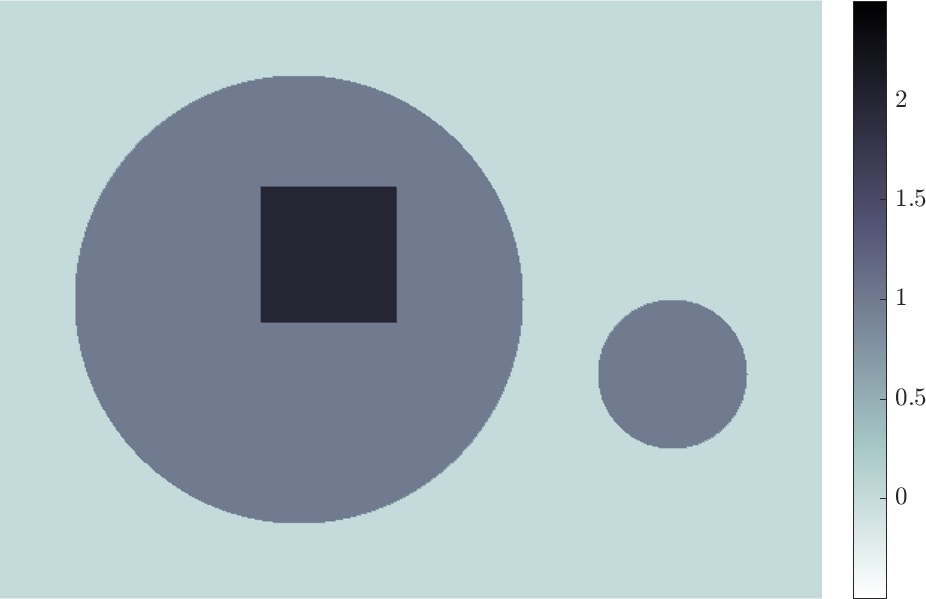
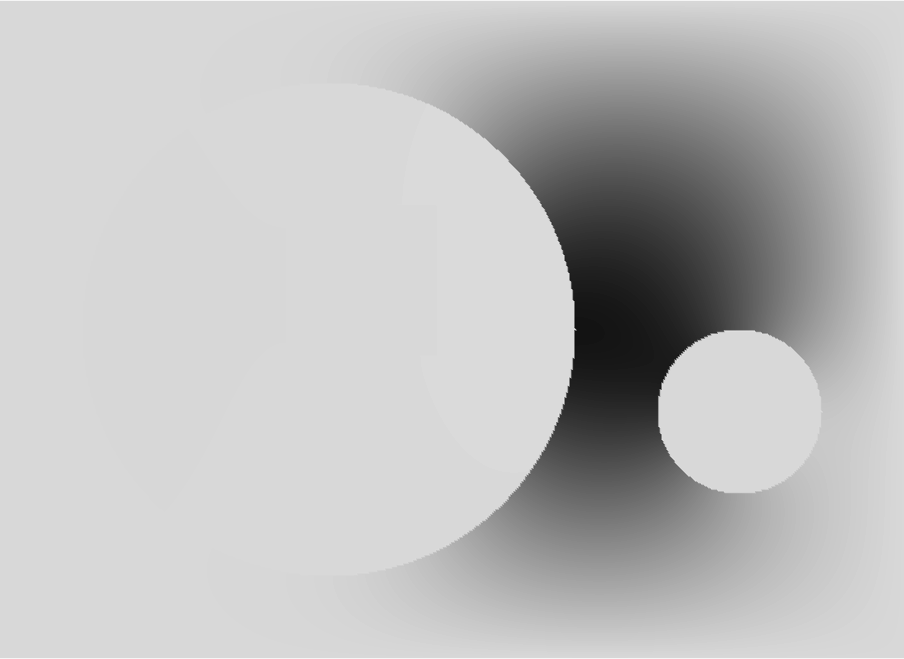
To illustrate the AS decomposition, consider the piecewise constant function shown in Figure 1(a). Next, we (numerically) solve the eigenvalue problem (3.2) with using a -FE discretization with mesh-size . As shown in Figure 2, the first three eigenfunctions , capture the inclusions rather well, whereas the subsequent eigenfunctions resemble eigenfunctions of the Laplacian with eigenvalues that scale as . Next, we project into . As shown in Figure 1(b), the projection is hardly distinguishable from .
In [1, 2], rigorous -error bounds were derived for the AS decomposition. More precisely, consider a piecewise constant function with zero boundary values of the form
| (3.5) |
where is the characteristic function of Lipschitz domains with mutually disjoint and connected boundaries .
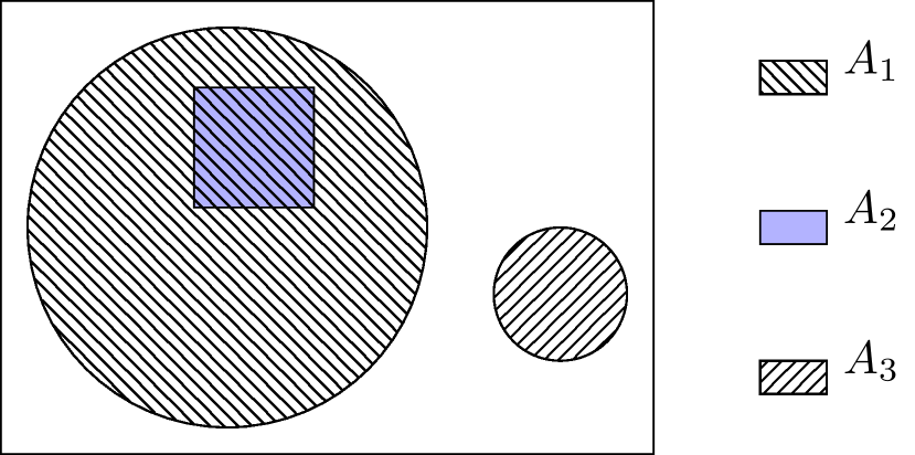
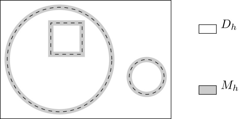
Next we partition into the two open sets
| (3.6) |
where is the open tube with diameter around the jump discontinuities of . In Figure 3, for instance, the sets , , and are shown for as in Figure 1(a).
Clearly, the FE-interpolant of satisfies and in . Moreover, for a sequence of regular and quasi-uniform meshes , we have
| (3.7) |
and with independent of , [1, Proposition 2.2]. In [2], those properties led to the following upper bound for the first eigenfunctions.
Theorem 3.1.
Let be given by (3.5), be its FE interpolant, and , the eigenfunctions of the AS operator . Then, for every and sufficiently small, there exists a constant , independent of and , such that
| (3.8) |
From Theorem 3.1 we conclude that the first eigenfunctions of are almost piecewise constant in , that is away from any discontinuities, when is piecewise constant with inclusions. This indicates that the AS decomposition (3.3) is able to approximate well throughout , which was proved in [1]:
Theorem 3.2.
Let be given by (3.5), be its FE interpolant, , the eigenfunctions of the operator and be its projection. Then, for every and sufficiently small, there exists a constant , independent of and , but possibly depending on , such that
| (3.9) |
In summary, the AS decomposition of approximates arbitrarily well, when is piecewise constant and consists of inclusions. Note that more general versions of Theorem 3.1 and Theorem 3.2 were proved in [2, Theorem 5] and [1, Theorem 3.6], which also apply to piecewise constant functions with nonzero boundary values.
Finally, we remark that the operator corresponds to the Fréchet derivative of the regularized TV-functional, , which reduces to the standard TV-functional for – see [17, Remark 1]. In fact, for , , the “energy-norm” associated to the operator essentially corresponds to the TV-“energy”,
| (3.10) |
The AS decomposition also bears a remarkable resemblance to the spectral decomposition of the nonlinear -functional [6, 14].
4 Adaptive Spectral Inversion
We shall now combine the simple Adaptive Inversion iteration from Section 2 with the AS decomposition (3.3) from Section 3. Hence, at each iteration, we shall determine the new search space from the current minimizer using the eigenfunctions of the elliptic operator in (3.2). Here, we recall from Theorems 3.1 and 3.2 in Section 3 that a piecewise constant medium with inclusions is approximated with high accuracy by the first eigenfunctions of – see also [1, 2] for further details.
First, we merge the current search space with those eigenfunctions and reduce its dimension, while ensuring that is still well represented in the merged space. This first step corresponds to the algorithm previously used in [2] – See Remark 2 below for further details.
Next, to incorporate the new angle condition (2.4) required for Theorem 2.1, we shall include in the most sensitive eigenfunctions reordered according to their sensitivities:
| (4.1) |
We shall now construct a subspace , which contains at least one that satisfies the angle condition (2.4), for a fixed .
Lemma 4.1.
Proof.
Since the eigenfunctions are orthonormal, we have which yields
| (4.3) | ||||
| (4.4) | ||||
| (4.5) | ||||
| (4.6) |
Thus, the angle condition (2.4) is satisfied. ∎
Note that for there always exists sufficiently large such that (4.2) is satisfied.
Lemma 4.2.
Proof.
We refer to (4.2) as the -criterion and to (4.7) as the -criterion. If we let
| (4.11) |
we ensure that there exists at least one element in the subspace that satisfies the newly introduced angle condition (2.4). Clearly, (4.2) is more stringent than (4.7) and thus . As we only compute in practice a finite number of eigenfunctions , , ordered according to their eigenvalues, none might in fact satisfy (4.2). Then we set and thereby in (4.11). In the unlikely case that no satisfies (4.7), one needs to increase until (4.7) holds to ensure the existence of which satisfies (2.4). This yields the full Adaptive Spectral Inversion (ASI) Algorithm below.
| (4.12) |
By combining the previous search space with promising new search directions determined from the current iterate , Steps 6 – 8 construct a low-dimensional subspace able to represent up to a small error. In Step 9, we then add the basis functions which will probably contribute most to the reduction of the misfit. Below, we discuss in detail Steps 6 – 9 of the ASI Algorithm 2.
Step 6: Determine .
Once the minimizer of in the current search space of dimension has been found, we compute the first few eigenfunctions of the elliptic operator , that is, we numerically solve the (linear, symmetric and positive definite) eigenvalue problem (3.2), which yields the new AS basis . Here we arbitrarily set the dimension of to that of , though any other sufficiently large number of eigenfunctions could be chosen.
Step 7: Merge.
Next we merge the previous search space with as and compute an -orthonormal basis , , of via modified Gram-Schmidt. Since the dimension of the merged subspace may be as large as , we now need to truncate to keep the number of control variables small.
Step 8: Truncate.
To truncate and retain only those basis functions essential for representing , we proceed in two steps. First, we compute an indicator close to , but with minimal -“energy”, to remove noise and preserve edges. In doing so, we keep the computational costs low by minimizing the linearized -functional (3.10). Thus, the indicator satisfies
| (4.13) | ||||
for a prescribed truncation tolerance ; typically, . Since (4.13) is a quadratic optimization problem with quadratic inequality constraints, computing is cheap.
Second, we reduce the dimension of by discarding all basis functions that do not contribute much to the indicator . Let denote the Fourier coefficients of ,
| (4.14) |
sorted in decreasing order and sort the -orthonormal basis functions accordingly. Next, we determine the index
| (4.15) |
such that the relative -error in the Fourier expansion truncated at is below . To avoid drastic changes in the dimension of the search space, we now calculate . For prescribed such that , typically and , we choose the dimension of the truncated space as follows:
-
(i)
If , set .
-
(ii)
If , the dimension decreases too fast. Set and halve to avoid a rapid decrease in the dimension at the next iteration.
-
(iii)
If , the dimension increases too fast. Set and double to avoid a rapid increase in the dimension at the next iteration.
This yields the truncated space as .
Step 9: Add sensitivities.
Finally, we determine the most sensitive AS basis functions from , reorderd according to their sensitivities as in (4.1). In doing so, we use the - and -criteria (4.2) and (4.7) from Lemmas 4.1 and 4.2, respectively, to determine . In the unlikely event that the AS space from Step 6 contains no eigenfunction that satisfies (4.2) or (4.7), we can either increase the dimension of , or set (and simply proceed). By combining and , we eventually obtain the subsequent search space
| (4.16) |
Note that the sensitivity based selection procedure in Step 9 only ensures that the angle condition (2.4) is satisfied by at least one element in , but not necessarily by the defect itself. The latter, stronger condition would require verifying (2.4) at every iteration, and possibly rejecting the new minimizer of (4.12) when not satisfied, while further increasing the search space. Instead, Lemmas 4.1 and 4.2 guarantee that at least one element in the search space satisfies the angle condition, thereby making it rather likely that it will also be satisfied by the correction .
Remark 2.
In the above Adaptive Spectral Inversion (ASI) Algorithm, Steps 1 – 8 correspond to the ASI Algorithm previously introduced in [2], yet with the added growth control on in Step 8 (iii). Step 9, however, where further eigenfunctions are included based on their sensitivites (4.1), is new and will prove crucial for detecting small-scale features in the medium. Henceforth we denote by the above ASI Algorithm without Step 9, similar to that from [2], to distinguish it from the present ASI Algorithm.
5 Numerical Results
To illustrate the accuracy and usefulness of the ASI Algorithm from Section 4, we shall now apply it to two inverse medium problems of the form: Find that satisfy
| (5.1) | ||||
| s.t. | (5.2) |
for a given source and noisy data as in (1.2). Each inverse problem is governed by a distinct forward problem (5.2) whose solution, for any given medium333We refer to a function as a medium. , is . Thus, we can eliminate the constraint (5.2), which leads to the equivalent unconstrained minimization problem: Find such that
| (5.3) |
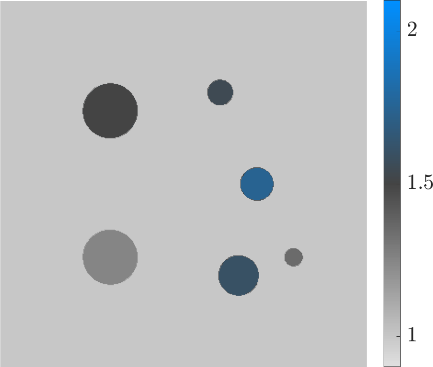
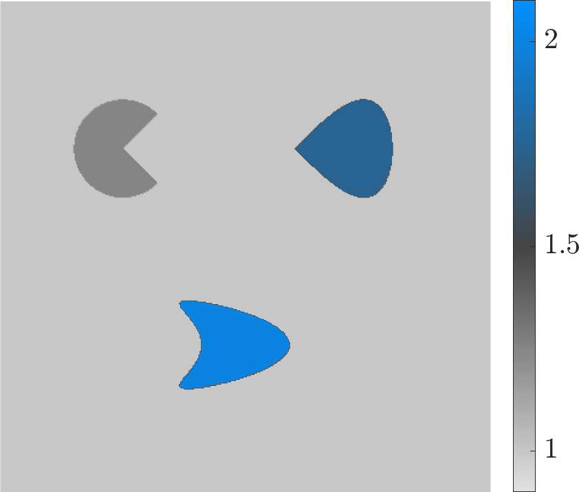
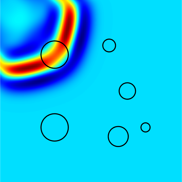
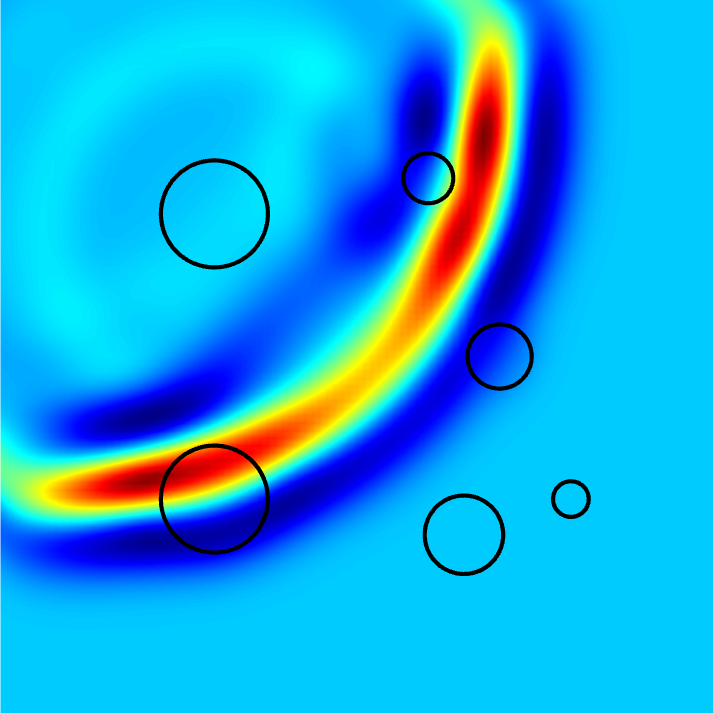
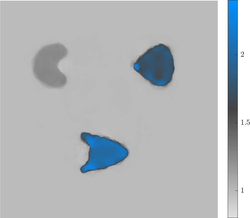
For each inverse problem, we shall attempt to recover separately the two different (unknown) media shown in Figure 4. The first consists of six discs, each with a different value and radius. The second consists of three inclusions: an open wedge with a sharp interior angle, a convex drop-like inclusion with a sharp tip, and a kite-shaped inclusion, which is non-convex with a smooth boundary. Since the unknown medium must be strictly bounded away from zero, we write for with zero boundary. Then, we apply the ASI Algorithm 2 to minimize the misfit
| (5.4) |
with equal to zero at the boundary.
In all cases, we apply the ASI Algorithm 2 from Section 4 with the following fixed parameter settings:
| (5.5) |
As initial guess, we always choose constant and set the initial search space equal to the first or -orthonormal eigenfunctions of the Laplacian sorted in non-decreasing order w.r.t. their eigenvalues.
To assess the accuracy of the ASI method, we shall monitor the following quantities: The dimension of the search space , the relative error
| (5.6) |
the ratio from (2.20),
| (5.7) |
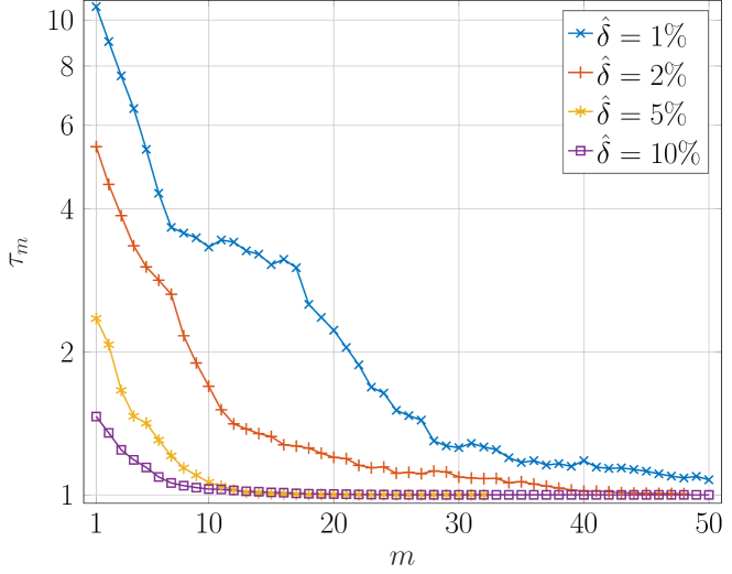
and the total number of iterations , where is the first index such that ; hence, the discrepancy principle (2.20) is then satisfied with .
5.1 Elliptic Inverse Problem
First, we consider as forward problem the elliptic differential equation
| (5.8) |
in the unit square with constant right-hand side ; hence, the observations are available throughout . In [24, 25, 35], the one-dimensional version of (5.8) was considered and shown to satisfy the Scherzer condition (2.27).
Here we shall compare the ASI Algorithm 2 from Section 4 with a standard grid-based inversion method using Tikhonov regularization. We initialize the ASI method with the constant initial guess and let equal the first Laplace eigenfunctions. The forward problem (5.8) is solved in , where corresponds to the subspace of continuous, piecewise linear finite elements (FE) with mesh size . Here, we use for both and the same fixed triangular mesh with vertices located on a equidistant Cartesian grid. Despite the large number () of dof’s in the FE representation, we recall that the ASI Algorithm determines the -th iterate only in the much smaller subspace of dimension . In the -th step of the ASI Algorithm the minimizer to (4.12) is determined using standard BFGS together with Armijo [36] instead of Wolfe-Powell line search to keep the number of (expensive) gradient evaluation small.
For the standard Tikhonov -regularization approach, we minimize
| (5.9) |
where denotes the regularization parameter. Again, we discretize and with -FE on the same triangular mesh as for the ASI method, yet due to the resulting large number of unknowns, we now solve (5.9) using standard limited memory BFGS (L-BFGS) [36] together with Armijo line search. Following [12, Section ], we set the regularization parameter at the -th L-BFGS iteration.
To avoid any potential inverse crime, the exact data was computed from a finer mesh and perturbed at each grid point as
| (5.10) |
for a noise level . Here, corresponds to Gaussian noise normalized such that the data misfit with satisfies exactly
| (5.11) |
| Method | ASI | -regularization | ||||||
|---|---|---|---|---|---|---|---|---|
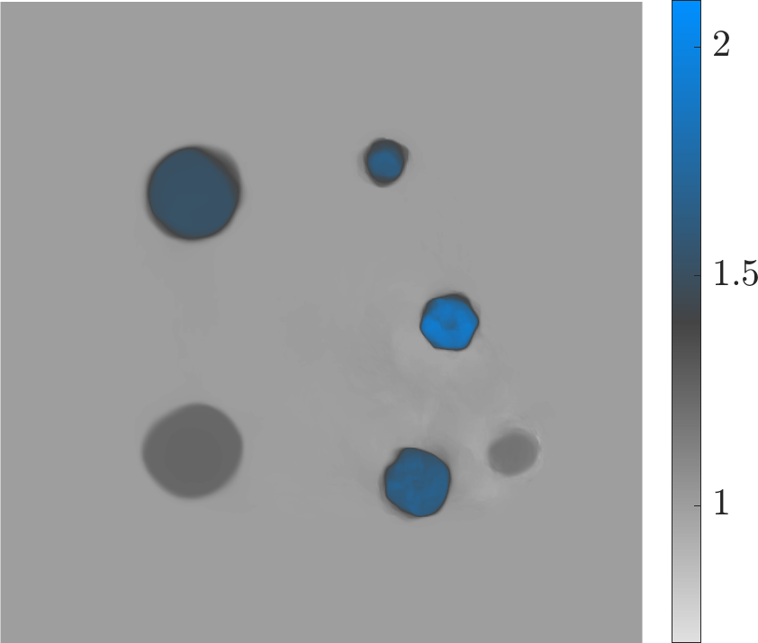
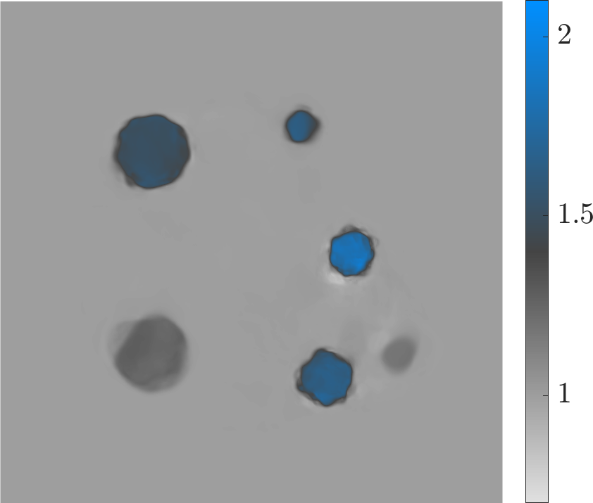
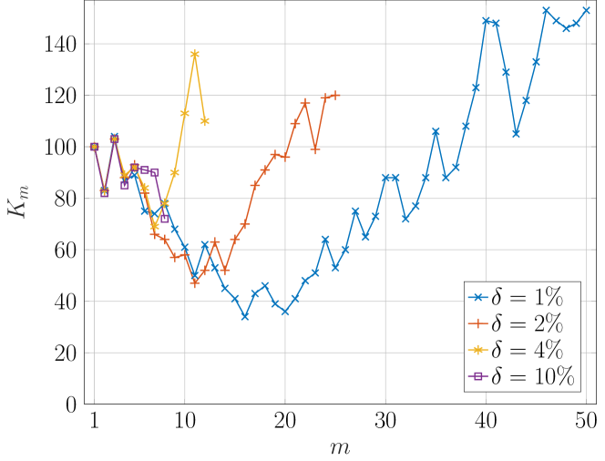
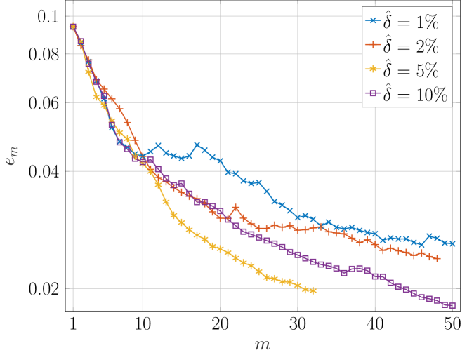
In Table 1 we list the relative error at the final iteration for the ASI method and -Tikhonov regularization together with the dimension of the search space . As expected, both methods require fewer iterations to achieve (2.20) as the noise level increases, while the relative error obtained by the ASI method is always smaller than that achieved by standard -Tikhonov regularization. Even with the ASI method yields a smaller relative error than standard Tikhonov regularization using smaller . In Figure 5, we compare the reconstructed media for the two methods. Clearly, the reconstruction obtained by the ASI method displays sharper contrasts and crisper edges while the coefficients inside each disc are more accurate. Moreover, for -Tikhonov regularization, the background appears noisy and the coefficients inside the inclusions are not accurately reconstructed. Remarkably, the better reconstruction obtained by the ASI method is achieved with as few as control variables only, in contrast to grid-based Tikhonov regularization with more than unknowns.
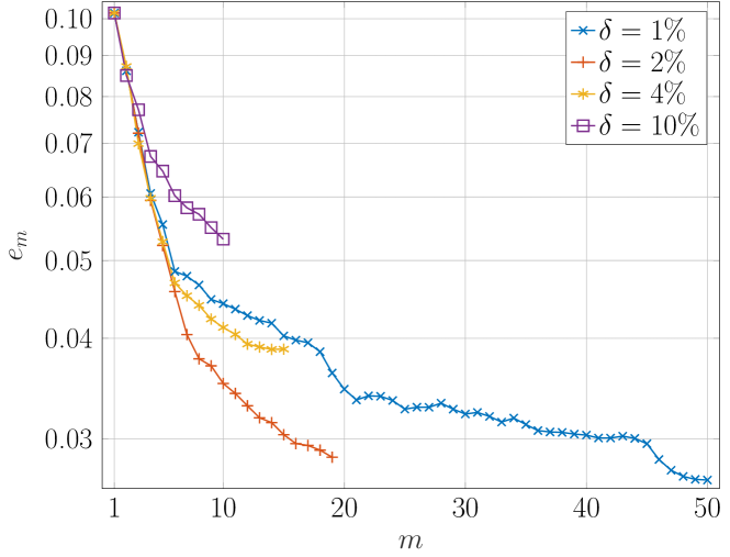
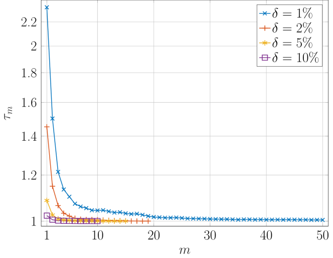
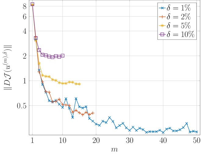
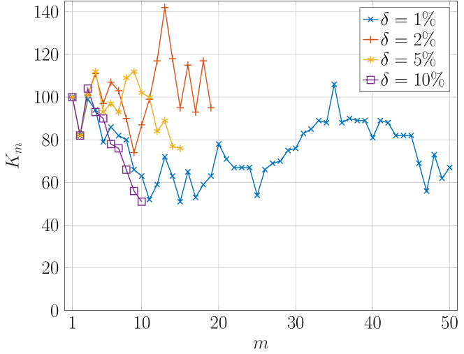
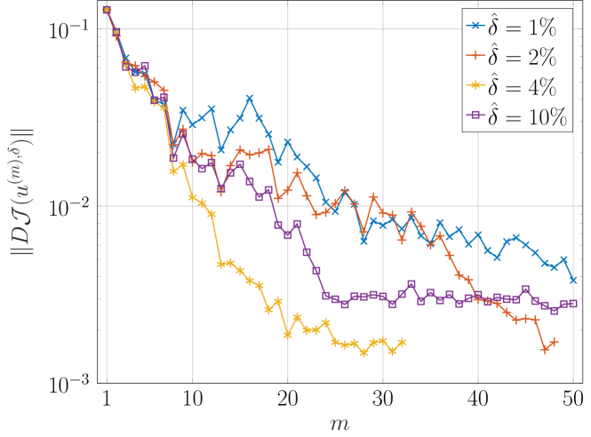
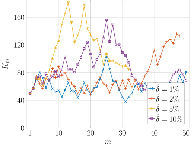
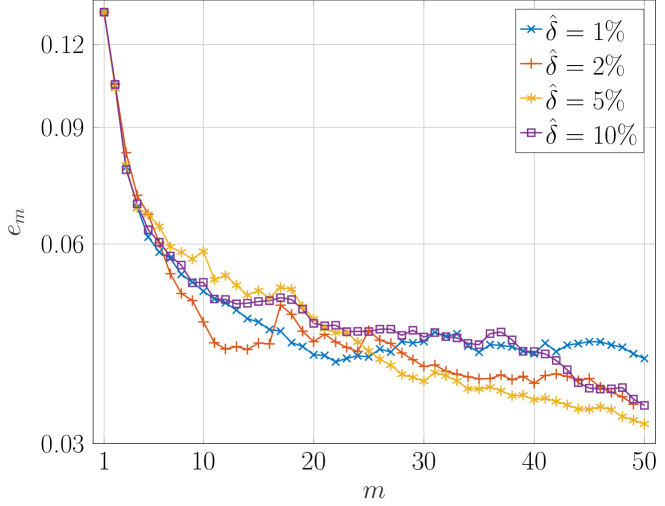
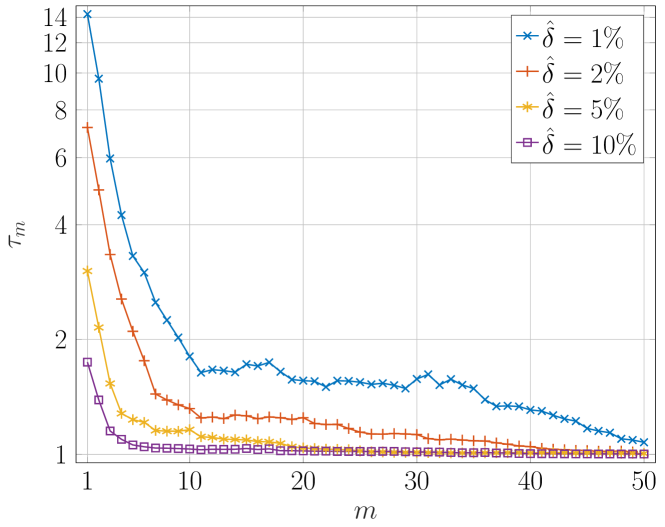
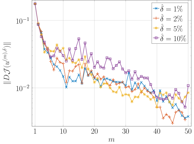
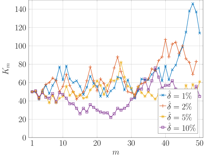
In Figure 6, we observe that the relative error and decrease throughout all iterations, as expected from Theorem 2.1 in Section 2, while tends to . Note that the dimension , or equivalently the number of control variables, remains small for the ASI method regardless of , which keeps the computational effort low.
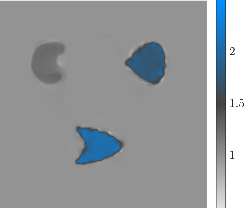
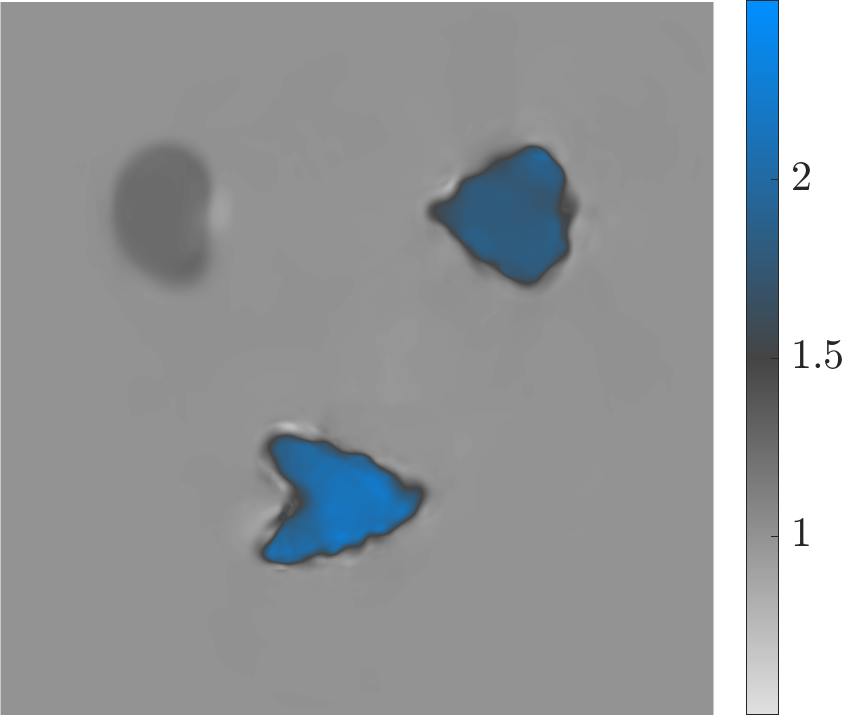
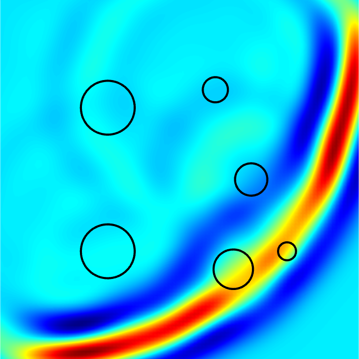
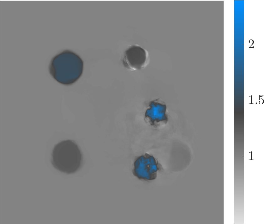
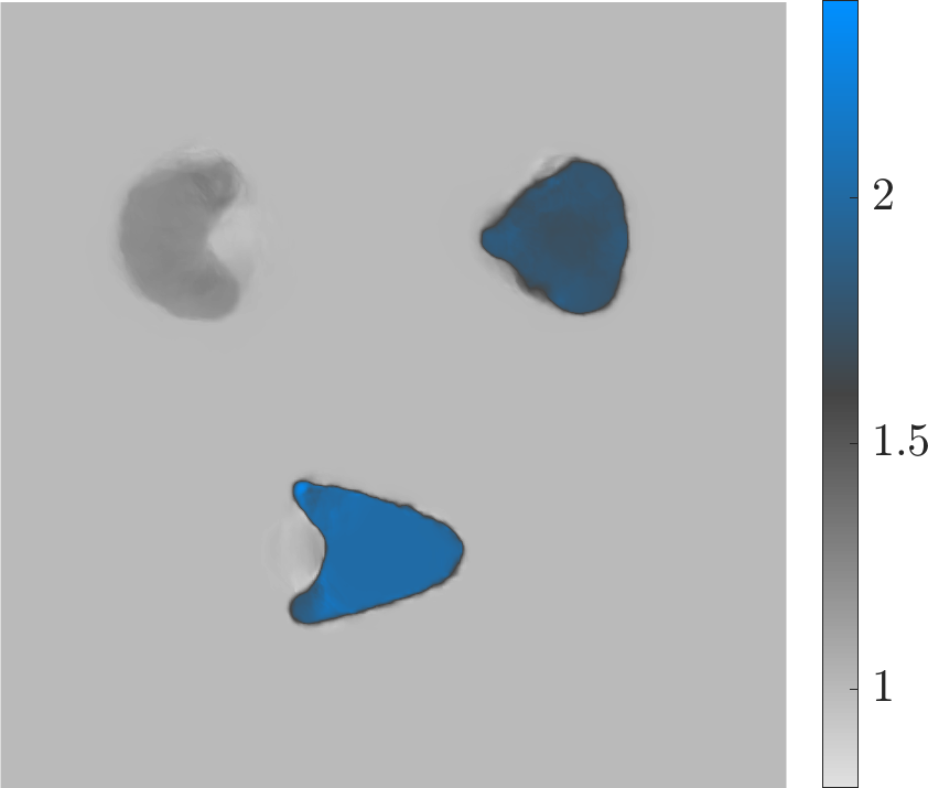
Next, we consider the (unknown) medium shown in the right frame of Figure 4, which consists of three distinct inclusions. Again, the ASI Algorithm from Section 4 is able to recover the medium at the various noise levels , as shown in Figure 7: all three inclusions are clearly visible with good contrast and sharp edges, except for the reentrant corner of the open wedge with noise. -Tikhonov regularization, however, results in more noisy and blurred reconstructions, where the inclusions become hardly visible beyond noise.
From Table 2, we again infer that the relative error of the ASI method alway remains below that obtained with -Tikhonov regularization: Even with noise, the ASI method remains more accurate than -Tikhonov regularization with as little as noise. Moreover, the number of control variables used in the ASI method never exceeds , in comparison to approximately control variables used in the nodal FE representation for -Tikhonov regularization. As a consequence, the computational effort of the ASI method always remains well below that with standard Tikhonov regularization.
In Figure 8, we observe that the relative error and decrease with each iteration, while the ratio tends to and the number of basis functions of the search space , i.e. the number of control variables, remains small, which again translates to a low computational effort. Note that implies that (nearly) yields an optimal data misfit because .
| Method | ASI | -regularization | ||||||
|---|---|---|---|---|---|---|---|---|

5.2 Time Dependent Inverse Scattering Problem
Next, we consider wave scattering from an unknown spatially distributed medium illuminated by surrounding point sources. Hence, the forward problem (5.2) now corresponds to the time-dependent wave equation in ,
| (5.12) |
with homogeneous initial conditions and first-order absorbing boundary conditions. Here, denotes the squared wave speed whereas the sources , , correspond to smoothed Gaussian point sources
| (5.13) |
in space, centered about distinct locations , with and , and a Ricker wavelet [10, 30] in time,
| (5.14) |
with central frequency . In Figure 9, snapshots of the solution to the forward problem (5.12) are shown at different times for the source located at the top left corner.
The forward problem (5.12) is solved by a standard Galerkin-FE method, where we again discretize using piecewise linear -FE on a triangular mesh with vertices located on a equidistant Cartesian grid. For in (5.12), however, we use quadratic -FE with mass-lumping [7, 32] on a separate triangular mesh with about elements per wavelength, resulting in approximately nodes. For the time integration, we use the standard (fully explicit) leapfrog method with time-step .
To generate the (synthetic) observations, we now place sources located at equidistributed near the boundary and illuminate the medium, one source at a time. In contrast to the previous example from Section 5.1, here the data is only available at the boundary nodes, yet for all discrete time-steps , , until the final time when the incident wave has essentially left . Hence, we set and in (5.3), where the misfit
| (5.15) |
now accounts for the data from multiple sources .
To avoid any potential inverse crime, the exact data was computed from a finer mesh. The perturbed (noisy) data was then obtained at each boundary node and time-step as
| (5.16) |
for a noise level . Here, corresponds to normally distributed Gaussian noise with
| (5.17) |
To reduce computational cost during the inverse iteration, we do not minimize (5.15) directly, but instead use a standard sample average approximation (SAA) [19]: at each iteration, we combine all sources into a single “super-shot” ,
| (5.18) |
where follow a Rademacher distribution with zero mean. Thus, at each iteration , we solve the minimization problem
| (5.19) |
with corresponding boundary observations
| (5.20) |
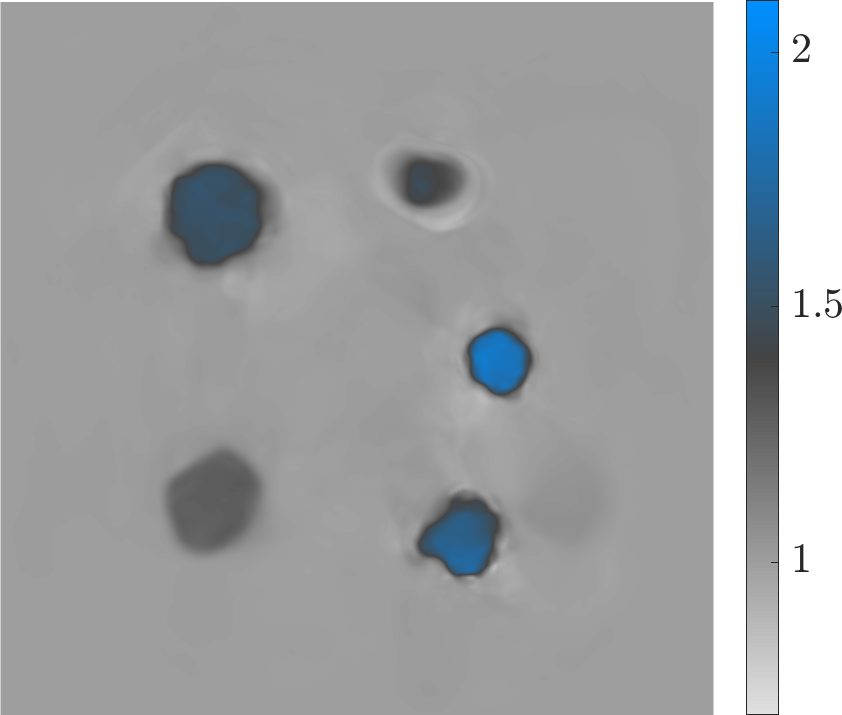
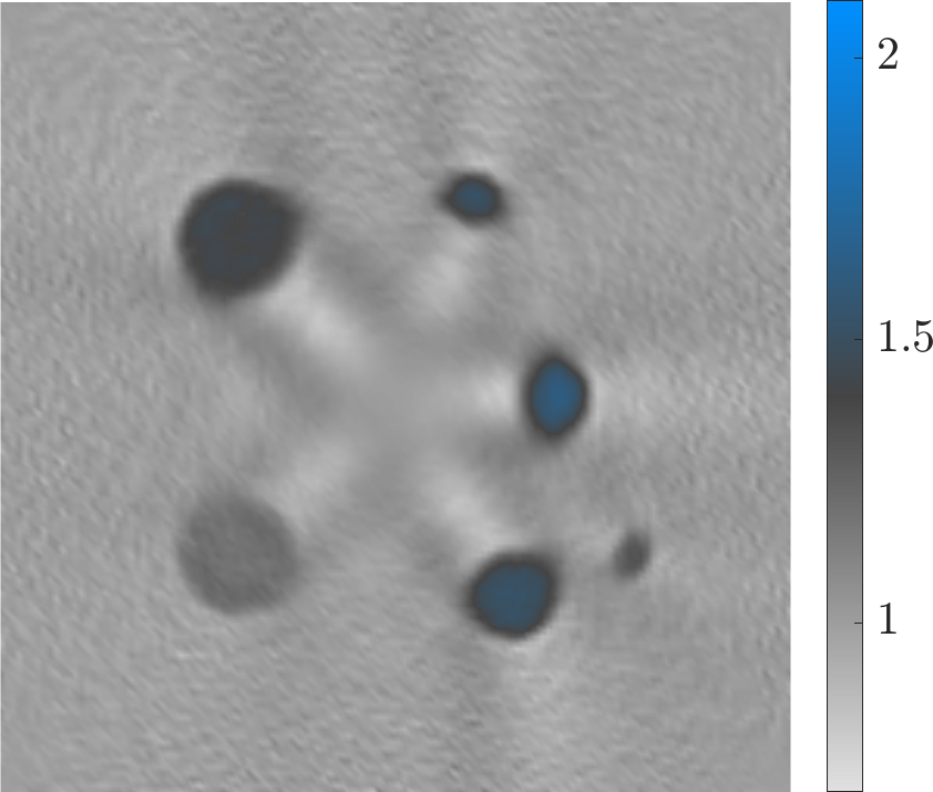
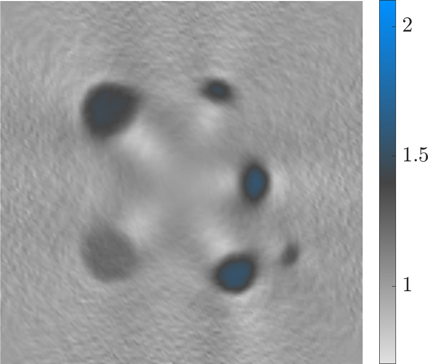
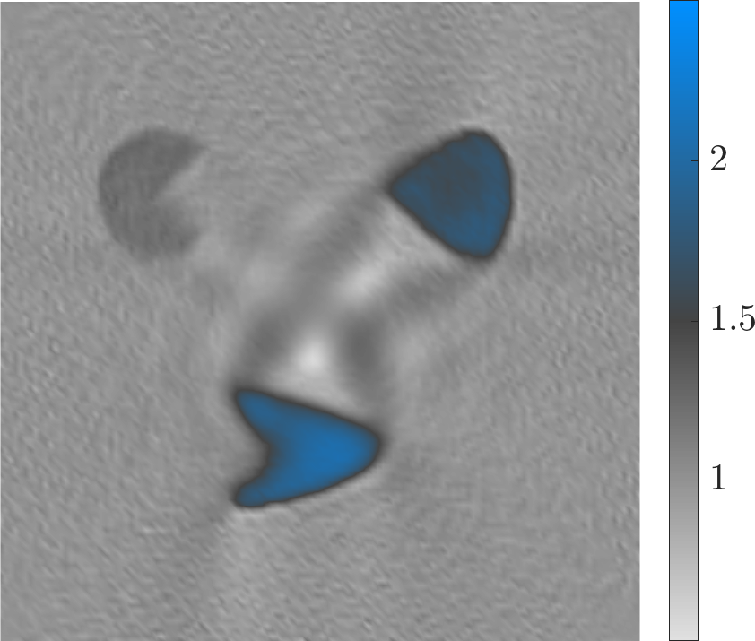
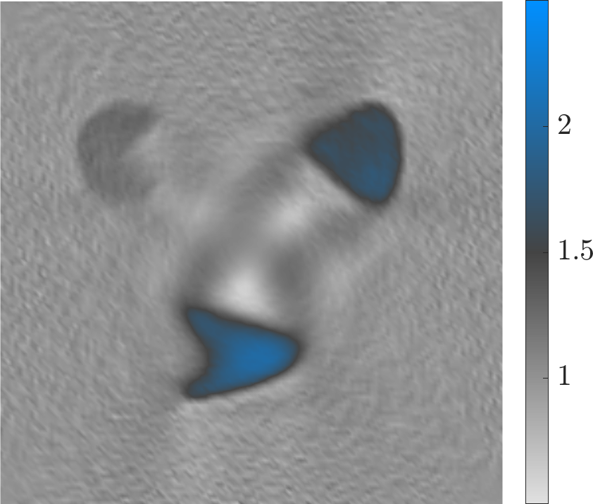
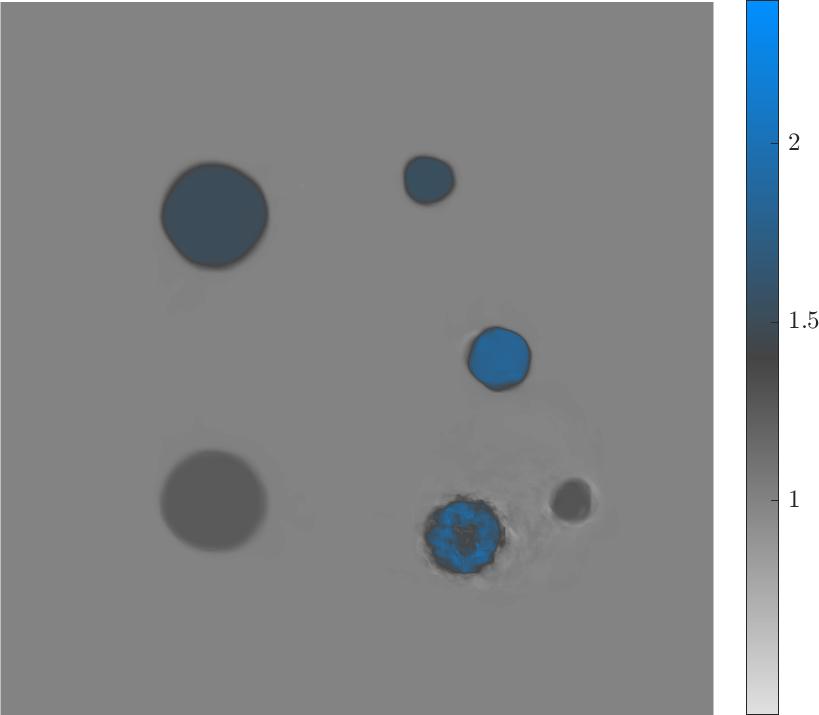
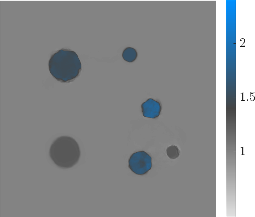
First, we compare the ASI Algorithm from Section 4 with the former Algorithm, where we omit Step 9 and thus ignore the most sensitive AS basis functions required for the angle condition, see Remark 2. To do so, we consider the (unknown) medium consisting of six discs shown in Figure 4. In Table 3, we observe that the ASI and Algorithms perform similarly in terms of the relative error and dimension of the search space . However, when we compare the reconstructed media from Figure 10, we observe that the Algorithm (bottom row) fails to reconstruct the smallest disc with increasing noise, whereas the ASI Algorithm (top row) always recovers even that smallest disc.
In Figure 11, the relative error decreases throughout all iterations, while , and hence the number of control variables, remains small, which keeps the overall computational cost low. As expected from Theorem 2.1, the norm of the gradient decreases and the ratio from the discrepancy principle (5.7) tends to 1.
| Method | ASI | |||||||
|---|---|---|---|---|---|---|---|---|


Finally, we consider the medium shown in Figure 4 with three geometric inclusions. As shown in Figure 12, the ASI Algorithm recovers the shape and height of all three inclusions with high fidelity and regardless of the noise level . In Table 4 and Figure 13, we observe that the relative error remains low for all and decreases throughout all iterations. Again, the ratio from (5.7) tends to while decreases. For all noise levels , the number of basis functions never exceeds , which greatly reduces the computational effort compared to a standard nodal based optimization approach with control variables. Since the ASI and Algorithms performed similarly, the results from the latter are omitted here.
| Method | ASI | |||
|---|---|---|---|---|

6 Concluding Remarks
The Adaptive Spectral Inversion (ASI) method has proved remarkably effective for the solution of PDE-constrained inverse medium problems. At the -th iteration, the ASI method minimizes the data misfit with added noise in a small subspace , which inherits key information from the previous step while adding promising new search directions from the first few eigenfunctions of the elliptic operator in (3.2). Since the operator itself depends on the current iterate, , so do its eigenfunctions and thus also the new search space . The convergence of the ASI method hinges upon the angle condition (2.4) – see Theorem 2.1 – which has been newly included as a final step into each iteration. The full ASI Algorithm 2 is listed in Section 4.
Under suitable assumptions, the ASI iteration stops after (finitely many) iterations when the discrepancy principle (2.20) is satisfied. Hence, the ASI Algorithm yields a genuine regularization method whose solution converges to the exact (noise-free) solution as , without the need for extra Tikhonov regularization – see Theorem 2.3. By adapting the search space at each iteration while keeping its dimension low, the ASI method achieves more accurate reconstructions than standard grid-based Tikhonov -regularization together with a thousandfold decrease in the number of unknowns. Thanks to the newly incorporated angle condition (2.4), the ASI Algorithm is able to detect even the smallest inclusions in the medium, which previous versions of the algorithm [18] at times failed to identify with increasing noise.
The added cost from the numerical solution of the eigenvalue problem (3.2) is rather small. On the one hand, the Galerkin FE discretization leads to a generalized eigenvalue problem which is sparse, symmetric, and positive definite. On the other hand, we only require a few eigenfunctions which can be efficiently computed by a standard Lanczos iteration. A further reduction in the computational cost can easily be achieved by using an adaptively refined FE mesh when solving (3.2), as in [17], which need not coincide with the mesh used for discretizing the governing PDE. As the higher eigenfunctions become increasingly localized, they can easily be “sparsified” simply by setting to zero the smallest coefficients in their discrete FE representation [17].
Although we have concentrated here on two-dimensional inverse medium problems, the AS decomposition in fact applies to arbitrary many space dimensions [1]. When the target medium is not piecewise constant but instead smoothly varying, adaptive spectral bases resulting from different elliptic operators may be more effective [18]. Clearly, the ASI approach would probably prove useful for inverse source problems, for instance, or could be be combined with alternative (globally convergent) inversion methods [5]. It could also be applied to other inverse problems, unrelated to wave scattering, where the state variable is governed by a different partial differential, or possibly even integral, equation.
Acknowledgments.
We thank Daniel Baffet for useful comments and suggestions.
References
- [1] D. H. Baffet, Y. G. Gleichmann, and M. J. Grote, Error estimates for aptive spectral decompositions, Journal of Scientific Computing, 93 (2022).
- [2] D. H. Baffet, M. J. Grote, and J. H. Tang, Adaptive spectral decompositions for inverse medium problems, Inverse Problems, 37 (2021), p. 025006.
- [3] A. B. Bakushinsky and M. Y. Kokurin, Iterative Methods for Approximate Solution of Inverse Problems, Springer Netherlands, 2004.
- [4] H. H. Bauschke and P. L. Combettes, Convex Analysis and Monotone Operator Theory in Hilbert Spaces, Springer International Publishing, 2017.
- [5] L. Beilina and M. V. Klibanov, Approximate Global Convergence and Adaptivity for Coefficient Inverse Problems, Springer US, 2012.
- [6] M. Burger, G. Gilboa, M. Moeller, L. Eckardt, and D. Cremers, Spectral decompositions using one-homogeneous functionals, SIAM Journal on Imaging Sciences, 9 (2016), pp. 1374–1408.
- [7] G. Cohen, P. Joly, J. E. Roberts, and N. Tordjman, Higher order triangular finite elements with mass lumping for the wave equation, SIAM Journal on Numerical Analysis, 38 (2001), pp. 2047–2078.
- [8] I. Daubechies, M. Defrise, and C. De Mol, An iterative thresholding algorithm for linear inverse problems with a sparsity constraint, Communications on Pure and Applied Mathematics, 57 (2004), pp. 1413–1457.
- [9] M. de Buhan and M. Darbas, Numerical resolution of an electromagnetic inverse medium problem at fixed frequency, Computers & Mathematics with Applications, 74 (2017), pp. 3111–3128.
- [10] M. de Buhan and M. Kray, A new approach to solve the inverse scattering problem for waves: combining the TRAC and the adaptive inversion methods, Inverse Problems, 29 (2013), p. 085009.
- [11] M. de Buhan and A. Osses, Logarithmic stability in determination of a 3d viscoelastic coefficient and a numerical example, Inverse Problems, 26 (2010), p. 095006.
- [12] H. W. Engl, M. Hanke, and A. Neubauer, Regularization of Inverse Problems, vol. 375, Springer Science & Business Media, 1996.
- [13] F. Faucher, O. Scherzer, and H. Barucq, Eigenvector models for solving the seismic inverse problem for the Helmholtz equation, Geophysical Journal International, (2020).
- [14] G. Gilboa, M. Moeller, and M. Burger, Nonlinear spectral analysis via one-homogeneous functionals: Overview and future prospects, Journal of Mathematical Imaging and Vision, 56 (2016), pp. 300–319.
- [15] M. Graff, M. J. Grote, F. Nataf, and F. Assous, How to solve inverse scattering problems without knowing the source term: a three-step strategy, Inverse Problems, 35 (2019), p. 104001.
- [16] C. W. Groetsch and A. Neubauer, Convergence of a general projection method for an operator equation of the first kind, Houston J. Math., 14 (1988), pp. 201–208.
- [17] M. J. Grote, M. Kray, and U. Nahum, Adaptive eigenspace method for inverse scattering problems in the frequency domain, Inverse Problems, 33 (2017), p. 025006.
- [18] M. J. Grote and U. Nahum, Adaptive eigenspace for multi-parameter inverse scattering problems, Computers & Mathematics with Applications, 77 (2019), pp. 3264–3280.
- [19] E. Haber, M. Chung, and F. Herrmann, An effective method for parameter estimation with PDE constraints with multiple right-hand sides, SIAM Journal on Optimization, 22 (2012), pp. 739–757.
- [20] U. Hämarik, E. Avi, and A. Ganina, On the solution of ill-posed problems by projection methods with a posteriori choice of the discretization level, Math. Model. Anal., 7 (2002), pp. 241–252.
- [21] M. Hanke, A. Neubauer, and O. Scherzer, A convergence analysis of the Landweber iteration for nonlinear ill-posed problems, Numerische Mathematik, 72 (1995), pp. 21–37.
- [22] F. J. Herrmann and G. Hennenfent, Non-parametric seismic data recovery with curvelet frames, Geophys. J. Int., (2008), pp. 233–248.
- [23] B. Hofmann, P. Mathé, and S. V. Pereverzev, Regularization by projection: Approximation theoretic aspects and distance functions, Journal of Inverse and Ill-posed Problems, 15 (2007).
- [24] B. Kaltenbacher, Regularization by projection with a posteriori discretization level choice for linear and nonlinear ill-posed problems, Inverse Problems, 16 (2000), pp. 1523–1539.
- [25] B. Kaltenbacher, A. Neubauer, and O. Scherzer, Iterative Regularization Methods for Nonlinear Ill-Posed Problems, De Gruyter, 2008.
- [26] B. Kaltenbacher and J. Offtermatt, A convergence analysis of regularization by discretization in preimage space, Math. Comput., 81 (2012), pp. 2049–2069.
- [27] A. Kirsch, An Introduction to the Mathematical Theory of Inverse Problems, vol. 120 of Applied Mathematical Sciences, Springer-Verlag, New York, 1996.
- [28] L. Landweber, An iteration formula for Fredholm integral equations of the first kind, American Journal of Mathematics, 73 (1951), pp. 615–624.
- [29] Y. Lin, A. Abubakar, and T. M. Habashy, Seismic full-waveform inversion using truncated wavelet representations, (2012), pp. 1–6. SEG Annual meeting 2012, Las Vegas.
- [30] C. D. Lines and S. N. Chandler-Wilde, A time domain point source method for inverse scattering by rough surfaces, Computing, 75 (2005), pp. 157–180.
- [31] I. Loris, H. Douma, G. Nolet, I. Daubechies, and C. Regone, Nonlinear regularization techniques for seismic tomography, Journal of Computational Physics, (2010), pp. 890–905.
- [32] W. A. Mulder, Higher-order mass-lumped finite elements for the wave equation, Journal of Computational Acoustics, 09 (2001), pp. 671–680.
- [33] F. Natterer, Regularisierung schlecht gestellter Probleme durch Projektionsverfahren, Numerische Mathematik, 28 (1977), pp. 329–341.
- [34] C. Sanders, M. Bonnet, and W. Aquino, An adaptive eigenfunction basis strategy to reduce design dimension in topology optimization, Internat. J. Numer. Methods Engrg., 122 (2021), pp. 7452–7481.
- [35] O. Scherzer, H. W. Engl, and K. Kunisch, Optimal a posteriori parameter choice for Tikhonov regularization for solving nonlinear ill-posed problems, SIAM Journal on Numerical Analysis, 30 (1993), pp. 1796–1838.
- [36] S. Wright and J. Nocedal, Numerical Optimization, Springer New York, 2006.