Emergent rate-based dynamics in duplicate-free populations of spiking neurons

Abstract

Can the dynamics of Spiking Neural Networks (SNNs) approximate the dynamics of Recurrent Neural Networks (RNNs)? Arguments in classical mean-field theory based on laws of large numbers provide a positive answer when each neuron in the network has many “duplicates”, i.e. other neurons with almost perfectly correlated inputs. Using a disordered network model that guarantees the absence of duplicates, we show that duplicate-free SNNs can converge to RNNs, thanks to the concentration of measure phenomenon. This result broadens the mechanistic plausibility of rate-based theories in neuroscience.

Neurons in the brain interact via spikes – short and stereotyped membrane potential deflections – commonly modeled as Dirac pulses [RieWar97, GerKis02]. SNNs with recurrent connectivity are simplified models of real networks with the essential biological feature of spike-based neuronal communication. On the contrary, traditional RNNs are continuous dynamical systems where abstract rate neurons directly transmit their firing rate to other neurons, a type of communication which is not biological. Despite their inferior realism, RNNs continue to play a central role in theoretical neuroscience because they can be trained by modern machine learning methods [Bar17], they can be analysed using tools from statistical physics [AmiGut85b, SomCri88, MasOst18, PerAlj23], and because biological networks are believed to implement certain computations by approximation of continuous dynamical systems [VyaGol20]. Closing the gap between the more biological SNNs and the more tractable RNNs requires identifying the conditions under which the continuous dynamics of RNNs can be approximated by SNNs [Bre15].

To clearly state the problem, let us consider an SNN composed of $N$ Poisson neurons (linear-nonlinear-Poisson neurons [Chi01] or nonlinear Hawkes processes [BreMas96]). For each neuron index $i$, the spike times $\{t^{k}_{i}\}_{k}$ of neuron $i$, which define the neuron’s spike train $S_{i}(t)=\sum_{k}\delta(t-t^{k}_{i})$, are generated by an inhomogeneous Poisson process with instantaneous firing rate $\phi(h_{i}(t))$, where $h_{i}(t)$ represents the neuron’s potential and $\phi$ is a positive-valued nonlinear transfer function. The potential $h_{i}(t)$ is a leaky integrator of the recurrent inputs coming from neurons $j\neq i$ and the external input $I^{\mathrm{ext}}_{i}(t)$:

$$\tau\frac{\mathrm{d}}{\mathrm{d}t}h_{i}(t)=-h_{i}(t)+\sum_{j=1}^{N}J_{ij}S_{j}(t)+I^{\mathrm{ext}}_{i}(t),$$ (1)

where $\tau$ is the integration (or membrane) time constant and $J_{ij}$ is the synaptic weight from neuron $j$ to neuron $i$ (by convention, $J_{ii}=0$). While the spike-based model described here is biologically simplistic, it is mathematically convenient as it has a straightforward rate-based counterpart. If we replace the spike trains $\{S_{j}(t)\}_{j}$ in (1) by the corresponding instantaneous firing rates $\{\phi(h_{j}(t))\}_{j}$ (i.e. neurons communicate their firing rate directly), we get the rate-based dynamics

$$\tau\frac{\mathrm{d}}{\mathrm{d}t}x_{i}(t)=-x_{i}(t)+\sum_{j=1}^{N}J_{ij}\phi(x_{j}(t))+I^{\mathrm{ext}}_{i}(t),$$ (2)

which defines an RNN with $N$ rate units. To avoid confusion, we write $h_{i}(t)$ for the potentials of the SNN (1) and $x_{i}(t)$ for the potentials of the RNN (2). While the mapping from the SNN to the RNN looks simple at first glance, the spike-based stochastic process (1) and the rate-based dynamical system (2) describe very different kinds of systems and the SNN potentials $h_{i}(t)$ are not guaranteed, in general, to be equal or even close to the RNN potentials $x_{i}(t)$ even if both networks receive the same external input. Note that if the neurons are uncoupled (i.e. $J_{ij}=0$ for all $i,j$), the SNN potentials $h_{i}(t)$ are trivially equal to the RNN potentials $x_{i}(t)$. Therefore, comparing the SNN and the RNN is meaningful only if the coupling does not vanish. For nontrivial coupling, there are two known types of scaling limits where the SNN potentials $h_{i}(t)$ converge to the RNN potentials $x_{i}(t)$:

1. Spatial averaging over neuronal duplicates: Consider networks of increasing size $N$ where neurons are localized in some fixed space such that two neurons assigned to the same point are duplicates, i.e. they always share the same recurrent and external input. If the synaptic weights are scaled by $1/N$, we can take the mean-field limit $N\to\infty$ [Ger95]. The fixed space can be either discrete and finite [DitLoe17] or continuous and finite-dimensional [CheDua19], e.g. a ring [BenBar95]. These classical mean-field limits rely on a strong form of redundancy: the existence of large ensembles of neuronal duplicates receiving (almost) the same recurrent and external input.

2. Temporal averaging over single-neuron spikes: In (1), we can replace the transfer function $\phi$ and the weights $\{J_{ij}\}_{i\neq j}$ by $b\,\phi$ and $\{J_{ij}/b\}_{i\neq j}$, respectively (for $b>0$), and take the limit $b\to\infty$ [Kur71]. This limit entails arbitrarily high firing rates in the SNN, which is biologically unrealistic since two spikes have to be separated by at least $1$ to $2$ milliseconds (the absolute refractory period) [RieWar97, KanSCh00]. Alternatively, but to a similar effect, we can take the limit $\tau\to\infty$ in both (1) and (2) while re-scaling the weights $\{J_{ij}\}_{i\neq j}$ and the external inputs $I^{\mathrm{ext}}_{i}(t)$ by $1/\tau$. This last limit entails arbitrarily slow network dynamics, which is incompatible with human visual processing speed (less than $150$ milliseconds) [ThoFiz96].

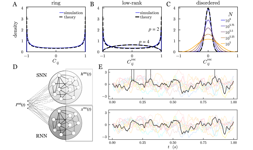
Figure 1: (A) Limit correlation density for the ring model. The histogram of a simulation with $N=10^{6}$ units (solid blue line) is compared to the theoretical limit density (5) (dashed black line). (B) Limit correlation density (of units receiving recurrent input only) for low-rank networks $p=2$ and $p=4$. Simulations of RNNs with $N=10^{6}$ units (solid blue line) are compared to the corresponding theoretical limit “Gegenbauer” density (11) (dashed black line). (C) Concentration around $0$ of the correlation distribution in disordered networks with $p=\alpha N$ and fixed load $\alpha=10^{-4}$. The correlation distribution (of units receiving recurrent input only) of simulations of networks of increasing size $N$ converge to a centred normal density with variance $1/p=1/(\alpha N)$ (the dashed black line indicates the normal density for $N=10^{6}$). (D) Setup for comparing SNNs and RNNs. (E) Trajectories of single-neuron potentials in the SNN ($h^{\mathrm{rec}}_{i}(t)$, upper panel) and in the RNN ($x^{\mathrm{rec}}_{i}(t)$, lower panel) during a one-second simulation of the setup shown in (D). The networks have $N=10^{6}$ neurons and load $\alpha=10^{-4}$, as in (C). The same randomly chosen $11$ neurons are recorded in the SNN and in the RNN and each colour corresponds to a different neuron (the colours in the upper and lower panels correspond). For one neuron (the black trace), the spike times of the neuron in the SNN are indicated by vertical bars. (B-E) Neuronal parameters: $\tau=10$ ms and $\phi(x)=\frac{1}{2\tau}\left(\tanh(x-b)+1\right)$ with $b=2$; input standard deviation is $\sigma=0.5$ (see (9)).

In this letter, we address the following question: can large SNNs, as defined in (1), converge to equally large RNNs in the absence of neuronal duplicates and without temporal averaging?

Temporal averaging as in (ii) is made impossible if we impose, as we do, that

$$\max\phi\leq 1/\tau.$$ (3)

Under this constraint, leaky integration by the potential (1) is too fast to average out the Poisson noise of individual input spike trains and neither of the two scalings mentioned under (ii) can be applied.

To quantify the amount of duplication in an RNN, we look at the distribution of correlations [RenDel10] between pairs of distinct neurons $i\neq j$

$$C_{ij}\mathrel{\mathop{\mathchar 58\relax}}=\lim_{T\to\infty}\frac{1}{T}\int_{0}^{T}\frac{(x_{i}(t)-\overline{x_{i}})(x_{j}(t)-\overline{x_{j}})}{\sigma_{x_{i}}\sigma_{x_{j}}}dt,$$ (4)

where $\overline{x_{i}}$ and $\sigma_{x_{i}}^{2}$ are, respectively, the time average and fluctuation of $x_{i}(t)$ ($\overline{x_{i}}\mathrel{\mathop{\mathchar 58\relax}}=\lim_{T\to\infty}\frac{1}{T}\int_{0}^{T}x_{i}(t)dt$ and $\sigma_{x_{i}}^{2}\mathrel{\mathop{\mathchar 58\relax}}=\lim_{T\to\infty}\frac{1}{T}\int_{0}^{T}(x_{i}(t)-\overline{x_{i}})^{2}dt$.

Based on the correlation distribution, we say that duplicates accumulate in large networks if, as $N\to\infty$, the limit pairwise correlation density has a strictly positive mass around $1$. To illustrate how duplicates accumulate in classical mean-field models, let us consider a toy example with a ring structure. Let the $N$ units of an RNN be uniformly and independently positioned on a ring, $\theta_{i}$ denoting the angular position of unit $i$. If the correlation between unit $i$ and $j$ is given by $C_{ij}\mathrel{\mathop{\mathchar 58\relax}}=\cos(\theta_{i}-\theta_{j})$, then, as $N\to\infty$, the limit distribution of the pairwise correlation, which we call the limit correlation density, is

$$\rho(z)=\mathbbm{1}_{[-1,1]}(z)\frac{1}{\pi}\frac{1}{\sqrt{1-z^{2}}}$$ (5)

(Fig 1A; proof in ). This limit density has a strictly positive mass around $1$, reflecting the fact that each unit has a number of duplicates that grows linearly with $N$.

Conversely, we say that large networks of a given model are duplicate-free if, for any threshold $\varepsilon>0$, the probability that there exists a pair of distinct neurons $i\neq j$ such that their absolute correlation is greater or equal to $\varepsilon$ tends to $0$ as $N\to\infty$, i.e.

$$\forall\varepsilon>0,\quad\mathbb{P}(\exists\,i\neq j\text{ such that }|C_{ij}|\geq\varepsilon)\xrightarrow[N\to\infty]{}0.$$ (6)

In the following, we propose a disordered network model where large networks are duplicate-free.

Input-driven disordered network model.— We construct the connectivity matrix $\mathbf{J}=\{J_{ij}\}_{i,j}$ as a sum of random rank-one matrices (minus self-interaction terms), a construction similar to that of Hopfield networks [Hop82, AmiGut85a, PerBru18]. For any number of units $N$ and any number of patterns $p$, let $\boldsymbol{\xi}$ be a random $N\times p$-matrix with i.i.d., zero-mean, unit-variance, normally distributed entries $\{\xi_{i\mu}\}_{i,\mu}$. We choose a connectivity matrix given by

$$J_{ij}\mathrel{\mathop{\mathchar 58\relax}}=\frac{1}{cN}\sum_{\mu=1}^{p}\xi_{i\mu}\left(\phi(\xi_{j\mu})-a\right)\quad\text{for all }i\neq j,$$ (7)

and $J_{ii}\mathrel{\mathop{\mathchar 58\relax}}=0$ for all $i$, where $a\mathrel{\mathop{\mathchar 58\relax}}=\int_{-\infty}^{\infty}\mathcal{D}z\;\phi(z)$ and $c\mathrel{\mathop{\mathchar 58\relax}}=\int_{-\infty}^{\infty}\mathcal{D}z\;(\phi(z)-a)^{2}$ are fixed constants ($\mathcal{D}z$ denotes the standard Gaussian measure).

A well-known feature of this type of connectivity is that, exchanging the order of summation, the dynamics of the SNN (1) can be re-written in terms of $p$ overlap variables $\{m_{\mu}(t)\}_{\mu}$ [Ami89, HerKro91, GerKis14]: for all $i=1,\dots,N$ and for all $\mu=1,\dots,p$,

$$\tau\frac{\mathrm{d}}{\mathrm{d}t}h_{i}(t) =-h_{i}(t)+\sum_{\nu=1}^{p}\xi_{i\nu}m_{\nu}(t)-\gamma_{i}S_{i}(t)+I^{\mathrm{ext}}_{i}(t),$$

$$m_{\mu}(t) =\frac{1}{cN}\sum_{j=1}^{N}\left(\phi(\xi_{j\mu})-a\right)S_{j}(t).$$ (8)

where the $\gamma_{i}\mathrel{\mathop{\mathchar 58\relax}}=\frac{1}{cN}\sum_{\nu=1}^{p}\xi_{i\nu}\left(\phi(\xi_{i\nu})-a\right)$ are virtual self-interaction weights. An analogous reformulation holds for the RNN (2). In the language of latent variable models in neuroscience, the overlap variables $m_{\mu}(t)$ would be called “factors” [DepSus23]. The reformulation in terms of overlaps/factors clearly shows that if $p\ll N$, the $\gamma_{i}$ are small and therefore the recurrent drive $\{\sum_{j=1}^{N}J_{ij}S_{j}(t)\}_{i}$ is approximately restricted to the $p$-dimensional subspace spanned by the $p$ columns of the random matrix $\boldsymbol{\xi}$. To force the recurrent drive to visit all $p$ dimensions homogeneously over time in a single stationary and ergodic process, we inject the following $p$-dimensional external input to half of the neurons:

$$I^{\mathrm{ext}}_{i}(t) =\frac{\sigma}{\sqrt{p}}\sum_{\mu=1}^{p}\xi_{i\mu}\eta_{\mu}(t) \text{if }i\leq N/2,$$ (9)

where the $\eta_{1}(t),\dots,\eta_{p}(t)$ are the formal derivatives of independent Wiener processes (or standard Brownian motions) $B_{1}(t),\dots,B_{p}(t)$, i.e. $\eta_{\mu}(t)=\mathrm{d}B_{\mu}(t)/\mathrm{d}t$, and $\sigma>0$ is the standard deviation of the input. For clarity, we use the superscript ‘in’ to emphasize that, for all $i\leq N/2$, the neurons $h^{\mathrm{in}}_{i}(t)$ and the units $x^{\mathrm{in}}_{i}(t)$ receive external as well as recurrent inputs, and we use the superscript ‘rec’ to emphasize that, for all $i>N/2$, the neurons $h^{\mathrm{rec}}_{i}(t)$ and the units $x^{\mathrm{rec}}_{i}(t)$ receive recurrent input only. Note that the $x^{\mathrm{rec}}_{i}(t)$ can be seen as linear readouts of the recurrent drive.

Assuming that for any $N$ and $p$ the input (9) leads to a stationary ergodic process, we find, for any $N$ and $p$, that the correlation between two units satisfies the bound

$$C_{ij}\leq\frac{\sum_{\mu=1}^{p}\xi_{i\mu}\xi_{j\mu}}{\sqrt{\sum_{\mu=1}^{p}\xi_{i\mu}^{2}}{\sqrt{\sum_{\mu=1}^{p}\xi_{j\mu}^{2}}}},$$ (10)

because of the radial symmetry of the joint stationary distribution of the variables $\{m_{\mu}\}_{\mu=1}^{p}$. The bound (10) is tight, if the virtual self-interaction weights $\gamma_{i}=0$, that is, if $J_{ii}=\frac{1}{cN}\sum_{\mu=1}^{p}\xi_{i\mu}\left(\phi(\xi_{i\mu})-a\right)$. The bound (10) also holds for the pairwise correlations in the SNN (1) since the addition of spike noise can only reduce correlations. Henceforth, we write $C^{\mathrm{rec}}_{ij}$ the pairwise correlation (4) between the ‘rec’ units $x_{i}$ and $x_{j}$.

If the number of patterns $p$ is kept constant as $N\to\infty$, the limit RNN is a low-rank mean-field model (without disorder) [MasOst18, BeiDub21]. In such low-rank models, the bound (10) is asymptotically tight for the $C^{\mathrm{rec}}_{ij}$, since the virtual self-interaction weights $\gamma_{i}\to 0$ as $N\to\infty$. However, duplicates accumulate as $N\to\infty$ because the distribution of correlations $\{C^{\mathrm{rec}}_{ij}\}_{i<j}$ converges to a limit density with a strictly positive mass around $1$, indicating that the number of duplicates per unit grows linearly with $N$. More specifically, for any fixed $p>1$, the limit density is given by the so-called “Gegenbauer distribution” with parameter $p$,

$$\rho(z)=\mathbbm{1}_{[-1,1]}(z)\frac{\Gamma(p/2)}{\sqrt{\pi}\,\Gamma((p-1)/2)}(1-z^{2})^{\frac{p-3}{2}},$$ (11)

which is the orthogonal projection of the uniform distribution on the unit sphere $\mathbb{S}^{p-1}$ onto its diameter (Fig 1B; proof in ). Intuitively, the explanation for the accumulation of duplicates is the same as in the ring model presented above, except that, here, the fixed space is not a ring but $\mathbb{R}^{p}$: unit $i$ has coordinate $\boldsymbol{\xi}_{i}=(\xi_{i1},\dots,\xi_{ip})$ and units with similar coordinates receive similar recurrent and external inputs. Therefore, if $p$ is kept fixed as $N\to\infty$, we fall again in the case of spatial averaging over neuronal duplicates (i) leading to neural field equations .

To prevent duplicates from accumulating as $N\to\infty$, we make the number of patterns $p$ grow linearly with $N$, taking $p=\alpha N$ for some fixed load $\alpha>0$, as in the Hopfield model [AmiGut85a]. With this choice of scaling, weights $\{J_{ij}\}_{i,j}$ scale as $\mathcal{O}(1/\sqrt{N})$ (as in random RNNs [SomCri88, KadSom15, VanAlb21, ClaAbb23]), whence the name “disordered network” for this model. First (I), we will show that for any fixed $\alpha>0$, large networks are duplicate-free (as defined above). Second (II), we will show that large SNNs converge to large RNNs, with convergence rate $\sqrt{\alpha}$, as $\alpha\to 0$ (this means that for arbitrarily small $\alpha>0$, large SNNs behave almost exactly like large RNNs). To compare the SNN (1) with the RNN (2), we will inject the same time-dependent external input (9) in both networks (Fig 1D) and compare the trajectories $h^{\mathrm{rec}}_{i}(t)$ of the SNN with the trajectories $x^{\mathrm{rec}}_{i}(t)$ of the RNN (Fig 1E).

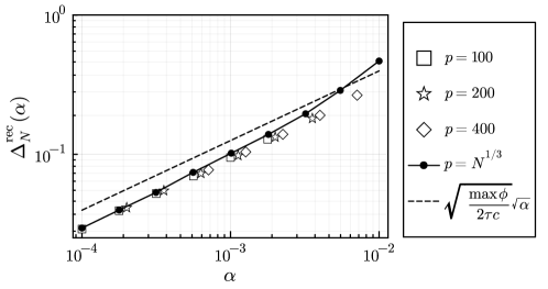
Figure 2: Large $N$ simulations of the distance $\Delta^{\mathrm{rec}}_{N}(\alpha)$ as a function of $\alpha$ for $p=100$ (rectangles), $p=200$ (stars), and $p=400$ (diamonds). Simulations of $\Delta^{\mathrm{rec}}_{N}(\alpha)$ for the duplicate-free sequence of networks $p=N^{1/3}$ (full circles). Theoretical $\mathcal{O}(\sqrt{\alpha})$ bound predicated by the feedforward model simplification (dashed line). Same parameters as in Fig. 1B-E.

(I) Large networks are duplicate-free.— Assuming that the bound (10) is tight for $C^{\mathrm{rec}}_{ij}$, for any distinct pair of units $i\neq j$, we have, by the central limit theorem, that the scaled correlation $\sqrt{p}\,C^{\mathrm{rec}}_{ij}$ converges in law to a standard normal random variable as $p\to\infty$. Then, if $p\to\infty$ as $N\to\infty$, we can prove that the distribution of correlations $\{C^{\mathrm{rec}}_{ij}\}_{i<j}$ converges to a centered normal distribution with variance $1/p$ as $N\to\infty$ (Fig. 1C; proof in ). More importantly, using the bound (10) and the fact that, for all $N,p>1$, it follows a Gegenbauer distribution with parameter $p$ (11), we can derive a bound for the probability of a duplicate:

$$\mathbb{P}(\exists\,i\neq j\text{ s.t. }|C_{ij}|\geq\varepsilon)\leq\frac{N(N-1)}{2}\frac{(1-\varepsilon^{2})^{\frac{p-1}{2}}}{\sqrt{\pi}},$$ (12)

for all $0<\varepsilon<1$ . Since we have $p=\alpha N$, the bound tends to $0$ as $N\to\infty$, which confirms that large networks are duplicate-free.

(II) Large SNNs converge to large RNNs at rate $\sqrt{\alpha}$, as $\alpha\to 0$.— For any fixed load $\alpha$, we define the average distance between the SNN and the RNN as

$$\Delta^{\mathrm{rec}}_{N}(\alpha)\mathrel{\mathop{\mathchar 58\relax}}=\frac{2}{N}\sum_{i=N/2+1}^{N}\lim_{T\to\infty}\frac{1}{T}\int_{0}^{T}\left|h^{\mathrm{rec}}_{i}(t)-x^{\mathrm{rec}}_{i}(t)\right|\mathrm{d}t$$

and the large $N$ limit distance as $\Delta^{\mathrm{rec}}(\alpha)\mathrel{\mathop{\mathchar 58\relax}}=\lim_{N\to\infty}\Delta^{\mathrm{rec}}_{N}(\alpha)$. Numerical estimates of the limit distance $\Delta^{\mathrm{rec}}(\alpha)$ as a function of $\alpha$ indicates that

$$\Delta^{\mathrm{rec}}(\alpha)=\mathcal{O}(\sqrt{\alpha}),\quad\text{as }\alpha\to 0$$ (13)

(Fig. 2). This scaling implies that large SNNs can converge to equally large RNNs despite the fact that (i) there is no duplicate averaging (Fig. 1C and (12)) and (ii) no temporal averaging (3). For example, if we take the sublinear scaling $p=N^{1/3}$, which implies $\alpha=N^{-2/3}$, the distance $\Delta^{\mathrm{rec}}_{N}(\alpha)\to 0$ vanishes (Fig. 2, full circles) and networks are duplicate-free (12), as $N\to\infty$.

In the absence of averaging of types (i) and (ii), the concentration of measure phenomenon [Tal96, Led01] can explain the convergence of SNNs to RNNs. In our case, the concentration of measure is controlled by the $\ell^{2}$ norm $\|\mathbf{J}_{i}\|_{2}=\sqrt{\sum_{j=1}^{N}J_{ij}^{2}}$ of each neuron $i$’s incoming weights. When $p=\alpha N$, for a typical neuron $i$, we find the convergence in probability

$$\|\mathbf{J}_{i}\|_{2}\xrightarrow[N\to\infty]{\mathbb{P}}\sqrt{\frac{\alpha}{c}},$$ (14)

(proof in ) which means that the $\ell^{2}$ norms of each neuron’s incoming weights concentrate around $\sqrt{\alpha/c}$ (where $c$ is defined after (7)). The numerical scaling (13) of the limit distance between large SNNs and large RNNs, as $\alpha\to 0$, corresponds to the theory-based scaling (14) of the limit $\ell^{2}$ norm of a typical neuron’s incoming weights.

Although we do not have an exact theory linking the limit $\ell^{2}$ norm (14) with the limit distance $\Delta^{\mathrm{rec}}(\alpha)$ (13), a simplified feedforward model, which is analytically tractable, offers a good intuition for the concentration of measure phenomenon at play. This simplified model is obtained by keeping network connections from ‘in’ to ‘rec’ neurons and removing all the other connections (Fig. 3).

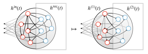
Figure 3: The feedforward model as a simplification of the input-driven model. Dotted lines indicate removed connections

After this pruning procedure, we are left with two-layer feedforward networks where the ‘in’ neurons make up the first layer, $(h^{\mathrm{in}}_{i}(t),x^{\mathrm{in}}_{i}(t))\mapsto(h^{(1)}_{i}(t),x^{(1)}_{i}(t))$, and the ‘rec’ neurons make up the second layer, $(h^{\mathrm{rec}}_{i}(t),x^{\mathrm{rec}}_{i}(t))\mapsto(h^{(2)}_{i}(t),x^{(2)}_{i}(t))$. In general, for any $N>1$ and for any connectivity matrix $\mathbf{J}$, we find that, for any neuron $i$ in the second layer, the single-neuron distance satisfies the bound

$$\lim_{T\to\infty}\frac{1}{T}\int_{0}^{T}\left|h^{(2)}_{i}(t)-x^{(2)}_{i}(t)\right|\mathrm{d}t\leq\sqrt{\frac{\max\phi}{2\tau}}\|\mathbf{J}_{i}\|_{2},$$

(proof in ) which is indeed controlled by the $\ell^{2}$ norm $\|\mathbf{J}_{i}\|_{2}$. Then, if $p=\alpha N$, using the convergence of the $\ell^{2}$ norm (14), we get the expected scaling for the limit distance, as $N\to\infty$, between a spiking neuron $h^{(2)}_{i}$ and a rate unit $x^{(2)}_{i}$:

$$\lim_{T\to\infty}\frac{1}{T}\int_{0}^{T}\left|h^{(2)}_{i}(t)-x^{(2)}_{i}(t)\right|\mathrm{d}t\leq\sqrt{\frac{\max\phi}{2\tau c}}\sqrt{\alpha}$$

(cf. Fig. 2). Therefore, the feedforward model provides an intuition for how the vanishing $\ell^{2}$ norms of the incoming weights (as $\alpha\to 0$) cause concentration of measure in duplicate-free, large SNNs. An exact theory of the original recurrent networks would require a full-fledged dynamical mean-field theory [HelDah20] for our input-driven disordered network model, which remains an open problem.

Concentration of measure [Led01] has been shown to be instrumental for the theory of spin glasses [Tal10] and the theory of infinite-width artificial neural networks [MeiMon22]. By contrast, this probabilistic notion has barely permeated the theory of large networks of spiking neurons. The standard perspective has been that, to produce spike-noise robust population dynamics, large networks have to perform averages over the spike activity of many neuronal duplicates [ShaNew98, GerKis02, GerKis14, Bre15], i.e. mechanism (i). Recently, DepSus23 argued, through extensive numerical simulations, that “weighted averages” over heterogeneous neurons could lead to population-level latent factors with noise-robust dynamics, which can then produce the illusion of rate-based dynamics. Our work provides a theoretical foundation for this idea as we show how the concentration of measure phenomenon can explain spike noise absorption in heterogeneous networks and the resulting emergence of (illusory) rate-based dynamics. This sheds new light on the long-standing debate about the mechanistic interpretability of rate-based theories in neuroscience [ShaNew98, GerKis02, GerKis14, Bre15, DepSus23].