M-Representation of Polytopes

Abstract We introduce the M-representation of polytopes, which makes it possible to compute linear transformations, convex hulls, and Minkowski sums with linear complexity in the dimension of the polytopes. When the polytope is a convex hull of a zonotope and a polytope, the representation size can be smaller than any of the known representations (V-representation, H-representation, and Z-representation). We also provide a variant of the M-representation: The chain representation is more compact and we can directly use it to compute linear transformations and convex hulls – for all other operations on the chain representation, one requires a conversion to the M-representation.

1 Introduction

The two main representations for convex, bounded polytopes are the well known V-representation and H-representation [7, 15]. The first one represents a polytope by its vertices and the second one uses halfspaces. Recently, the novel Z-representation was introduced in [10], which uses generators multiplied by monomials. The Z-representation is a special case of polynomial zonotopes [1], which can represent non-convex sets.

The Z-representation overcomes several shortcomings of the conventional representations, out of which we provide a few examples: In case the matrix $M$ of a linear transformation of an H-representation is not invertible, the computational complexity of this transformation is exponential in the dimension $d$ [8]. The complexity of calculating the Minkowski sum of two polytopes in H-representation is also exponential in $d$ [14] and the computation of the convex hull of two H-representations is NP-hard [14]. While the linear transformation of the V-representation is trivial, the computation of the Minkowski sum [6] and the convex hull [14] of two polytopes in V-representation are exponential in $d$. Contrary, the Z-representation has only a polynomial complexity for linear transformations, Minkowski sums and convex hulls with respect to the dimension $d$ [10].

Let us have a look at related representation types, which are also surveyed in [3]. The complexities are described in terms of the number of respective generators of these methods if not stated otherwise. Another representation for polytopes are zonotope bundles. This method presents polytopes as the intersection of a finite number of zonotopes [2]. An advantage of this method is that the intersection of two zonotope bundles can be found trivially, but neither the Minkowski sum, nor the convex hull have a closed-form expression [3]. Polynomial zonotopes [1] have a polynomial complexity for the Minkowski sum and the convex hull, but are not closed under intersections [3]. Besides polynomial zonotopes there also exist constrained zonotopes [13] and constrained polynomial zonotopes [9]. These have additional constraints on the factors appearing in the definition of a (polynomial) zonotope. The Minkowski sum can be computed in linear complexity for constrained (polynomial) zonotopes. While convex hulls of constrained polynomial zonotopes can be computed with polynomial complexity [3], convex hulls of constrained zonotopes can be computed linearly in the number of generators and constraints on the zonotopes [12]. Another representation are support functions [5]. Introduced by Minkowski it makes use of the supremum of an inner product. The Minkowski sum and the convex hull can be computed linearly, but the computation of intersections of support functions is not solved yet [3]. Spectrahedra are another way to represent convex sets. A spectrahedron is defined by the positive semi-definite values of a Hermitian linear matrix polynomial. Their representation by matrix polynomials makes them useful in linear programming [11].

As the main result of this paper, we introduce the M-representation for polytopes. Its form is similar to the Z-representation, but we constrain the factors to positive values. This rather subtle change has significant implications and improves many characteristics of the Z-representation: So far, we can only find a Z-representation whose number of generators is quadratic in the number of vertices $n$. The M-representation on the other hand only needs at most as many basis vectors as the V-representation and an additional matrix of exponents. This matrix can be saved efficiently such that it vanishes in the complexity of the representation size of the basis vectors. Furthermore, we introduce a strategy that uses zonotopes in order to decrease the number of basis vectors even further. Given $n$ vertices in $\mathbb{R}^{d}$ an M-representation can be computed in $\mathcal{O}(dn)$.

This paper is organized as follows: In Sec. 2 we present preliminaries and continue in Sec. 3 by introducing the M-representation. We prove the complexities of different operations in Sec. 4 and present an algorithm to reduce the number of basis vectors in Sec. 5. In Sec. 6 we propose a variant that reduces the complexity of computations convex hulls.

2 Preliminaries

2.1 Notations

In the remainder of this paper, we will use the following notations: $[n]=\{1,2,\dots,n\}$ for $n\in\mathbb{N}$, the symbols $\mathbb{O}$ and $\mathbb{I}$ refer to the matrices filled with zeros and ones with proper dimensions. $I_{n}$ refers to the identity matrix in $\mathbb{R}^{n\times n}$, $L_{n}$ to the lower triangular matrix filled with ones in $\mathbb{R}^{n\times n}$ and $[\textrm{ }]$ denotes the empty matrix. Given a matrix $M\in\mathbb{R}^{d\times d}$, $M_{(i,j)}$ represents the $j$-th entry of matrix row $i$, and $M_{(\cdot,j)}$ the $j$-th column. Furthermore, we will denote a set of the form $\{S(\alpha)\textrm{ }|\textrm{ }\alpha\in[0,1]^{p}\}$ as $\{S(\alpha)\}_{\alpha}$.

2.2 Definitions

Now we provide some definitions that are important for the rest of the paper. In order to make the paper coherent, we will use the term polytope instead of convex bounded polytope. Let us first define the V-representation, and the H-representation of polytopes.

Definition 2.1 (V-representation).

Let $v_{1},v_{2},\dots,v_{n}\in\mathbb{R}^{d}$ be the vertices of a polytope $\mathcal{P}$. Then we can define the vertex representation as

$$\mathcal{P}=\Big{\{}\sum_{i=1}^{n}\alpha_{i}v_{i}\textrm{ }\Big{|}\textrm{ }\sum_{i=1}^{n}\alpha_{i}=1,\alpha_{i}\geq 0\Big{\}}.$$ (1)

This representation therefore uses $n$ vectors.

Definition 2.2 (H-representation).

Let $G\in\mathbb{R}^{h\times d}$ be a matrix and $b\in\mathbb{R}^{h}$ a vector. The halfspace representation of a polytope $\mathcal{P}\subseteq\mathbb{R}^{d}$ is

$$\mathcal{P}=\{x\in\mathbb{R}^{d}\textrm{ }|\textrm{ }Gx\leq b\}.$$ (2)

This representation uses $h$ halfspaces.

Let us now define the Z-representation of a polytope, which is a special case of a polynomial zonotope.

Definition 2.3 (Z-representation).

Let $c\in\mathbb{R}^{d}$ be a center point, $G\in\mathbb{R}^{d\times h}$ a generator matrix, and $\mathcal{E}\in\{0,1\}^{p\times h}$ an exponent matrix, then the Z-representation of a polytope $\mathcal{P}\subseteq\mathbb{R}^{d}$ is defined as

$$\mathcal{P}=\Big{\{}c+\sum_{i=1}^{h}(\prod_{k=1}^{p}\alpha_{k}^{\mathcal{E}_{(k,i)}})G_{(\cdot,i)}\textrm{ }\Big{|}\textrm{ }\alpha\in[-1,1]^{p}\Big{\}}$$ (3)

and we write

$$\mathcal{P}=\langle c,G,\mathcal{E}\rangle_{Z}.$$ (4)

The Z-representation of a single point $c$ therefore can be expressed by $\langle c,[\textrm{ }],[\textrm{ }]\rangle_{Z}$. This representation uses $h$ generators.

The Z-representation is not unique. For example, the polytope in Fig. 1 can be represented by the following two sets $\mathcal{P}_{1}$ and $\mathcal{P}_{2}$ with $\mathcal{P}_{1}=\mathcal{P}_{2}$.

$$\begin{split}\mathcal{P}_{1}&=\Big{\langle}\begin{pmatrix}0\\ 0\end{pmatrix},\Big{[}\begin{pmatrix}1\\ 0\end{pmatrix},\begin{pmatrix}-1\\ -1\end{pmatrix}\Big{]},\begin{pmatrix}10\\ 01\end{pmatrix}\Big{\rangle}_{Z}\\ \mathcal{P}_{2}&=\Big{\langle}\begin{pmatrix}0\\ 0\end{pmatrix},\Big{[}\begin{pmatrix}-0.5\\ -0.5\end{pmatrix},\begin{pmatrix}-0.5\\ -0.5\end{pmatrix},\begin{pmatrix}0.5\\ 0\end{pmatrix},\begin{pmatrix}-0.5\\ -0.5\end{pmatrix},\begin{pmatrix}0.5\\ 0.5\end{pmatrix}\Big{]},\begin{pmatrix}10010\\ 01001\\ 00111\end{pmatrix}\Big{\rangle}_{Z}\end{split}$$ (5)

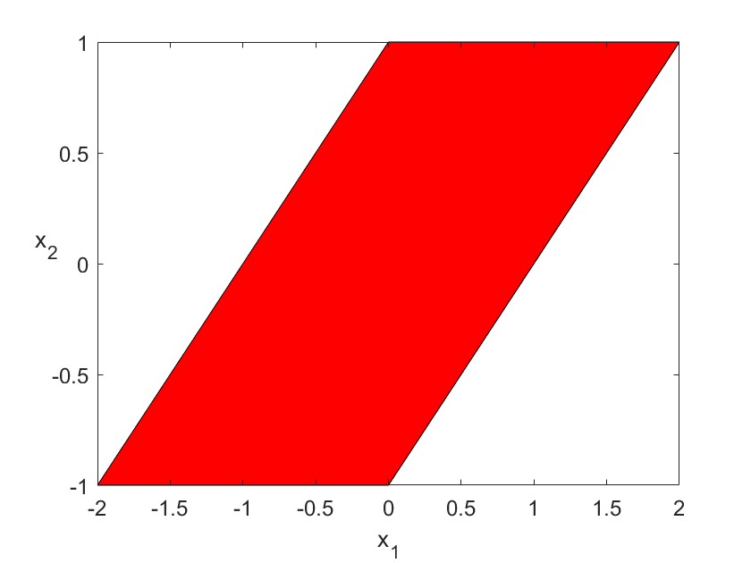
Figure 1: Plot of $\mathcal{P}_{1}=\mathcal{P}_{2}$

Let us now have a look at zonotopes. The set of zonotopes is a subset of the set of polytopes, we can therefore express zonotopes as a special case of polytopes in Z-representation:

Definition 2.4 (Zonotope).

A zonotope is a polytope in Z-representation with $\mathcal{E}=I_{h}$.

Definition 2.5 (Convex hull, Minkowski sum).

Let $\mathcal{P}_{1}$ and $\mathcal{P}_{2}$ be two convex sets. Then we define the convex hull as

$$conv(\mathcal{P}_{1},\mathcal{P}_{2})=\Big{\{}\frac{1+\alpha}{2}p_{1}+\frac{1-\alpha}{2}p_{2}\textrm{ }\Big{|}\textrm{ }p_{1}\in\mathcal{P}_{1},p_{2}\in\mathcal{P}_{2},\alpha\in[-1,1]\Big{\}}$$ (6)

and the Minkowski sum as

$$\mathcal{P}_{1}\oplus\mathcal{P}_{2}=\Big{\{}p_{1}+p_{2}\textrm{ }\Big{|}\textrm{ }p_{1}\in\mathcal{P}_{1},\textrm{ }p_{2}\in\mathcal{P}_{2}\Big{\}}.$$ (7)

The convex hull and the Minkowski sum of two polytopes can be computed in the following way:

Proposition 2.6 (Convex hull, Minkowski sum, Linear transformation, [10]).

Let $\mathcal{P}_{1}$ and $\mathcal{P}_{2}$ be two polytopes in Z-representation with $\mathcal{P}_{i}=\langle c_{i},G_{i},\mathcal{E}_{i}\rangle_{Z}$, $c_{i}\in\mathbb{R}^{d}$, $G_{i}\in\mathbb{R}^{d\times h_{i}}$ and $\mathcal{E}_{i}\in\{0,1\}^{p_{i}\times h_{i}}$. Then their convex hull and Minkowski sum can be computed by

$$\begin{split}conv(\mathcal{P}_{1},\mathcal{P}_{2})&=\Big{\langle}\frac{1}{2}(c_{1}+c_{2}),\frac{1}{2}[(c_{1}-c_{2}),G_{1},G_{1},G_{2},-G_{2}],\hat{\mathcal{E}}\Big{\rangle}_{Z}\\ \mathcal{P}_{1}\oplus\mathcal{P}_{2}&=\Big{\langle}c_{1}+c_{2},[G_{1},G_{2}],\bar{\mathcal{E}}\Big{\rangle}_{Z}\end{split}$$ (8)

with

$$\begin{split}\hat{\mathcal{E}}&=\begin{pmatrix}\mathbb{O}&\mathcal{E}_{1}&\mathcal{E}_{1}&\mathbb{O}&\mathbb{O}\\ \mathbb{O}&\mathbb{O}&\mathbb{O}&\mathcal{E}_{2}&\mathcal{E}_{2}\\ 1&\mathbb{O}&\mathbb{I}&\mathbb{O}&\mathbb{I}\end{pmatrix}\\ \bar{\mathcal{E}}&=\begin{pmatrix}\mathcal{E}_{1}&\mathbb{O}\\ \mathbb{O}&\mathcal{E}_{2}\end{pmatrix}\\ p&=p_{1}+p_{2}+1.\end{split}$$ (9)

For the convex hull we have $h=2h_{1}+2h_{2}+1$ generators and for the Minkowski sum $h=h_{1}+h_{2}$ generators.
A linear transformation by $M\in\mathbb{R}^{m\times d}$ can be computed by

$$M\mathcal{P}_{1}=\langle Mc_{1},MG_{1},\mathcal{E}_{1}\rangle_{Z}.$$ (10)

For our M-representation we need another definition:

Definition 2.7 (Multilinear map).

A multivariate map $f:\mathbb{R}^{h}\to\mathbb{R}^{d}$ is called multilinear if it is linear in every variable.

In the next section, we introduce our novel M-representation.

3 M-Representation

By limiting the intervals of the factors of the Z-representation to $[0,1]$ we obtain the M-representation. This subtle change has far-reaching consequences and combines the computational advantages of the Z-representation with the low representation size of the V-representation.

Definition 3.1 (M-representation).

Let $s\in\mathbb{R}^{d}$ be a starting point, $B\in\mathbb{R}^{d\times h}$ a matrix of basis vectors, and $\mathcal{E}\in\{0,1\}^{p\times h}$ a matrix of exponents, then the multilinear vertex representation (M-representation) of a polytope $\mathcal{P}\subseteq\mathbb{R}^{d}$ is defined as

$$\mathcal{P}=\Big{\{}s+\sum_{i=1}^{h}(\prod_{k=1}^{p}\alpha_{k}^{\mathcal{E}_{(k,i)}})B_{(\cdot,i)}\textrm{ }\Big{|}\textrm{ }\alpha\in[0,1]^{p}\Big{\}}$$ (11)

and we write

$$\mathcal{P}=\langle s,B,\mathcal{E}\rangle_{M}.$$ (12)

The M-representation of a single point $s$ therefore can be expressed by $\langle s,[\textrm{ }],[\textrm{ }]\rangle_{M}$.

Now we introduce a theorem that provides a strategy to obtain an M-representation from a set of vertices. Furthermore, we prove how many basis vectors are at most required to represent a general polytope.

Theorem 3.2.

Let $v_{1},v_{2},\dots,v_{n}\in\mathbb{R}^{d}$ be the vertices of a polytope $\mathcal{P}$.

• We can express $\mathcal{P}$ in M-representation as

  $$\mathcal{P}=\langle v_{n},[v_{1}-v_{2},v_{2}-v_{3},\dots,v_{n-1}-v_{n}],L_{n-1}\rangle_{M}.$$ (13)

  This representation can be obtained with complexity $\mathcal{O}(nd)$ and has a representation size in $\mathcal{O}(nd)$.

• This representation has $h=n-1$ basis vectors.

We call this form the chain form.

Proof.

We prove the statements above by induction.

Induction start: The M-representation of a polytope with a single vertex $v$ is $\mathcal{P}=\langle v,[\textrm{ }],[\textrm{ }]\rangle_{M}=v$ with zero basis vectors. We can compute the convex hull of two vertices $v_{1},v_{2}$ as

$$conv(v_{1},v_{2})=\{\alpha v_{1}+(1-\alpha)v_{2}\}_{\alpha}=\{v_{2}+\alpha(v_{1}-v_{2})\}_{\alpha}$$ (14)

with one basis vector $v_{1}-v_{2}$. Therefore, $h(1)=0$ and $h(2)=1$. For $n\leq 2$, these representations have the form described in the theorem.

Induction step: Let $\mathcal{P}_{1}$ and $\mathcal{P}_{2}$ be two polytopes in M-representation. From

$$conv(\mathcal{P}_{1},\mathcal{P}_{2})=\{\alpha\cdot p_{1}+(1-\alpha)\cdot p_{2}\textrm{ }|\textrm{ }p_{1}\in\mathcal{P}_{1},\textrm{ }p_{2}\in\mathcal{P}_{2},\textrm{ }\alpha\in[0,1]\}$$ (15)

we know that $h(n)=h(n_{1})+2h(n_{2})+1$ with $n=n_{1}+n_{2}$ and $n_{i}$ is the number of vertices of the polytopes being merged in this step.
With $h(m)=m-1$ for every $m\in[n]$ and the claim of induction, it is obvious that a polytope with $n+1$ vertices has the least number of generators if we choose $n_{1}=n$ and $n_{2}=1$. Then we obtain $h(n+1)=n-1+2\cdot 0+1=n$, which proves the second part of the theorem. For the first part, we need the representation of a polytope $\mathcal{P}_{n}$ with $n$ vertices in order to compute the induction step. For this polytope we use

$$\mathcal{P}_{n}=\Big{\{}v_{n}+\sum_{i=1}^{n-1}\Big{(}\prod_{j=1}^{n-i}\alpha_{n-j}\Big{)}(v_{i}-v_{i+1})\Big{\}}_{\alpha}.$$ (16)

For the representation of a polytope $\mathcal{P}_{n+1}$ with $n+1$ vertices we obtain

$$\begin{split}\mathcal{P}_{n+1}&=conv(\mathcal{P}_{n},v_{n+1})=\\ \textrm{ }&=\Big{\{}\alpha_{n}\Big{(}v_{n}+\sum_{i=1}^{n-1}\Big{(}\prod_{j=1}^{n-i}\alpha_{n-j}\Big{)}(v_{i}-v_{i+1})\Big{)}+(1-\alpha_{n})v_{n+1}\Big{\}}_{\alpha}=\\ \textrm{ }&=\Big{\{}v_{n+1}+\sum_{i=1}^{n-1}\Big{(}\prod_{j=0}^{n-i}\alpha_{n-j}\Big{)}(v_{i}-v_{i+1})+\alpha_{n}(v_{n}-v_{n+1})\Big{\}}_{\alpha}=\\ \textrm{ }&=\Big{\{}v_{n+1}+\sum_{i=1}^{n}\Big{(}\prod_{j=0}^{n-i}\alpha_{n-j}\Big{)}(v_{i}-v_{i+1})\Big{\}}_{\alpha}=\\ \textrm{ }&=\Big{\{}v_{n+1}+\sum_{i=1}^{n}\Big{(}\prod_{k=1}^{n+1-i}\alpha_{n+1-k}\Big{)}(v_{i}-v_{i+1})\Big{\}}_{\alpha}=\\ \textrm{ }&=\langle v_{n+1},\textrm{ }[v_{1}-v_{2},v_{2}-v_{3},\dots,v_{n}-v_{n+1}],\textrm{ }L_{n}\rangle_{M}.\end{split}$$ (17)

In order to obtain this representation, $nd$ subtractions are necessary, therefore the complexity is in $\mathcal{O}(nd)$. For the representation size we only need to save the matrix of basis vectors and the index of the lower triangular matrix which leads to a complexity of $\mathcal{O}(nd)$. This proves the first part of the theorem. ∎

Let us have a look at why Theorem 3.2 cannot be adapted for the Z-representation:

Corollary 3.3.

A Z-representation of a polytope of the following form is always a point symmetric polytope:

$$\mathcal{P}=\langle c,[v_{1},v_{2},\dots,v_{n-1}],L_{n-1}\rangle_{Z}.$$ (18)

Proof.

Let $\mathcal{P}$ be defined as above. Then

$$\mathcal{P}=\Big{\{}c+\sum_{i=1}^{n-1}\Big{(}\prod_{j=1}^{n-i}\alpha_{n-j}\Big{)}v_{i}\textrm{ }\Big{|}\textrm{ }\alpha\in[-1,1]^{n-1}\Big{\}}.$$ (19)

From the Z-representation we know that the vertices are the points of this set with $\alpha_{i}\in\{-1,1\}$. Let $c+w$ be a vertex of $\mathcal{P}$ with $\alpha_{n-1}=1$. Then by (19) follows that $c-w$ is also a vertex of $\mathcal{P}$ if we only replace $\alpha_{n-1}=-1$. Therefore, each vertex has a partner which is point symmetric to the center $c$. ∎

From this we know that a general polytope with $n$ vertices cannot be represented by a Z-representation of the form in (18) with $n-1$ generators. In Proposition 4.2 we prove another advantage of the M-representation over the Z-representation even if there exist representations of polytopes with the same number of generators/basis vectors.

The next corollary follows directly from the theorem above as well:

Corollary 3.4.

Let $\mathcal{P}$ be a polytope of the form introduced in Theorem 3.2. Let $\alpha$ and $\alpha^{\prime}$ represent two points in a polytope and let $k$ be maximal s.t. $\alpha_{k}=0$. In case there is no such $k$, set $k=1$. Then $\alpha$ and $\alpha^{\prime}$ represent the same point iff $\alpha_{j}=\alpha^{\prime}_{j}$ for all $k\leq j\leq n-1$.

Example 3.5.

This means that for a polytope in the form of Theorem 3.2 with three basis vectors, all $\alpha$’s of the form $\alpha=\begin{pmatrix}\alpha_{1}\\ 0\\ 1\end{pmatrix}$ represent the same point in the polytope.

For a polytope $\mathcal{P}$ in the form of Theorem 3.2, the vertices can be computed by all combinations of the $\alpha_{i}\in\{0,1\}$. With Corollary 3.4 the vertices of $\mathcal{P}$ can be represented by the $\alpha$’s of the form of the columns of $L_{n-1}$ and the zero vector. From Theorem 3.2 it is clear that we can recover the vertices iteratively in $\mathcal{O}(nd)$ operations.

Remark.

If we define the starting point of the M-representation as a basis vector as well, this representation has the same number of basis vectors for general polytopes as the V-representation has vertices.

Proposition 3.6.

Obtaining a chain form of a general polytope $\mathcal{P}$ in M-representation with $h$ basis vectors and $p$ factors can be done in $\mathcal{O}(2^{p}hd)$.

Proof.

In order to obtain a chain form of a polytope $\mathcal{P}$ in M-representation, we need to compute the $2^{p}$ potential vertices of $\mathcal{P}$. In general this can be done in $\mathcal{O}(2^{p}hd)$. From Theorem 3.2 we know that we can obtain the chain form of these vertices in $\mathcal{O}(2^{p}d)$. ∎

4 Operations on Polytopes in M-Representation

In this section we present the linear transformation, Minkowski sum, and convex hull of polytopes in M-representation.

Theorem 4.1.

The M-representation of a polytope $\mathcal{P}=\langle s,B,\mathcal{E}\rangle_{M}$ in $\mathbb{R}^{d}$ with $h$ basis vectors directly inherits the efficient computation of linear transformations and Minkowski sums from the Z-representation. A linear transformation by $M\in\mathbb{R}^{m\times d}$ can be computed as

$$M\mathcal{P}=\langle Ms,MB,\mathcal{E}\rangle_{M}.$$ (20)

This can be done in $\mathcal{O}(mdh)$.
The Minkowski sum of two polytopes $\mathcal{P}_{1}=\langle s_{1},B_{1},\mathcal{E}_{1}\rangle_{M}$ and $\mathcal{P}_{2}=\langle s_{2},B_{2},\mathcal{E}_{2}\rangle_{M}$ can be computed as

$$\mathcal{P}_{1}\oplus\mathcal{P}_{2}=\Big{\langle}s_{1}+s_{2},[B_{1},B_{2}],\begin{pmatrix}\mathcal{E}_{1}&\mathbb{O}\\ \mathbb{O}&\mathcal{E}_{2}\end{pmatrix}\Big{\rangle}_{M}.$$ (21)

This can be computed in $\mathcal{O}(d)$ and the representation size is in $\mathcal{O}\Big{(}(h_{1}+h_{2})\cdot max\{h_{1}+h_{2},d\}\Big{)}$.
If $\mathcal{P}_{1}$ and $\mathcal{P}_{2}$ are in chain form, the matrix of exponents can be represented as $\begin{pmatrix}L_{h_{1}}&\mathbb{O}\\ \mathbb{O}&L_{h_{2}}\end{pmatrix}$. This has a representation size in $\mathcal{O}\Big{(}(h_{1}+h_{2})d\Big{)}$.

Proof.

The proof is identical to the one for the Z-representation in [10] since all operations are independent of the range of the factors $\alpha_{i}$. For the representation of polytopes in chain form we only need to save the matrix of basis vectors and a $2\times 2$ matrix filled with the indices of the lower triangular matrices and the $\mathbb{O}$ symbol. Therefore the representation size is in $\mathcal{O}\Big{(}(h_{1}+h_{2})d\Big{)}$. ∎

In [6] the number of vertices for the Minkowski sum of $k$ polytopes in $\mathbb{R}^{d}$ is discussed. If each of the polytopes has at most $n$ vertices, the total number of vertices is in $\mathcal{O}(k^{d-1}n^{2(d-1)})$.
From Theorem 4.1 follows that the number of basis vectors of $k$ polytopes is the sum of the number of basis vectors of each polytope. Let each polytope be represented by at most $n$ basis vectors, i.e. the polytope has at least $n$ vertices if we use the representation from Theorem 3.2. Then the number of basis vectors of the Minkowski sum of these polytopes is in $\mathcal{O}(kn)$.

Let $\mathcal{P}_{M1}$ and $\mathcal{P}_{M2}$ be two polytopes in M-representation with $h_{M}$ basis vectors each, $\mathcal{P}_{Z1}$ and $\mathcal{P}_{Z2}$ be two polytopes in Z-representation with $h_{Z}$ generators each and $h_{Z}=h_{M}$. Then $conv(\mathcal{P}_{M1},\mathcal{P}_{M2})$ needs $h_{M}$ basis vectors less than $conv(\mathcal{P}_{Z1},\mathcal{P}_{Z2})$ needs generators:

Proposition 4.2.

Let $\mathcal{P}_{1}=\langle s_{1},B_{1},\mathcal{E}_{1}\rangle_{M}$ and $\mathcal{P}_{2}=\langle s_{2},B_{2},\mathcal{E}_{2}\rangle_{M}$ be two polytopes in M-representation with $h_{1}\geq h_{2}$ being the respective number of basis vectors. Then

$$\begin{split}\mathcal{P}&=conv(\mathcal{P}_{1},\mathcal{P}_{2})=\langle s_{2},[B_{2},-B_{2},B_{1},s_{1}-s_{2}],\mathcal{E}\rangle_{M},\end{split}$$ (22)

with

$$\mathcal{E}=\begin{pmatrix}\mathcal{E}_{2}&\mathcal{E}_{2}&\mathbb{O}&\mathbb{O}\\ \mathbb{O}&\mathbb{O}&\mathcal{E}_{1}&\mathbb{O}\\ \mathbb{O}&\mathbb{I}&\mathbb{I}&1\end{pmatrix}$$ (23)

being a block matrix and $\mathcal{P}$ has $h=h_{1}+2h_{2}+1$ basis vectors. The complexity of obtaining the convex hull of two polytopes in M-representation is in $\mathcal{O}(d)$ and the representation size is in $\mathcal{O}\Big{(}max\Big{\{}(h_{1}+2h_{2}+1)d,(h_{1}+h_{2}+1)^{2}\Big{\}}\Big{)}$.
If $\mathcal{P}_{1}$ and $\mathcal{P}_{2}$ are in chain form, the matrix of exponents can be represented as

$$\mathcal{E}=\begin{pmatrix}L_{h_{2}}&L_{h_{2}}&\mathbb{O}&\mathbb{O}\\ \mathbb{O}&\mathbb{O}&L_{h_{1}}&\mathbb{O}\\ \mathbb{O}&\mathbb{I}&\mathbb{I}&1\end{pmatrix}.$$ (24)

This has a representation size in $\mathcal{O}\Big{(}(h_{1}+2h_{2}+1)d\Big{)}$.

Proof.

We write two polytopes $\mathcal{P}_{1}=\langle v_{n},B_{1},\mathcal{E}_{1}\rangle_{M}$ and $\mathcal{P}_{2}=\langle w_{m},B_{2},\mathcal{E}_{2}\rangle_{M}$ as $\mathcal{P}_{1}=\Big{\{}v_{n}+\sum_{i=1}^{n-1}\Big{(}\prod_{j=1}^{n-i}\alpha_{n-j}\Big{)}(v_{i}-v_{i+1})\Big{\}}_{\alpha}$ and $\mathcal{P}_{2}=\Big{\{}w_{m}+\sum_{i=1}^{m-1}\Big{(}\prod_{j=1}^{m-i}\alpha_{m-j}\Big{)}(w_{i}-w_{i+1})\Big{\}}_{\alpha}$ with $n-1$ and $m-1$ basis vectors, respectively. Then

$$\begin{split}\mathcal{P}&=conv(\mathcal{P}_{1},\mathcal{P}_{2})=\\ \textrm{ }&=\Big{\{}\alpha_{n+m-1}\Big{(}v_{n}+\sum_{i=1}^{n-1}\Big{(}\prod_{j=1}^{n-i}\alpha_{n-j}\Big{)}(v_{i}-v_{i+1})\Big{)}+\\ \textrm{ }&+(1-\alpha_{n+m-1})\Big{(}w_{m}+\sum_{i=1}^{m-1}\Big{(}\prod_{j=1}^{m-i}\alpha_{m-j}\Big{)}(w_{i}-w_{i+1})\Big{)}\Big{\}}_{\alpha}=\\ \textrm{ }&=\Big{\{}w_{m}+\sum_{i=1}^{m-1}\Big{(}\prod_{j=1}^{m-i}\alpha_{m-j}\Big{)}(w_{i}-w_{i+1})+\alpha_{n+m-1}\Big{(}-\sum_{i=1}^{m-1}\Big{(}\prod_{j=1}^{m-i}\alpha_{m-j}\Big{)}(w_{i}-w_{i+1})\Big{)}+\\ \textrm{ }&+\alpha_{n+m-1}\Big{(}\sum_{i=1}^{n-1}\Big{(}\prod_{j=1}^{n-i}\alpha_{n-j}\Big{)}(v_{i}-v_{i+1})\Big{)}+\alpha_{n+m-1}(v_{n}-w_{m})\Big{\}}_{\alpha}=\\ \textrm{ }&=\langle w_{m},[G_{2},-G_{2},G_{1},v_{n}-w_{m}],\mathcal{E}\rangle_{M}\end{split}$$ (25)

with $\mathcal{E}$ as defined above.
For the representation of polytopes in chain form we only need to save the matrix of basis vectors and a $3\times 4$ matrix filled with the indices of the lower triangular matrices, the symbols $\mathbb{O}$ and $\mathbb{I}$ and a 1. Therefore the representation size is in $\mathcal{O}\Big{(}(h_{1}+2h_{2}+1)d\Big{)}$. ∎

A more compact representation of $conv(\mathcal{P}_{1},\mathcal{P}_{2})$ in terms of number of basis vectors can be obtained by computing the vertices of $\mathcal{P}_{1}$ and $\mathcal{P}_{2}$, deleting the ones that are not vertices of the convex hull of $\mathcal{P}_{1}$ and $\mathcal{P}_{2}$, and using the strategy from Theorem 3.2 to obtain the M-representation of the remaining vertices. This method would result in a maximum of $h=n_{1}+n_{2}-1=h_{1}+h_{2}+1$ basis vectors. However, the computational complexity of deleting the vertices that are not vertices of the convex hull has exponential complexity in the number $d$ of dimensions, similar to the computation of the convex hull of two polytopes in V-representation [14]. In order to reduce the representation size of the convex hull for polytopes in chain form, we introduce a variant of the M-representation in Sec. 6.

5 Algorithm for Reducing the Number of Basis Vectors in M-Representation

Now we want to introduce an algorithm that returns an M-representation with at most $n-1$ basis vectors for a polytope with $n$ vertices. In case the vertices of the polytope fulfill certain condidtions, this algorithm returns less than $n-1$ basis vectors. Let us have a closer look at zonotopes in M-representation for this. From [6] we know that zonotopes are Minkowski sums of line segments. We can use this for the M-representation of zonotopes.

Proposition 5.1.

Let $\mathcal{Z}$ be an $m$-dimensional zonotope in $\mathbb{R}^{d}$ with $n$ vertices which is spanned by the Minkowski sum of $h$ line segments. Let the line segments be of the form $[l_{i1},l_{i2}]$ with $i\in[h]$, where $l_{i1}$ is the starting point and $l_{i2}$ is the end point of this line segment. Then we can express $\mathcal{Z}$ as

$$\mathcal{Z}=\Big{\langle}\sum_{i=1}^{h}l_{i1},[l_{12}-l_{11},l_{22}-l_{21},\dots,l_{h2}-l_{h1}],I_{h}\Big{\rangle}_{M}.$$

This representation uses $h$ basis vectors.

Proof.

We can represent each line segment $l_{i}$ by

$$l_{i}=\langle l_{i1},[l_{i2}-l_{i1}],1\rangle_{M}.$$ (26)

By applying Theorem 4.1 $h-1$ times, we obtain the stated result with $h$ basis vectors. ∎

Lemma 5.2.

Let $\mathcal{Z}$ be an $m$-dimensional zonotope in $\mathbb{R}^{d}$ with $n$ vertices and $m,h\neq 0$. Then we can represent $\mathcal{Z}$ by at most $h\leq\frac{n}{2}$ pairwise distinct basis vectors in M-representation.

Proof.

For the cases with $m<2$ and $h<2$ this is clear. For all other cases we can use Proposition 2.1.2 in [6]: For an $m$-dimensional zonotope in $\mathbb{R}^{d}$ with $h$ pairwise distinct basis vectors in M-representation and $n$ vertices the following relation holds:

$$n=2\sum_{i=0}^{min\{m,h\}-1}\binom{h-1}{i}$$ (27)

From this, we obtain the following inequality:

$$n=2\sum_{i=0}^{min\{m,h\}-1}\binom{h-1}{i}\geq 2\binom{h-1}{0}+2\binom{h-1}{1}=2h$$ (28)

∎

Hence, we can represent every zonotope by less than $n-1$ basis vectors for $n>2$. We can use this to represent general polytopes, where a subset of the vertices forms a zonotope, by less than $n-1$ basis vectors. Alg. 1 returns at most $n-1$ basis vectors for general polytopes with $n$ vertices.

Input: Set $V$ containing $n$ vertices in $\mathbb{R}^{d}$

Output: M-representation of the polytope spanned by $V$ with at most $h=n-1$ basis vectors

if $\exists S\subseteq V$ s.t. $S$ spans a zonotope, $|S|>2$ and $S$ maximal then

       use Proposition 5.1 on $S$ and use Proposition 4.2 to add the vertices in $V\setminus S$ one by one to the representation of $S$

else

       use Theorem 3.2 on the vertex set $V$

end if

Algorithm 1 Algorithm for obtaining an M-representation

It is clear that this representation is multilinear again.
For checking whether a set is a zonotope we can use [4, Alg. 3], which introduces an algorithm for checking whether a set of vertices forms a zonotope. This algorithm also returns the line segments which span the zonotope by their Minkowski sum. In order to be able to represent this polytope by an M-representation, we still need to apply Proposition 5.1. As candidates for such a set $S$ as described in Alg. 1, we only need to take sets into account that are point symmetric to a center as this is a necessary criterion for a set to be a zonotope.
Now we look at an example of an application of Alg. 1 that reduces the number of basis vectors $h$ from 4 to 3 for 5 vertices.

Example 5.3.

Let $\mathcal{P}$ be a polytope with the 5 vertices $\begin{pmatrix}0\\ 0\end{pmatrix},\begin{pmatrix}0\\ 2\end{pmatrix},\begin{pmatrix}2\\ 2\end{pmatrix},\begin{pmatrix}2\\ 0\end{pmatrix},\begin{pmatrix}1\\ 3\end{pmatrix}$. The first four vertices form a zonotope that can be represented by

$$\mathcal{P}^{\prime}=\Big{\{}\begin{pmatrix}0\\ 0\end{pmatrix}+\alpha_{1}\cdot\begin{pmatrix}0\\ 2\end{pmatrix}+\alpha_{2}\cdot\begin{pmatrix}2\\ 0\end{pmatrix}\Big{\}}_{\alpha}.$$ (29)

$\mathcal{P}$ can be written in M-representation as

$$\begin{split}\mathcal{P}&=\Big{\{}\alpha_{3}\cdot\mathcal{P}^{\prime}+(1-\alpha_{3})\cdot\begin{pmatrix}1\\ 3\end{pmatrix}\Big{\}}_{\alpha}\\ &=\Big{\{}\begin{pmatrix}1\\ 3\end{pmatrix}+\alpha_{3}\cdot\begin{pmatrix}-1\\ -3\end{pmatrix}+\alpha_{1}\alpha_{3}\cdot\begin{pmatrix}0\\ 2\end{pmatrix}+\alpha_{2}\alpha_{3}\cdot\begin{pmatrix}2\\ 0\end{pmatrix}\Big{\}}_{\alpha},\end{split}$$ (30)

which has only 3 basis vectors.

Example 5.4.

Let us have a look at the polytope shown in Fig. 1. In M-representation, this polytope could be represented by

$$\begin{split}\mathcal{P}&=\Big{\langle}\begin{pmatrix}-2\\ -1\end{pmatrix},\Big{[}\begin{pmatrix}-2\\ -2\end{pmatrix},\begin{pmatrix}2\\ 0\end{pmatrix},\begin{pmatrix}2\\ 2\end{pmatrix}\Big{]},\begin{pmatrix}100\\ 110\\ 111\end{pmatrix}\Big{\rangle}_{M}=\\ \textrm{ }&=\Big{\{}\begin{pmatrix}-2\\ -1\end{pmatrix}+\alpha_{1}\alpha_{2}\alpha_{3}\cdot\begin{pmatrix}-2\\ -2\end{pmatrix}+\alpha_{2}\alpha_{3}\cdot\begin{pmatrix}2\\ 0\end{pmatrix}+\alpha_{3}\cdot\begin{pmatrix}2\\ 2\end{pmatrix}\Big{\}}_{\alpha}.\end{split}$$ (31)

If we apply Alg. 1, we can even express it as

$$\begin{split}\mathcal{P}&=\Big{\langle}\begin{pmatrix}-2\\ -1\end{pmatrix},\Big{[}\begin{pmatrix}2\\ 0\end{pmatrix},\begin{pmatrix}2\\ 2\end{pmatrix}\Big{]},\begin{pmatrix}10\\ 01\end{pmatrix}\Big{\rangle}_{M}=\\ \textrm{ }&=\Big{\{}\begin{pmatrix}-2\\ -1\end{pmatrix}+\alpha_{1}\cdot\begin{pmatrix}2\\ 0\end{pmatrix}+\alpha_{2}\cdot\begin{pmatrix}2\\ 2\end{pmatrix}\Big{\}}_{\alpha}.\end{split}$$ (32)

6 Chain Representation of the Chain Form

Now we introduce a variant of the M-representation, which makes it possible to reduce the computational complexity of the convex hull of two polytopes in $\mathbb{R}^{d}$ with $h$ basis vectors each and in chain form to $\mathcal{O}(d)$:

Definition 6.1.

Let $s\in\mathbb{R}^{d}$ be a starting point, $B\in\mathbb{R}^{d\times h}$ a matrix of basis vectors, $\mathcal{E}=L_{h}$ a matrix of exponents and $e\in\mathbb{R}^{d}$ an end point, then a chain representation (C-representation) of a polytope $\mathcal{P}\subseteq\mathbb{R}^{d}$ in chain form is defined as

$$\mathcal{P}=\Big{\{}s+\sum_{i=1}^{h}(\prod_{k=1}^{p}\alpha_{k}^{\mathcal{E}_{(k,i)}})B_{(\cdot,i)}\textrm{ }\Big{|}\textrm{ }\alpha\in[0,1]^{p}\Big{\}}$$ (33)

and we write

$$\mathcal{P}=\langle s,B,e\rangle_{C}.$$ (34)

The basis vectors appearing in $B$ connect the starting point and the end point, which looks like a chain. It is sufficient so save $s$, $B$ and $e$, since the exponent matrix in chain form is uniquely defined by the dimensions of $B$. This variant has a representation size in $\mathcal{O}(hd)$. Saving the end point helps us for the next proposition:

Proposition 6.2.

Let $\mathcal{P}_{1}=\langle s_{1},B_{1},e_{1}\rangle_{C}$ and $\mathcal{P}_{2}=\langle s_{2},B_{2},e_{2}\rangle_{C}$ be two polytopes in $\mathbb{R}^{d}$ in C-representation with $h_{1}$ and $h_{2}$ being the respective number of basis vectors. Then

$$\begin{split}\mathcal{P}&=conv(\mathcal{P}_{1},\mathcal{P}_{2})=\langle s_{1},[B_{1},s_{2}-e_{1},B_{2}],e_{2}\rangle_{C}\end{split}$$ (35)

and $\mathcal{P}$ has $h=h_{1}+h_{2}+1$ basis vectors. The complexity of obtaining the convex hull of two polytopes in C-representation is $\mathcal{O}(d)$ and can be represented in $\mathcal{O}(hd)$.

Proof.

The set of vertices of the convex hull of $\mathcal{P}_{1}$ and $\mathcal{P}_{2}$ is a subset of the union of the vertices of these polytopes. It is clear from the definition of the chain form, that (35) represents a polytope. From Theorem 3.2 also follows that the vertices of the polytope in (35) can be represented by $\alpha$’s of the form of the zero vector and the columns of a lower triangular matrix filled with ones with dimensions $(h_{1}+h_{2}+1)\times(h_{1}+h_{2}+1)$. The matrix of basis vectors is the connection of the original chains $B_{1}$ and $B_{2}$ by the link between the end point $e_{1}$ and the starting point $s_{2}$. This returns as vertices of the polytope $\mathcal{P}$ the union of the vertex sets of $\mathcal{P}_{1}$ and $\mathcal{P}_{2}$. Hence, (35) represents the required convex hull. ∎

Proposition 6.3.

The C-representation of a polytope $\mathcal{P}=\langle s,B,e\rangle_{C}$ in $\mathbb{R}^{d}$ with $h$ basis vectors directly inherits the efficient computation of linear transformations from the M-representation. A linear transformation by $M\in\mathbb{R}^{m\times d}$ can be computed as

$$M\mathcal{P}=\langle Ms,MB,Me\rangle_{C}.$$ (36)

This can be done in $\mathcal{O}(mdh)$.

Proof.

The proof is identical to the one for the Z-representation in [10]. ∎

References

• [1] M. Althoff, Reachability analysis of nonlinear systems using conservative polynomialization and non-convex sets, In Hybrid Systems: Computation and Control, pp. 173–182, 2013
• [2] M. Althoff, B. H. Krogh, Zonotope bundles for the efficient computation of reachable sets, In Proc. of the 50th IEEE Conference on Decision and Control, 2011
• [3] M. Althoff, G. Frehse, A. Girard, Set propagation techniques for reachability analysis, In Annual Review of Control, Robotics, and Autonomous Systens, Vol. 4, 2021
• [4] A. Deza, L. Pournin, A linear optimization oracle for zonotope computation, In Computational Geometry, Vol. 100, 2022
• [5] P. K. Ghosh, K. V. Kumar, Support function representation of convex bodies, its application in geometric computing, and some related representations, In Computer Vision and Image Understanding, Vol. 72, pp. 379-403, 1998
• [6] P. Gritzmann, B. Sturmfels, Minkowski addition of polytopes: Computational complexity and applications to GrΓΆbner bases, In SIAM Journal on Discrete Mathematics, Vol. 6, pp. 246–269, 1993
• [7] B. GrΓΌnbaum, Convex polytopes, Graduate Texts in Mathematics, Springer, 2003
• [8] C. N. Jones, E. C. Kerrigan, J. M. Maciejowski, On polyhedral projection and parametric programming, In Journal of Optimization Theory and Applications, Vol. 138, 207–220, 2008
• [9] N. Kochdumper, M. Althoff, Constrained polynomial zonotopes, arXiv: 2005.08849, 2020
• [10] N. Kochdumper, M. Althoff, Representation of polytopes as polynomial zonotopes, arXiv: 1910.07271, 2019
• [11] T. Netzer, Spectrahedra and Their Shadows, postdoctoral thesis, University Leipzig, 2012
• [12] V. Raghuraman, J. P. Koeln, Set operations and order reductions for constrained zonotopes In Auotmatica, Vol. 139, Art. no. 110204 2022
• [13] J. K. Scott, D. M. Raimondo, G. R. Marseglia, R. D. Braatz, Constrained zonotopes: A new tool for set-based estimation and fault detection, In Automatica, Vol. 69: pp. 126–136, 2016
• [14] H. R. Tiwary, On the hardness of computing intersection, union and Minkowski sum of polytopes, In Discrete and Computational Geometry, Vol. 40, pp. 469–479, 2008
• [15] G. M. Ziegler, Lectures on polytopes, Graduate Texts in Mathematics, Springer, 1995