Kinodynamics-based Pose Optimization for Humanoid Loco-manipulation

Abstract

This paper presents a novel approach for controlling humanoid robots to push heavy objects. The approach combines kinodynamics-based pose optimization and loco-manipulation model predictive control (MPC). The proposed pose optimization considers the object-robot dynamics model, robot kinematic constraints, and object parameters to plan the optimal pushing pose for the robot. The loco-manipulation MPC is used to track the optimal pose by coordinating pushing and ground reaction forces, ensuring accurate manipulation and stable locomotion. Numerical validation demonstrates the effectiveness of the framework, enabling the humanoid robot to push objects with various parameter setups. The pose optimization can be solved as a nonlinear programming (NLP) problem within an average of 250 ms. The proposed control scheme allows the humanoid robot to push objects weighing up to 20 kg (118$\%$ of the robot’s mass). Additionally, it can recover the system from a 120 N lateral force disturbance applied for 0.3 s.

I Introduction

Humanoid robots have gained prominence for their versatility and autonomy in real-world environments. Technological advancements in computing power, sensors, and actuators have propelled the development of these robots. This has enabled the implementation of complex controllers, empowering them to perform dynamic tasks like walking, running, and object manipulation [1, 2, 3, 4, 5]. In this study, we aim to explore the capabilities of dynamic humanoid loco-manipulation. By leveraging whole-body poses and coordinating pushing and locomotion, humanoid robots can achieve effective control of large and heavy objects.

Legged robots have demonstrated their potential for various manipulation strategies, such as using robotic arms on quadruped robots [6, 7] and flexible hands on humanoid robots [8, 9]. However, the grasping setups described in [8, 9] are not suitable for handling heavy and large objects. In contrast, humans adjust their body pose when pushing heavy objects, considering factors such as object dimensions, mass, and terrain roughness. Motivated by this human behavior, we propose a pose optimization framework for humanoid robots to optimize their pushing poses based on object parameters and setups.

MPC-based approaches have gained popularity for legged robot locomotion control. Notable examples include the MIT Cheetah 3 [10] and Mini Cheetah [11, 12], which utilize force-based MPC for dynamic locomotion. Bipedal/humanoid robots have also demonstrated impressive capabilities in balancing after acrobatic motions [13] and traversing uneven terrain [14] using MPC-based control schemes. The authors’ previous work [15, 16] focused on MPC-based bipedal locomotion control and humanoid loco-manipulation control. In [16], MPC simplifies object dynamics as external forces applied to the robot during loco-manipulation. Another study [17] proposed a unified whole-body loco-manipulation planner using nonlinear MPC on quadruped robots with a robotic arm. However, these works do not explicitly address optimizing the robot’s whole-body poses while considering object parameters. In this study, we aim to leverage non-prehensile loco-manipulation to move large and heavy objects. By using both hands for pushing on humanoid robots, we can achieve more effective control compared to single contact point manipulation as seen in [17] and [18]. Therefore, we utilize the double-hand pushing contacts and task-oriented whole-body poses of humanoid robots to achieve dynamic loco-manipulation.

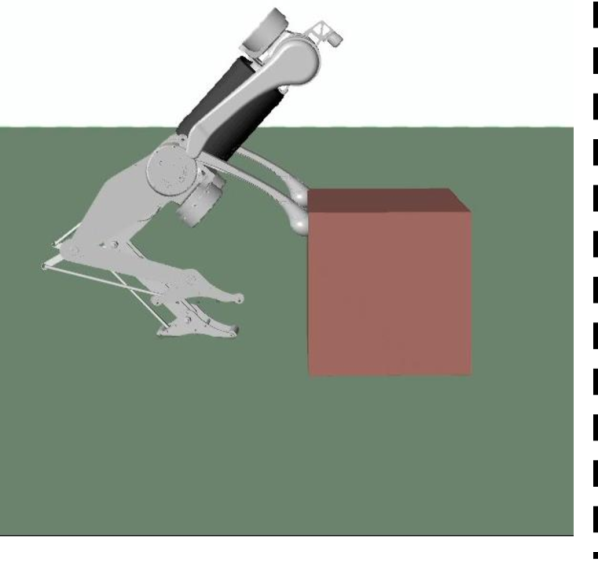
(a) 5 kg, 0.3 m cube,
$\mu_{g}$ = 0.7

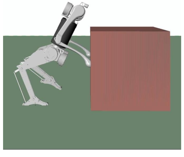
(b) 10 kg, 0.5 m cube,
 $\mu_{g}$ = 0.4

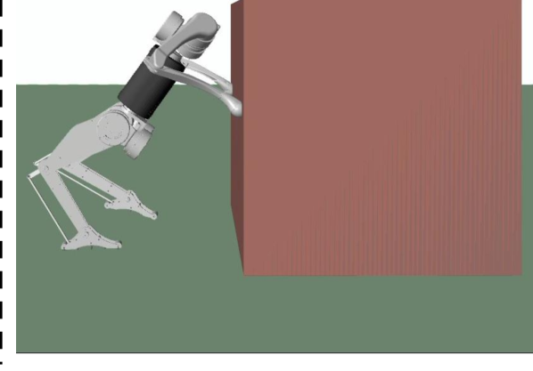
(c) 15 kg, 0.7 m cube,
$\mu_{g}$ = 0.5

Figure 1: Humanoid Robot Pushing Various Objects with Optimized Poses. Simulation video: https://youtu.be/iunrSQjQx4M

Trajectory optimization is a widely used motion planning technique [19, 13, 14]. It involves optimizing the robot’s body trajectory and foot positions over a specified time period and then tracking these optimal trajectories using real-time feedback control. In our approach, we propose kinodynamics-based pose optimization as a planner for generating optimal pushing poses. Our kinodynamics model incorporates simplified object-robot dynamics with robot kinematic constraints. Instead of optimizing the robot’s complete trajectory, pose optimization aims to find a single optimal pose for the entire pushing action, allowing for generalized pushing motions and reducing computational complexity. In a previous work [20], pose optimization was introduced as a kinematic-based planner for wheel-legged quadrupedal robots to overcome high obstacles using whole-body motion. However, that work relied solely on kinematics and did not account for ground friction and object mass, which are crucial factors in non-prehensile loco-manipulation. Moreover, the optimal pushing pose is task-oriented and specific to each object setup, rather than being generalizable. Hence, in this work, kinodynamics-based pose optimization is used to determine the most suitable optimal pose for each setup.

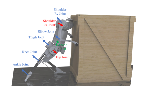
Figure 2: Humanoid Robot Model and Joint Definitions (Pose in this render does not imply the resulting pose from the proposed approach)

In [21, 22], non-prehensile loco-manipulation on humanoid robots was studied, employing techniques like RRT for planning object, body, or footstep paths throughout the entire trajectory. In another study [23], whole-body poses were used to apply a specific amount of pushing force during humanoid pushing. The desired poses and contact locations were determined based on the desired force using a randomization-based algorithm, and impedance control was employed to realize the desired behavior on humanoid robots. In our approach, we utilize pose optimization to generate whole-body poses while considering object parameters. The optimal pushing pose is obtained by solving an NLP problem that incorporates object-robot kinodynamics constraints. Unlike previous methods, we focus solely on generating a single pushing pose for the entire task rather than solving for object or robot trajectories within the pose optimization process. Additionally, we combine pose optimization with an online loco-manipulation MPC to track the optimal pose and coordinate whole-body manipulation and locomotion. Our MPC framework also allows for real-time responses to external disturbances.

The main contributions of the paper are as follows:

• We developed a novel kinodynamic-based pose optimization framework to solve for optimal pushing poses on humanoid robots with the consideration of object-robot steady-state dynamics, kinematics, and physical properties.

• Pose optimization generates unique poses that correspond to different setups, such as object size, object mass, and friction coefficients. The NLP problem can be efficiently solved with an average solving time of 250 ${\rm ms}$.

• We proposed a loco-manipulation MPC with a unified object-robot dynamics model, which optimizes pushing and ground reaction forces for coordinated whole-body loco-manipulation while tracking the optimal pose.

• The proposed framework can allow successful loco-manipulation control with a wide range of object parameter setups, including object side length in the range of 0.3 ${\rm m}$ to 1 ${\rm m}$, and object mass up to 20 ${\rm kg}$.

• The proposed control framework can recover deviations from desired states after introducing a 120 ${\rm N}$ lateral force for 0.3 ${\rm s}$ to the object,

The rest of the paper is organized as follows. Section. II presents the overview of the control system architecture. Section.III introduces the details of the robot model, unified robot-object dynamics, pose optimization framework, and the loco-manipulation MPC. Some simulation result highlights and comparisons are presented in Section. IV.

II System Overview

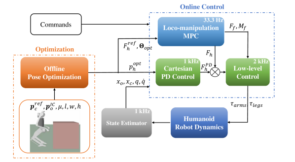
Figure 3: System Architecture

In this section, we introduce the control system architecture of the proposed approaches, depicted in Figure. 3. Firstly, using the kinodynamics-based pose optimization, we generate an optimal pushing pose considering the object’s initial states and physical properties, including dimension, mass, and friction coefficients. The kinodynamics model enables pose optimization to produce different poses for various object parameter setups, ensuring a large stability region and optimal hand contact locations for effective pushing action. Then, the obtained optimal pose and pushing reaction forces serve as references for the loco-manipulation MPC. The MPC leverages the unified dynamics of the object-robot system to coordinate the manipulation and locomotion tasks, incorporating whole-body pushing motion.

The kinodynamics-based pose optimization serves as a planner for solving the humanoid pushing pose. The information used in pose optimization includes the object’s initial CoM position $\bm{p}_{o}^{IC}\in\mathbb{R}^{3}$, the robot reference CoM position when initializing the pushing task $\bm{p}_{c}^{ref}\in\mathbb{R}^{3}$, friction coefficients at different contact locations, and object dimensions, where $l,w,$ and $h$ are the length, and width, and height of the rectangular object. The optimal pushing pose is solved in terms of optimal body Euler angles $\bm{\Theta}^{opt}$ and robot joint angles $\bm{q}\in\mathbb{R}^{16}$. Pose optimization also generates a reference pushing reaction force for MPC $\bm{F}_{h}^{ref}\in\mathbb{R}^{3}$.

The loco-manipulation MPC serves as an online feedback controller to control the arms and stance leg for manipulating the object while performing stable locomotion. It tracks the optimal Euler angles and optimizes pushing reaction forces $\bm{F}_{h,n}\in\mathbb{R}^{3}$ and ground reaction forces and moments $\bm{F}_{f,m}\in\mathbb{R}^{3},\bm{M}_{f,m}\in\mathbb{R}^{2}$.

A Cartesian PD controller is used in parallel with MPC for controlling the swing leg and hand locations. To compute arm and leg joint torques commands $\bm{\tau}_{arm,n}\in\mathbb{R}^{3},\>\bm{\tau}_{leg,m}\in\mathbb{R}^{5}$, in low-level control, we use whole-body contact Jacobians $\bm{J}_{c}$ to map forces and moments to joint torques.

There are several state feedback information we acquire from the robot. The robot state feedback $\bm{x}_{c}$ include body Euler angles (roll, pitch, and yaw) ${\bm{\Theta}_{c}=[\phi_{c},\>\theta_{c},\>\psi_{c}]}^{\intercal}$, CoM location $\prescript{}{\mathcal{}}{\bm{p}_{c}}\in\mathbb{R}^{3}$, velocity of body CoM $\prescript{}{\mathcal{}}{\dot{\bm{p}}_{c}}\in\mathbb{R}^{3}$, and angular velocity $\bm{\omega}_{c}\in\mathbb{R}^{3}$. The object state feedback $\bm{x}_{o}$ include object Euler angles ${\bm{\Theta}_{o}=[\phi_{o},\>\theta_{o},\>\psi_{o}]}^{\intercal}$, object CoM location $\prescript{}{\mathcal{}}{\bm{p}_{o}}\in\mathbb{R}^{3}$, velocity of object CoM $\prescript{}{\mathcal{}}{\dot{\bm{p}}_{o}}\in\mathbb{R}^{3}$, and angular velocity $\bm{\omega}_{o}\in\mathbb{R}^{3}$. Joint feedback includes the joint positions $\bm{q}$ and velocities $\dot{\bm{q}}$ of the humanoid robot.

III Proposed Approach

In this section, we introduce the proposed approach established in this work, including the details of dynamics models of the loco-manipulation system, kinodynamics-based pose optimization, and loco-manipulation MPC.

III-A Robot Dynamics Models

The humanoid robot design, shown in Figure 2, is followed from our previous work [16] and features a compact humanoid robot with 5-DoF legs and 3-DoF arms. The robot has an overall mass of 17 ${\rm kg}$. All joints are actuated by Unitree A1 torque-controlled motors with a maximum torque output of 33.5 ${\rm Nm}$ and maximum joint speed output of 21.0 ${\rm rad/s}$, except for the knee joints, which have a maximum torque output of 67 ${\rm Nm}$ due to halved gear ratio.

Firstly, we present the joint-space full dynamics equation of the humanoid robot. The joint-space generalized states ${\mathbf{q}}\in\mathbb{R}^{22}$ include $\bm{p}_{c},\mathbf{\Theta}_{c}$, and $\bm{q}$.

$${\color[rgb]{0,0,0}\mathbf{H}(\mathbf{q})\ddot{\mathbf{q}}+\mathbf{C}(\mathbf{q},\dot{\mathbf{q}})=\mathbf{\Gamma}+\bm{J}_{i}(\mathbf{q})^{\intercal}\bm{\lambda}_{i}}$$ (1)

where $\mathbf{H}\in\mathbb{R}^{22\times 22}$ is the mass-inertia matrix and $\mathbf{C}\in\mathbb{R}^{22}$ represents the joint-space bias force. $\mathbf{\Gamma}$ represents the actuation in the joint-space. $\bm{\lambda}_{i}$ and $\bm{J}_{i}$ represent the external force applied to the system and corresponding Jacobian matrix.

Next, we choose to simplify the dynamics of the humanoid robot when interacting with the object as the full dynamics equation (1) is highly complex and nonlinear. The dynamics model we developed is a simplified rigid-body dynamics (SRBD) model, shown in Figure. 4(b). We consider the robot trunk, shoulders, and hips as a combined rigid body and assume to ignore the dynamical effects of the lightweight and low-inertia arms and legs [10, 15]. The effects of ground reaction forces and external forces applied to the system can still be represented in this simplified model. The control inputs $\bm{u}=[\bm{u}_{h};\bm{u}_{f}]$ include pushing reaction forces $\bm{u}_{h}=[\bm{F}_{h,1};\>\bm{F}_{h,2}]$ at hands and ground reaction forces and moments $\bm{u}_{f}=[\bm{F}_{f,1};\>\bm{F}_{f,2};\>\bm{M}_{f,1};\>\bm{M}_{f,2}]$ at the foot locations, which are applied to the float base dynamics, where $\bm{F}_{h,n}=[F_{h,n,x};\>F_{h,n,y};\>F_{h,n,z}],\>\bm{F}_{f,m}=[F_{f,m,x};\>F_{f,m,y};\>F_{f,m,z}],$ and $\bm{M}_{f,m}=[M_{f,m,y};\>F_{f,m,z}]$. The 5-D ground reaction force control input is previously employed in [15] for bipedal locomotion.

Hence, the following equations of motion with respect to the robot CoM $\bm{p}_{c}$ are formed:

III-A1 Robot Dynamics

$$m_{b}(\ddot{\bm{p}}_{c}+\bm{g})=\mathbf{\Sigma}_{n=1}^{2}{\bm{F}_{h,n}}+\mathbf{\Sigma}_{m=1}^{2}{\bm{F}_{f,m}}$$ (2)

$$\prescript{}{\mathcal{G}}{\bm{I}_{c}}\bm{\dot{}}{\bm{\omega}}_{c}=\mathbf{\Sigma}_{n=1}^{2}({\bm{r}_{h,n}^{c}\times\bm{F}_{h,n}})+\mathbf{\Sigma}_{m=1}^{2}({\bm{r}_{f,m}^{c}\times\bm{F}_{f,m}})\\ +\mathbf{\Sigma}_{m=1}^{2}({\mathbf{L}\bm{M}_{f,m}})$$ (3)

In equation (2), $m_{b}$ denotes the robot mass and $\bm{g}=[0;\>0;\>-g]$ is the gravity vector. In equation (3), $\prescript{}{\mathcal{G}}{\bm{I}_{c}}$ is the robot body moment of inertia in the world frame, $\bm{r}_{h,n}^{c}\in\mathbb{R}^{3}$ is the position vector from robot CoM location to $n^{th}$ hand location $\bm{p}_{h,n}$ in the world frame, $\bm{r}_{f,m}^{c}\in\mathbb{R}^{3}$ is the position vector from robot CoM location to $m^{th}$ foot location $\bm{p}_{f,m}$ in the world frame, and $\mathbf{L}=[0,0;1,0;0,1]$ denotes the moment selection matrix to enforce 2-D moment control input [15].

The object dynamics is also a rigid body dynamics of the object, shown in Figure. 4(a). The robot pushing forces, $-\bm{u}_{h}$, normal force, $\bm{N}$, and simplified single-point friction force, $\bm{f}_{o}\in\mathbb{R}^{3}$, are applied to the object,

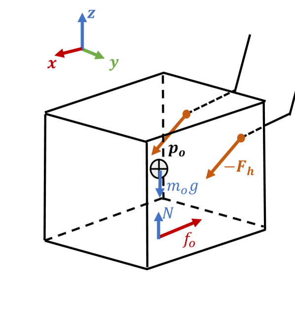
(a) Object Dynamics Model

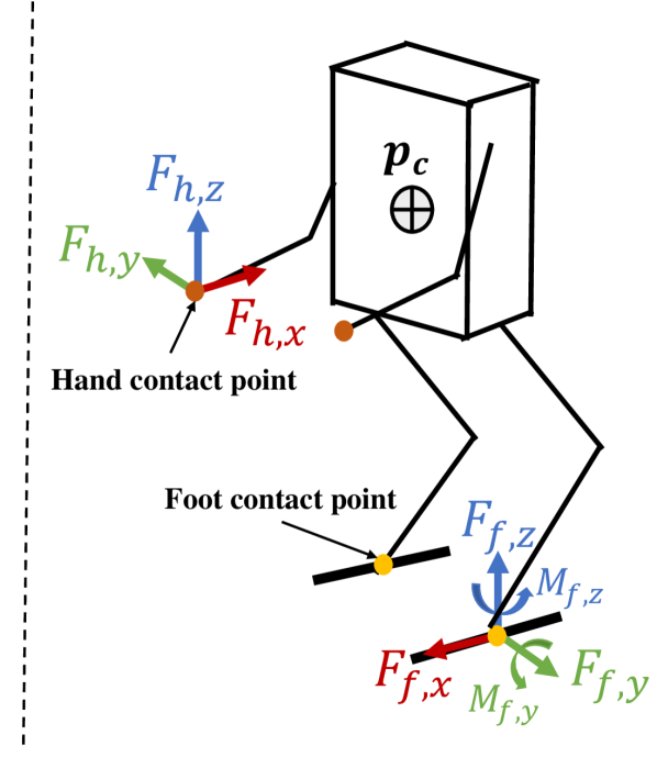
(b) Humanoid Dynamics Model

Figure 4: Dynamics Model Illustrations. a) Object under pushing, b) Humanoid SRBD

III-A2 Object Dynamics

$$m_{o}(\ddot{\bm{p}}_{o}+\bm{g})=-\mathbf{\Sigma}_{n=1}^{2}{\bm{F}_{h,n}}-\bm{R}_{o,z}\bm{f}_{o}+\bm{N}$$ (4)

$$\prescript{}{\mathcal{G}}{\bm{I}_{o}}\bm{\dot{}}{\bm{\omega}}_{o}=\mathbf{\Sigma}_{n=1}^{2}(\bm{r}_{h,n}^{o}\times-\bm{F}_{h,n})-\bm{R}_{o,z}\frac{h\bm{f}_{o}}{2}$$ (5)

In equation (4), $m_{o}$ denotes the object mass, $\bm{N}\in\mathbb{R}^{3}$ stands for the normal force supporting the object. It is assumed that the friction force is approximated by single contact friction at the projection of the object’s CoM on the ground and is always along the x-direction in the object frame during pushing, $\bm{f}_{o}=[\mu_{g}m_{o}g;0;0]$. $\mu_{g}$ is the coefficient of friction between the object and the ground and $\bm{R}_{o,z}$ is the 3-D rotation matrix defining the object’s yaw angle (i.e., assuming object pitch and roll are zero during pushing). In equation (5), $\prescript{}{\mathcal{G}}{\bm{I}_{o}}$ is the moment of inertia of the object estimated in the world frame, $\bm{r}_{h,n}^{o}\in\mathbb{R}^{3}$ stands for the position vector from object CoM location to $n^{th}$ hand location, and $h$ stands for the object height.

For pushing on flat ground, the object is assumed to have negligible z-direction acceleration.

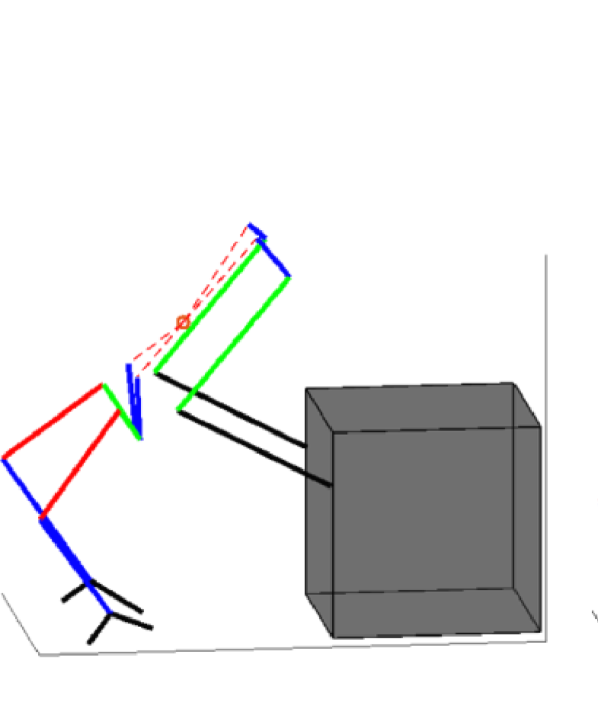
(a) 5 kg, 0.3 m cube,
$\mu_{g}$ = 0.7

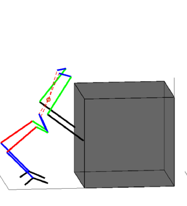
(b) 10 kg, 0.5 m cube,
$\mu_{g}$ = 0.4

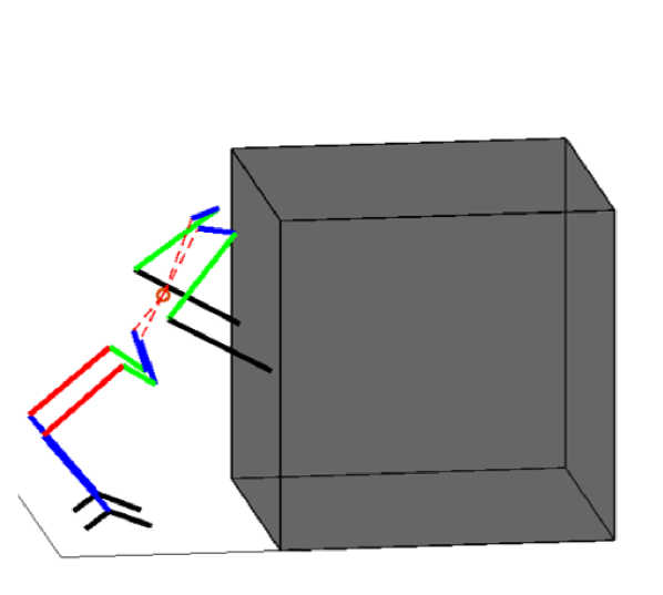
(c) 15 kg, 0.7 m cube,
$\mu_{g}$ = 0.5

Figure 5: Optimal humanoid Pushing Poses Solutions from Pose Optimization.

III-B Kinodynamics-based Pose Optimization

In this section, we will present the details of the kinodynamics-based pose optimization.

The utilization of whole-body flexibility and pose for pushing tasks is inspired by human observations. Humans lean their bodies forward, lower their center of mass, and position their feet further back to generate more force against object friction when pushing large and heavy objects. In the standard pushing pose for humanoid robots (i.e., nominal standing configuration), the feet align vertically with the center of mass. However, this configuration can negatively impact balancing and locomotion performance due to the generated moment from reaction forces during pushing, particularly with heavy objects. By shifting the center of mass forward and placing the feet further back, the gravitational force from the robot body and the ground reaction forces counteract the moment, providing more stable loco-manipulation.

In our approach, we employ a kinodynamics model in pose optimization. This model considers the simplified steady-state dynamics ((2-5)) of the object-robot system and applies kinematic constraints. Pose optimization differs from discretization-based trajectory optimization methods as it generates a single pose specific to the task at hand. To accommodate different gait types and ensure simplicity and flexibility, we focus on solving humanoid pushing poses with double-leg support. Furthermore, in pose optimization, we do not transmit ground reaction force and moment solutions to the MPC. This design choice allows for the generalization of the leg contact mode.

Another important feature of using the steady-state dynamics for the object model is its implication of preventing the robot from toppling over the box. The optimal pushing forces intend to prevent introducing a positive sum of moments in the y-direction with respect to the object CoM. Additionally, We choose to use the kinetic friction coefficients in equation (4-5) to optimize for more conservative reference pushing forces, as the static friction during the initial push is generally higher than kinetic friction. Thus the resulting more conservative pushing force will prevent introducing a large moment to top over the box during the initial push.

The pose optimization problem can be represented and solved as a NLP problem. The NLP problem’s optimization variable $\mathbf{X}$ contains robot CoM location $\bm{p}_{c}$, body Euler angles $\bm{\Theta}$, joint positions $\bm{q}$, and control inputs $\bm{u}$ (i.e., pushing reaction forces $\bm{F}_{h,n}$, and ground reaction forces and moments $\bm{F}_{f,m},\bm{M}_{f,m}$). The formal problem is defined as,

$$\underset{\mathbf{X}}{\operatorname{min}}\>\>\alpha(p_{c,z}^{ref}-p_{c,z})^{2}+||\bm{\Theta}||^{2}_{\bm{\beta}}+||\bm{u}||^{2}_{\bm{\gamma}}$$ (6)

$$\operatorname{s.t.}\>\text{Steady-state Dynamics Equations (\ref{eq:robotDynamicsForce}-\ref{eq:objectDynamicsMoment}})$$ (7a)

$$\bm{q}_{min}\leq\bm{q}\leq\bm{q}_{max}\quad\quad\quad\>\>$$ (7b)

$$\text{ Shoulder Location: }p_{s,n,x}\leq p_{h,n,x}\quad\>\>\>$$ (7c)

Contact Friction Cone Constraints:

$$\sqrt{F_{h,n,y}^{2}+F_{h,n,z}^{2}}\leq\mu_{f}|F_{h,n,x}|\quad\quad\quad$$ (7d)

$$\sqrt{F_{f,m,x}^{2}+F_{f,m,y}^{2}}\leq\mu_{h}|F_{f,m,z}|\quad\quad\>\>$$ (7e)

Pushing Contact Location Constraints:

$$p_{h,n,x}=p_{o,x}-\frac{l}{2}\quad\quad\quad\quad\quad\quad\quad\quad\>\>$$ (7f)

$$p_{o,y}-\frac{w}{2}\leq p_{h,n,y}\leq p_{o,y}+\frac{w}{2}\quad\quad\quad$$ (7g)

$$0\leq p_{h,n,z}\leq p_{o,z}+\frac{h}{2}\quad\quad\quad\quad\quad\quad\>\>$$ (7h)

$$p_{f,m,x}\leq p_{hip,m,x}\quad\quad\quad\quad\quad\quad\quad\quad\quad$$ (7i)

$$p_{f,m,z}=0\quad\quad\quad\quad\quad\quad\quad\quad\quad\quad\quad\>$$ (7j)

In equation (6), the objectives are driving pose CoM height close to reference (i.e., standing height), minimizing body rotations, specifically for roll and yaw, and minimizing control inputs. These objectives are weighted by scalar $\alpha\in\mathbb{R}$ and diagonal matrices $\bm{\beta}\in\mathbb{R}^{3\times 3},\bm{\gamma}\in\mathbb{R}^{16\times 16}$. In equation (7), $n^{th}$ hand location $\bm{p}_{h,n}$, shoulder location $\bm{p}_{s,n}$, $m^{th}$ foot location $\bm{p}_{f,m}$, and hip location $\bm{p}_{hip,m}$ are derived by forward kinematics based on joint positions. Equation (7b) describes the constraint for joint angle limits. Equation (7c) guarantees the shoulder location in the robot frame x-direction is always behind the hand location to avoid shoulder collision with the object in the optimal pose. Equation (7) and (7e) ensures the contact friction constraints are satisfied. $\mu_{f}$ and $\mu_{h}$ are the dynamic friction coefficients at the foot and hand contact points. Equation (7f) to (7h) ensures the pushing contact locations are on the object surface facing the robot. Equation (7i) ensures the foot contact locations are behind the hip locations in x-direction $p_{hip,m,x}$ for an adequate stability region. Lastly, equation (7j) constrains the foot contact locations both on the ground, as assumed double-leg contact mode in pose optimization.

III-C Humanoid Loco-manipulation MPC

This section presents the details of the proposed humanoid loco-manipulation MPC.

We choose to develop a loco-manipulation MPC for the humanoid pushing problem because the locomotion MPC we introduced in [15] lacks the consideration of pushing reaction forces or any information from the object. With small and light objects, the locomotion MPC and manually-fixed hand location are capable of handling them as external disturbances. However, with heavy objects, the locomotion MPC cannot adapt or perform well due to the pushing reaction force being too large to be considered perturbations.

With the loco-manipulation MPC, we intend to allow the humanoid robot to coordinate the motions of the entire body in a unified framework. We use this MPC to control manipulation and locomotion altogether to achieve pushing large, heavy, and ungraspable objects. To do so, first, we inform the MPC of the object state and directly control the object as an MPC objective, secondly, the MPC is employed with the unified object-robot dynamics introduced in equation (2-5). In addition, it optimizes the pushing and ground reaction forces while tracking the optimal pose from pose optimization.

Now we present the state-space formulation of the proposed dynamics equations of the robot-object system in this MPC. We choose the state variables as a combination of robot states, object states, and gravity vector, $\bm{x}=[{\bm{\Theta}_{c}};{\bm{p}}_{c};{\bm{\omega}_{c}};\dot{{\bm{p}}}_{c};{\bm{\Theta}_{o}};{\bm{p}}_{o};{\bm{\omega}_{o}};\dot{{\bm{p}}}_{o};\bm{g}]\in\mathbb{R}^{27}$. The state-space equation then can be written in the form of $\bm{\dot{x}}=\bm{A}\bm{x}+\bm{B}\bm{u}$, where

$$\bm{A}=\begin{bmatrix}\bm{A}_{c}&\mathbf{0}_{12}&\vline\bm{A}_{c}^{g}\\ \mathbf{0}_{12}&\bm{A}_{o}&\vline\bm{A}_{o}^{g}\\ \hline\cr\mathbf{0}_{3\times 12}&\mathbf{0}_{3\times 12}&\vline\>\>\mathbf{0}_{3}\end{bmatrix}\ ,$$ (8)

$$\bm{A}_{c}=\left[\begin{array}[]{cccc}\mathbf{0}_{3}&\mathbf{0}_{3}&\mathbf{S}^{-1}(\bm{\Theta}_{c})&\mathbf{0}_{3}\\ \mathbf{0}_{3}&\mathbf{0}_{3}&\mathbf{0}_{3}&\mathbf{I}_{3}\\ \mathbf{0}_{3}&\mathbf{0}_{3}&\mathbf{0}_{3}&\mathbf{0}_{3}\\ \mathbf{0}_{3}&\mathbf{0}_{3}&\mathbf{0}_{3}&\mathbf{0}_{3}\end{array}\right],$$ (13)

$$\bm{A}_{o}=\left[\begin{array}[]{cccc}\mathbf{0}_{3}&\mathbf{0}_{3}&\mathbf{S}^{-1}(\bm{\Theta}_{o})&\mathbf{0}_{3}\\ \mathbf{0}_{3}&\mathbf{0}_{3}&\mathbf{0}_{3}&\mathbf{I}_{3}\\ \mathbf{0}_{3}&\mathbf{0}_{3}&\mathbf{0}_{3}&\mathbf{0}_{3}\\ \mathbf{0}_{3}&\mathbf{0}_{3}&\mathbf{0}_{3}&\mathbf{0}_{3}\end{array}\right],\>\mathbf{S}=\left[\begin{array}[]{ccc}{c_{\theta}}{c_{\psi}}&-{s_{\psi}}&0\\ {c_{\theta}}{s_{\psi}}&c_{\psi}&0\\ -s_{\theta}&0&1\end{array}\right]$$ (21)

$$\bm{A}_{c}^{g}=\left[\begin{array}[]{cccc}\mathbf{0}_{3},&\mathbf{0}_{3},&\mathbf{0}_{3},&\mathbf{I}_{3}\end{array}\right]^{\intercal},$$ (23)

$$\bm{A}_{o}^{g}=\left[\begin{array}[]{cccc}\mathbf{0}_{3},&\mathbf{0}_{3},&\left[\begin{array}[]{ccc}0&0&\frac{-\mu_{g}m_{o}h\bm{R}_{o,z}}{2\prescript{}{\mathcal{G}}{\bm{I}_{o}}}\\ 0&0&0\\ 0&0&0\end{array}\right],&\left[\begin{array}[]{ccc}0&0&{-\mu_{g}\bm{R}_{o,z}}\\ 0&0&0\\ 0&0&0\end{array}\right]\end{array}\right]^{\intercal}$$ (31)

$$\bm{B}=\left[\begin{array}[]{cccccc}\mathbf{0}_{3}&\mathbf{0}_{3}&\mathbf{0}_{3}&\mathbf{0}_{3}&\mathbf{0}_{3\times 2}&\mathbf{0}_{3\times 2}\\ \mathbf{0}_{3}&\mathbf{0}_{3}&\mathbf{0}_{3}&\mathbf{0}_{3}&\mathbf{0}_{3\times 2}&\mathbf{0}_{3\times 2}\\ \frac{\mathcal{S}(\bm{r}_{h,1}^{c})}{\prescript{}{\mathcal{G}}{\bm{I}_{c}}}&\frac{\mathcal{S}(\bm{r}_{h,2}^{c})}{\prescript{}{\mathcal{G}}{\bm{I}_{c}}}&\frac{\mathcal{S}(\bm{r}_{f,1}^{c})}{\prescript{}{\mathcal{G}}{\bm{I}_{c}}}&\frac{\mathcal{S}(\bm{r}_{f,2}^{c})}{\prescript{}{\mathcal{G}}{\bm{I}_{c}}}&\frac{\mathbf{L}}{\prescript{}{\mathcal{G}}{\bm{I}_{c}}}&\frac{\mathbf{L}}{\prescript{}{\mathcal{G}}{\bm{I}_{c}}}\\ \frac{\mathbf{I}_{3}}{m_{b}}&\frac{\mathbf{I}_{3}}{m_{b}}&\frac{\mathbf{I}_{3}}{m_{b}}&\frac{\mathbf{I}_{3}}{m_{b}}&\mathbf{0}_{3\times 2}&\mathbf{0}_{3\times 2}\\ \mathbf{0}_{3}&\mathbf{0}_{3}&\mathbf{0}_{3}&\mathbf{0}_{3}&\mathbf{0}_{3\times 2}&\mathbf{0}_{3\times 2}\\ \mathbf{0}_{3}&\mathbf{0}_{3}&\mathbf{0}_{3}&\mathbf{0}_{3}&\mathbf{0}_{3\times 2}&\mathbf{0}_{3\times 2}\\ -\frac{\mathcal{S}(\bm{r}_{h,1}^{o})}{\prescript{}{\mathcal{G}}{\bm{I}_{o}}}&-\frac{\mathcal{S}(\bm{r}_{h,2}^{o})}{\prescript{}{\mathcal{G}}{\bm{I}_{o}}}&\mathbf{0}_{3}&\mathbf{0}_{3}&\mathbf{0}_{3\times 2}&\mathbf{0}_{3\times 2}\\ -\frac{\mathbf{D}}{m_{b}}&-\frac{\mathbf{D}}{m_{b}}&\mathbf{0}_{3}&\mathbf{0}_{3}&\mathbf{0}_{3\times 2}&\mathbf{0}_{3\times 2}\\ \end{array}\right]$$ (40)

In equation (13), matrix $\mathbf{S}$ denotes the mapping between the time derivative of Euler angles and body angular speed, $s$ denotes sine operator, and $c$ denotes cosine operator. Note that $\mathbf{S}$ is not invertible at $\theta_{c}=\pm 90^{\circ}$. We intend not to allow the robot to have a pitch angle of $\pm 90^{\circ}$ in any tasks. In equation (40), the operator $\mathcal{S}$ denotes the skew-symmetric matrix transformation of corresponding position vectors. $\mathbf{D}$ is a diagonal matrix containing $[1,1,0]$, which serves to ensure the z-direction acceleration of the object is zero.

To use this linear state-space dynamics equation in MPC, we discretize it at $i^{th}$ time step with step duration $dt$,

$$\bm{x}[i+1]=\bm{{A}}_{d}[i]\bm{x}[i]+\bm{{B}}_{d}[i]\bm{u}[i]$$ (41)

$${\bm{A}}_{d}=\mathbf{I}_{27}+{\bm{A}}dt,\quad{\bm{B}}_{d}={\bm{B}}dt$$ (42)

The formulation of the MPC problem with finite horizon $k$ is written as follows,

$$\underset{\bm{x,u}}{\operatorname{min}}\>\mathbf{\Sigma}_{i=0}^{k-1}\>\{\>||\bm{x}[i+1]-\bm{x}^{ref}[i+1])||^{2}_{\bm{Q}_{i}}+||\bm{u}_{f}||^{2}_{\bm{R}_{i}}\\ +\mathbf{\Sigma}_{n=1}^{2}||\bm{F}_{h,n}[i]-\bm{F}_{h,n}^{ref}[i]||^{2}_{\bm{S}_{i}}\>\}$$ (43)

$$\>\>\operatorname{s.t.}\quad\bm{x}[i+1]=\bm{{A}}_{d}[i]\bm{x}[i]+\bm{{B}}_{d}[i]\bm{u}[i]\quad\quad$$ (44a)

$$-\mu_{f}^{\prime}{F}_{f,m,z}\leq F_{f,m,x}\leq\mu_{f}^{\prime}{F}_{f,m,z}\quad$$

$$-\mu_{f}^{\prime}{F}_{f,m,z}\leq F_{f,m,y}\leq\mu_{f}^{\prime}{F}_{f,m,z}\quad$$

$$-\mu_{h}^{\prime}{F}_{h,n,x}\leq F_{h,n,y}\leq\mu_{h}^{\prime}{F}_{h,n,x}\quad$$

$$-\mu_{h}^{\prime}{F}_{h,n,x}\leq F_{h,n,z}\leq\mu_{h}^{\prime}{F}_{h,n,x}\quad$$ (44b)

$$0<{F}_{h,min}\leq F_{h,n,x}\leq{F}_{h,max}\quad\>$$

$$0<{F}_{f,min}\leq F_{f,m,z}\leq{F}_{f,max}\quad\>$$ (44c)

$$\bm{\tau}_{min}\leq\bm{J}_{c}^{\intercal}\bm{u}\leq\bm{\tau}_{max}\quad\quad\quad\quad\quad\>\>$$ (44d)

$$\prescript{}{\mathcal{B}}{F_{h,n,y}}=0\quad\quad\quad\quad\quad\quad\quad\quad\quad\>$$ (44e)

$$\text{for swing leg:}\>\>\bm{u}_{f,m}=\mathbf{0}\quad\quad\quad\quad$$ (44f)

The objectives of the MPC problem are described in equation (43), which are tracking a reference trajectory based on the command, minimizing the ground reaction forces for efficient locomotion, and minimizing the deviation of optimized hand force compared to reference hand force from pose optimization. These objectives are weighted by diagonal matrices $\bm{Q}_{i}\in\mathbb{R}^{27\times 27},\bm{R}_{i}\in\mathbb{R}^{10\times 10},\bm{S}_{i}\in\mathbb{R}^{3\times 3}$ .

Equation (44a) to (44f) are constraints of the MPC problem. Equation (44a) is the dynamics constraint. Equation (44b) describes the conservative inscribed friction pyramid constraint of pushing and ground reaction forces, where $\mu^{\prime}=\sqrt{2}\mu/2$. Equation (44c) ensures the pushing and ground reaction forces are within limits. In addition, equation (44d) constrains the joint torque limit of the robot by using the whole-body contact Jacobian $\bm{J}_{c}$. In equation (44e), we constrain the hand force in the y-direction in the local frame to be zero, in order to avoid hand slip on the object during pushing. Equation (44f) ensures the swing leg exerts zero ground reaction force and moment.

The translation of the proposed MPC problem into Quadratic Programming (QP) form to be efficiently solved can be found in related works (e.g., [10], [24]).

III-D Low-level Control

Since the proposed loco-manipulation MPC provides the optimal pushing reaction forces for pushing and ground reaction forces and moments for the stance leg, we choose to use Cartesian PD to control hand and swing foot locations.

The desired swing foot location $\bm{p}_{f,n}^{des}\in\mathbb{R}^{3}$ follows a heuristic foot placement policy introduced in [25] and takes consideration of desired CoM linear speed, $\dot{\bm{p}}_{c}^{des}$ [12]. In addition, we adapt the heuristic foot placement by offsetting the desired capture point based on the optimal pose foot location $\bm{p}_{f,m}^{opt}$ and hip location $\bm{p}_{c}^{opt}$ for ensuring the stability region during walking.

$$\bm{p}_{f,m}^{des}=\bm{p}_{c}+(\bm{p}_{f,m}^{opt}-\bm{p}_{c}^{opt})+\dot{\bm{p}}_{c}\frac{\Delta t}{2}+k(\dot{\bm{p}}_{c}-\dot{\bm{p}}_{c}^{des})$$ (45)

where $\Delta t$ is the gait period, and $k$ is a scaling factor for tracking desired linear velocity.

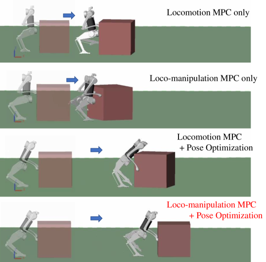
(a) Simulation snapshots.

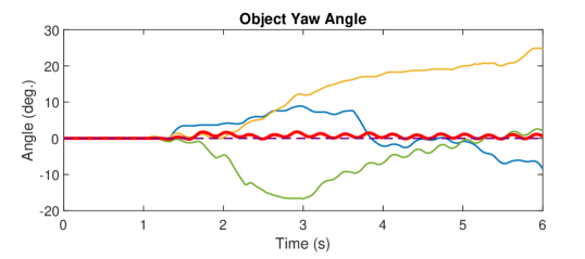
(b) Object Yaw Angle Comparison Plot.

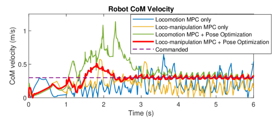
(c) Robot CoM Velocity Comparison Plot.

Figure 6: Comparison of Different Approaches in 2-D Object Pushing.

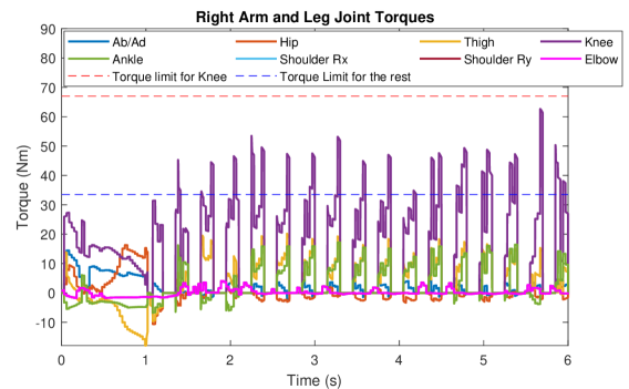
Figure 7: Right Arm and Leg Torque Plots in Simulation of Pushing 20 kg Object.

The Cartesian PD control law can then be applied to control $m^{th}$ swing foot to track the foot placement and $n^{th}$ hand to track optimal pushing contact location from pose optimization,

$$\bm{F}_{f,m}^{PD}=\bm{K}_{P}(\bm{p}_{f,m}^{des}-\bm{p}_{f,m})+\bm{K}_{D}(\dot{\bm{p}}_{f,m}^{des}-\dot{\bm{p}}_{f,m})$$ (46)

$$\bm{F}_{h,n}^{PD}=\bm{K}_{P}(\bm{p}_{h,n}^{opt}-\bm{p}_{h,n})+\bm{K}_{D}(\mathbf{0}-\dot{\bm{p}}_{h,n})$$ (47)

The aggregated PD forces $\bm{u}^{PD}$ is added to the optimized control inputs from MPC,

$$\bm{u}^{*}=\bm{u}+\bm{u}^{PD},$$ (48)

$$\bm{u}_{PD}=[\bm{F}_{h,1}^{PD};\>\bm{F}_{h,2}^{PD};\>\bm{F}_{f,1}^{PD};\>\bm{F}_{f,2}^{PD};\>\mathbf{0};\>\mathbf{0}]$$ (49)

The joint torque commands are approximated by mapping the total control input $\bm{u}^{*}$ with contact Jacobians,

$$\bm{\tau}=\bm{J}_{c}^{\intercal}\bm{u}^{*}.$$ (50)

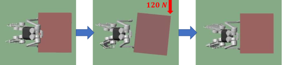
(a) Simulation Snapshots.

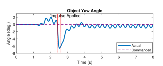
(b) Object Yaw Angle Plot.

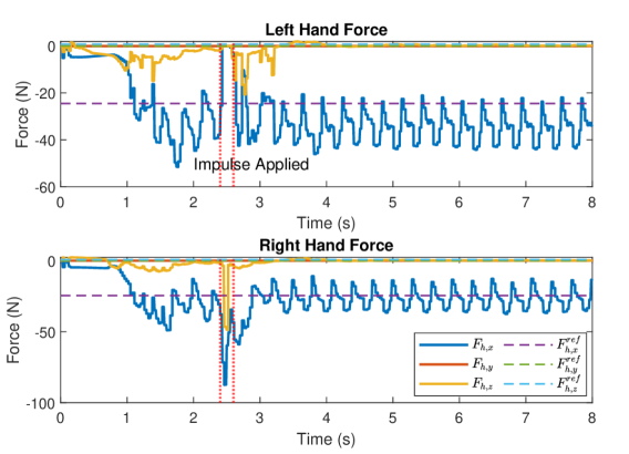
(c) Hand Reaction Force Plots.

Figure 8: Results of 2-D Pushing with External Impulse Perturbation.

IV Results

This section presents highlighted results of the proposed approaches in object-pushing tasks, including comparison with other approaches, pushing heavy objects, external force disturbance rejection, and tracking a desired object trajectory in 3-D. The reader is encouraged to watch the supplementary simulation videos for better visualization of the results.

To validate our proposed approaches, we set up a physical-realistic simulation framework in MATLAB Simulink with the Simscape Multibody library, which allows high-fidelity contact modeling in loco-manipulation simulations. We use CasADi [26] to solve pose optimization as an NLP problem with IPOPT solver. The average solving time for pose optimization with the proposed solver, out of 50 randomized setups, is 250 ${\rm ms}$. In this simulation, we assume the state information and physical properties of the object are known.

Weighting matrices in pose optimization and MPC are,

$$\bm{Q}_{i}=\text{diag}[1000,\>1000,\>500,\>500,\>500,\>500,\>10,\>10,\>5,\>1,\>1,\>1,\\ \>0,\>0,\>1000,\>500,\>500,\>0,\>0,\>0,\>10,\>1,\>1,\>0,\>0,\>0,\>1],\\ \bm{R}_{i}=\text{diag}[1,\>1,\>1,\>1,\>1,\>1,\>5,\>5,\>5,\>5]\times 10^{-4},\quad\quad\quad\>\\ \bm{S}_{i}=\text{diag}[1,\>1,\>1]\times 10^{-3}\quad\quad\quad\quad\quad\quad\quad\quad\quad\quad\quad\>\>\>\\ \alpha=50,\>\>\bm{\beta}=\text{diag}[50,\>5,\>50],\quad\quad\quad\quad\quad\quad\quad\quad\quad\quad\\ \bm{\gamma}=\text{diag}[1,\>1,\>1,\>1,\>1,\>1,\>1,\>1,\>1,\>1,\>1,\>1,\>5,\>5,\>5,\>5]\>$$ (51)

Note that the above parameters are universal to all simulation results.

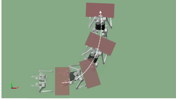
(a) Simulation Snapshots.

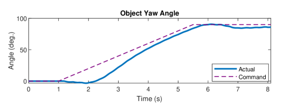
(b) Object Yaw Angle Plot.

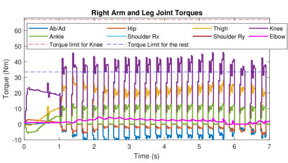
(c) Right Arm and Leg Joint Torque Plot.

Figure 9: Results of 3-D Pushing with 90-degree Turn.

IV-A Comparison of Approaches in 2-D Pushing

Firstly, we present a set of comparisons between different approaches in the humanoid robot 2-D pushing problem. The approaches we compared are

1. Locomotion MPC only;

2. Loco-manipulation MPC only;

3. Locomotion MPC and pose optimization;

4. Loco-manipulation MPC and pose optimization (proposed approach).

We compare these approaches by controlling the robot to push a 10 ${\rm kg}$ box on flat ground in the x-direction, with $\mu_{g}=0.5$. Figure. 6(a) shows the snapshots of the simulations. It is observed that the baseline locomotion MPC in [15] does not perform well since it does not optimize pushing force for loco-manipulation. The loco-manipulation MPC-only approach does not have an optimal hand location for pushing, resulting in ineffective corrections to the box yaw angle deviation. Combining the pose optimization and locomotion MPC, it is observed a better velocity tracking performance, as shown in Figure. 6(c). However, since hand forces and box states are not considered in the control framework, this approach struggles to keep the hands on the object during flight and failed due to the hand slipping out of the pushing surface. The proposed loco-manipulation MPC and pose optimization framework allow very stable pushing. With this proposed approach, it can be observed in Figure. 6(b) and 6(c), the box yaw angle stays around zero, and velocity follows the command.

IV-B Versatility of Pose Optimization

Pose optimization can generate different pushing poses for a range of object parameters. Object side lengths ($l,w,h$) range from 0.3 ${\rm m}$ to 1 ${\rm m}$. Object mass $m_{o}$ ranges from 1 ${\rm kg}$ to 20 ${\rm kg}$. Object-ground friction coefficient $\mu_{g}$ ranges from 0.2 to 0.7. Figure. 5 illustrates pushing poses generated by pose optimization based on varied object parameters, and Figure. 1 shows their corresponding simulation snapshots. Our proposed approach is capable of allowing our humanoid robot to push a very large and heavy object that has a side length of 1 ${\rm m}$ and mass of 20 ${\rm kg}$ (118$\%$ robot mass). The torque plot for pushing such objects in simulation with a desired velocity of 0.3 ${\rm m/s}$ is shown in Figure. 7. It can be observed that the motor torque limits are not exceeded during this task.

IV-C Robustness to External Disturbances

The proposed loco-manipulation MPC is capable of compensating for unknown external impulses applied to the system and recovering from such disturbances. Additionally, this MPC considers the object trajectory, enabling it to correct for perturbations to the object through the online controller. Simulation snapshots in Figure. 8(a) demonstrates the control framework’s ability to recover from an external impulse (120 ${\rm N}$ for 0.3 ${\rm s}$) applied to the object . In the object yaw angle plot in Figure. 8(b), it is shown that the proposed control framework reacts to the box yaw deviation quickly and effectively. In Figure. 8(c), it can be observed that the optimized pushing reaction forces from MPC stay close to the reference value from pose optimization during flight. During the application of external impulse, the controller has the knowledge of the deviation in object yaw angle, which results in zero reaction forces on the left hand and increased force magnitude on the right hand to correct this deviation.

IV-D 3-D Loco-manipulation

We have also extended our framework to 3-D which allows the robot to push an object given a specific trajectory or command to MPC. Figure. 9(a) shows the simulation snapshots of 3-D loco-manipulation with a 90-degree turn while pushing a 10 ${\rm kg}$ object with $\mu_{g}=0.4$. Figure. 9(b) presents the object yaw angle tracking with the proposed MPC. Lastly, Figure. 9(c) shows that the joint torque commands in the left arm and left leg are within limits.

V Conclusions

In conclusion, we propose a kinodynamics-based pose optimization and loco-manipulation MPC framework for humanoid robots to push heavy and large objects. The framework combines whole-body poses, coordinated locomotion and manipulation control. The offline pose optimization considers kinodynamics constraints to find an optimal pushing pose and reference forces. Then the online loco-manipulation MPC optimizes pushing and ground reaction forces for real-time control. Numerical simulations validate the framework’s effectiveness in pushing objects of different sizes and weights, handling external force perturbations, tracking state targets, and correcting state deviations.

References

- [1] S. Kuindersma, R. Deits, M. Fallon, A. Valenzuela, H. Dai, F. Permenter, T. Koolen, P. Marion, and R. Tedrake, “Optimization-based locomotion planning, estimation, and control design for the atlas humanoid robot,” Autonomous robots, vol. 40, pp. 429–455, 2016.
- [2] V. C. Paredes and A. Hereid, “Resolved motion control for 3d underactuated bipedal walking using linear inverted pendulum dynamics and neural adaptation,” in 2022 IEEE/RSJ International Conference on Intelligent Robots and Systems (IROS), pp. 6761–6767, IEEE, 2022.
- [3] https://www.youtube.com/watch?v=nRX6XvFUnls
- [4] D. Kim, S. J. Jorgensen, J. Lee, J. Ahn, J. Luo, and L. Sentis, “Dynamic locomotion for passive-ankle biped robots and humanoids using whole-body locomotion control,” The International Journal of Robotics Research, vol. 39, no. 8, pp. 936–956, 2020.
- [5] F. Abi-Farraj, B. Henze, C. Ott, P. R. Giordano, and M. A. Roa, “Torque-based balancing for a humanoid robot performing high-force interaction tasks,” IEEE Robotics and Automation Letters, vol. 4, no. 2, pp. 2023–2030, 2019.
- [6] C. D. Bellicoso, K. Krämer, M. Stäuble, D. Sako, F. Jenelten, M. Bjelonic, and M. Hutter, “Alma-articulated locomotion and manipulation for a torque-controllable robot,” in 2019 International conference on robotics and automation (ICRA), pp. 8477–8483, IEEE, 2019.
- [7] B. U. Rehman, M. Focchi, J. Lee, H. Dallali, D. G. Caldwell, and C. Semini, “Towards a multi-legged mobile manipulator,” in 2016 IEEE International Conference on Robotics and Automation (ICRA), pp. 3618–3624, IEEE, 2016.
- [8] X. Liu, Y. Zhao, D. Geng, S. Chen, X. Tan, and C. Cao, “Soft humanoid hands with large grasping force enabled by flexible hybrid pneumatic actuators,” Soft Robotics, vol. 8, no. 2, pp. 175–185, 2021.
- [9] C. Ott, O. Eiberger, W. Friedl, B. Bauml, U. Hillenbrand, C. Borst, A. Albu-Schaffer, B. Brunner, H. Hirschmuller, S. Kielhofer, et al., “A humanoid two-arm system for dexterous manipulation,” in 2006 6th IEEE-RAS international conference on humanoid robots, pp. 276–283, IEEE, 2006.
- [10] J. Di Carlo, P. M. Wensing, B. Katz, G. Bledt, and S. Kim, “Dynamic locomotion in the mit cheetah 3 through convex model-predictive control,” in 2018 IEEE/RSJ International Conference on Intelligent Robots and Systems (IROS), pp. 1–9, IEEE, 2018.
- [11] B. Katz, J. Di Carlo, and S. Kim, “Mini cheetah: A platform for pushing the limits of dynamic quadruped control,” in 2019 International Conference on Robotics and Automation (ICRA), pp. 6295–6301, IEEE, 2019.
- [12] D. Kim, J. Di Carlo, B. Katz, G. Bledt, and S. Kim, “Highly dynamic quadruped locomotion via whole-body impulse control and model predictive control,” arXiv preprint arXiv:1909.06586, 2019.
- [13] M. Chignoli, D. Kim, E. Stanger-Jones, and S. Kim, “The mit humanoid robot: Design, motion planning, and control for acrobatic behaviors,” in 2020 IEEE-RAS 20th International Conference on Humanoid Robots (Humanoids), pp. 1–8, IEEE, 2021.
- [14] J. Li and Q. Nguyen, “Dynamic walking of bipedal robots on uneven stepping stones via adaptive-frequency MPC,” IEEE Control Systems Letters, 2023.
- [15] J. Li and Q. Nguyen, “Force-and-moment-based model predictive control for achieving highly dynamic locomotion on bipedal robots,” in 2021 60th IEEE Conference on Decision and Control (CDC), pp. 1024–1030, IEEE, 2021.
- [16] J. Li and Q. Nguyen, “Multi-contact mpc for dynamic loco-manipulation on humanoid robots,” in 2023 American Control Conference (ACC), pp. 1215–1220, IEEE, 2023.
- [17] J.-P. Sleiman, F. Farshidian, M. V. Minniti, and M. Hutter, “A unified MPC framework for whole-body dynamic locomotion and manipulation,” IEEE Robotics and Automation Letters, vol. 6, no. 3, pp. 4688–4695, 2021.
- [18] A. Rigo, Y. Chen, S. K. Gupta, and Q. Nguyen, “Contact optimization for non-prehensile loco-manipulation via hierarchical model predictive control,” 2023 IEEE International Conference on Robotics and Automation (ICRA), 2023.
- [19] Q. Nguyen, M. J. Powell, B. Katz, J. Di Carlo, and S. Kim, “Optimized jumping on the mit cheetah 3 robot,” in 2019 International Conference on Robotics and Automation (ICRA), pp. 7448–7454, IEEE, 2019.
- [20] J. Li, J. Ma, and Q. Nguyen, “Balancing control and pose optimization for wheel-legged robots navigating high obstacles,” in 2022 IEEE/RSJ International Conference on Intelligent Robots and Systems (IROS), pp. 8835–8841, IEEE, 2022.
- [21] M. Murooka, I. Kumagai, M. Morisawa, F. Kanehiro, and A. Kheddar, “Humanoid loco-manipulation planning based on graph search and reachability maps,” IEEE Robotics and Automation Letters, vol. 6, no. 2, pp. 1840–1847, 2021.
- [22] P. Ferrari, M. Cognetti, and G. Oriolo, “Humanoid whole-body planning for loco-manipulation tasks,” in 2017 IEEE International Conference on Robotics and Automation (ICRA), pp. 4741–4746, IEEE, 2017.
- [23] M. Murooka, S. Nozawa, Y. Kakiuchi, K. Okada, and M. Inaba, “Whole-body pushing manipulation with contact posture planning of large and heavy object for humanoid robot,” in 2015 IEEE International Conference on Robotics and Automation (ICRA), pp. 5682–5689, IEEE, 2015.
- [24] J. L. Jerez, E. C. Kerrigan, and G. A. Constantinides, “A condensed and sparse QP formulation for predictive control,” in 2011 50th IEEE Conference on Decision and Control and European Control Conference, pp. 5217–5222, IEEE, 2011.
- [25] M. H. Raibert, Legged robots that balance. MIT press, 1986.
- [26] J. A. E. Andersson, J. Gillis, G. Horn, J. B. Rawlings, and M. Diehl, “CasADi – A software framework for nonlinear optimization and optimal control,” Mathematical Programming Computation, vol. 11, no. 1, pp. 1–36, 2019.