Effect of massive graviton on dark energy star structure
Abstract
The presence of massive gravitons in the field of massive gravity is considered an important factor in investigating the structure of compact objects. Hence, we are encouraged to study the dark energy star structure in the Vegh’s massive gravity. We consider that the equation of state governing the inner spacetime of the star is the extended Chaplygin gas, and then using this equation of state, we numerically solve the Tolman-Oppenheimer-Volkoff (TOV) equation in massive gravity. In the following, assuming different values of free parameters defined in massive gravity, we calculate the properties of dark energy stars such as radial pressure, transverse pressure, anisotropy parameter, and other characteristics. Then, after obtaining the maximum mass and its corresponding radius, we compute redshift and compactness. The obtained results show that for this model of dark energy star, the maximum mass and its corresponding radius depend on the massive gravity’s free parameters and anisotropy parameter. These results are consistent with the observational data and cover the lower mass gap. We also demonstrate that all energy conditions are satisfied for this model, and in the presence of anisotropy, the dark energy star is potentially unstable.
I Introduction
The existence of singularities in physics cannot be denied. Since a reliable physical theory must be free from these singularities, the existence of dark energy (DE) in various models (which include the cosmological constant , quintessence Caldwell1998 , phantom energy Caldwell2002 , Chaphygin gas Kamenshchik2001 , etc., which can provide an explanation for the accelerated expansion of the Universe) may be an option to resolve this problem in the case of compact objects. Several attempts were made to provide the models for compact objects and the existence of dark energy in them, including the introduction of false vacuum bubbles Coleman1980 , non-singular black holes Dymnikova1992 , gravastars MazurM2004 , and also dark energy stars (DES) ChaplinearXiv . The final stage of gravitational collapse of a compact object whose mass is greater than the mass of a neutron star, according to Chapline’s proposal ChaplinearXiv , turns into a DES in which there is no singularity in its center, and the surface of the star is introduced as a critical surface. In fact, for a compact object undergoing gravitational collapse, high-frequency quantum fluctuations exist near where the event horizon is defined. As a result of these very high-frequency fluctuations, it is expected that all nucleons in any kind of matter undergoing gravitational collapse will collectively decay into a mixture of leptons, photons, and vacuum energy droplets. This vacuum energy displays the difference in the ground state energy between a gas of quarks and a gas of leptons Chapline11 ; Barbieri1 ; Chapline2014 . However, these droplets of vacuum energy will be unstable because their mass is too small to satisfy the de Sitter condition a region of space with vacuum energy will be stable only if its radius is equal to its gravitational radius. Consequently, such droplets would immediately expand and coalesce, forming a uniform vacuum energy. Finally, after the escape of other decay products, only a compact object remains, whose inner region may be filled by vacuum energy Chapline11 ; Barbieri1 ; Chapline2014 .
After the introduction of DES, due to having very large vacuum energy in the center and the occurrence of phase transition on the surface, the presence of anisotropic pressure in it was investigated in several studies. Also, the non-establishment of the hydrostatic equilibrium regarding the isotropic pressure in gravastars Cattoen2005 , became another reason for the idea of anisotropy to remain strong in DES. A spherically symmetric model with a hypersurface was proposed by Lobo Lobo2006 , in which the negative radial pressure, positive anisotropy parameter, and negative gravity profile are the features of DES. For the first time, he investigated the stability of this star. Ghezzi Ghezzii2011 introduced a configuration of the inner spacetime of DES, which contained dark energy as well as a neutron gas. Unlike Lobo’s work Lobo2006 where the radial and transverse pressures were equal only at the center of the star, Ghezzi equated these two pressures inside the star and considered them to be different only at the surface. He showed that the maximum mass of DES depends on the coupling parameter. Also, a non-singular stable model of DES was presented in which the radial pressure was proportional to the matter density Rahaman2012 . On the other hand, a combination of baryonic matter and the phantom scalar field was a model that contained an exact solution for DES Yazadjiev2011 . In this way, various models of DES were presented over time, most of them referring to the anisotropy parameter and stability of the star. In addition, other definable properties were also studied for it BharR2015 ; Bharetal2018 ; Banerjee2020 ; Bhar2021 . Also, it was shown in Ref. Sakti2021 that the intervention of the phantom field can cause the instability of the star. The time dependence of Einstein’s equations and the existence of a negative final pressure for a DES created a configuration to have no central singularity BeltracchiG2019 . The radial oscillations of DES governed by the extended equation of state (EoS) of Chaplygin gas were measured by Panotopoulos et al. Panotopoulos2020 . Assuming the presence of slow rotations in DES, measurements for an isotropic sample showed that the moment of inertia of a rotating star is less than a non-rotating star Panotopoulos2021 . Solving the Einstein-Maxwell field equations in a model of Finch-Skea spacetime Finch was done by Malaver Malaver2022 . He stated that the physical parameters of a DES behave well in the presence of electric charge. Recently, for two cases of isotropic and anisotropic DESs, Pretel Pretel2023 investigated other physical quantities such as the radial pulsations and tidal deformation.
One approach in investigating the behavior of compact objects such as black holes and massive stars is to consider new gravitational fields, which can be followed in modified gravity. The black hole solution and their properties including thermodynamic properties, cosmic singularities, and entropy limit were studied in paradigmatic F(R) models Dombriz . Various studies were carried out, particularly on neutron stars in modified gravity. Yazadjiev et al. showed that the R-squared gravity parameter is effective in the neutron star mass-radius relations, however, it is comparable with other results obtained for the different equations of state Yazadjiev11 . By assuming slowly and rapidly rotating neutron stars in the R-squared gravity and gravity of modified gravity, it was argued that rotation increases the deviations from general relativity and the maximum mass and moment of inertia can reach higher values Staykov ; Yazadjiev12 . It was shown that in gravity in both the slowly and rapidly rotating modes, the relation can be distinguished from the results of general relativity (GR) compared to other modified gravity models, which can be used as an observational constraint in F(R) studies Doneva . In the context of gravity, it was also shown that the Tidal Love Numbers for non-rotating neutron stars can be several times larger compared to GR Yazadjiev13 . The interesting point is that in gravity, the maximum mass and compactness have smaller values compared to GR, which is similar to a repulsive field Feola . For other gravity models such as , it was indicated that the mass-radius relation strongly depends on the value of the curvature corrections, the sign of the correction parameters and the chosen equation of state Capozziello . In this regard, it was shown in a tensor scalar theory that for a rotating neutron star, the maximum mass can be greater than the maximum mass specified in GR Doneva1 . Another theory of modified gravity is of interests to models based on inflation. In response to the question that inflationary fields in various models such as the inflationary Higgs theory and attractor theories can be effective in the phenomenological description of the neutron star, Oikonomou showed that for the different equation of state models, the maximum mass obtained in these theories can increase compared to GR Oikonomou0 ; Oikonomou ; Oikonomou1 . To have a general and comprehensive view of other relativistic and non-relativistic stars structure in different theories of modified gravity, it is very useful to study reference Olmo .
Modified gravity can be important in the field of DES structure in two ways. First, in line with GR, it can improve the results of modified gravity compared to GR without changing the concept of dark energy. For example, Malaver et al. Malaver2021 showed that the physical properties of a DES are maintained in Einstein-Gauss-Bonnet gravity. Also, by assuming the dependence of metric potentials on energy, Tudeshki et al. Tudeshki2022 demonstrated in addition to satisfying the characteristics of DES, the stability of a star near the surface depends on energy, and the results obtained in gravity’s rainbow are improved compared to GR gravity. Secondly, the origin of the late acceleration of the Universe is not yet precisely known. In general, the concept of dark energy and the cosmological constant try to solve the problem based on the demand of GR.
However, persistent problems in cosmology have led to views of modified gravitation as an alternative to dark energy. One such theory is called massive gravity, which was first formulated by Pauli and Fierz PauliFierz . The introduction of a spin mass field in this theory, especially the assignment of mass to the graviton, became a turning point to justify the recent accelerated expansion at large distances without needing the dark energy. However, this linear theory had a fundamental flaw. In the massless limit of graviton, it does not satisfy GR. A non-linear method was an idea that Vainshtein Vainshtein offered to remove this problem. But Boulware and Deser (BD) BD showed that the existence of the ghost in this non-linear theory becomes another problematic factor. In order to solve this problem, there were many studies that have led to the formation of sub-branches in massive gravity. For example, the new massive gravity (NMG) in three dimensions Bergshoeff2009 . In 2009 and 2010 in two studies deRham2010 ; deRham2011 , it was shown that by using the graviton’s mass and polynomial interaction terms involved in spacetime action, BD-ghost can be prevented. This is possible by introducing a reference metric. This method is known as dRGT massive gravity. Providing an exact static solution of the black hole in this gravity Ghosh2016 allowed the study of compact objects in the presence of dRGT massive gravity to be strengthened. In particular, the presence of two additional terms in the massive metric coefficients compared to GR gravity can be a justification for dark matter and dark energy in massive gravity. It can be seen from this point of view that the massive graviton can play the role of the cosmological constant in cosmic distances Gumrukcuoglu ; Comelli ; Langlois ; Kobayashi . Also, the multi-gravity theory has tried to solve the BD-ghost problem in multi-dimensional spacetime for interacting spin- fields by applying the vielbein formulation Hinterbichler . In another interesting study, Hassan and Rosen showed that by using a dynamic reference metric instead of a static reference metric, the BD-ghost can be neglected in a non-linear bimetric theory for a massless spin- field Hassan and Rosen . A branch of dRGT massive gravity theory was proposed in 2013 by Vegh VegharXiv . By applying holographic principles and a singular reference metric, he was able to establish a ghost-free theory. After the introduction of Vegh’s model, many works were done in this field. Hendi et al., Hendi2016a ; Hendi2016b ; Hendi2016c ; Hendi2016d ; Hendi2016f ; Hendi2016g studied the stability and thermodynamics of black holes by investigating the effect of massive parameters. Also, in Ref. Hendi2017 , they investigated the physical quantities of the neutron star, including the maximum mass, using the AV18 potential method. Eslam Panah and Liu PanahLiu demonstrated that the maximum mass of a white dwarf in the presence of this gravity is greater than the Chandrasekhar limit. It was indicated that the end state of Hawking evaporation led to a black hole remnant in Vegh’s massive gravity, which could help to ameliorate the information paradox PanahHY . Also, there was a correspondence between black hole solutions of conformal and Vegh’s massive theories of gravity PanahH . The remarkable point in Vegh’s massive gravity is that the metric coefficients of spacetime do not have a term with the square of the distance . In the sense that cosmological constant can be defined for it separately. In addition, in the definition of a DES ChaplinearXiv , we are dealing with dark energy that has a much greater density than the cosmological constant. Therefore, in the present study, we investigate the physical characteristics of this compact object by using Vegh’s massive gravity and introducing dark energy in the form of fluid inside the inner spacetime.
In the last two decades, various observational and theoretical methods were introduced to constrain the range of graviton’s mass. Among others, we can mention the observation of gravitational waves emitted by the merger of a binary system, which was carried out by the LIGO-Virgo collaboration. In this measurement, the range of graviton’s mass in the GW170104 event was determined to be Scientific2018 . To learn about other methods, one can see Refs. Goldhaber ; Berti . On the other side of the theory, the idea is raised as to why should the mass of the graviton be constant. Attributing variable mass dependent on the scalar field is the work that was done in response to this question by Huang et al., Huang , which is known as mass-varying massive gravity (MVMG). Following that, a number of additional studies have been conducted, including investigating the effect of the massive graviton in strong and weak gravitational environments. The authors Zhang2018 suggested that the mass of graviton near a black hole could be orders of magnitude greater than that in the presence of weak gravitational fields. In this study, it was shown how, regardless of the presence of exotic matter or quantum effects, the mass of the graviton, which is approximately of Hubble scale in weak gravitational environments, can increase to approximately, near the event horizon of a black hole under environmental effects. Especially, it appears near the horizon and alters the GWs resulting from black hole mergers by producing ”echoes” at the end time Cardoso ; Cardoso1 . Also, in another study Sun , these effects on neutron stars and white dwarfs were checked, which showed that the results agreed with the Ref. Zhang2018 reported an increase in the mass of graviton near the star.
In the present work, in order to compare the behavior of DES in the presence of massive gravitons with the observational results obtained so far, we use the observational measurement of the GW190814 event Abbott2020 and the mass-radius relation for NS pulsars J1614-2230 Demorest2010 , J0348+0432 Antoniadis2013 , J0740+6620 Cromartie2020 and J2215+5135 Linares2018 . We also use the observational results of a binary system including the giant 2MASS J05215658+4359220 and a massive unseen companion Thompson2019 .
In this paper, we follow the scheme of this study as follows: in Sec. II, we take a look at the background and relations of Vegh’s massive gravity. Then, considering a spherically symmetric spacetime in Sec. III, we obtain the equations of motion and by using them, we introduce the TOV equation for the anisotropic distribution in Vegh’s massive gravity. In this section and in the following, we present EoS and a model for the existence of anisotropy. In Sec. IV, by numerically solving the modified TOV equation, we obtain and analyze the properties of DES, such as maximum mass and its corresponding radius, radial pressure and transverse pressure, anisotropy parameter, surface redshift, etc. Finally, in Sec. V, we present a summary of the results obtained from this study.
II Massive Gravity
In ghost free massive gravity, the action is given by deRham2011
| (1) |
where and are the speed of light and the gravitational constant, respectively. Also, is the Ricci scalar and refers to the graviton mass. In the second term on the right side of the action (potential term), are constant coefficients that play the role of free parameters of action. Also are introduced as symmetric polynomials of the eigenvalues of matrix . Here is dynamical metric tensor and is called the reference metric. At the end of the above action, implies the action of matter. are expressed in the following form
| (2) |
where , when . Note; in the above relations, the bracket marks indicate the traces in the form; and . Here we intend to specify the equations of motion in massive gravity, thus by varying the action with respect to metric tensor , and after doing some calculations, the equations are obtained as follows
| (3) |
where is Einstein tensor, is called massive tensor and is stress-energy tensor. Note; in the following, we use geometrized units for calculations. The massive tensor is extracted to form
| (4) |
where is related to the dimensions of spacetime. We work on 4-dimensional spacetime and so .
III Equations of motion and hydrostatic equilibrium equations
We consider a spherically symmetric spacetime with metric signature
| (5) |
where and are the metric potentials. The spatial reference metric or spatial fiducial metric is a suitable option for the black hole solutions VegharXiv ; Cai ; Hendi2017 ; PanahLiu . Hence we suppose
| (6) |
where is a positive constant. Using the line element Eq. (5) and reference metric Eq. (6), we can determine the tensor
| (7) |
and
| (12) | |||||
| (17) | |||||
| (22) |
and also
| (23) |
Since we are working on 4-dimensional spacetime, the only non-zero terms of are and Hendi2016g . Therefore, using Eqs. (2), (7) and (23), are obtained
| (24) |
By putting Eq. (24) in Eq. (4), the elements of the massive tensor are determined
| (25) |
We consider that the interior of the star is filled with an anisotropic fluid. The stress-energy tensor for an anisotropic distribution , is applied according to the following definition Bayin1986
| (26) |
where , , and are the energy density, the radial pressure, and the transverse pressure, respectively. Also refers to the four-velocity vector with , and represents the unit spacelike vector with . According to the metrics of the line element (5), the diagonal elements of the stress-energy tensor are obtained:
| (27) |
By substituting the above equations and the set of Eqs. (25) in Eq. (3), the equations of motion in massive gravity are obtained
| (28) | |||||
| (29) | |||||
| (30) |
where the prime and double prime are representing the first and second derivatives with respect to , respectively. By moving the graviton mass terms (the last term on the right side of the Eqs. (28) and (29)) to the other side of equality, one can see that the massive gravitons are similar to a fluid which has pressure and density. Another interesting point is that according to Eqs. (29) and (30), we realize that the pressure caused by gravitons is anisotropic. This anisotropic fluid can pattern the behavior of the dark matter halo on large scale Panpanich2018 .
The first equality of the equations of motion (28) leads us to the following relation
| (31) |
and
| (32) |
where shows the mass-energy function. Using the second equality (29), we obtain the gravity profile relation,
| (33) |
The conservation condition must be satisfied. So, we have . Now, by putting Eq. (33) in the conservation relation, and solving it in terms of the radial pressure gradient, the hydrostatic equilibrium equation in Vegh’s massive gravity for an anisotropic distribution is obtained in the following form,
| (34) |
In the next step, we must introduce the EoS that can show the behavior of dark energy, and a model to describe the fluid anisotropy in order to solve the modified TOV equation. A suitable choice is generalized Chaplygin gas EoS , plus a linear term, which is written as follows Debnath2004 ; Pourhassan2013 ,
| (35) |
where is a positive dimensionless constant, and is a positive dimension constant in units and the parameter is in the range . The first term is related to a barotropic fluid, and the second term refers to the generalized form of the Chaplygin gas EoS Bento2002 ; Gorini2003 ; Xu2012 . Such an EoS is an alternative to phantom and quintessence models in dark energy theory. We can consider the EoS (35) with in the following form for convenience in calculations, Tello2020 ; Panotopoulos2020 ; Panotopoulos2021
| (36) |
In this study, we have investigated the possibility of observing dark energy stars made of a fluid with a negative pressure and a barotropic component . The presence of barotropic term makes it possible to look at the system in such a way that it contains two fluids. It can be stated that in the presence of matter (regardless of its type and interactions), dark energy also exists inside the compressed body for some reasons. As a proposal, this model of dark energy stars may occupy somewhere between neutron stars and black holes. It is notable that, regardless of how the EoS of matter is defined, several studies have shown how the presence of dark energy affects the structure of other stars for example see Ref. Astashenok1 . In order to compare the results obtained from DES models with the extended Chaplygin EoS in GR Panotopoulos2020 ; Panotopoulos2021 and massive gravity (our suggestion), here we consider the constants and of the EoS as and . It should be noted that for the causality condition to be established at the star surface, the radial speed of sound must be satisfied in the range . Consequently, Pretel2023 . In this way, the permissible range for choosing constant values of is determined. By identifying the values of and keeping the considerations of density and numerical solution, can be selected.
The anisotropy parameter represents the difference between transverse pressure and radial pressure, . The main cause of anisotropy in compact objects is the presence of densities greater than the nuclear density, which can be due to the presence of condensation Hartle , phase transition Sokolov or electromagnetic fields Usov . It is important to determine which models can be proposed to correctly describe the anisotropy behavior (which is the difference between radial and transverse pressure inside the star). In this regard, several models for anisotropy have been proposed in various studies Bowers1974 ; Cosenza1981 ; Horvat2010 ; Doneva2012 ; Herrera2013 ; Raposo2019 . The model that we extract in the present work is a nonlinear anisotropy that was first proposed by Bowers and Liang Bowers1974 in general form and is expressed as follows,
| (37) |
where the constant measures the degree of anisotropy, and the constant is greater than . Since in a realistic model of compact objects , the allowed range is . In order to eliminate the anisotropy in the center of the star, we must consider . As a result, the final model of anisotropy parameter that we use in this study is defined as follows,
| (38) |
Therefore, our proposed model in this work for a dark energy star is introduced by extended Chaplygin gas Eq. (36) and the anisotropy parameter Eq. (38), which is formulated in the framework of massive gravity. For and , the results describe an isotropic DES in GR that depends only on the proposed model for the EoS Panotopoulos2020 ; Panotopoulos2021 .
IV Properties of dark energy stars in massive gravity
IV.1 Numerical Solutions
The star structure is determined by solving three coupled differential equations, Eqs. (32), (33), (34), and using the governing EoS (36) and anisotropy parameter (38). At the center of the star , the initial conditions are and , where is the central energy density. At the surface of the star, the radial pressure is negligible. Therefore, the boundary conditions on the surface are , and , where is the total mass of DES. After integration from the center to the surface of the star, the radius and mass are obtained. Also, due to the dependence of and to (or ), by considering different values of central energy density (or central radial pressure), we will be able to determine the maximum mass for DES models. In the numerical solution, it is important to pay attention to the fact that the anisotropy parameter is zero in the center (), and the energy density on the surface is . In addition, Eqs. (32) and (34) contain terms , , and constant that show the dependence of the solution on the mass of graviton and the free parameters. Here we consider the mass of graviton to be Ali2016 ; Hendi2017 ; PanahLiu . The results obtained from the numerical solution are presented for the central density , and the central pressure in Tables. 1-3.
| () | ||||
|---|---|---|---|---|
| (km) | ||||
|---|---|---|---|---|
| (km) | ||||
|---|---|---|---|---|
IV.2 Pressure, density and anisotropy
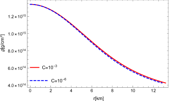
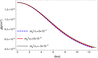
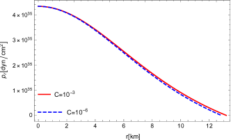
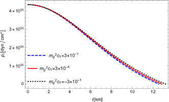
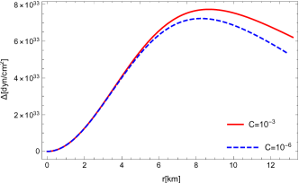
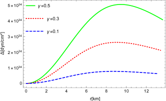
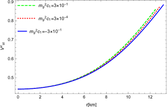
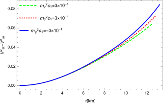
According to the Eqs. (32), (34), (35), (36) and (38), and by using a numerical solution, the density, radial pressure, and anisotropy parameter versus the radius are plotted in the Figs. 1-3, respectively. Figs. 1 and 2 show that the density and radial pressure are a decreasing function of the radius, as is expected. In both plots, it can be seen that the different values of , and affect the behavior of the density and radial pressure. It should be also noted that different values of have no effect on changes in these quantities. According to the left panel of Fig. 3, it can be seen that the anisotropy parameter is also sensitive to the parameter , and increases by its increasing. Therefore, the massive graviton and the dependence of its behavior on free parameters can affect the results obtained from density, pressure, and anisotropy. The factor creates a positive force in the outward direction of the star. This is an important feature of a DES, because it ensures the stability of the star.
It is interesting to examine the change in the behavior of the anisotropy parameter by changing the value of parameter versus radius. In the right panel of Fig. 3, the diagram is drawn in terms of different values of . It can be seen that by increasing , the amount of anisotropy also increases. This means that the force caused by it also increases towards the outside of the star, and the star will be more resistant to gravitational collapse.
IV.3 Maximum mass, compactness and surface redshift
Studying the structure of DESs in detail is difficult because the basic nature of dark energy is still unknown. Also, various models for the inner region of this star have been proposed so far. Depending on what the dark energy candidate is, and its other constituents, we will be able to estimate its mass function and maximum mass. In two studies Ghezzii2011 ; Bhar2021 , it was shown that the maximum mass of a DES is about and , respectively. For the special case of extended Chaplygin EoS, Panotopoulos et al. Panotopoulos2020 ; Panotopoulos2021 showed that these maxima depend on the constants of the EoS in the absence of anisotropy, and the maximum mass belongs to the category of heavy stars . Also, in a recent study Pretel2023 , it was shown that in the presence of anisotropy, and by assuming different values for constants of the EoS, the maximum mass can exceed the range of in GR. It is interesting to note that a similar result () was obtained for the maximum mass of the neutron star with the MPA1 EoS in the presence of inflationary attractor potentials compatible with the modified NICER constraints by Odintsov and Oikonomou Odintsov .
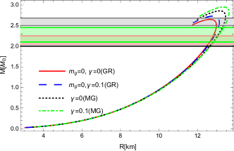
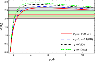
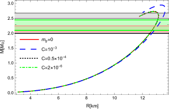
Fig. 4 demonstrates the mass-radius relation and central mass-density relation for different models (isotropic-anisotropic configuration in the framework of GR and isotropic and anisotropic configuration in the framework of massive gravity) of DES. The DES model we presented here evokes an isotropic (anisotropic) compact object in the GR with and or . For non-zero values of and or , a modified isotropic model (anisotropic model) of DES is created in massive gravity.
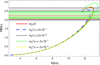
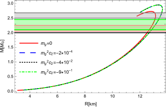
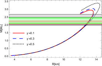
The gravitational mass versus radius diagrams in massive gravity (MG) for a series of central densities and for different values of , , and are drawn in Fig. 5. The maximum mass and radius of this model of DES increase with increasing , and reach the final limit for . On the other hand, as decreases, the maxima decrease and eventually reach the limit of the anisotropic model of GR (, and ) (see the up left panel in Fig. 5). For the positive values assigned to with a reduction of the order of , the maximum mass and radius have an increasing trend. But as the negative values of increase, the maxima are reduced (see the up right panel in Fig. 5). As it is clear from the results in the down left panel of Fig. 5, by considering different values of , the maximum mass and radius do not change, and remain fixed, but compared to the case (GR), an increasing in maximum mass and radius is observed. In fact, the obtained results depend on the choice of other massive free parameters. Also, we can see that as the anisotropy parameter increases, the maximum mass also increases in massive gravity (see the down right panel in Fig. 5). Note that according to Tables. 1-3 and Fig. 5, the maximum mass in massive gravity goes up to the interval , which can be located within the mass gap range, . This result, in addition to covering the observational constraints, can be a candidate for the massive unseen companion in the binary system 2MASS J05215658+4359220 whose mass range is estimated to be Thompson2019 , and remnant mass of GW190425 Abbott2020L ; Sedaghat2022 .
To calculate compactness , one needs to obtain the Schwarzschild radius in the massive gravity. The compactness can induce the power of gravity. By equalizing the Eq. (31) with zero, after some calculations, the modified Schwarzschild radius is determined as follows Hendi2017 ; PanahLiu ,
| (39) |
In general, the gravitational redshift is related to the metric potential, , which the surface redshift can be written in the following form using Eq. (31) in massive gravity Hendi2017 ,
| (40) |
For different values of , and , the obtained results are shown in Tables. 1-3. By changing the values of , the compactness and surface redshift do not change, and remain the same for all values (see Table. 3). The quantities and decrease by decreasing the values of (see Table. 2). By decreasing the positive and negative values assigned to , the quantities and increase slightly (refer Table. 1).
IV.4 ENERGY CONDITION
In order to have a standard stellar model, in addition to other acceptable properties, the energy conditions must be satisfied Leon1993 ; Visser1995 . For our proposed model for a DES discussed at the end of Sec. III, using the energy density , radial pressure and transverse pressure , we examine the energy conditions such as the null energy condition (NEC), weak energy condition (WEC), strong energy condition (SEC), and dominant energy condition (DEC) for DES. The requirements of each energy condition can be summarized as,
| (49) | |||||
| (56) |
Our results are given in Table. 4. As it is shown in Table. 4, the energy conditions are satisfied in inner DES. Although one of the characteristics of dark energy is the defect of the SEC condition (), however, the fluid behaves similarly to a normal matter in terms of energy conditions due to in the presence of barotropic fluid. It should be noted that the investigation of these conditions in the presence of gravitons with non-zero mass does not have different results from those in the case of gravitons with zero mass (GR).
| (NEC) | (WEC) | (SEC) | (DEC) |
| ✓ | ✓ | ✓ | ✓ |
IV.5 EQUILIBRIUM AND STABILITY
To check the stability of compact objects, several theoretical methods have been stated, which can be referred to as stability tests. Here we follow some cases.
IV.5.1 TOV equation
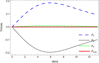
The structure of the star maintains its hydrostatic balance, if the sum of hydrostatic, gravitational, and anisotropic forces in the modified TOV equation becomes zero BharR2015 ; Bhar2021 . Therefore, the following relation must hold
| (57) |
where , , and , are the hydrostatic, gravitational and anisotropic forces, respectively. According to Eqs. (33), (34), and (38), the sum of forces can be obtained. Fig. 6 shows all forces and also their sum. It can be seen that the hydrostatic force and the anisotropy force are positive and act as repulsive forces against the gravitational force, which is negative and acts as an attraction force. Finally, these forces prevent the star from the gravitational collapse. Here, the second term of the EoS in the role of dark energy, as well as massive gravitons have anti-gravitational properties and lead to a resistance to the gravitational attraction. Therefore, the hydrostatic equilibrium is also established in massive gravity. It should be noted that in the structure of other compact objects such as neutron stars in the presence of modified gravity, anisotropy also creates a repulsive force that resists the gravitational collapse Nashed ; Nashed1 .
IV.5.2 Causality
The condition of causality holds if the speed of sound obeys the relation Herrera1992 . For an anisotropic configuration, two quantities, the square of the radial speed of sound and the square of the transverse speed of sound , can be measured as follows
| (58) | |||||
| (59) |
Here, the speed of sound is obtained numerically, and the results are plotted in Figs. 7 and 8. It can be clearly seen that for different values of massive free parameters, two conditions and are satisfied. Note that unlike what happens for the speed of sound inside the isotropic stars, here in the presence of an anisotropic configuration, the speed of sound can have an increasing trend.
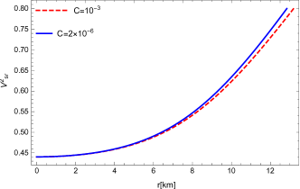
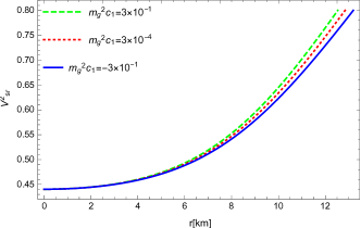
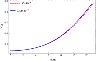
By reducing the massive parameter , the speed of sound decreases. Also, the lowest value of corresponds to negative values of . It is interesting to consider what consequences these local anisotropies can create in the star. Herrera Herrera1992 showed that in the presence of local anisotropies, a phenomenon called cracking occurs. Based on this idea, potentially stable regions and potentially unstable regions are distorted according to speeds Abreu2007 . According to Fig. 9, it is deduced that for non-zero values of , this anisotropic model Eq. (38) of DES is potentially unstable. This instability is caused by the presence of anisotropy in this configuration.
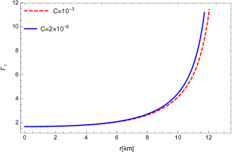
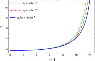
IV.5.3 Adiabatic index
The adiabatic index can determine the stiffness of EoS for a specific density. It is also a suitable quantity to check the stability of the star against the radial perturbations. According to some studies such as Chandrasekhar1964 ; Bondi1964 ; Chan1993 , a spherical configuration is stable if its adiabatic index be . The behavior of the adiabatic index is plotted in Fig. 10. It is clear that anywhere inside the DES, it has a value greater than . Therefore, it can be stated that the configuration of the star is dynamically stable in massive gravity with (isotropic), different values of and . But in the case of local anisotropy within the star, it was suggested to make corrections on the condition of adiabatic stability, although the relativistic corrections make the increasing for the instability Chan1992 ; Chan1993 . Therefore, we will try another method in the following.
IV.5.4 Harrison-Zeldovich-Novikov condition
Another example of the stability conditions of compact objects is known as Harrison-Zeldovich-Novikov condition Zeldovich1971 ; Harrison1965 , which states that there are stable regions where condition is valid. In the right panel of Fig. 4, the maximum mass diagram versus central density shows that the criterion is satisfied for the areas on the left side of the maximum point of the curves. So DES is stable up to this point with . As soon as we move from this density to higher densities (right side of the curves), becomes negative, which indicates dynamical instability, and the star becomes capable of collapsing into a black hole.
In general, it can be pointed out that the existence of instability in the structure of compact objects can be caused by the two factors of EoS and anisotropy. Of course, which model is better for these two factors is not completely clear because, for our chosen model, the main nature of dark energy is not yet known.
V Conclusions
In this paper, by considering the massive graviton, we obtained the hydrostatic equilibrium equation in Vegh’s massive gravity. For the extended Chaplygin gas EoS and a nonlinear model of anisotropy, the anisotropic modified TOV equation was solved numerically. After performing the numerical solution for the fixed coefficients of the EoS and , we obtained the density, radial pressure, and the anisotropy parameter depending on the mass of graviton . We also showed that with an increasing degree of anisotropy, the anisotropy parameter () increased. By increasing it up to a certain limit, the maximum mass and radius increase. The force created by the presence of anisotropy is a factor preventing gravitational collapse. We showed that the obtained results from the numerical solution were sensitive to the variation of the values of massive free parameters , and constant . We saw that by increasing , the maximum mass and radius are increased. Increasing the negative values of led to a decrease in the maximum mass and radius. It was also found that the change in values of has no effect on the maxima. We indicated that two important factors, the massive gravitons and anisotropy, can improve the obtained results compared with the mass-radius constraint from the observational events. We also demonstrated that in the isotropic model, massive gravitons alone have the ability to increase the maximum mass and radius. Our proposed model for DES not only might be a candidate for mystery object from the gravitational-wave signal of GW190814 Astashenok but also able to include mass values located in the lower mass gap range, Thompson2019 ; AbbottB.P . It was found that the compactness and the surface redshift of the DES did not change by variations , and by decreasing the value of , both decreased. Also, the highest value for the compactness and the surface redshift was related to the negative value of , and the lowest value was obtained for the positive value of . In order to investigate the stability of the DES structure, we used several different methods. We showed that the causality condition holds for the anisotropic configuration, but this model is potentially unstable. On the other hand, the star was dynamically stable for central densities lower than the critical density, and for densities higher than , it became unstable, and it was possible to become a black hole. In summary, DESs were important in the framework of massive gravity, because the role of massive gravitons in this method made the proposed model closer to the observational results. It would be interesting to use different methods applied for neutron star Bauswein ; Raaijmakers ; Altiparmak in future studies in order to constrain the mass and radius of the DES by observational data such as tidal deformability from the event GW170817, and other information.
Acknowledgements.
We would like to thank the referee for the good comments and advice that improved this paper. ABT and GHB wish to thank Shiraz University research council. BEP thanks the University of Mazandaran. The University of Mazandaran has supported the work of BEP by title ”Evolution of the masses of celestial compact objects in various gravity”.References
- (1) R. R. Caldwell, R. Dave, and P. J. Steinhardt, Phys. Rev. Lett. 80 (1998) 1582.
- (2) R. R. Caldwell, Phys. Lett. B 545 (2002) 23.
- (3) A. Kamenshchik, U. Moschella, and V. Pasquier, Phys. Lett. B 511 (2001) 265.
- (4) S. Coleman, and F. De Luccia, Phys. Rev. D 21 (1980) 3305.
- (5) I. Dymnikova, Gen. Rel. Grav. 24 (1992) 235.
- (6) P. O. Mazur, and E. Mottola, Proc. Nat. Acad. Sci. 101 (2004) 9545.
- (7) G. Chapline, ”Dark Energy Stars”, [arXiv:astro-ph/0503200], 2005.
- (8) G. Chapline, Int. J. Mod. Phys. A 18 (2003) 3587.
- (9) J. Barbieri, and G. Chapline, Phys. Lett. B 709 (2012) 114.
- (10) G. Chapline, and J. Barbieri, Int. J. Mod. Phys. D 23 (2014) 1450025.
- (11) C. Cattoen, T. Faber, and M. Visser, Class. Quantum Grav. 22 (2005) 4189.
- (12) F. S. Lobo, Class. Quantum Grav. 23 (2006) 1525.
- (13) C. R. Ghezzi, Astrophys. Space Sci. 333 (2011) 437.
- (14) F. Rahaman, R. Maulick, A. K. Yadav, S. Ray, and R. Sharma, Gen. Rel. Grav. 44 (2012) 107.
- (15) S. S. Yazadjiev, Phys. Rev. D 83 (2011) 127501.
- (16) P. Bhar, and F. Rahaman, Eur. Phys. J. C 75 (2015) 1.
- (17) P. Bhar, T. Manna, F. Rahaman, and A. Banerjee, Can. J. Phys. 96 (2018) 594.
- (18) A. Banerjee, M. Jasim, and A. Pradhan, Mod. Phys. Lett. A 35 (2020) 2050071.
- (19) P. Bhar, Phys. Dark Universe. 34 (2021) 100879.
- (20) M. F. A. Rangga Sakti, and A. Sulaksono, Phys. Rev. D 103 (2021) 084042.
- (21) P. Beltracchi, and P. Gondolo, Phys. Rev. D 99 (2019) 044037.
- (22) G. Panotopoulos, A. Rincon, and I. Lopes, Eur. Phys. J. Plus. 135 (2020) 1.
- (23) G. Panotopoulos, A. Rincon, and I. Lopes, Phys. Dark Universe. 34 (2021) 100885.
- (24) M. R. Finch, and J. E. Skea, Class. Quantum Grav. 6 (1989), 467.
- (25) M. Malaver, ”Charged Dark Energy Stars in a Finch-Skea Spacetime”, [arXiv:2206.13943], 2022.
- (26) J. M. Pretel, Eur. Phys. J. C 83 (2023) 26.
- (27) A. de la Cruz-Dombriz, and D. Saez-Gomez, Entropy 14 (2012) 1717.
- (28) S. S. Yazadjiev et al., J. Cosmol. Astropart. Phys. 06 (2014) 003.
- (29) K. V. Staykov et al., J. Cosmol. Astropart. Phys. 10 (2014) 006.
- (30) S. S. Yazadjievet, D. D. Doneva, and K. D. Kokkotas, Phys. Rev. D 91 (2015) 084018.
- (31) D. D. Doneva, S. S. Yazadjiev, and K. D. Kokkotas, Phys. Rev. D 92 (2015) 064015.
- (32) S. S. Yazadjiev, D. D. Doneva, and K. D. Kokkotas, Eur. Phys. J. C 78 (2018) 818.
- (33) P. Feola et al., Phys. Rev. D 101 (2020) 044037.
- (34) S. Capozziello et al., Phys. Rev. D 93 (2016) 023501.
- (35) D. D. Doneva et al, Phys. Rev. D 98 (2018) 104039.
- (36) V. K. Oikonomou, Class. Quantum Grav. 38 (2021) 175005.
- (37) V. K. Oikonomou, Symmetry. 14 (2022) 32.
- (38) V. K. Oikonomou, MNRAS 520 (2023) 2934.
- (39) G. J. Olmo, D. R. Garcia, and A. Wojnar, Phys. Rep. 876 (2020) 1.
- (40) M. Malaver, et al., ”A theoretical model of Dark Energy Stars in Einstein-Gauss-Bonnet Gravity”,[arXiv:2106.09520].
- (41) A. Bagheri Tudeshki, G. H. Bordbar, and B. Eslam Panah, Phys. Lett. B 835 (2022) 137523.
- (42) M. Fierz, and W. E. Pauli, Proc. Roy. Soc. Lond. A 173 (1939) 211.
- (43) A. I. Vainshtein, Phys. Lett. B 39 (1972) 393.
- (44) D. G. Boulware, and S. Deser, Phys. Rev. D 6 (1972) 3368.
- (45) E. A. Bergshoeff, O. Hohm, and P. K. Townsend, Phys. Rev. Lett. 102 (2009) 201301.
- (46) C. de Rham, and G. Gabadadze, Phys. Rev. D 82 (2010) 044020.
- (47) C. de Rham, G. Gabadadze, and A. J. Tolley, Phys. Rev. Lett. 106 (2011) 231101.
- (48) S. G. Ghosh, L. Tannukij, and P. Wongjun, Eur. Phys. J. C 76 (2016) 1.
- (49) A. De Felice, A. E. Gumrukcuoglu, C. Lin, and S. Mukohyama, Class. Quantum Grav. 30 (2013) 184004.
- (50) D. Comelli, M. Crisostomi, F. Nesti, and L. Pilo, J. High Energy Phys. 3 (2012) 1.
- (51) D. Langlois, and A. Naruko, Class. Quantum Grav. 29 (2012) 202001.
- (52) T. Kobayashi, M. Siino, M. Yamaguchi, and D. Yoshida, Phys. Rev. D 86 (2012) 061505.
- (53) K. Hinterbichler, and R. A. Rosen, J. High Energy Phys. 7 (2012) 1.
- (54) S. F. Hassan, and R. A. Rosen, J. High Energy Phys. 2 (2012) 1.
- (55) D. Vegh, ”Holography without translational symmetry”, [ arXiv:1301.0537], 2013.
- (56) S. H. Hendi, B. Eslam Panah, and S. Panahiyan, J. High Energy Phys. 11 (2015) 157.
- (57) S. H. Hendi, S. Panahiyan, and B. Eslam Panah, J. High Energy Phys. 01 (2016) 129.
- (58) S. H. Hendi, S. Panahiyan, B. Eslam Panah, and M. Momennia, Annalen der Physik. 528 (2016) 819.
- (59) S. H. Hendi, B. Eslam Panah, and S. Panahiyan, Class. Quantum Grav. 33 (2016) 235007.
- (60) S. H. Hendi, B. Eslam Panah, and S. Panahiyan, J. High Energy Phys. 05 (2016) 029.
- (61) S. H. Hendi, R. B. Mann, S. Panahiyan, and B. Eslam Panah, Phys. Rev. D 95 (2017) 021501(R).
- (62) S. H. Hendi, G. H. Bordbar, B. Eslam Panah, and S. Panahiyan, J. Cosm. Astropart. Phys. 07 (2017) 004.
- (63) B. Eslam Panah, and H. L. Liu, Phys. Rev. D 99 (2019) 104074.
- (64) B. Eslam Panah, S. H. Hendi, and Y. C. Ong, Phys. Dark Universe. 27 (2020) 100452.
- (65) B. Eslam Panah, and S. H. Hendi, Europhys. Lett. 125 (2019) 60006.
- (66) L. I. G. O. Scientific, V. Collaboration, and B. P. Abbott, Phys. Rev. Lett. 121 (2018) 129901.
- (67) A. S. Goldhaber, and M. M. Nieto, Rev. Mod. Phys. 82 (2010) 939.
- (68) E. Berti, J. Gair, and A. Sesana, Phys. Rev. D 84 (2011) 101501.
- (69) Q. G. Huang, Y. S. Piao, and S. Y. Zhou, Phys. Rev. D 86 (2012) 124014.
- (70) J. Zhang, and S. Y. Zhou, Phys. Rev. D 97 (2018) 081501.
- (71) V. Cardoso, E. Franzin, and P. Pani, Phys. Rev. Lett. 116 (2016) 171101.
- (72) V. Cardoso, S. Hopper, C. F. B. Macedo, C. Palen-zuela, and P. Pani, Phys. Rev. D 94 (2016) 084031.
- (73) X. Sun, and S. Y. Zhou, Phys. Rev. D 101 (2020) 044060.
- (74) R. Abbott et al., Astrophys. J. Lett. 896 (2020) L44.
- (75) P. Demorest, T. Pennucci, S. Ransom, M. Roberts, and J. Hessels, Nature. 467 (2010) 1081.
- (76) J. Antoniadis et al., Science 340 (2013) 1233232.
- (77) H. T. Cromartie et al., Nat. Astronomy. 4 (2019) 72.
- (78) M. Linares, T. Shahbaz, and J. Casares, Astrophys. J. 859 (2018) 54.
- (79) T. A. Thompson et al., Science 366 (2019) 637.
- (80) R. G. Cai, Y. P. Hu, Q. Y. Pan, and Y. L. Zhang, Phys. Rev. D 91 (2015) 024032.
- (81) S. S. Bayin, Astrophys. J. 303 (1986) 101.
- (82) S. Panpanich, and P. Burikham, Phys. Rev. D 98 (2018) 064008.
- (83) U. Debnath, A. Banerjee, and S. Chakraborty, Class. Quantum Grav. 21 (2004) 5609.
- (84) B. Pourhassan, Int. J. Mod. Phys. D 22 (2013) 1350061.
- (85) M. C. Bento, O. Bertolami, and A. A. Sen, Phys. Rev. D 66 (2002) 043507.
- (86) V. Gorini, A. Kamenshchik, and U. Moschella, Phys. Rev. D 67 (2003) 063509.
- (87) Y. D. Xu, Z. G. Huang, and X. H. Zhai, Astrophys. Space Sci. 339 (2012) 31.
- (88) F. Tello-Ortiz, M. Malaver, A. Rincon, and Y. Gomez-Leyton, Eur. Phys. J. C 80 (2020) 371.
- (89) A. V. Astashenok et al., Phys. Dark Universe. 42 (2023) 101295.
- (90) J. B. Hartle, R. F. Sawyer, and D. J. Scalapino, Astrophys. J. 199 (1975) 471.
- (91) A. I. Sokolov, J. Exp. Theor. Phys. 52 (1980) 575.
- (92) V. V. Usov, Phys. Rev. D 70 (2004) 067301.
- (93) R. L. Bowers, and E. P. T. Liang, Astrophys. J. 188 (1974) 657.
- (94) M. Cosenza, L. Herrera, M. Esculpi, and L. Witten, J. Math. Phys. 22 (1981) 118.
- (95) D. Horvat, S. Ilijic, and A. Marunovic, Class. Quantum Grav. 28 (2010) 025009.
- (96) D. D. Doneva, and S. S. Yazadjiev, Phys. Rev. D 85 (2012) 124023.
- (97) L. Herrera, and W. Barreto, Phys. Rev. D 88 (2013) 084022.
- (98) G. Raposo, P. Pani, M. Bezares, C. Palenzuela, and V. Cardoso, Phys. Rev. D 99 (2019) 104072.
- (99) A. F. Ali, and S. Das, Int. J. Mod. Phys. D 25 (2016) 1644001.
- (100) S. D. Odintsov, and V. K. Oikonomou, Phys. Rev. D 107 (2023) 104039.
- (101) B. P. Abbott, et al., Astrophys. J. Lett. 892 (2020) L3.
- (102) J. Sedaghat, et al., Phys. Lett. B 833 (2022) 137388.
- (103) J. Ponce de Leon, Gen. Rel. Grav. 25 (1993) 1123.
- (104) M. Visser, ”Lorentzian Wormholes. From Einstein to Hawking”. Woodbury, 1995.
- (105) G. G. L. Nashed, S. D. Odintsov, and V. K. Oikonomou, Eur. Phys. J. C 81 (2021) 528.
- (106) G. G. Nashed, S. D. Odintsov, and V. K. Oikonomou, Symmetry 14 (2022) 545.
- (107) L. Herrera, Phys. Lett. A 165 (1992) 206.
- (108) H. Abreu, H. Hernandez, and L. A. Nunez, Calss. Quantum. Grav. 24 (2007) 4631.
- (109) S. Chandrasekhar, Astrophys. J. 140 (1964) 417.
- (110) H. Bondi, Proc. R. Soc. Lond. A 281 (1964) 39.
- (111) R. Chan, L. Herrera, and N. O. Santos, Mon. Not. R. Astron. Soc. 265 (1993) 533.
- (112) R. Chan, L. Herrera, and N. O. Santos, Class. Quantum Grav. 9 (1992) 133.
- (113) Y. B. Zeldovich, and I. D. Novikov, Relativistic astrophysics. Vol.1: Stars and relativity, University of Chicago Press (1971).
- (114) B. K. Harrison, K. S. Thorne, M. Wakano, and J. A. Wheeler, Gravitation Theory and Gravitational Collapse, University of Chicago Press (1965).
- (115) In gravity, it was shown that the unknown component of the GW190814 event might be a neutron star, a rapidly rotating neutron star, or a black hole, [A. V. Astashenok, S. Capozziello, S. D. Odintsov, and V. K. Oikonomou, Phys. Lett. B 816 (2021) 136222].
- (116) B. P. Abbott et al., Astrophys. J. 882 (2020) L24.
- (117) A. Bauswein et al., Astrophys. J. Lett. 850 (2017) L34.
- (118) G. Raaijmakers et al., Astrophys. J. Lett. 918 (2021) L29.
- (119) S. Altiparmak, C. Ecker, and L. Rezzolla, Astrophys. J. Lett. 939 (2022) L34.