Certifiable Robustness for Naive Bayes Classifiers

Abstract.

Data cleaning is crucial but often laborious in most machine learning (ML) applications. However, task-agnostic data cleaning is sometimes unnecessary if certain inconsistencies in the dirty data will not affect the prediction of ML models to the test points. A test point is certifiably robust for an ML classifier if the prediction remains the same regardless of which (among exponentially many) cleaned dataset it is trained on.

In this paper, we study certifiable robustness for the Naive Bayes classifier (NBC) on dirty datasets with missing values. We present (i) a linear time algorithm in the number of entries in the dataset that decides whether a test point is certifiably robust for NBC, (ii) an algorithm that counts for each label, the number of cleaned datasets on which the NBC can be trained to predict that label, and (iii) an efficient optimal algorithm that poisons a clean dataset by inserting the minimum number of missing values such that a test point is not certifiably robust for NBC. We prove that (iv) poisoning a clean dataset such that multiple test points become certifiably non-robust is NP-hard for any dataset with at least three features. Our experiments demonstrate that our algorithms for the decision and data poisoning problems achieve up to $19.5\times$ and $3.06\times$ speed-up over the baseline algorithms across different real-world datasets.

PVLDB Reference Format:
PVLDB, 14(1): XXX-XXX, 2020.
doi:XX.XX/XXX.XX

PVLDB Artifact Availability:
The source code, data, and/or other artifacts have been made available at https://github.com/Waterpine/NClean.

1. Introduction

Machine Learning (ML) is becoming increasingly pervasive in modern society and is essential in critical decision-making processes. However, the success of most ML applications depends on obtaining high-quality training data. Unfortunately, in many real-world scenarios, the training data is often dirty for various reasons, such as noise introduced during the acquisition process, incomplete data, and human errors.

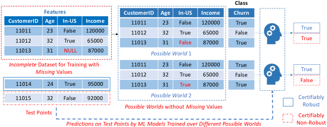
Figure 1. Example of an incomplete dataset, the possible worlds induced by the incomplete dataset, and the certifiably robust/non-robust predictions for data points with missing values over the possible worlds.

Data cleaning is the most commonly used approach to address these issues, with the goal of producing high-quality data. A long line of research has focused on developing powerful data cleaning tools (Peng et al., 2021; Rekatsinas et al., 2017a), using techniques from error detection (Abedjan et al., 2016; Mahdavi et al., 2019), missing value imputation (Trushkowsky et al., 2013), and data deduplication (Chu et al., 2016). Multiple data cleaning frameworks have been developed (Wang et al., 2014a; Krishnan et al., 2016; Krishnan et al., 2017). Data cleaning has also been studied under different contexts (Kohler and Link, 2021; Cheng et al., 2008; Bertossi et al., 2013; Khayyat et al., 2015; Bohannon et al., 2007; Prokoshyna et al., 2015). However, data cleaning is commonly seen as a laborious and time-intensive process in data analysis, albeit various efforts to accelerate the data cleaning process (Rekatsinas et al., 2017b; Chu et al., 2013; Chu et al., 2015a; Rezig et al., 2021). Furthermore, current data cleaning frameworks often are agnostic to the downstream applications, leading to extraneous costs spent on the cleaning process and causing unnecessary delays. For example, there has been a line of research focusing on cleaning only a subset of the dirty data to avoid the expensive cleaning costs (Wang et al., 2014b; Altowim et al., 2014). In light of this, a natural question to ask is whether we can minimize data cleaning by taking into account the downstream ML application.

Example 1.1.

Let’s take the example of a data analyst working at an insurance company trying to predict whether a customer will leave (churn) using an ML classifier. Figure 1 illustrates three customers with age, residency status (inside or outside the US), and income, which are features used for this classification task. The data for the customer with CustomerID 11013 is incomplete, as the residency information is missing (marked with NULL). Therefore there are two possible ways to clean the dataset: we can assign the missing feature “In-US” to either True or False, resulting in two possible worlds generated from the incomplete dataset.

For the customer with CustomerID 11014, the ML classifier may predict True for that customer in both possible worlds. If this information is known before training and making predictions, data cleaning can be skipped since the prediction is robust with respect to the missing value. However, the customer with CustomerID 11015 presents a different scenario, where the predictions made by the model trained on two possible worlds disagree: the ML classifier would predict True in the possible world where the feature “In-US” is False, but in the other possible world, the prediction is False. Therefore, data cleaning is necessary to predict the customer with CustomerID 11015 accurately.

To ensure that ML classifiers produce consistent predictions, we employ the notion certifiable robustness, which involves analyzing the possible worlds that can be generated from an incomplete or dirty dataset. A possible world (or cleaned dataset) of an incomplete (or dirty) dataset with missing values can be obtained by imputing each missing value (i.e., marked as NULL) with a valid value. In general, the prediction of an ML classifier may vary if it is trained on different cleaned datasets generated from a dirty dataset. However, these predictions may not be uniformly distributed among all possible labels and could potentially concentrate on a small subset of labels. Moreover, the predictions could remain the same regardless of which cleaned dataset is used. Formally, a test point is considered to be certifiably robust for an ML classifier when the classifier’s prediction for that test point remains the same regardless of which (among exponentially many) possible world generated from the incomplete dataset it was trained on, or certifiably non-robust otherwise. In Example 1.1, the customer with CustomerID 11014 is certifiably robust for the chosen ML classifier over the incomplete dataset, but the customer with CustomerID 11015 is certifiably non-robust. It is easy to see that if a test point is certifiably robust, then data cleaning is unnecessary because the ML model will give the same prediction when trained on any possible world.

To study the certifiable robustness of ML models on incomplete datasets, we consider the following problems:

Decision Problem: This involves determining whether a given test point is certifiably robust for a particular ML classifier, given an incomplete dataset.

Counting Problem: For each possible label, this problem involves counting the number of possible worlds on which the ML classifier can be trained to predict that label, given the incomplete dataset.

Data Poisoning Problem: This problem involves identifying the minimum number of cells in a clean dataset that need to be modified to NULL in order to make one or more test points certifiably non-robust for the ML classifier.

Efficient algorithms for the Decision Problem and Counting Problem can inform us of whether data cleaning is necessary and potentially allow for efficient model-specific data cleaning algorithms (Karlaš et al., 2020). Solving the Data Poisoning Problem can provide estimates on the safety of the training dataset from attacks and identify vulnerable datasets to poisoning, a task overlooked by prior work.

Although verifying whether a test point is certifiably robust is in general a computationally expensive task since it may require examing exponentially many possible worlds, it is possible to do so efficiently for some commonly used ML models. For example, recent research has demonstrated that it is possible to check whether a test point is certifiably robust for the $k$-Nearest Neighbor Classifier ($k$-NN) on datasets with missing values in polynomial time in the size of the dataset (Karlaš et al., 2020; Fan and Koutris, 2022). Thus, it is natural to consider whether it is possible to extend certifiable robustness to other machine learning models. In this paper, we provide a positive answer to this question by studying the certifiable robustness of the Naive Bayes Classifier (NBC), a widely-used model in fields such as the classification of RNA sequences in taxonomic studies (Wang et al., 2007), and spam filtering in e-mail clients (Sahami et al., 1998). Specifically, we focus on handling dirty datasets that contain missing values marked by NULL.

Contributions. In this paper, we study the three problems (i.e., Decision, Counting, and Data Poisoning) related to certifiable robustness for Naive Bayes Classifier (NBC), a simple but powerful supervised learning algorithm for predictive modeling that is widely used in academia and industry. Our main contributions are summarized as follows:

• We show that the Decision Problem for NBC can be solved in time $O(md+nd)$, where $n$ is the number of data points in the dataset, $m$ is the number of labels, and $d$ is the number of features. Since the training and classification for NBC also requires $O(md+nd)$ time, our algorithm exhibits no asymptotic overhead and provides a much stronger guarantee of the classification result compared to the original NBC;

• We present an algorithm for the Counting Problem for NBC that runs in time $O(dn^{md+1})$. While inefficient in practice, our algorithm does not explicitly enumerate every possible world of the incomplete dataset;

• We show that for a single test point, the Data Poisoning Problem for NBC can be solved in time $O(nmd)$; and for multiple test points, the Data Poisoning Problem is NP-hard for datasets containing at least three features; and

• We conduct extensive experiments using four real-world datasets and demonstrate that our algorithms exhibit up to $19.5\times$ speed-up over the baseline algorithms for the Decision Problem and $3.06\times$ speed-up for the Data Poisoning Problem.

Organization. The remainder of this paper is organized as follows. Section 2 introduces the notations used in this paper followed by necessary background and formal problem definition. We present the algorithms to solve the Decision Problem and Counting Problem for NBC in Section 3 and 4 respectively. In Section 5, we study the Data Poisoning Problem for single test point and multiple test points. Section 6 presents the experimental evaluation. We discuss the related work in Section 7 and conclude our paper in Section 8.

2. Preliminaries

Data Model. We assume a finite set of domain values for each attribute (or feature). For simplicity, we assume that every feature shares the same domain ${U}$, which contains a special element NULL. The set $\mathcal{X}={U}^{d}$ is a feature space of dimension $d$. A datapoint $\mathbf{x}$ is a vector in $\mathcal{X}$ and we denote $\mathbf{x}_{i}$ as the attribute value at the $i$-th position of $\mathbf{x}$. We assume a labeling function $\ell:\mathcal{X}\rightarrow\mathcal{Y}$ for a finite set of labels $\mathcal{Y}$. A training dataset $\mathcal{D}$ is a set of data points in $\mathcal{X}$, each associated with a label in $\mathcal{Y}$.

Missing Values and Possible Worlds. A data point $\mathbf{x}$ contains missing value if $\mathbf{x}_{i}=\texttt{NULL}$ for some $i$. A dataset $\mathcal{D}$ is complete if it does not contain data points with missing values, or is otherwise incomplete. We denote an incomplete dataset as $\mathcal{D}^{\square}$. For an incomplete dataset $\mathcal{D}^{\square}$, a possible world can be obtained by replacing each attribute value marked with NULL with a domain value that exists in $\mathcal{D}^{\square}$. This follows the so-called closed-world semantics of incomplete data. We denote $\mathcal{P}(\mathcal{D}^{\square})$ as the set of all possible worlds that can be generated from $\mathcal{D}^{\square}$. Given an ML classifier $f$, we denote $f_{\mathcal{D}}:\mathcal{X}\rightarrow\mathcal{Y}$ as the classifier trained on a complete dataset $\mathcal{D}$ that assigns for each complete datapoint $\bm{t}\in\mathcal{X}$, a label $f_{\mathcal{D}}(\bm{t})=l\in\mathcal{Y}$.

Certifiable Robustness. Given an incomplete dataset $\mathcal{D}^{\square}$ and an ML classifier $f$, a test point $\bm{t}$ is certifiably robust for $f$ over $\mathcal{D}^{\square}$ if there exists a label $l\in\mathcal{Y}$ such that $f_{\mathcal{D}}(\bm{t})=l$ for any possible world $\mathcal{D}\in\mathcal{P}(\mathcal{D}^{\square})$. Otherwise, the test point $\bm{t}$ is said to be certifiably non-robust.

Iif a test point $\bm{t}$ is certifiably robust, data cleaning on the incomplete dataset $\mathcal{D}^{\square}$ is unnecessary, since regardless of which possible world (or in other words, a clean dataset) we use as the training dataset, the prediction of $\bm{t}$ will remain the same. We remark that every test point is vacuously certifiably robust for any deterministic ML classifier over a complete dataset.

Naive Bayes Classifier. Naive Bayes Classifier (NBC) is a simple but widely-used ML algorithm. Given a complete dataset $\mathcal{D}$ and a complete datapoint $\bm{t}=(x_{1},x_{2},\dots,x_{d})$ to be classified, the datapoint is assigned to the label $l\in\mathcal{Y}$ such that the probability $\mathbb{P}[l\mid\bm{t}]$ is maximized. NBC assumes that all features of $\mathcal{X}$ are conditionally independent for each label $l\in\mathcal{Y}$ and estimates, by the Bayes’ Theorem, that

$$\mathbb{P}[l\mid\bm{t}] =\mathbb{P}[l]\cdot\mathbb{P}[\bm{t}]^{-1}\cdot\mathbb{P}[\bm{t}\mid l]$$

$$=\mathbb{P}[l]\cdot\mathbb{P}[\bm{t}]^{-1}\cdot\prod_{j=1}^{d}\mathbb{P}[x_{j}\mid l].$$

Finally, it assigns for each test point $\bm{t}=(x_{1},x_{2},\dots,x_{d})$, the label $l$ that maximizes $\mathbb{P}[l\mid\bm{t}]$.

To estimate the probabilities $\mathbb{P}[l]$ and $\mathbb{P}[x_{j}\mid l]$, NBC uses the corresponding relative frequency in the complete dataset $\mathcal{D}$, which we denote as $Pr(l)_{\mathcal{D}}$ and $Pr(x_{j}\mid l)_{\mathcal{D}}$ respectively. When a (complete or incomplete) dataset $\mathcal{D}$ of dimension $d$, a test point $\bm{t}=(x_{1},x_{2},\dots,x_{d})$ and $m$ labels $l_{1},l_{2},\dots,l_{m}$ are understood or clear from context, we denote $N_{i}$ as the number of data points in $\mathcal{D}$ with label $l_{i}$, $E_{i,j}$ as the number of existing data points $\mathbf{x}$ in $\mathcal{D}$ with label $l_{i}$ and has value $x_{j}$ as its $j$-th attribute, and $M_{i,j}$ as the number of data points $\mathbf{x}$ in $\mathcal{D}$ with label $l_{i}$ and has missing value NULL as its $j$-th attribute. Hence for a complete dataset $\mathcal{D}$ with $n$ datapoints, NBC would first estimates that

$$\mathbb{P}[l_{i}]\approx Pr(l_{i})_{\mathcal{D}}=N_{i}/n$$

and

$$\mathbb{P}[x_{j}\mid l_{i}]\approx Pr(x_{j}\mid l_{i})_{\mathcal{D}}=E_{i,j}/N_{i},$$

and then compute a value $S_{{\mathcal{D}}}({l}\mid{\bm{t}})$, called a support value of $\bm{t}$ for label $l$ in $\mathcal{D}$ given by

$$S_{{\mathcal{D}}}({l}\mid{\bm{t}}) =Pr(l)_{\mathcal{D}}\cdot Pr(\bm{t}\mid l)_{\mathcal{D}}$$

$$=Pr(l)_{\mathcal{D}}\cdot\prod_{1\leq j\leq d}Pr(x_{j}\mid l)_{\mathcal{D}}.$$

Finally, it predicts that

$$f_{\mathcal{D}}(\bm{t})=\arg\max_{l\in\mathcal{Y}}\quad S_{{\mathcal{D}}}({l}\mid{\bm{t}}).$$

Note that given a dataset $\mathcal{D}$ and a test point $\bm{t}$, the frequencies $N_{i}$, $E_{i,j}$ and $M_{i,j}$ can all be computed in time $O(nd)$.

For a possible world $\mathcal{D}$ generated from an incomplete dataset $\mathcal{D}^{\square}$ and a test point $\bm{t}=(x_{1},x_{2},\dots,x_{d})$, we use $\alpha_{i,j}(\mathcal{D})$ to denote the number of data points in $\mathcal{D}^{\square}$ with label $l_{i}$ and value NULL at its $j$-th attribute in $\mathcal{D}^{\square}$ and altered to $x_{j}$ in $\mathcal{D}$. It is easy to see that $0\leq\alpha_{i,j}(\mathcal{D})\leq M_{i,j}.$

Problem Definitions. For the Decision Problem, we are interested in deciding whether a test point is certifiably robust for NBC.

Problem 1 ($\mathsf{CR\text{-}NaiveBayes}$).

Given an incomplete dataset $\mathcal{D}^{\square}$ and a test point $\bm{t}$, is $\bm{t}$ certifiably robust for NBC over $\mathcal{D}^{\square}$?

The Counting Problem of certifiable robustness for NBC asks for the number of possible worlds on which the NBC could train on to predict each label. This is at least as computationally hard as the Decision Problem.

Problem 2 ($\#\mathsf{CR\text{-}NaiveBayes}$).

Given an incomplete dataset $\mathcal{D}^{\square}$ with labels in $\mathcal{Y}$ and a test point $\bm{t}$, for each label $l\ in\mathcal{Y}$, count the number of possible worlds $\mathcal{D}$ of $\mathcal{D}^{\square}$ such that $f_{\mathcal{D}}(\bm{t})=l$.

Conversely, an adversary may attempt to attack a complete dataset by inserting missing values, or replacing (poisoning) existing values with new ones. The data poisoning problem asks for the fewest number of attacks that can make all given test points certifiably non-robust.

Problem 3 ($\mathsf{CR\text{-}NaiveBayes}^{\dagger}$).

Given a complete dataset $\mathcal{D}$ and test points $\bm{t}_{1}$, $\bm{t}_{2}$, $\dots$, $\bm{t}_{k}$, find a poisoned instance $\mathcal{D}^{\dagger}$ of $\mathcal{D}$ that has as few missing values as possible such that every $\bm{t}_{i}$ is certifiably non-robust for NBC on $\mathcal{D}^{\dagger}$.

A solution to $\mathsf{CR\text{-}NaiveBayes}^{\dagger}$ provides us with a notion of the robustness of the training dataset against poisoning attacks. For example, if the “smallest” poisoned instance has $100$ missing values, this means that an attacker needs to change at least $100$ values of the dataset to alter the prediction of the targeted test point(s).

3. Decision Algorithms

$X$ $Y$ $a$ $b$ $l^{*}$ $c$ $b$ $a$ $d$ $a$ $\square$ $X$ $Y$ $a$ $b$ $l$ $b$ $c$ $\square$ $\bot_{4}$ $\square$ $\bot_{5}$ $\bot_{6}$ $\bot_{7}$

(a) An incomplete dataset $\mathcal{D}^{\square}$

$X$ $Y$ $a$ $b$ $l^{*}$ $c$ $b$ $a$ $d$ $a$ $b$ $X$ $Y$ $a$ $b$ $l$ $b$ $c$ $a$ $\bot_{1}$ $b$ $\bot_{2}$ $\bot_{3}$ $\bot_{4}$

(b) A possible world $\mathcal{D}$ of $\mathcal{D}^{\square}$.

$X$ $Y$ $a$ $b$ $l^{*}$ $c$ $b$ $a$ $d$ $a$ $d$ $X$ $Y$ $a$ $b$ $l$ $b$ $c$ $a$ $\bot_{1}$ $a$ $\bot_{2}$ $\bot_{3}$ $\bot_{4}$

(c) An extreme possible world $\mathcal{D}^{*}$ of $\mathcal{D}^{\square}$.

Figure 2. The incomplete data $\mathcal{D}^{\square}$ has (among others) two possible worlds $\mathcal{D}$ and $\mathcal{D}^{*}$ shown in (b) and (c) respectively.

In this section, we give an algorithm for $\mathsf{CR\text{-}NaiveBayes}$. Let $\mathcal{D}^{\square}$ be an incomplete dataset and let $\bm{t}$ be a test point. For an arbitrary label $l$, consider the maximum and minimum support value of $\bm{t}$ for $l$ over all possible world $\mathcal{D}$ of $\mathcal{D}^{\square}$. We define that

$$S_{{\mathcal{D}^{\square}}}^{\uparrow}({l}\mid{\bm{t}}):=\max_{\mathcal{D}\in\mathcal{P}(\mathcal{D}^{\square})}S_{{\mathcal{D}}}({l}\mid{\bm{t}})$$

and

$$S_{{\mathcal{D}^{\square}}}^{\downarrow}({l}\mid{\bm{t}}):=\min_{\mathcal{D}\in\mathcal{P}(\mathcal{D}^{\square})}S_{{\mathcal{D}}}({l}\mid{\bm{t}}).$$

It is easy to see that $\bm{t}$ is certifiably robust if there exists some label $l$ such that for any label $l^{\prime}\neq l$, $S_{{\mathcal{D}^{\square}}}^{\downarrow}({l}\mid{\bm{t}})>S_{{\mathcal{D}^{\square}}}^{\uparrow}({l^{\prime}}\mid{\bm{t}}).$ In this case, the label $l$ will always be predicted for $\bm{t}$. Indeed, for any possible world $\mathcal{D}$ of $\mathcal{D}^{\square}$, we have

$$S_{{\mathcal{D}}}({l}\mid{\bm{t}})\geq S_{{\mathcal{D}^{\square}}}^{\downarrow}({l}\mid{\bm{t}})>S_{{\mathcal{D}^{\square}}}^{\uparrow}({l^{\prime}}\mid{\bm{t}})\geq S_{{\mathcal{D}}}({l^{\prime}}\mid{\bm{t}}),$$

and thus $f_{\mathcal{D}}(\bm{t})=l$.

Example 3.1.

Consider the incomplete dataset $\mathcal{D}^{\square}$ in Figure 2(a) and a test point $\bm{t}=(a,b)$. For a possible world $\mathcal{D}$ of $\mathcal{D}^{\square}$, we have that

$$S_{{\mathcal{D}}}({l^{*}}\mid{\bm{t}})=\frac{4}{9}\cdot\frac{3}{4}\cdot\frac{3}{4}\quad\text{ and }\quad S_{{\mathcal{D}}}({l}\mid{\bm{t}})=\frac{5}{9}\cdot\frac{2}{5}\cdot\frac{1}{5}.$$

For another possible world $\mathcal{D}^{*}$ of $\mathcal{D}^{\square}$, we have

$$S_{{\mathcal{D}^{*}}}({l^{*}}\mid{\bm{t}})=\frac{4}{9}\cdot\frac{3}{4}\cdot\frac{2}{4}\quad\text{ and }\quad S_{{\mathcal{D}^{*}}}({l}\mid{\bm{t}})=\frac{5}{9}\cdot\frac{3}{5}\cdot\frac{1}{5}.$$

Among all possible worlds of $\mathcal{D}^{\square}$, $\mathcal{D}^{*}$ has the lowest possible support value $S_{{\mathcal{D}}}({l^{*}}\mid{\bm{t}})$ and the highest support value $S_{{\mathcal{D}}}({l}\mid{\bm{t}})$ for $l$. But still,

$$S_{{\mathcal{D}^{*}}}({l^{*}}\mid{\bm{t}})>S_{{\mathcal{D}^{*}}}({l}\mid{\bm{t}}),$$

so $l^{*}$ will always be predicted regardless of which possible world of $\mathcal{D}^{\square}$ NBC is trained on.

The other direction holds somewhat nontrivially: if $\bm{t}$ is certifiably robust, then we claim that there must be a label $l$ such that for any label $l^{\prime}\neq l$, $S_{{\mathcal{D}^{\square}}}^{\downarrow}({l}\mid{\bm{t}})>S_{{\mathcal{D}^{\square}}}^{\uparrow}({l^{\prime}}\mid{\bm{t}}).$ Assume that $\bm{t}$ is certifiably robust. Let $\mathcal{D}$ be a possible world of $\mathcal{D}^{\square}$, and let $l=f_{\mathcal{D}}(\bm{t})$. Suppose for contradiction that there is a label $l^{\prime}\neq l$ such that

$$S_{{\mathcal{D}^{\square}}}^{\downarrow}({l}\mid{\bm{t}})\leq S_{{\mathcal{D}^{\square}}}^{\uparrow}({l^{\prime}}\mid{\bm{t}}).$$

Let $\mathcal{D}_{1}$ and $\mathcal{D}_{2}$ be possible worlds of $\mathcal{D}^{\square}$ such that

$$S_{{\mathcal{D}_{1}}}({l}\mid{\bm{t}})=S_{{\mathcal{D}^{\square}}}^{\downarrow}({l}\mid{\bm{t}})$$

and

$$S_{{\mathcal{D}_{2}}}({l^{\prime}}\mid{\bm{t}})=S_{{\mathcal{D}^{\square}}}^{\uparrow}({l^{\prime}}\mid{\bm{t}}).$$

Consider an arbitrary possible world $\mathcal{D}^{*}$ of $\mathcal{D}^{\square}$ that contains all data points in $\mathcal{D}_{1}$ with label $l$, all data points in $\mathcal{D}_{2}$ with label $l^{\prime}$. It is easy to verify that $S_{{\mathcal{D}^{*}}}({l}\mid{\bm{t}})=S_{{\mathcal{D}_{1}}}({l}\mid{\bm{t}})$ and $S_{{\mathcal{D}^{*}}}({l^{\prime}}\mid{\bm{t}})=S_{{\mathcal{D}_{2}}}({l^{\prime}}\mid{\bm{t}})$. We then have

$$S_{{\mathcal{D}^{*}}}({l}\mid{\bm{t}})=S_{{\mathcal{D}_{1}}}({l}\mid{\bm{t}}) =S_{{\mathcal{D}^{\square}}}^{\downarrow}({l}\mid{\bm{t}})$$

$$\leq S_{{\mathcal{D}^{\square}}}^{\uparrow}({l^{\prime}}\mid{\bm{t}})=S_{{\mathcal{D}_{2}}}({l^{\prime}}\mid{\bm{t}})=S_{{\mathcal{D}^{*}}}({l^{\prime}}\mid{\bm{t}}),$$

and therefore $f_{\mathcal{D}^{*}}(\bm{t})\neq l$, a contradiction to that $\bm{t}$ is certifiably robust for NBC over $\mathcal{D}^{\square}$.

Note that we just establish the following:

A test point $\bm{t}$ is certifiably robust for NBC over $\mathcal{D}^{\square}$ if and only if there is a label $l$ such that for any label $l^{\prime}\neq l$, $S_{{\mathcal{D}^{\square}}}^{\downarrow}({l}\mid{\bm{t}})>S_{{\mathcal{D}^{\square}}}^{\uparrow}({l^{\prime}}\mid{\bm{t}}).$

It remains to compute the quantities $S_{{\mathcal{D}^{\square}}}^{\downarrow}({l_{i}}\mid{\bm{t}})$ and $S_{{\mathcal{D}^{\square}}}^{\uparrow}({l_{i}}\mid{\bm{t}})$ for each label $l_{i}$ efficiently. From Example 3.1, both quantities can be found by inspecting the “extreme” possible world that is the worst and best for $l_{i}$ by assigning the all missing cells to disagree or agree with the test point on the corresponding attributes respectively. We provide a formal argument below.

Fix a possible world $\mathcal{D}$ of $\mathcal{D}^{\square}$, and let $E_{i,j}$, $\alpha_{i,j}(\mathcal{D})$ and $N_{i}$ be relative to $\mathcal{D}^{\square}$ and $\bm{t}$. We have

$$S_{{\mathcal{D}}}({l_{i}}\mid{\bm{t}}) =Pr(l_{i})_{\mathcal{D}}\cdot\prod_{1\leq j\leq d}Pr(x_{j}\mid l_{i})_{\mathcal{D}}$$

$$=\frac{N_{i}}{n}\cdot\prod_{1\leq j\leq d}\frac{E_{i,j}+\alpha_{i,j}(\mathcal{D})}{N_{i}},$$

which is maximized when every $\alpha_{i,j}(\mathcal{D})=M_{i,j}$ and minimized when every $\alpha_{i,j}(\mathcal{D})=0$. Moreover, both extreme values are attainable. Hence

(1) $$S_{{\mathcal{D}^{\square}}}^{\uparrow}({l_{i}}\mid{\bm{t}})=\frac{N_{i}}{n}\cdot\prod_{1\leq j\leq d}\frac{E_{i,j}+M_{i,j}}{N_{i}}$$

and

(2) $$S_{{\mathcal{D}^{\square}}}^{\downarrow}({l_{i}}\mid{\bm{t}})=\frac{N_{i}}{n}\cdot\prod_{1\leq j\leq d}\frac{E_{i,j}}{N_{i}}.$$

Our algorithm is presented in Algorithm 1. We first compute for each label $l$, the two Equations (1) and (2) in line 1–9, and then check whether there is some label $l_{i}$ such that for any label $l_{j}\neq l_{i}$,

$$S_{{\mathcal{D}^{\square}}}^{\downarrow}({l_{i}}\mid{\bm{t}})>S_{{\mathcal{D}^{\square}}}^{\uparrow}({l_{j}}\mid{\bm{t}}).$$

Input: incomplete dataset $\mathcal{D}^{\square}$, test point $\bm{t}$

Output: Is $\bm{t}$ certifiably robust?

1 foreach label $l_{i}\in\mathcal{Y}$ do

2       $N_{i}\leftarrow$ the number of data points in $\mathcal{D}^{\square}$ with label $l_{i}$

3       for $j=1$ to $d$ do

4             $E_{i,j}\leftarrow$ the number of existing data points $\bm{x}$ in $\mathcal{D}^{\square}$ with label $l_{i}$ and $\bm{x}_{j}=t_{j}$.

5             $M_{i,j}\leftarrow$ the number of missing data points $\bm{x}$ in $\mathcal{D}^{\square}$ with label $l_{i}$ and $\bm{x}_{j}=\texttt{NULL}$.

6            

7      

8foreach label $l_{i}\in\mathcal{Y}$ do

9       $S_{i}^{\downarrow}\leftarrow N_{i}^{-(d-1)}\cdot\prod_{1\leq j\leq d}E_{i,j}$

10       $S_{i}^{\uparrow}\leftarrow N_{i}^{-(d-1)}\cdot\prod_{1\leq j\leq d}(E_{i,j}+M_{i,j})$

11      

12if $\exists l_{i}\in\mathcal{Y}$ such that $S_{i}^{\downarrow}>\max_{j\neq i}S_{j}^{\uparrow}$ then

13       return true

14      

return false

Algorithm 1 Iterative Algorithm for the Decision Problem

Running Time. Line $1$–$5$ runs in time $O(nd)$, where $n$ is the number of points in $\mathcal{D}$, and $d$ is the number of dimension of points in the dataset. Line $6$–$8$ takes $O(md)$ time, where $m$ is the number of labels in the dataset. Line $9$–$11$ can be implemented in $O(m)$, by first computing each $\max_{j\neq i}S_{j}^{\uparrow}$ in $O(m)$ and then iterating through every $l_{i}$. In conclusion, the total time complexity of Algorithm 1 is $O(nd+md)=O(nd)$.

Extension to Multiple Test Points. Given multiple test points $\bm{t}_{1},\bm{t}_{2},\dots,\bm{t}_{k}$, a trivial yet inefficient way is to run Algorithm 1 for every test point, giving a running time of $O(knd)$. We show that Algorithm 1 can be easily adapted to check whether multiple test points are all certifiably robust efficiently with the help of an index in time $O(nd+kmd)$: We can modify line $1$–$5$ to compute an index $E_{i,j}[x_{j}]$, which represents the number of existing data points $\bm{x}$ in $\mathcal{D}^{\square}$ with label $l_{i}$ and value $\mathbf{x}_{j}$ in $\mathcal{D}^{\square}$, instead of $\bm{t}_{j}$ in the original algorithm. Then we iterate line $6$–$11$ for every test point, where both quantities in line $7$–$8$ can be efficiently computed by checking the index $E_{i,j}[x_{j}]$.

4. Counting Algorithm

$X$ $Y$ $a$ $b$ $l^{*}$ $a$ $\bot_{1}$ $\bot_{2}$ $c$ $\bot_{3}$ $\square$ $X$ $Y$ $a$ $b$ $l$ $b$ $c$ $\square$ $\bot_{4}$ $\square$ $\bot_{5}$ $\bot_{6}$ $\bot_{7}$

(a) An incomplete dataset $\mathcal{D}^{\square}$

$X$ $Y$ $a$ $b$ $l^{*}$ $a$ $\bot_{1}$ $\bot_{2}$ $c$ $\bot_{3}$ $c$ $X$ $Y$ $a$ $b$ $l$ $b$ $c$ $a$ $\bot_{4}$ $b$ $\bot_{5}$ $\bot_{6}$ $\bot_{7}$

(b) A possible world $P$ of $\mathcal{D}^{\square}$.

$X$ $Y$ $a$ $b$ $l^{*}$ $a$ $\bot_{1}$ $\bot_{2}$ $c$ $\bot_{3}$ $c$ $X$ $Y$ $a$ $b$ $l$ $b$ $c$ $b$ $\bot_{4}$ $a$ $\bot_{5}$ $\bot_{6}$ $\bot_{7}$

(c) A possible world $Q$ of $\mathcal{D}^{\square}$.

$X$ $Y$ $a$ $b$ $l^{*}$ $a$ $\bot_{1}$ $\bot_{2}$ $c$ $\bot_{3}$ $b$ $X$ $Y$ $a$ $b$ $l$ $b$ $c$ $a$ $\bot_{3}$ $a$ $\bot_{5}$ $\bot_{6}$ $\bot_{7}$

(d) A possible world $R$ of $\mathcal{D}^{\square}$.

Figure 3. For the test point $\bm{t}=(a,b)$ and incomplete dataset $\mathcal{D}^{\square}$, the two possible worlds $P$ and $Q$ of $\mathcal{D}^{\square}$ both agree on the support values of $\bm{t}$ for any label, but not for $R$.

In this section, we present an algorithm that solves $\#\mathsf{CR\text{-}NaiveBayes}$, the Counting Problem for NBC. We fix an incomplete dataset $\mathcal{D}^{\square}$ and the test point $\bm{t}$.

A straightforward algorithm simply enumerates every possible world: train a Naive Bayes Classifier $f_{\mathcal{D}}$ for each possible world $\mathcal{D}$ of $\mathcal{D}^{\square}$, and increment the count of possible worlds for label $l=f_{\mathcal{D}}(\bm{t})$ (initialized to $0$) by $1$. Let $\delta$ be the size of the active domain $U$, where $\delta=O(n)$. This algorithm would then require $O(\delta^{nd}\cdot nd)=O(dn^{nd+1})$ time. In what follows, we improve the running time to $O(dn^{md+1})$.

The key observation is that the classification of NBC only relies on the “statistics” (i.e., $Pr(x_{j}\mid l)$) about the complete dataset but not the actual content in the dataset.

Example 4.1.

Let $\mathcal{D}^{\square}$ be the incomplete dataset shown in Figure 3(a) and consider the three different possible worlds $P$, $Q$ and $R$ of $\mathcal{D}^{\square}$ shown in Figure 3(b), 3(c) and 3(d) respectively. Consider the test point $\bm{t}=(a,b)$.

For the possible worlds $P$ and $Q$, we have that

$$Pr(X=a\mid l^{*})_{P}=Pr(X=a\mid l^{*})_{Q}=\frac{2}{4}$$

$$Pr(Y=b\mid l^{*})_{P}=Pr(Y=b\mid l^{*})_{Q}=\frac{1}{4}$$

$$Pr(X=a\mid l)_{P}=Pr(X=a\mid l)_{Q}=\frac{2}{5}$$

$$Pr(Y=b\mid l)_{P}=Pr(Y=b\mid l)_{Q}=\frac{1}{5}$$

and thus $f_{P}$ and $f_{Q}$ would necessarily behave the same and make the same prediction to $\bm{t}$, despite $P$ and $Q$ being different possible worlds of $\mathcal{D}^{\square}$.

However, for the possible world $R$, we have

$$Pr(Y=b\mid l^{*})_{R}=\frac{2}{4}\text{ and }Pr(X=a\mid l)_{R}=\frac{3}{5}$$

and thus $f_{R}$ does not necessarily agree with the classification of $f_{P}$ for a given test point.

Continuing Example 4.1, our main idea is to partition all possible worlds of $\mathcal{D}^{\square}$ into “batches” so that different NBCs trained on different possible worlds in the same batch are guaranteed to make the same prediction for the test point $\bm{t}$ because these possible worlds share the same statistics with respect to the test point. We then simply enumerate all batches of the possible worlds, and if the NBCs trained on the possible worlds in that batch predicts $l$ for the test point $\bm{t}$, we increment the count of possible worlds for $l$ by the size of the batch. In Example 4.1, intuitively, we want to group possible worlds $P$ and $Q$ generated from $\mathcal{D}^{\square}$ into the same batch, while ensuring that $R$ belongs to some other different batch.

Recall that for a possible world $\mathcal{D}$ of an incomplete dataset $\mathcal{D}^{\square}$ and a test point $\bm{t}=(x_{1},x_{2},\dots,x_{d})$, $\alpha_{i,j}(\mathcal{D}$) denotes the number of data points in $\mathcal{D}^{\square}$ with label $l_{i}$ and value NULL at its $j$-th attribute and changed to $x_{j}$ in $\mathcal{D}$ with $0\leq\alpha_{i,j}(\mathcal{D})\leq M_{i,j}.$ With a slight abuse of notation, it is helpful to think of $\mathcal{A}(\mathcal{D})$ as an $m\times d$ matrix where the entry at $i$-th row and $j$-th column is $\alpha_{i,j}(\mathcal{D})$.

Definition 4.2 (Batch).

Let $\mathcal{D}^{\square}$ be an incomplete dataset and let $\bm{t}=(x_{1},x_{2},\dots,x_{d})$ be a test point. Then two possible worlds $P$ and $Q$ belong to the same batch if $\mathcal{A}(P)=\mathcal{A}(Q)$.

It is easy to see that all possible worlds of an incomplete dataset $\mathcal{D}^{\square}$ can be partitioned into batches defined above. The following lemma establishes that NBC trained on all possible worlds in the same batch would make the same prediction for the same test point because every possible world in the same batch has the same support value for every label and thus the label with the maximum support value remains the same.

Lemma 4.3.

Let $\mathcal{D}^{\square}$ be an incomplete dataset with two possible worlds $P$ and $Q$. Let $\bm{t}=(x_{1},x_{2},\dots,x_{d})$ be a test point. If $\mathcal{A}(P)=\mathcal{A}(Q)$, then for any label $l_{i}$, $S_{{P}}({l_{i}}\mid{\bm{t}})=S_{{Q}}({l_{i}}\mid{\bm{t}}).$

Proof.

Recall that

$$S_{{P}}({l_{i}}\mid{\bm{t}}) =Pr(l_{i})_{P}\cdot\prod_{j=1}^{d}Pr(x_{j}\mid l)_{P}$$

$$=Pr(l_{i})_{P}\cdot\prod_{j=1}^{d}\frac{E_{i,j}+\alpha_{i,j}(P)}{N_{i}}$$

$$=Pr(l_{i})_{Q}\cdot\prod_{j=1}^{d}\frac{E_{i,j}+\alpha_{i,j}(Q)}{N_{i}}$$

$$=S_{{Q}}({l_{i}}\mid{\bm{t}}),$$

as desired. ∎

Next, we count the number of possible worlds for each batch of possible worlds.

Lemma 4.4.

Let $\mathcal{D}^{\square}$ be the incomplete dataset and $\bm{t}$ a test point. Let $\mathcal{B}$ be an $m\times d$ integer matrix with entries $\beta_{i,j}$ satisfying $0\leq\beta_{i,j}\leq M_{i,j},$ where $M_{i,j}$ is defined relative to $\mathcal{D}^{\square}$. Let $\delta$ be the domain size for a missing cell. Then the number of possible worlds $\mathcal{D}$ of $\mathcal{D}^{\square}$ such that $\mathcal{A}(\mathcal{D})=\mathcal{B}$ is

$$\prod_{i=1}^{m}\prod_{j=1}^{d}{M_{i,j}\choose\beta_{i,j}}(\delta-1)^{M_{i,j}-\beta_{i,j}}.$$

Proof.

For each label $l_{i}$ and the $j$-th attribute, since there are $M_{i,j}$ missing cells and we want exactly $\beta_{i,j}$ of the missing cells to be $x_{j}$ and the remaining $M_{i,j}-\beta_{i,j}$ missing cells to be any value in the domain but $x_{j}$, there are

$${M_{i,j}\choose\beta_{i,j}}\cdot 1^{\beta_{i,j}}\cdot(\delta-1)^{M_{i,j}-\beta_{i,j}}$$

possible worlds $\mathcal{D}$ with $\mathcal{A}(\mathcal{D})=\mathcal{B}$. ∎

Our algorithm is shown in Algorithm 2.

Running Time. Line $1$–$5$ takes $O(nd)$ time. For line $6$–$9$, since for each $0\leq\beta_{i,j}\leq M_{i,j}\leq n$, there are in total $O(n^{md})$ possible matrices $\mathcal{B}$ and for each of them, it takes $O(nd)$ to train the Naive Bayes Classifier. Thus the overall running time is $O(dn^{md+1})$.

We remark that our algorithm runs in exponential time in the dataset dimension $d$ and the number of labels $m$ in the dataset due to the enumeration at line 6. While $m$ is usually small for most datasets, we leave it as an open conjecture that $\#\mathsf{CR\text{-}NaiveBayes}$ is #P-hard when the dimension $d$ is part of the input.

Input: an incomplete dataset $\mathcal{D}^{\square}$, a test point $\bm{t}$

Output: $\mathsf{PossWorld}$, where $\mathsf{PossWorld}[l]$ stores the number of possible worlds of $\mathcal{D}^{\square}$ for which the Naive Bayes Classifier would predict $l$ as the label of $\bm{t}$

1 $\delta\leftarrow$ the domain size for missing value

2 foreach label $l_{i}\in\mathcal{Y}$ do

3       $\text{PossWorld}[l_{i}]\leftarrow 0$

4       foreach $j=1$ to $d$ do

5             $M_{i,j}\leftarrow$ the number of points whose label is $l_{i}$ and $j$-th attribute is missing

6            

7      

8foreach matrix $\mathcal{B}_{m\times d}=(\beta_{i,d})$ such that $0\leq\beta_{i,j}\leq M_{i,j}$ do

9       $\mathcal{D}\leftarrow$ any possible world with $\mathcal{A}(\mathcal{D})=\mathcal{B}$

10       $l\leftarrow f_{\mathcal{D}}(\bm{t})$

11       Increment $\mathsf{PossWorld}[l]$ by

$$\prod_{i=1}^{m}\prod_{j=1}^{d}{M_{i,j}\choose\beta_{i,j}}(\delta-1)^{M_{i,j}-\beta_{i,j}}.$$

12return PossWorld

Algorithm 2 #CR-NaiveBayes

5. Data Poisoning Algorithms

In this section, we consider the adversarial setting where an attacker attempts to poison a complete dataset by injecting some missing cells so that a given set of test points become certifiably non-robust. We present an algorithm that solves $\mathsf{CR\text{-}NaiveBayes}^{\dagger}$ for a single test point in Section 5.1, and show that $\mathsf{CR\text{-}NaiveBayes}^{\dagger}$ is NP-hard for multiple test points in Section 5.2.

5.1. A Single Test Point

Let us first consider a simpler problem that does not involve missing values and considers only a single test point.

Problem:

AlterPrediction

Input:

a complete dataset $\mathcal{D}$, a test point $\bm{t}$ with $l^{*}=f_{\mathcal{D}}(\bm{t})$, a label $l\neq l^{*}$

Output:

a complete dataset $\mathcal{D}^{\prime}$, obtained by altering the minimum number of cells in $\mathcal{D}$ so that

$$S_{{\mathcal{D}^{\prime}}}({l}\mid{\bm{t}})>S_{{\mathcal{D}^{\prime}}}({l^{*}}\mid{\bm{t}}).$$

We show that an algorithm for AlterPrediction immediately leads to an algorithm for $\mathsf{CR\text{-}NaiveBayes}^{\dagger}$.

Lemma 5.1.

Let $\mathcal{D}$ be a complete dataset and $\bm{t}$ a test point. Let $l^{*}=f_{\mathcal{D}}(\bm{t})$. Let $k$ be an integer. Then the following statements are equivalent:

1. there exists a solution $\mathcal{D}^{\dagger}$ for $\mathsf{CR\text{-}NaiveBayes}^{\dagger}$ for a complete dataset $\mathcal{D}$ and a test point $\bm{t}$ with $k$ altered cells; and

2. there exists a label $l\neq l^{*}$ and a solution $\mathcal{D}^{\prime}$ for AlterPrediction for a complete dataset $\mathcal{D}$, a test point $\bm{t}$ and label $l^{*}$ with $k$ altered cells.

Proof.

If (1) holds, let $\mathcal{D}^{\dagger}$ be a solution $\mathcal{D}^{\dagger}$ for $\mathsf{CR\text{-}NaiveBayes}^{\dagger}$ on input $(\mathcal{D},\bm{t})$ with $k$ altered cells. Since $\mathcal{D}$ is a possible world of $\mathcal{D}^{\dagger}$, then there exists a possible world $\mathcal{D}^{\prime}$ of $\mathcal{D}^{\dagger}$ such that $l=f_{\mathcal{D}^{\prime}}(\bm{t})\neq l^{*},$ and therefore

$$S_{{\mathcal{D}^{\prime}}}({l}\mid{\bm{t}})>S_{{\mathcal{D}^{\prime}}}({l^{*}}\mid{\bm{t}}).$$

If (2) holds, there exists some label $l\neq l^{*}$, and a complete dataset $\mathcal{D}^{\prime}$ obtained by altering $k$ cells in $\mathcal{D}$ so that

$$S_{{\mathcal{D}^{\prime}}}({l}\mid{\bm{t}})>S_{{\mathcal{D}^{\prime}}}({l^{*}}\mid{\bm{t}}).$$

Hence $f_{\mathcal{D}^{\prime}}(\bm{t})\neq l^{*}$. Consider the incomplete dataset $\mathcal{D}^{\dagger}$ obtained by setting all the altered cells in $\mathcal{D}^{\prime}$ to NULL. Then $\bm{t}$ is certifiably non-robust, since for the two possible worlds $\mathcal{D}$ and $\mathcal{D}^{\prime}$, $f_{\mathcal{D}^{\prime}}(\bm{t})\neq l^{*}$ and $f_{\mathcal{D}}(\bm{t})=l^{*}$. ∎

The outline of our algorithm for $\mathsf{CR\text{-}NaiveBayes}^{\dagger}$ on a single test point is presented in Algorithm 3. Next, we introduce an efficient algorithm for AlterPrediction introduced next.

Input: a complete dataset $\mathcal{D}$, a test point $\bm{t}$

Output: an incomplete dataset $\mathcal{D}^{\dagger}$ obtained by setting the minimum number of cells in $\mathcal{D}$ to NULL such that $\bm{t}$ is not certainly robust for the NBC

1 $l^{*}=f_{\mathcal{D}}(\bm{t})$

2 $\mathsf{minAlter}\leftarrow\infty$, $\mathcal{D}^{\dagger}\leftarrow\emptyset$

3 foreach $l$ in $\mathcal{Y}\setminus\{l^{*}\}$ do

4       $\mathcal{D}_{l}\leftarrow\textsc{AlterPrediction}(\mathcal{D},\bm{t},l)$

5       $\mathsf{alter}\leftarrow$ the number of altered cells in $\mathcal{D}_{l}$ w.r.t. $\mathcal{D}$

6       if $\mathsf{alter}<\mathsf{minAlter}$ then

7             $\mathsf{minAlter}\leftarrow\mathsf{alter}$

8             $\mathcal{D}^{\dagger}\leftarrow$ set all altered cells in $\mathcal{D}_{l}$ to NULL

9      

return $\mathcal{D}^{\dagger}$

Algorithm 3 $\mathsf{CR\text{-}NaiveBayes}^{\dagger}$-Single

An Algorithm for AlterPrediction. Our solution proceeds in three steps: we first analyze the underlying conditions of AlterPrediction and cast it as a minimization problem of a quantity after multiple steps; we then present two possible strategies for each step; and finally, we show that the optimal solution can be obtained by fixing one possible strategy and applying it iteratively.

$X$ $Y$ $a$ $b$ $l^{*}$ $a$ $\bot_{1}$ $\bot_{2}$ $b$ $\bot_{3}$ $b$ $X$ $Y$ $a$ $b$ $l$ $\bot_{1}$ $b$ $\bot_{2}$ $\bot_{3}$ $\bot_{4}$ $\bot_{5}$ $\bot_{6}$ $\bot_{7}$

(a) A possible world $\mathcal{D}$

$X$ $Y$ $a$ $b$ $l^{*}$ $a$ $\bot_{1}$ $\bot_{2}$ $b$ $\bot_{3}$ $b$ $X$ $Y$ $a$ $b$ $l$ $\bot_{1}$ $a$ $b$ $\bot_{2}$ $\bot_{3}$ $b$ $\bot_{4}$ $\bot_{5}$ $\bot_{6}$ $\bot_{7}$

(b) $\mathcal{D}_{+}$ and $\mathcal{D}_{+}^{\prime}$, obtained by altering $\bot_{1}$ and $\bot_{3}$ to $a$ and $b$ in $\mathcal{D}$ respectively.

$X$ $Y$ $a$ $b$ $l^{*}$ $a$ $c_{1}$ $\bot_{1}$ $\bot_{2}$ $b$ $\bot_{3}$ $b$ $c_{1}^{\prime}$ $X$ $Y$ $a$ $b$ $l$ $\bot_{1}$ $b$ $\bot_{2}$ $\bot_{3}$ $\bot_{4}$ $\bot_{5}$ $\bot_{6}$ $\bot_{7}$

(c) $\mathcal{D}_{-}$ and $\mathcal{D}_{-}^{\prime}$, obtained by altering $a$ and $b$ to $c_{1}$ and $c_{1}^{\prime}$ in $\mathcal{D}$ respectively.

Figure 4. For the test point $\bm{t}=(a,b)$, altering $\bot_{1}$ to $a$ in $\mathcal{D}_{+}$ (among other possible ways) achieves the most increase in $S_{{\mathcal{D}}}({l}\mid{\bm{t}})$, and altering $a$ to $c_{1}$ in $\mathcal{D}_{-}$ (among other possible ways) achieves the most decrease in $S_{{\mathcal{D}}}({l^{*}}\mid{\bm{t}})$.

Let $\mathcal{D}$, $\bm{t}$, $l^{*}=f_{\mathcal{D}}(\bm{t})$ and $l\neq l^{*}$ be input to the AlterPrediction problem, where $\mathcal{D}$ is an incomplete dataset and $\bm{t}$ is a test point.

5.1.1. AlterPrediction as a Minimization Problem.

We consider an iterative process where at each step, only one single cell is altered: We start from $\mathcal{D}_{0}=\mathcal{D}$ and alter one single cell in $\mathcal{D}_{0}$ and obtain $\mathcal{D}_{1}$. We then repeat the same procedure on $\mathcal{D}_{1}$ and continue, until we stop at some $\mathcal{D}_{k}=\mathcal{D}^{\prime}$. Fix a label $l\neq l^{*}$. In the original dataset $\mathcal{D}$, the test point $\bm{t}=(x_{1},x_{2},\dots,x_{n})$ is predicted $l^{*}$, and thus we have necessarily

$$S_{{\mathcal{D}}}({l^{*}}\mid{\bm{t}})>S_{{\mathcal{D}}}({l}\mid{\bm{t}}),$$

or equivalently

$$Pr(l^{*})_{\mathcal{D}_{0}}\cdot Pr(\bm{t}\mid l^{*})_{\mathcal{D}_{0}}-Pr(\bm{t}\mid l)_{\mathcal{D}_{0}}\cdot Pr(l)_{\mathcal{D}_{0}}>0$$

If the ending dataset dataset $\mathcal{D}^{\prime}=\mathcal{D}_{k}$ is a solution to AlterPrediction, we have

$$S_{{\mathcal{D}^{\prime}}}({l^{*}}\mid{\bm{t}})<S_{{\mathcal{D}^{\prime}}}({l}\mid{\bm{t}}).$$

or equivalently,

$$Pr(l^{*})_{\mathcal{D}_{k}}\cdot Pr(\bm{t}\mid l^{*})_{\mathcal{D}_{k}}-Pr(\bm{t}\mid l)_{\mathcal{D}_{k}}\cdot Pr(l)_{\mathcal{D}_{k}}<0.$$

We define the quantity

$$\Delta_{i}:=Pr(\bm{t}\mid l^{*})_{\mathcal{D}_{i}}\cdot Pr(l^{*})_{\mathcal{D}_{i}}-Pr(\bm{t}\mid l)_{\mathcal{D}_{i}}\cdot Pr(l)_{\mathcal{D}_{i}}.$$

It is easy to see that the AlterPrediction problem is equivalent to finding a smallest $k$ and a sequence $\{\mathcal{D}_{i}\}_{0\leq i\leq k}$ such that $\Delta_{i}>0$ for $0\leq i<k$ and $\Delta_{k}<0$, which can be solved by finding for a fixed $k$, the dataset $\mathcal{D}_{k}$ with the smallest possible $\Delta_{k}$.

5.1.2. Optimal Strategies for a Single Alteration.

Note that $Pr(l)_{\mathcal{D}_{i}}$ remains the same for any label $l$. Let us provide some intuitions behind our strategies in Example 5.2.

Example 5.2.

Let us consider the dataset $\mathcal{D}$ in Figure 4(a) and a test point $\bm{t}=(a,b)$. We have that.

$$S_{{\mathcal{D}}}({l^{*}}\mid{\bm{t}})=\frac{4}{9}\cdot\frac{2}{4}\cdot\frac{3}{4}\quad\text{ and }\quad S_{{\mathcal{D}}}({l}\mid{\bm{t}})=\frac{5}{9}\cdot\frac{1}{5}\cdot\frac{2}{5},$$

and thus $S_{{\mathcal{D}}}({l^{*}}\mid{\bm{t}})>S_{{\mathcal{D}}}({l}\mid{\bm{t}})$.

• To increase $S_{{\mathcal{D}}}({l}\mid{\bm{t}})$, we can (among other possible ways) (1) alter the value $\bot_{2}$ in attribute $X$ into $a$ to obtain a dataset $\mathcal{D}_{+}$, or (2) alter the value $\bot_{3}$ in attribute $Y$ into $b$ to obtain a dataset $\mathcal{D}_{+}^{\prime}$ shown in Figure 4(b). Note that

  $$S_{{\mathcal{D}_{+}}}({l}\mid{\bm{t}})=\frac{5}{9}\cdot\frac{2}{5}\cdot\frac{2}{5}\quad\text{ and }\quad S_{{\mathcal{D}_{+}^{\prime}}}({l}\mid{\bm{t}})=\frac{5}{9}\cdot\frac{1}{5}\cdot\frac{3}{5},$$

  performing (1) achieves a bigger reduction in $S_{{\mathcal{D}}}({l^{*}}\mid{\bm{t}})$ than (2), since for any test point $x=(x_{1},x_{2})$ in $\mathcal{D}$, $Pr(x_{1}=a\mid l)_{\mathcal{D}}<Pr(x_{2}=b\mid l)_{\mathcal{D}}$.

• To decrease $S_{{\mathcal{D}}}({l^{*}}\mid{\bm{t}})$, we can (among other possible ways) (1) alter the value $a$ in attribute $X$ into some $c_{1}$ to obtain a dataset $\mathcal{D}_{-}$, or (2) alter the value $b$ in attribute $Y$ into some $c_{1}^{\prime}$ to obtain a dataset $\mathcal{D}_{-}^{\prime}$ shown in Figure 4(c). Note that

  $$S_{{\mathcal{D}_{-}}}({l^{*}}\mid{\bm{t}})=\frac{4}{9}\cdot\frac{1}{4}\cdot\frac{3}{4}\quad\text{ and }\quad S_{{\mathcal{D}_{-}^{\prime}}}({l^{*}}\mid{\bm{t}})=\frac{4}{9}\cdot\frac{2}{4}\cdot\frac{2}{4},$$

  performing (1) achieves a bigger reduction in $S_{{\mathcal{D}}}({l^{*}}\mid{\bm{t}})$ than (2), since for any test point $x=(x_{1},x_{2})$ in $\mathcal{D}$, $Pr(x_{1}=a\mid l^{*})_{\mathcal{D}}<Pr(x_{2}=b\mid l^{*})_{\mathcal{D}}$.

From Example 5.2, to find the minimum $\Delta_{k}$, our first observation is that in each $\mathcal{D}_{i}$, we would either

1. alter datapoints with label $l$ in $\mathcal{D}_{i}$ so that $Pr(\bm{t}\mid l)_{\mathcal{D}_{i}}$ increases the most; or

2. alter datapoints with label $l^{*}$ in $\mathcal{D}_{i}$ so that $Pr(\bm{t}\mid l^{*})_{\mathcal{D}_{i}}$ decreases the most.

Indeed, altering cells in points with label not in $\{l,l^{*}\}$ does not change value of neither $Pr(l\mid\bm{t})_{\mathcal{D}_{i}}$ nor $Pr(l^{*}\mid\bm{t})_{\mathcal{D}_{i}}$; and if a cell is altered so that either $Pr(l^{*}\mid\bm{t})_{\mathcal{D}_{i}}$ increases or $Pr(l\mid\bm{t})_{\mathcal{D}_{i}}$ decreases, not altering that cell would lead to a complete dataset with strictly smaller $\Delta_{i}$. Note that for any label $l$ and a test point $\bm{t}=(x_{1},x_{2},\dots,x_{d})$,

(3) $$Pr(\bm{t}\mid l)_{\mathcal{D}_{i}}=\prod_{1\leq j\leq d}Pr(x_{j}\mid l)_{\mathcal{D}_{i}}.$$

Hence to make the largest increase or decrease in A1 or A2, we would always alter datapoints in $\mathcal{D}_{i}$ with the smallest $Pr(x_{j}\mid l)_{\mathcal{D}_{i}}$ so that the number of data points in $\mathcal{D}_{i+1}$ with label $l$ value $x_{j}$ as $j$-th attribute increases or decrease by $1$.

The following observations behind the strategies are crucial:

1. whenever we apply A1 to decrease $\Delta_{i}$, the reduction in $\Delta_{i}$ is non-decreasing in the step $i$;

2. whenever we apply A2 to decrease $\Delta_{i}$, the reduction in $\Delta_{i}$ remains the same across every step $i$; and

3. the reduction in $\Delta_{i}$ obtained by applying A1 (or A2) only depends on the number of times A1 (or A2) has been applied to obtain $\mathcal{D}_{i}$ previously.

Example 5.3.

For $\mathcal{D}_{+}$ in Example 5.2, we have

$$S_{{\mathcal{D}_{+}}}({l}\mid{\bm{t}})=\frac{5}{9}\cdot\frac{2}{5}\cdot\frac{2}{5}.$$

In this case, altering $\bot_{2}$ to $a$ or $\bot_{5}$ to $b$ achieves the most increase in $S_{{\mathcal{D}_{+}}}({l}\mid{\bm{t}})$, since both values have the smallest frequency. Suppose that we alter $\bot_{2}$ to $a$ and obtain dataset $\mathcal{D}_{++}$. We have

$$S_{{\mathcal{D}_{++}}}({l}\mid{\bm{t}})=\frac{5}{9}\cdot\frac{3}{5}\cdot\frac{2}{5}.$$

Then, we would alter $\bot_{5}$ to $b$, and achieves

$$S_{{\mathcal{D}_{+++}}}({l}\mid{\bm{t}})=\frac{5}{9}\cdot\frac{3}{5}\cdot\frac{3}{5}.$$

Hence O1 holds in this case, since

$$S_{{\mathcal{D}_{+}}}({l}\mid{\bm{t}})-S_{{\mathcal{D}}}({l}\mid{\bm{t}}) =S_{{\mathcal{D}_{++}}}({l}\mid{\bm{t}})-S_{{\mathcal{D}_{+}}}({l}\mid{\bm{t}})$$

$$<S_{{\mathcal{D}_{+++}}}({l}\mid{\bm{t}})-S_{{\mathcal{D}_{++}}}({l}\mid{\bm{t}})$$

For $\mathcal{D}_{-}$ in Example 5.2, we have

$$S_{{\mathcal{D}_{-}}}({l^{*}}\mid{\bm{t}})=\frac{4}{9}\cdot\frac{1}{4}\cdot\frac{3}{4}.$$

Different from $\mathcal{D}_{+}$, further altering the only $a$ in attribute $X$ to some other value to obtain $\mathcal{D}_{--}$ still achieves the most decrease in $S_{{\mathcal{D}_{-}}}({l^{*}}\mid{\bm{t}})$, since the frequency of $a$ is still the smallest. We have

$$S_{{\mathcal{D}_{--}}}({l^{*}}\mid{\bm{t}})=\frac{4}{9}\cdot\frac{0}{4}\cdot\frac{3}{4}.$$

Hence O2 holds in this case, since

$$S_{{\mathcal{D}_{-}}}({l}\mid{\bm{t}})-S_{{\mathcal{D}}}({l}\mid{\bm{t}}) =S_{{\mathcal{D}_{--}}}({l}\mid{\bm{t}})-S_{{\mathcal{D}_{-}}}({l}\mid{\bm{t}})$$

All three observations can also be formally explained from Equation (3). Suppose that $Pr(x_{j}\mid l)_{\mathcal{D}_{i}}$ is the smallest among all $1\leq j\leq d$. If we apply A2 to decrease $Pr(x_{j}\mid l^{*})_{\mathcal{D}_{i}}$ in $\mathcal{D}_{i}$ and obtain $\mathcal{D}_{i+1}$, then $Pr(x_{j}\mid l^{*})_{\mathcal{D}_{i+1}}$ is still the smallest among all $1\leq j\leq d$, and thus the reduction in $Pr(\bm{t}\mid l^{*})_{\mathcal{D}_{i}}$ remains the same since we always decrease the same value at the same attribute. However, if we apply A1 to increase $Pr(x_{j}\mid l)_{\mathcal{D}_{i}}$ in $\mathcal{D}_{i}$ and obtain $\mathcal{D}_{i+1}$, then $Pr(x_{j}\mid l)_{\mathcal{D}_{i+1}}$ may not be the smallest among all $1\leq j\leq d$. If it still is, then the next increase in $Pr(\bm{t}\mid l)_{\mathcal{D}_{i+1}}$ would be the same, or otherwise the increase in $Pr(\bm{t}\mid l)_{\mathcal{D}_{i}}$ would grow. Since $l\neq l^{*}$, the increase in $Pr(\bm{t}\mid l)_{\mathcal{D}_{i}}$ by applying A1 does not change the value of $Pr(\bm{t}\mid l^{*})_{\mathcal{D}_{i}}$, and thus the increase only depends on the number of times that A1 has already been applied to obtain $\mathcal{D}_{i}$. A similar argument also follows for A2, and thus O3 follows.

Let $\delta^{+}_{i}$ be the decrease in $\Delta_{j}$ whenever $\mathcal{D}_{j}$ is obtained by applying A1 in the sequence for the $i$-th time, implied by O1 and O3. Let $\delta^{-}$ be the fixed decrease in $\Delta_{i}$ whenever we apply A2 to $\mathcal{D}_{i}$, implied by O2 and O3. We thus have $\delta_{1}^{+}\leq\delta_{2}^{+}\leq\dots$.

5.1.3. Performing either A1 or A2 suffices.

A nontrivial property is that $\Delta_{k}$ can always be minimized by applying only A1 or A2 to the orignal dataset $\mathcal{D}$, or equivalently,

(4) $$\Delta_{k}\geq\Delta_{0}-\max\{k\cdot\delta^{-},\sum_{1\leq j\leq k}\delta^{+}_{j}\}.$$

This means that among all possible datasets $\mathcal{D}_{k}$ obtained by $k$ alternations to $\mathcal{D}$, the dataset with the smallest $\Delta_{k}$ can be obtained by either applying only A1 or only A2.

To show Equation (4), assume that $\mathcal{D}_{k}$ is obtained by applying A1 for $i^{+}$ times and applying A2 for $i^{-}$ times, where $k=i^{+}+i^{-}$. Then,

$$\Delta_{k}=\Delta_{0}-i^{-}\cdot\delta^{-}-\sum_{j\leq i^{+}}\delta_{j}^{+}.$$

Let $k^{*}\in\{0,1,2,\dots\}$ be the largest such that

$$k^{*}\cdot\delta^{-}\geq\sum_{j\leq k^{*}}\delta_{j}^{+}.$$

Then it must be that $\delta_{k^{*}+1}^{+}>\delta^{-}$.

If $i^{+}\leq k^{*}$, then we have

$$\Delta_{k}=\Delta_{0}-i^{-}\cdot\delta^{-}-\sum_{j\leq i^{+}}\delta_{j}^{+}\geq\Delta_{0}-(i^{-}+i^{+})\cdot\delta^{-}=\Delta_{0}-k\cdot\delta^{-};$$

and if $i^{+}>k^{*}$, we have for any $j\geq i^{+}$, $\delta_{j}^{+}\geq\delta_{k^{*}+1}^{+}>\delta^{-}$, and thus

$$\Delta_{k}=\Delta_{0}-i^{-}\cdot\delta^{-}-\sum_{j=1}^{i^{+}}\delta_{j}^{+}\geq\Delta_{0}-\sum_{j=i^{+}+1}^{i^{+}+i^{-}}\delta_{j}^{+}-\sum_{j=1}^{i^{+}}\delta_{j}^{+}=\Delta_{0}-\sum_{j\leq k}\delta^{+}_{j},$$

as desired.

Algorithm 4 implements this idea, in which line 3–9 computes the poisoned dataset $\mathcal{D}^{+}$ with minimum number $k^{+}$ of alternations to $\mathcal{D}$ by applying (I). Similarly, line 10–16 computes $\mathcal{D}^{-}$ and $k^{-}$ respectively for repeatedly applying (II) to $\mathcal{D}$.

Input: a complete dataset $\mathcal{D}$, test point $\bm{t}$, and a label $l\neq f_{\mathcal{D}}(\bm{t})$

Output: a complete dataset $\mathcal{D}^{\prime}$ with minimum number of altered cells in $\mathcal{D}$ such that $S(l^{*}\mid\bm{t})_{\mathcal{D}^{\prime}}<S(l\mid\bm{t})_{\mathcal{D}^{\prime}}$

1 $l^{*}\leftarrow f_{\mathcal{D}}(\bm{t})$

2 $\Delta=Pr(\bm{t}\mid l^{*})_{\mathcal{D}}\cdot Pr(l^{*})_{\mathcal{D}}-Pr(\bm{t}\mid l)_{\mathcal{D}}\cdot Pr(l)_{\mathcal{D}}$

3 $\Delta^{+}=\Delta$, $k^{+}=0$, $\mathcal{D}^{+}=\mathcal{D}$

4 while $\Delta^{+}>0$ do

5       $j\leftarrow$ an attribute index with the smallest $Pr(\bm{t}_{j}\mid l)_{\mathcal{D^{+}}}$

6       $p^{+}\leftarrow$ a point in $\mathcal{D}^{+}$ with label $l$ and $p^{+}_{j}\neq x_{j}$

7       $\mathcal{D}^{+}\leftarrow$ set $p^{+}_{j}$ as $x_{j}$

8       $\Delta^{+}=Pr(\bm{t}\mid l^{*})_{\mathcal{D}^{+}}\cdot Pr(l^{*})_{\mathcal{D}^{+}}-Pr(\bm{t}\mid l)_{\mathcal{D}^{+}}\cdot Pr(l)_{\mathcal{D}^{+}}$

9       $k^{+}\leftarrow k^{+}+1$

10      

11$\Delta^{-}=\Delta$, $k^{-}=0$, $\mathcal{D}^{-}=\mathcal{D}$

12 while $\Delta^{-}>0$ do

13       $j\leftarrow$ an attribute index with the smallest $Pr(\bm{t}_{j}\mid l^{*})_{\mathcal{D^{-}}}$

14       $p^{-}\leftarrow$ a point in $\mathcal{D}^{-}$ with label $l^{*}$ and $p^{-}_{j}=x_{j}$

15       $\mathcal{D}^{-}\leftarrow$ set $p^{-}_{j}$ as $c$ where $c\neq x_{j}$

16       $\Delta^{-}=Pr(\bm{t}\mid l^{*})_{\mathcal{D}^{-}}\cdot Pr(l^{*})_{\mathcal{D}^{-}}-Pr(\bm{t}\mid l)_{\mathcal{D}^{-}}\cdot Pr(l)_{\mathcal{D}^{-}}$

17       $k^{-}\leftarrow k^{-}+1$

18      

19if $k^{-}<k^{+}$ then

20       return $\mathcal{D}^{-}$

21else

22       return $\mathcal{D}^{+}$

23

Algorithm 4 AlterPrediction

Running Time. For Algorithm 4, each while loop will be executed at most $n$ times. Lines $5$–$9$ and $12$–$16$ can be implemented in constant time by preprocessing the table while executing line 1. Hence Algorithm 4 runs in $O(nd+md)$ time. Algorithm 3 then takes $O(nmd)$ time.

5.2. Multiple Test Points

We now consider the case in which an attacker wishes to attack a complete dataset $\mathcal{D}$ with minimum number of cells such that all $k$ test points $\bm{t}_{1},\bm{t}_{2},\dots,\bm{t}_{k}$ are certifiably non-robust for NBC. We show that this problem is NP-hard.

Compared to the single test point setting, the challenge of poisoning a dataset for multiple test points is that altering one single cell may affect the prediction of all test points that agree on that cell, as demonstrated in our next example.

${\color[rgb]{0,0,1}X}$ ${\color[rgb]{1,0,0}Y}$ $Z$ $\bm{t}_{1}$ $a$ $b$ $\bot_{1}$ $\bm{t}_{2}$ $c$ $b$ $\bot_{2}$ $\bm{t}_{3}$ $c$ $d$ $\bot_{3}$ $\bm{t}_{4}$ $a$ $d$ $\bot_{4}$ $\bm{t}_{5}$ $\bot_{5}$ $d$ $e$ $\bm{t}_{6}$ $a$ $\bot_{6}$ $e$

(a)

(b)

${\color[rgb]{0,0,1}X}$ ${\color[rgb]{1,0,0}Y}$ $Z$ $a:1$ $b:1$ $e:1$ $l_{1}$ $c:1$ $d:1$ $\bot_{1}:100$ $\bot_{5}:100$ $\bot_{6}:100$ $\bot_{2}:100$ … … $\bot_{3}:100$ $\bot_{4}:100$ $a:1$ $b:1$ $e:1$ $l_{2}$ $c:1$ $d:1$ $\bot_{1}:1$ $\bot_{5}:1$ $\bot_{6}:1$ $\bot_{2}:1$ … … $\bot_{3}:1$ $\bot_{4}:1$

(c)

Figure 5. The test points are shown in (a). The graph in (b) captures the correlations among the test points in (a). A dataset is shown in (c). Poisoning the minimum number of cells in (c) such that all test points in (a) are not certifiably robust can be simulated by finding a minimum vertex cover, marked by boxes, in the graph in (b).

Consider the $6$ test points shown in Figure 5(a). Note that since the test points $\bm{t}_{1}$, $\bm{t}_{4}$ and $\bm{t}_{6}$ agree on the attribute value $a$ for attribute $X$, the change in the relative frequency of the attribute value $a$ in the datasets affect the support values (and thus the predictions) to all $3$ test points simultaneously. The graph in Figure 5(b) captures precisely this correlation among the test points, in which each vertex represent a value from an attribute, and each edge represents a test point containing those two values at their corresponding attributes. The $3$ attributes $X$, $Y$ and $Z$ are distinguished by a $3$-coloring of the graph.

Consider a complete dataset $\mathcal{D}$ containing $2N$ datapoints shown in Figure 5(c), in which $N$ datapoints have label $l_{1}$ and $N$ datapoints have label $l_{2}$ for some sufficiently large $N$. For each attribute $A\in\{X,Y,Z\}$, the entry $v:n$ with label $l\in\{l_{1},l_{2}\}$ indicates that there are $n$ datapoints with value $v$ for attribute $A$ in $\mathcal{D}$.

It is easy to see that for each test point $\bm{t}_{i}$ in Figure 5(a),

$$f_{\mathcal{D}}(\bm{t}_{i})=l_{1},$$

since the relative frequencies of each $\bot_{i}$ among datapoints with label $l_{1}$ is much higher than those with label $l_{2}$.

Note that if we alter $\mathcal{D}$ to decrease the frequency of value $a$ in attribute $X$ in label $l_{1}$, this single alteration causes the support values of $l_{1}$ for test points $\bm{t}_{1}$, $\bm{t}_{4}$ and $\bm{t}_{6}$ to drop to $0$, and flip the predictions of all three test points to $l_{2}$. Therefore, the minimum number of alterations in the datasets correspond to a minimum vertex cover in the graph in Figure 5(b).

We may generalize this example to show Theorem 5.4.

Theorem 5.4.

For every $d\geq 3$, $\mathsf{CR\text{-}NaiveBayes}^{\dagger}$ is $\mathbf{NP}$-hard on datasets with $d$ dimensions.

We prove Theorem 5.4 via a reduction from VertexCover on $d$-regular graphs in the extended version of this paper.

6. Experiments

In this section, we present the results of our experimental evaluation. We focus on answering the following questions.

1. : For both Decision Problem and Data Poisoning Problem, how do our algorithms perform in terms of running time compared with baseline algorithms?

2. : For Decision Problem, do our algorithms scale when testing whether multiple test points are certifiably robust?

3. : For the Data Poisoning Problem, do our algorithm always poison the least portion of cells over all entries in the dataset?

To answer these questions, we perform experiments on four real-world datasets from Kaggle (web, 2022a), comparing the performance of our most efficient algorithms (as presented in Sections 3 and 5) against other straightforward solutions as baselines.

6.1. Experimental Setup

We briefly describe here the setup for our experiments.
System Configuration. Our experiments were performed on a bare-metal server provided by Cloudlab (CloudLab, 2018), a cloud infrastructure designed for academic research. The server runs Ubuntu 18.04 LTS and is equipped with two 16-core Intel Xeon Gold 6142 CPUs running at 2.6 GHz, providing ample processing power for our experiments. With 384GB of memory, all experiments were performed entirely in memory, ensuring that performance was not affected by disk I/O. All algorithms were implemented and run as single-threaded programs, allowing us to focus on algorithmic performance without interference from parallelization or multithreading effects.

Datasets. We use four real-world datasets from Kaggle (web, 2022a): fetal_health (dat, 2022b), star_classification (dat, 2022d), bodyPerformance (dat, 2022a), and Mushroom (dat, 2022c). We first preprocess every dataset so that it contains only categorical features by partitioning each numerical feature into $5$ segments (or bins) of equal size using sklearn’s KBinsDiscretizer (web, 2022b). The metadata of our datasets are summarized in Table 1. The datasets are originally complete and do not have missing values.

To obtain perturbed incomplete datasets with missing values from each of the four datasets, we sample data cells to be marked as NULL as missing values in two ways: (i) Uniform Perturbation: uniformly across all cells from all features, and (ii) Feature Perturbation: uniformly across all cells from $20\%$ of randomly chosen features. The number of cells to be sampled is determined by a missing rate, which is defined as the ratio between number of cells with missing values and the number of total cells considered in the dataset. We generate the incomplete datasets by varying the missing rate from $20\%$ to $80\%$ with an increment of $20\%$. To fill cells where values are missing, we consider the active domain (i.e., values observed in the dataset) of each categorical feature. We randomly select $1$ to $32$ data points from the original complete datasets as test points and the rest of the dataset is used for model training.

Dataset	# Rows	# Features	# Labels
fetal_health (FH)	2,126	22	3
bodyPerformance (BP)	13,393	12	4
Mushroom (MR)	8,124	23	2
star_classification (SC)	100,000	18	3

Table 1. Metadata of the datasets.

6.2. Algorithms Evaluated

For the Decision Problem and Data Poisoning Problem for NBC, we introduce the algorithms to be evaluated. All algorithms are implemented in Python 3.6. We left out the evaluation of the algorithm for the Counting Problem for NBC due to its high time complexity.

6.2.1. Decision Problem.

For $\mathsf{CR\text{-}NaiveBayes}$, we compare the following algorithms.

Approximate Decision (AD)::

This algorithm simply samples $100$ possible worlds uniformly at random, and return certifiably robust if the NBC prediction for the test point agree for every sampled possible world that NBC is trained on, or otherwise return certiably non-robust. Note that this algorithm might return false positive results.

Iterative Algorithm (Iterate)::

We run Algorithm 1 for every test point. In particular, when there are $k$ test points, Algorithm 1 is executed $k$ times.

Iterative Algorithm with Index (Iterate+Index)::

For multiple test points, we run Algorithm 1 combined with the indexing techniques described in Section 3.

6.2.2. Data Poisoning Problem.

For $\mathsf{CR\text{-}NaiveBayes}^{\dagger}$, we evaluate the following algorithms for the setting of a single test point.

Random Poisoning (RP)::

This algorithm randomly selects a cell to be marked as NULL iteratively from the original complete dataset until it produces an incomplete dataset for which $\bm{t}$ is certifiably non-robust, which is checked by running Iterate. There is no limit on the number of cells to be selected.

Smarter Random Poisoning (SR)::

In this algorithm, we first obtain the prediction $l$ of the input test point over the input complete dataset, and randomly fix another label $l^{\prime}\neq l$. Then, we randomly perform operation A1 or A2, as introduced in Section 5, until $\bm{t}$ becomes certifiable non-robust, which is checked using Algorithm 1.

Optimal Poisoning (OP)::

We use Algorithm 3.

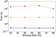
(a) BP

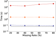
(b) FH

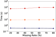
(c) MR

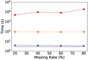
(d) SC

Figure 6. Decision - Running Time vs Missing Rates on Different Datasets (Uniform Perturbation)

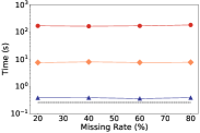
(a) BP

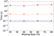
(b) FH

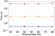
(c) MR

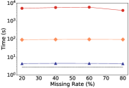
(d) SC

Figure 7. Decision - Running Time vs Missing Rates on Different Datasets (Feature Perturbation)

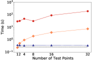
(a) BP

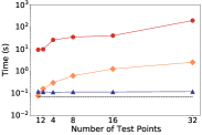
(b) FH

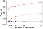
(c) MR

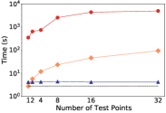
(d) SC

Figure 8. Decision - Running Time vs Number of Test Points on Different Datasets (Uniform Perturbation)

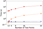
(a) BP

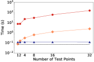
(b) FH

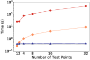
(c) MR

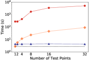
(d) SC

Figure 9. Decision - Running Time vs Number of Test Points on Different Datasets (Feature Perturbation)

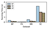
(a) Running Time

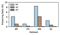
(b) Poisoning Rate

Figure 10. Data Poisoning—Running Time and Poisoning Rate on Different Datasets

6.3. Evaluation Results

For each dataset, we execute every algorithm $5$ times. For both the Decision Problem $\mathsf{CR\text{-}NaiveBayes}$ and Data Poisoning Problem $\mathsf{CR\text{-}NaiveBayes}^{\dagger}$, we report the average running time among the $5$ executions for fixed missing rate and the number of points. For $\mathsf{CR\text{-}NaiveBayes}^{\dagger}$, we additionally report the poisoning rate (for poisoning algorithms only), defined as the ratio between the number of cells marked as NULL by the data poisoning algorithm and the total number of cells in the dataset. As a general reference, the average training and prediction times of a single test point over each dataset FH, BP, MR and SC are $0.067$s, $0.253$s, $0.331$s and $2.812$s respectively, shown as black dashed lines on Figure 1-6 (i.e., Plain).

6.3.1. Decision Problems

To answer Q1, we first evaluate the running time of different decision algorithms (AD, Iterate and Iterate+Index) for $32$ test points on different datasets over varying missing rates from $20\%$ to $80\%$, with an increment of $20\%$. We also include the average running time of training and predicting a single test point for each original complete dataset, shown as Plain as a reference. Figure 6 and 7 present the running time over datasets obtained from Uniform Perturbation and Feature Perturbation respectively. We observe that Iterate+Index is almost $20\times$ faster than Iterate and much faster than the straightforward solution AD, which nonetheless does not have correctness guarantees. We can also see that the efficiency of Iterate+Index is robust against the missing rate in the datasets as the running time of our algorithms is almost uniform. Finally, comparing Figure 6 and 7 for the same dataset shows that the distribution of the missing cells in the dataset also does not affect the performance of our algorithms. We also remark that the running time of Iterate+Index and Plain are very similar but Iterate+Index decides whether a test point is certifiable robust, a much stronger guarantee compared to Plain with little extra cost on the running time. This shows that it is viable to efficiently apply certifiable robustness in practice to obtain much stronger guarantees in addition to the traditional ML pipeline.

We answer Q2 by running AD, Iterate and Iterate+Index on varying number of test points for each dataset. Figure 8 and 9 show the running time of each algorithm over datasets obtained from Uniform Perturbation and Feature Perturbation respectively, from $1$ test point to $32$ test points. We observe that the running time of AD and Iterate grows almost linearly with the number of test points, whereas the running time of Iterate+Index remains almost the same regardless of the number of test points. The initial offline index building introduced in the end of Section 3 can be slow to build at the beginning (see the sub-Figures when the number of test points is $1$), but its benefits are more apparent when the number of test points increases. For $32$ test points, we see that Iterate+Index outperforms Iterate by $10\times$.

In summary, Iterate+Index is a practical algorithm that can efficiently certify robustness for NBC for multiple test points and large datasets.

6.3.2. Data Poisoning Problem

We now present the evaluation results of different data poisoning algorithms for a single test point.

Our evaluations to answer Q1 are presented in Figure 10a. We see that the running time of OP is significantly faster than RP and marginally faster than SP. This is because SP uses the optimal strategies A1 and A2 as in OP, but not in the optimal sequence.

For Q3, Figure 10b presents the ratio between the number of poisoned cells and the total number of cells, called the poisoning rate. Note that RP always has a higher poisoning rate compared to SR and OP. Since OP is provably optimal, it has the smallest poisoning rate across all algorithms for the same dataset. Note that despite SP and OP have similar running times but their poisoning rate varies: This implies that the optimal strategies A1 and A2 are efficient to execute and the optimal sequence of applying A1 and A2 can minimize the number of poisoned cells drastically. Finally, note that OP achieves different poisoning rates for different datasets and the poisoning rates are often low. For example, the poisoning rate for FH is much lower than that for BP, showing that the dataset FH is more prone to a data poisoning attack than BP.

Overall, OP not only provides guarantees for finding the minimum number of poisoned cells, but also achieves the best performance in terms of running time. It also provides insights on the robustness of the dataset against data poisoning attacks.

7. Related Work

Data Cleaning. Cleaning the dirty data is the most natural resolution in the presence of dirty data. There has been a long line of research on data cleaning, such as error detection (Abedjan et al., 2016; Mahdavi et al., 2019), missing value imputation (Trushkowsky et al., 2013), and data deduplication (Chu et al., 2016). Multiple data cleaning frameworks have been developed (Wang et al., 2014a; Krishnan et al., 2016; Krishnan et al., 2017). For example, SampleClean (Wang et al., 2014a) introduces the Sample-and-Clean framework, which answers aggregate query by cleaning a small subset of the data. ActiveClean (Krishnan et al., 2016) is used to clean data for convex models which are trained by using gradient decent. BoostClean (Krishnan et al., 2017) selects data cleaning algorithms from pre-defined space. Moreover, there also exists some data cleaning frameworks by using knowledge bases and crowdsourcing (Bergman et al., 2015; Chu et al., 2015b). For instance, KATARA (Chu et al., 2015b) resolves ambiguity by using knowledge bases and crowdsourcing marketplaces. Furthermore, there have been efforts to accelerate the data cleaning process (Rekatsinas et al., 2017b; Chu et al., 2013; Chu et al., 2015a; Rezig et al., 2021; Yan et al., 2020).

Querying over Inconsistent Databases. Querying over inconsistent database has been studied for several decades. Consistent query answering is a principled approach to answer consistent answer from an inconsistent database violating from (Arenas et al., 1999). A long line of research has been dedicated to study this question from theoretical perspective (Libkin, 2011; Koutris and Suciu, 2012; Koutris and Wijsen, 2015). Recently, motivated by the previous works about relational query over incomplete database, CPClean (Karlaš et al., 2020) presents the concept of certain predicion, which connect the database theory and certifiable robustness in ML.

Certifiable Robustness in ML. Robust learning algorithms have received much attention recently. Robustness of decision tree under adversarial attack has been studied in (Chen et al., 2019; Vos and Verwer, 2021) and interests in certifying robust training methods have been observed (Shi et al., 2021). The notion of certain prediction, the synonym of certifiable robustness has been reinvented in (Karlaš et al., 2020) for connecting the certifiable robustness of Nearest Neighbor classifier to the downstream data cleaning task. Most recently, a more efficient algorithm for certifying the robustness of k-nearest neighbors are proposed in (Fan and Koutris, 2022). This paper studies the certifiable robustness for naive bayes classifiers and show the shortcomings of the data cleaning framework in CPClean (Karlaš et al., 2020).

Data Poisoning. Data poisoning attacks on machine learning has been studied for nearly a decade. A large number of work (Newell et al., 2014; Xiao et al., 2015; Mei and Zhu, 2015) shows that data poisoning can easily threaten the integrity of machine learning models. Many of these works focus on a specific class of models such as SVM and linear regression. There are many works proposing robust learning algorithms to defend against data poisoning (Steinhardt et al., 2017). Our work investigates how to attack the complete dataset to make test points certifiably non-robust.

8. Conclusion

We conclude this paper by identifying some open problems. It remains open to study the certifiable robustness of other widely used ML models such as random forests and gradient boosted trees. Additionally, it would be very helpful to design approximation algorithms with theoretical guarantees for $\#\mathsf{CR\text{-}NaiveBayes}$ and $\mathsf{CR\text{-}NaiveBayes}^{\dagger}$ for multiple test points. Finally, we envision that the insights gained from the study of certifiable robustness of different ML models would lead to more efficient data cleaning systems taking into consideration the downstream ML tasks.

Appendix A Proof of Theorem 5.4

We present a reduction from the VertexCover problem on $d$-regular graphs: Given a $d$-regular graph $G=(V,E)$ in which all vertices have degree $d$, find a set $S\subseteq V$ of minimum size such that every edge in $E$ is adjacent to some vertex in $S$.

Let $V=\{1,2,\dots,n\}$ and $m=|E|$. Assume without loss of generality that $G$ is not a clique. By the Brook’s theorem (Brooks, 1941), the $d$-regular graph $G$ is $d$-colorable. Let $\chi:V\rightarrow\{A_{1},A_{2},\dots,A_{d}\}$ be a $d$-coloring of $G$, which can be found in linear time.

Constructing $m$ test points. We first construct $m$ test points on attributes $A_{1},A_{2},\dots,A_{d}$ as follows: For each edge $\{u,v\}\in E$, introduce a test point $\bm{t}_{u,v}$ with values $u$ and $v$ at attributes $\chi(u)$ and $\chi(v)$, and a fresh integer value for all other attribute $A_{k}$ where $k\in\{1,2,\dots,d\}\setminus\{\chi(u),\chi(v)\}$.

It is easy to see that for two distinct edges $e=\{u,v\}$, $e^{\prime}=\{u^{\prime},v^{\prime}\}\in E$, if $e$ and $e^{\prime}$ do not share vertices, then $\bm{t}_{u,v}$ and $\bm{t}_{u^{\prime},v^{\prime}}$ do not agree on any attribute; and if they share a vertex $w$, then $\bm{t}_{u,v}$ and $\bm{t}_{u^{\prime},v^{\prime}}$ would agree on the attribute $\chi(w)$ with value $w$.

Note that to construct the test points, we used $n+(d-2)m$ domain values, $n$ for each vertex $V$ and $(d-2)m$ for all the fresh constants.

Constructing a clean dataset. For an attribute $A_{k}$, a domain value $u$ and a label $l$, we denote $p(A_{k},u,l)$ as a datapoint

$$p(A_{k},u,l):=(\square,\cdots,u,\cdots,\square),$$

with label $l$, in which the attribute $A_{k}$ has domain value $u$, and each $\square$ denotes a fresh domain value.

Let $M=n+(1+n/d)^{3}+1$ and $N=n+(d-2)m\cdot M$. We construct a dataset $\mathcal{D}$ of $2N$ points, in which $N$ points have label $l_{1}$, and $N$ points have label $l_{2}$ as follows.

• Datapoints with label $l_{1}$: for each domain value $u$ at attribute $A_{k}$, if $u\in V$, we introduce $p(A_{k},u,l_{1})$ once (and in this case, $A_{k}=\chi(u)$); or otherwise, we introduce $p(A_{k},u,l_{1})$ for $M$ times. It is easy to see that there are $N=n+(d-2)m\cdot M$ datapoints with label $l_{1}$.

• Datapoints with label $l_{2}$: for each domain value $u$ at attribute $A_{k}$, we introduce $p(A_{k},u,l_{2})$ once, and we introduce $N-M$ fresh datapoints of the form

  $$(\square,\square,\cdots,\square).$$

This construction can be done in polynomial time of $m$ and $n$. By construction, for each testpoint $\bm{t}_{u,v}=(c_{1},c_{2},\dots,c_{d})$, if $c_{k}\in V$, then the domain value $c_{k}$ occurs exactly once as a domain value of $A_{k}$, or otherwise $M$ times among all datapoints with label $l_{1}$; and $c_{k}$ occurs exactly once as a domain value of $A_{k}$ among all datapoints with label $l_{2}$.

Hence for each test point $\bm{t}_{u,v}$, $f_{\mathcal{D}}(\bm{t}_{u,v})=l_{1}$, by noting that

$$Pr(l_{1}\mid\bm{t}_{u,v})_{\mathcal{D}} =\frac{1}{Pr(\bm{t}_{u,v})_{\mathcal{D}}}\cdot\frac{1\cdot 1\cdot M^{d-2}}{N^{d}}\cdot\frac{N}{2N}$$

$$>\frac{1}{Pr(\bm{t}_{u,v})_{\mathcal{D}}}\cdot\frac{1\cdot 1\cdot 1^{d-2}}{N^{d}}\cdot\frac{N}{2N}$$

$$=Pr(l_{2}\mid\bm{t}_{u,v})_{\mathcal{D}}.$$

Now we argue that there is a vertex cover $S$ of $G$ with size at most $k$ if and only if we may alter at most $k$ missing values in $\mathcal{D}$ to obtain $\mathcal{D}^{\prime}$ such that for each point $\bm{t}_{u,v}$,

$$Pr(l_{1}\mid\bm{t}_{u,v})_{\mathcal{D}^{\prime}}<Pr(l_{2}\mid\bm{t}_{u,v})_{\mathcal{D}^{\prime}},$$

which yields $f_{\mathcal{D}}(\bm{t}_{u,v})\neq f_{\mathcal{D}^{\prime}}(\bm{t}_{u,v})$.

$\Longrightarrow$ Let $S\subseteq V$ be a vertex cover of $G$. Consider the dataset $\mathcal{D}^{\prime}$, obtained by altering for each $u\in S$ with $A_{k}=\chi(u)$, the datapoint

$$p(A_{k},u,l_{1})=(\square,\cdots,u,\cdots,\square)$$

into

$$(\square,\cdots,u^{\prime},\cdots,\square),$$

where $u^{\prime}\notin V$. For every test point $\bm{t}_{u,v}$, we argue that either $u$ does not occur at all at attribute $\chi(u)$, or $v$ does not occur at all at attribute $\chi(v)$ in $\mathcal{D}^{\prime}$. Indeed, since $S$ is a vertex cover, either $u\in S$ or $v\in S$, and thus either $p(\chi(u),u,l_{1})$ or $p(\chi(v),v,l_{1})$ is altered so that either $u$ or $v$ does not occur at all at attributes $\chi(u)$ or $\chi(v)$ in $\mathcal{D}^{\prime}$. Hence NBC would estimate that

$$Pr(l_{1}\mid\bm{t}_{u,v})_{\mathcal{D}^{\prime}}=0<\frac{1}{Pr(\bm{t}_{u,v})_{\mathcal{D}^{\prime}}}\cdot\frac{1}{N^{d}}\cdot\frac{N}{2N}=Pr(l_{2}\mid\bm{t}_{u,v})_{\mathcal{D}^{\prime}},$$

as desired.

$\Longleftarrow$ Assume that there is a dataset $\mathcal{D}^{\prime}$ with at most $k$ alternations to $\mathcal{D}$ such that $f_{\mathcal{D}}(\bm{t}_{u,v})=l_{1}$ but $f_{\mathcal{D}^{\prime}}(\bm{t}_{u,v})=l_{2}$ for every test point $\bm{t}_{u,v}$. It suffices to show that $G$ has a vertex cover of size at most $k$. Since $G$ must have a vertex cover of size $k\geq n$, we assume that $k<n$.

Consider an arbitrary test point

$$\bm{t}_{u,v}=(c_{1},c_{2},\dots,c_{n}).$$

We have that

$$Pr(l_{1}\mid\bm{t}_{u,v})_{\mathcal{D}^{\prime}}<Pr(l_{2}\mid\bm{t}_{1,2})_{\mathcal{D}^{\prime}}.$$

Let $x_{i}$ and $y_{i}$ be absolute value of the change of frequency from $\mathcal{D}$ to $\mathcal{D}^{\prime}$ of value $c_{i}$ for attribute $A_{i}$ in test points with labels $l_{1}$ and $l_{2}$ respectively. Then we have

(5) $$0\leq(1-x_{i})(1-x_{j})\cdot\prod_{k\in\{1,2,\dots,d\}\setminus\{i,j\}}(M-x_{k})<\prod_{1\leq k\leq d}(1+y_{k}).$$

We argue that without loss of generality, we can assume each $x_{i}$ and $y_{i}$ are nonnegative: if $y_{i}$ is negative, then right-hand-side of (5) is $0$ and cannot hold; and if $x_{i}$ is negative, i.e., the alternations increase the frequency of certain attributes among points with label $l_{1}$, then not performing such alterations would also preserve the inequality (5) with less than $k$ alterations.

Note that $x_{1}+x_{2}+\dots+x_{d}+y_{1}+y_{2}+\dots+y_{d}\leq k$.

For each test point $\bm{t}_{u,v}$, let $A_{i}=\chi(u)$ and $A_{j}=\chi(v)$, and we argue that we must have $x_{j}=1$ or $x_{j}=1$ (or both). Suppose for contradiction that $x_{i}=x_{j}=0$. Then, we have

$$\prod_{k\in\{1,2,\dots,d\}\setminus\{i,j\}}(M-x_{k}) =(1-x_{i})(1-x_{j})\cdot\prod_{k\in\{1,2,\dots,d\}\setminus\{i,j\}}(M-x_{k})$$

$$<\prod_{1\leq k\leq d}(1+y_{k})$$

$$\leq(1+\frac{y_{1}+y_{2}+\dots+y_{d}}{d})^{d}$$

$$\leq(1+\frac{n}{d})^{d}.$$

On the other hand, we have for each $k\in\{1,2,\dots,d\}\setminus\{i,j\}$, $x_{k}\leq n$, and thus

$$M-x_{k}\geq M-n>(1+\frac{n}{d})^{3}\geq(1+\frac{n}{d})^{\frac{d}{d-2}},$$

and it follows that

$$\prod_{k\in\{1,2,\dots,d\}\setminus\{i,j\}}(M-x_{k})\geq(1+\frac{n}{d})^{d},$$

a contradiction.

Now consider the set

$$S=\{u\mid A_{k}=\chi(u),x_{k}=1\}.$$

The set $S$ is a vertex cover, since for every edge $\{u,v\}\in E$, if the test point $\bm{t}_{u,v}$ has $A_{i}=\chi(u)$ and $A_{j}=\chi(v)$, we must have $x_{i}=1$ or $x_{j}=1$, and thus either $u\in S$ or $v\in S$. Since each $x_{k}=1$ correspond to an alteration, the size of $S$ is at most $k$.

The proof concludes by noting that both $\mathcal{D}$ and $\mathcal{D}^{\prime}$ are possible worlds of the incomplete dataset $\mathcal{D}^{\dagger}$ obtained by setting the altered cells in $\mathcal{D}^{\prime}$ from $\mathcal{D}$ as missing cells.

References

- (1)
- dat (2022a) 2022a. bodyPerformance Dataset. https://www.kaggle.com/kukuroo3/body-performance-data
- dat (2022b) 2022b. fetal_health Dataset. https://www.kaggle.com/andrewmvd/fetal-health-classification
- web (2022a) 2022a. Kaggle. https://www.kaggle.com/
- dat (2022c) 2022c. mushroom Dataset. https://www.kaggle.com/uciml/mushroom-classification
- web (2022b) 2022b. Sklearn. https://scikit-learn.org/stable/index.html
- dat (2022d) 2022d. star_classification Dataset. https://www.kaggle.com/fedesoriano/stellar-classification-dataset-sdss17
- Abedjan et al. (2016) Ziawasch Abedjan, Xu Chu, Dong Deng, Raul Castro Fernandez, Ihab F Ilyas, Mourad Ouzzani, Paolo Papotti, Michael Stonebraker, and Nan Tang. 2016. Detecting data errors: Where are we and what needs to be done? Proceedings of the VLDB Endowment 9, 12 (2016), 993–1004.
- Altowim et al. (2014) Yasser Altowim, Dmitri V. Kalashnikov, and Sharad Mehrotra. 2014. Progressive Approach to Relational Entity Resolution. Proc. VLDB Endow. 7, 11 (2014), 999–1010. https://doi.org/10.14778/2732967.2732975
- Arenas et al. (1999) Marcelo Arenas, Leopoldo Bertossi, and Jan Chomicki. 1999. Consistent query answers in inconsistent databases. In PODS.
- Bergman et al. (2015) Moria Bergman, Tova Milo, Slava Novgorodov, and Wang-Chiew Tan. 2015. Query-oriented data cleaning with oracles. In Proceedings of the 2015 ACM SIGMOD International Conference on Management of Data. 1199–1214.
- Bertossi et al. (2013) Leopoldo Bertossi, Solmaz Kolahi, and Laks VS Lakshmanan. 2013. Data cleaning and query answering with matching dependencies and matching functions. Theory of Computing Systems 52, 3 (2013), 441–482.
- Bohannon et al. (2007) Philip Bohannon, Wenfei Fan, Floris Geerts, Xibei Jia, and Anastasios Kementsietsidis. 2007. Conditional Functional Dependencies for Data Cleaning. In ICDE. IEEE Computer Society, 746–755.
- Brooks (1941) Rowland Leonard Brooks. 1941. On colouring the nodes of a network. In Mathematical Proceedings of the Cambridge Philosophical Society, Vol. 37. Cambridge University Press, 194–197.
- Chen et al. (2019) Hongge Chen, Huan Zhang, Si Si, Yang Li, Duane Boning, and Cho-Jui Hsieh. 2019. Robustness verification of tree-based models. arXiv:1906.03849 (2019).
- Cheng et al. (2008) Reynold Cheng, Jinchuan Chen, and Xike Xie. 2008. Cleaning uncertain data with quality guarantees. Proc. VLDB Endow. 1, 1 (2008), 722–735.
- Chu et al. (2016) Xu Chu, Ihab F Ilyas, and Paraschos Koutris. 2016. Distributed data deduplication. Proceedings of the VLDB Endowment 9, 11 (2016), 864–875.
- Chu et al. (2013) Xu Chu, Ihab F. Ilyas, and Paolo Papotti. 2013. Holistic data cleaning: Putting violations into context. In ICDE. IEEE Computer Society, 458–469.
- Chu et al. (2015a) Xu Chu, John Morcos, Ihab F. Ilyas, Mourad Ouzzani, Paolo Papotti, Nan Tang, and Yin Ye. 2015a. KATARA: A Data Cleaning System Powered by Knowledge Bases and Crowdsourcing. In SIGMOD Conference. ACM, 1247–1261.
- Chu et al. (2015b) Xu Chu, John Morcos, Ihab F Ilyas, Mourad Ouzzani, Paolo Papotti, Nan Tang, and Yin Ye. 2015b. Katara: A data cleaning system powered by knowledge bases and crowdsourcing. In Proceedings of the 2015 ACM SIGMOD international conference on management of data. 1247–1261.
- CloudLab (2018) CloudLab 2018. https://www.cloudlab.us/.
- Fan and Koutris (2022) Austen Z Fan and Paraschos Koutris. 2022. Certifiable Robustness for Nearest Neighbor Classifiers. arXiv:2201.04770 (2022).
- Karlaš et al. (2020) Bojan Karlaš, Peng Li, Renzhi Wu, Nezihe Merve Gürel, Xu Chu, Wentao Wu, and Ce Zhang. 2020. Nearest neighbor classifiers over incomplete information: From certain answers to certain predictions. arXiv:2005.05117 (2020).
- Khayyat et al. (2015) Zuhair Khayyat, Ihab F. Ilyas, Alekh Jindal, Samuel Madden, Mourad Ouzzani, Paolo Papotti, Jorge-Arnulfo Quiané-Ruiz, Nan Tang, and Si Yin. 2015. BigDansing: A System for Big Data Cleansing. In SIGMOD Conference. ACM, 1215–1230.
- Kohler and Link (2021) Henning Kohler and Sebastian Link. 2021. Possibilistic data cleaning. IEEE Transactions on Knowledge and Data Engineering (2021).
- Koutris and Suciu (2012) Paraschos Koutris and Dan Suciu. 2012. A dichotomy on the complexity of consistent query answering for atoms with simple keys. arXiv:1212.6636 (2012).
- Koutris and Wijsen (2015) Paraschos Koutris and Jef Wijsen. 2015. The data complexity of consistent query answering for self-join-free conjunctive queries under primary key constraints. In PODS.
- Krishnan et al. (2017) Sanjay Krishnan, Michael J Franklin, Ken Goldberg, and Eugene Wu. 2017. Boostclean: Automated error detection and repair for machine learning. arXiv preprint arXiv:1711.01299 (2017).
- Krishnan et al. (2016) Sanjay Krishnan, Jiannan Wang, Eugene Wu, Michael J Franklin, and Ken Goldberg. 2016. Activeclean: Interactive data cleaning for statistical modeling. Proceedings of the VLDB Endowment (2016).
- Libkin (2011) Leonid Libkin. 2011. Incomplete information and certain answers in general data models. In PODS.
- Mahdavi et al. (2019) Mohammad Mahdavi, Ziawasch Abedjan, Raul Castro Fernandez, Samuel Madden, Mourad Ouzzani, Michael Stonebraker, and Nan Tang. 2019. Raha: A configuration-free error detection system. In Proceedings of the 2019 International Conference on Management of Data. 865–882.
- Mei and Zhu (2015) Shike Mei and Xiaojin Zhu. 2015. Using machine teaching to identify optimal training-set attacks on machine learners. In AAAI.
- Newell et al. (2014) Andrew Newell, Rahul Potharaju, Luojie Xiang, and Cristina Nita-Rotaru. 2014. On the practicality of integrity attacks on document-level sentiment analysis. In Proceedings of the 2014 Workshop on Artificial Intelligent and Security Workshop.
- Peng et al. (2021) Jinglin Peng, Weiyuan Wu, Brandon Lockhart, Song Bian, Jing Nathan Yan, Linghao Xu, Zhixuan Chi, Jeffrey M Rzeszotarski, and Jiannan Wang. 2021. Dataprep. eda: task-centric exploratory data analysis for statistical modeling in python. In SIGMOD. 2271–2280.
- Prokoshyna et al. (2015) Nataliya Prokoshyna, Jaroslaw Szlichta, Fei Chiang, Renée J. Miller, and Divesh Srivastava. 2015. Combining Quantitative and Logical Data Cleaning. Proc. VLDB Endow. 9, 4 (2015), 300–311.
- Rekatsinas et al. (2017a) Theodoros Rekatsinas, Xu Chu, Ihab F Ilyas, and Christopher Ré. 2017a. Holoclean: Holistic data repairs with probabilistic inference. arXiv:1702.00820 (2017).
- Rekatsinas et al. (2017b) Theodoros Rekatsinas, Xu Chu, Ihab F. Ilyas, and Christopher Ré. 2017b. HoloClean: Holistic Data Repairs with Probabilistic Inference. Proc. VLDB Endow. 10, 11 (2017), 1190–1201.
- Rezig et al. (2021) El Kindi Rezig, Mourad Ouzzani, Walid G. Aref, Ahmed K. Elmagarmid, Ahmed R. Mahmood, and Michael Stonebraker. 2021. Horizon: Scalable Dependency-driven Data Cleaning. Proc. VLDB Endow. 14, 11 (2021), 2546–2554.
- Sahami et al. (1998) Mehran Sahami, Susan Dumais, David Heckerman, and Eric Horvitz. 1998. A Bayesian approach to filtering junk e-mail. In Learning for Text Categorization: Papers from the 1998 workshop, Vol. 62. Citeseer, 98–105.
- Shi et al. (2021) Zhouxing Shi, Yihan Wang, Huan Zhang, Jinfeng Yi, and Cho-Jui Hsieh. 2021. Fast certified robust training with short warmup. NeurIPS (2021).
- Steinhardt et al. (2017) Jacob Steinhardt, Pang Wei W Koh, and Percy S Liang. 2017. Certified defenses for data poisoning attacks. NIPS (2017).
- Trushkowsky et al. (2013) Beth Trushkowsky, Tim Kraska, Michael J Franklin, and Purnamrita Sarkar. 2013. Crowdsourced enumeration queries. In 2013 IEEE 29th International Conference on Data Engineering (ICDE). IEEE, 673–684.
- Vos and Verwer (2021) Daniël Vos and Sicco Verwer. 2021. Efficient Training of Robust Decision Trees Against Adversarial Examples. In ICML.
- Wang et al. (2014a) Jiannan Wang, Sanjay Krishnan, Michael J Franklin, Ken Goldberg, Tim Kraska, and Tova Milo. 2014a. A sample-and-clean framework for fast and accurate query processing on dirty data. In Proceedings of the 2014 ACM SIGMOD international conference on Management of data. 469–480.
- Wang et al. (2014b) Jiannan Wang, Sanjay Krishnan, Michael J. Franklin, Ken Goldberg, Tim Kraska, and Tova Milo. 2014b. A sample-and-clean framework for fast and accurate query processing on dirty data. In International Conference on Management of Data, SIGMOD 2014, Snowbird, UT, USA, June 22-27, 2014, Curtis E. Dyreson, Feifei Li, and M. Tamer Özsu (Eds.). ACM, 469–480. https://doi.org/10.1145/2588555.2610505
- Wang et al. (2007) Qiong Wang, George M Garrity, James M Tiedje, and James R Cole. 2007. Naive Bayesian classifier for rapid assignment of rRNA sequences into the new bacterial taxonomy. Applied and environmental microbiology 73, 16 (2007), 5261–5267.
- Xiao et al. (2015) Huang Xiao, Battista Biggio, Blaine Nelson, Han Xiao, Claudia Eckert, and Fabio Roli. 2015. Support vector machines under adversarial label contamination. Neurocomputing (2015).
- Yan et al. (2020) Jing Nathan Yan, Oliver Schulte, MoHan Zhang, Jiannan Wang, and Reynold Cheng. 2020. SCODED: Statistical constraint oriented data error detection. In SIGMOD. 845–860.