Detecting long-period variability in SDSS Stripe 82 standards catalog

Abstract

We report the results of a search for long-period ($100<P<600$ days) periodic variability in SDSS Stripe 82 standards catalog. The SDSS coverage of Stripe 82 enables such a search because there are on average 20 observations per band in $ugriz$ bands for about 1 million sources, collected over about 6 years, with a faint limit of $r\sim 22$ mag and precisely calibrated 1-2% photometry. We calculated the periods of candidate variable sources in this sample using the Lomb-Scargle periodogram and considered the three highest periodogram peaks in each of the $gri$ filters as relevant. Only those sources with $gri$ periods consistent within 0.1% were later studied. We use the Kuiper statistic to ensure uniform distribution of data points in phased light curves. We present 5 sources with the spectra consistent with quasar spectra and plausible periodic variability. This SDSS-based search bodes well for future sensitive large-area surveys, such as the Rubin Observatory Legacy Survey of Space and Time, which, due to its larger sky coverage (about a factor of 60) and improved sensitivity ($\sim 2$ mag), will be more powerful for finding such sources.

1 Introduction

Recent large-area time-domain sky surveys, such as the Optical Gravitational Lensing Experiment, (OGLE, Udalski et al., 1997; Udalski, 2003), the Catalina Real-Time Transient Survey (Drake et al., 2009), the Palomar Transient Factory (PTF, Law et al., 2009), Gaia (Gaia Collaboration et al., 2018, 2022), and the Zwicky Transient Facility (ZTF, Bellm et al., 2019) to name but a few, have shown the power of measuring variability of celestial sources for studying a variety of astrophysical phenomena. In this work we focus on one of the currently least well constrained poulations of astrophysical variability, the long-period, small-amplitude variability. The main reason why this domain of variability has not been studied in the past is the lack of adequate observational material: long observational baseline, photometric precision and depth over a large area of the sky are required to permit this kind of study.

There are several surveys that partially meet some the necessary requirements, however none of them bring them all together like Sloan Digital Sky Survey’s (SDSS) time-domain survey in the Stripe 82 (S82) region (described in detail in Section 2). This survey has photometric precision and depth (faint limit $r\sim 22$ mag) better than for example the Lincoln Near-Earth Asteroid Research (LINEAR, Stokes et al., 2000; Palaversa et al., 2013), Palomar Transient Factory (PTF, Law et al., 2009), Gaia (Gaia Collaboration et al., 2018) and Zwicky Transient Facility (ZTF, Bellm et al., 2019; Graham et al., 2019). Also, with on average $\sim$20 epochs in the $gri$ bands, it has more epochs than, Pan-STARRS (PS1, Chambers et al., 2016; Hernitschek et al., 2016) and Dark Energy Survey (DES, Dark Energy Survey Collaboration et al., 2016). The only surveys, other than SDSS S82, with which it is possible to study sources with a few percent change in brightness are Optical Gravitational Lensing Experiment (OGLE, Udalski et al., 1997; Udalski, 2003) and Kepler (Ciardi et al., 2011). The disadventage of OGLE over SDSS is in the fact that OGLE only observes the inner galactic bulge and the Magellanic Clouds. Similarly, SDSS covers a longer time span and a larger area of the sky than Kepler.

Our search for periodically variable objects in S82 was unbiased: we did not look for a specific type of variability, but aimed to utilise S82’s long observational baseline to discover any type of long-period variability. This could include both galactic and extragalactic sources. Possible galactic long-period candidates were multiperiodic, semi-regular variable red stars such as the OGLE Small Amplitude Red Giants (OSARGs) (Wray et al., 2004) and possibly some binary stars with edge-on orbits and nearly sinusoidal light curves. Periods of Mira stars also span the range of periods interesting to us, however, their large amplitudes would preclude them from becoming a part of the sample we analyzed, as large amplitude sources were already tagged in the S82 data by previous studies (see Section 2), and we specifically avoided those sources. It is possible, however, that some of the Miras in Stripe 82 were not detected in the earlier or our analysis. Both approaches depend on stable periodicity over the observational baseline for classification, which may not be the case for all Miras, who are known to exhibit period changes. We did not find any OSARGs and we could not confirm whether any OSARGs were indeed present in our sample as there is no overlap between OGLE surveys and the SDSS. We estimate that it would be difficult to identify OSARGs from the Stripe 82 data alone, given their multiperiodicity, small amplitudes and relatively sparse sampling of the Stripe 82 light curves. Extragalactic long-period variable candidates in this sample include quasars that may have a periodically varying optical light curve. The explanations of this behaviour include radio jet precession (e.g. Rieger, 2006; Kudryavtseva et al., 2011), tilted (warped) accretion disks (e.g. Tremaine & Davis, 2014), tidal distruption events (e.g. Liu et al., 2014) and supermassive binary black hole systems (e.g. Graham et al., 2015; Valtonen et al., 2008; Liu & Gezari, 2018). Our final sample of 5 candidates with convincing periodic behaviour consists of sources that have spectra consistent with quasar spectra.

Our paper is organized as follows: we describe the dataset used in our analysis in Section 2, report our analysis in Section 3, and discuss and summarize our results in Section 4.

2 SDSS Stripe 82 Imaging Data

One of the largest regions on the sky with multi-band photometry precise to about 0.01 mag, faint limit reaching $r\sim 22$, and $>10$ observations per object is a 300 deg² region known as the SDSS Stripe 82. Stripe 82 is a contiguous equatorial region that stretches between $-60^{\circ}\leq{\rm R.A.}\leq 60^{\circ}$ [20h to 4h], and $-1.266^{\circ}\leq{\rm Dec}\leq 1.266^{\circ}$. Following the initial concerted effort by the SDSS collaboration between 2001 and 2008 to map this region repeatedly to a forecast imaging depth, $r\leq 22$, several other surveys in various wavebands also have targeted this patch of sky to provide a rich multi-wavelength dataset suitable for a variety of investigations. SDSS observations too have continued in this region (e.g., the SDSS-II search for supernovae, Frieman et al., 2008), resulting in more epochs than initially planned.

Data from the SDSS imaging camera (Gunn et al., 1998) are collected in drift-scan mode, sequentially in each of the five Sloan filters in the order $riuzg$. The images that correspond to the same sky location in each of these five photometric bandpasses (these five images are collected over $\sim$5 minutes, with an exposure time of 54 seconds for each band) are grouped together for simultaneous processing as a field. A field is defined as a 36 seconds (1361 pixels) stretch of drift-scanning data from a single CCD column, referred as a camcol. Therefore, given this mode of data collection, the photometry in the $ugriz$ filters may be considered to be essentially simultaneous when interested in time scales of a day or longer.

2.1 The 2007 SDSS Standard Star Catalog

The SDSS standard star catalog published by Ivezić et al. (2007), hereafter I007 , was constructed by averaging multiple SDSS photometric observations (at least four per band, with a median of 10) in the $ugriz$ system. The catalog includes 1.01 million presumably non-variable unresolved objects. The averaged measurements for individual sources have random photometric errors below 0.01 mag for stars brighter than 19.5, 20.5, 20.5, 20, and 18.5 in $ugriz$, respectively (about twice better than for individual SDSS runs).

The 1.01 million standard stars in the I007 catalog were selected as non-variable sources by requiring that for each source their $\chi_{dof}^{2}<3$ ($\chi^{2}$ per degree of freedom) in each of the $gri$ bands, under the assumption of constant brightness. In addition, about 67,000 rejected light curves showed clear variability, with $\chi_{dof}^{2}$ per degree of freedom exceeding 3, and the root-mean-square (rms) variability exceeding 0.05 mag, in both $g$ and $r$ bands. The behavior of such obviously variable sources, dominated by RR Lyrae stars and quasars, was analyzed in detail by Sesar et al. (2007) and was not a part of this work.

Given that here we are interested in finding long periodic variability considering light curves for sources listed in the standard star catalog (i.e., those with $\chi^{2}<3$), the assumption is that the amplitudes of the sources found will be small. In other words, we aim to use periodogram analysis to uncover long-period variable sources with possible small-amplitudes that were not recognized as variable by I007. Furthermore, our final dataset includes more data than originally used by I007, as described next.

2.2 Post-2007 SDSS data

Recently, Thanjavur et al. (2021) extended light curves assembled by I007 with SDSS data obtained after 2007. Using the SDSS Data Release 15 (DR15) as available in April 2019 (Blanton et al., 2017), they constructed light curves for stars from the standard star catalog with about twice as many data points as available to I007 (about 20 on average and extending to 50 depending on the position within Stripe 82, see their Fig. 1). We note that DR15 does not include runs from the SDSS-II supernovae surveys (Frieman et al., 2008), which are typically of lower photometric quality. For more details, such as photometric recalibration of this new dataset, we refer the reader to Thanjavur et al. (2021).

The final dataset, consisting of all the light curves in the five $ugriz$ filters for the presumably 1,001,592 non-variable standard stars from the I007 catalog resulted in $\sim$20 GB of tabular data. This catalog is the starting point of our search for periodic variability. To make file search and access fast, the data have been organized into sub-directories, each spanning 1 $\deg$ in RA, and 0.1 $\deg$ in Dec (a "poor-man’s" two-dimensional tree structure). The light curves from this catalog are publicly available.

3 Light Curve Analysis

Since surveys mentioned earlier already explored the fast and large-amplitude variability in the S82 region, we focus on the long-period, small amplitude optical variations. We also show that the theoretical limit to which variability can be plausibly discovered with our data is at the level of A$\sim$0.03 mag in SDSS r-band.

We start with a sample of 1,001,592 light curves and select a subset of 143,505 light curves that have at least N = 25 observational epochs after filtering out epochs with likely spurious photometry. We identify the latter by having an epoch gri magnitude value outside the interval between 11 and 23 mag, or unrealistically small photometric errors (smaller than 0.0001 mag), or photometric errors larger than 0.2 mag. This minimum number of data points, together with photometric errors, implies the minimum variability amplitude that we can detect. In case of a source with constant brightness, and a light curve with at least 10 data points and reliably estimated photometric errors, the $\chi_{dof}^{2}$ distribution can be approximated as a Gaussian (normal) distribution with an expectation value of 1 and a standard deviation of $\sqrt{2/N}$. For illustration, for $N=25$ only about one non-variable source per thousand would have $\chi_{dof}^{2}>1.85$. Let us assume a hypothetical population of variable sources that represent, say, 0.01% of the sample, and have a variability amplitude $A$ that results in $\chi_{dof}^{2}$ distribution (under the assumption of no variability) with a median of 1.85. If now a subsample of all sources is selected with $\chi_{dof}^{2}>1.85$, it will include 95% of false positives (randomly scattered non-variable sources) and 5% of truly variable sources (i.e. 50% of all truly variable sources). Although the contamination rate is 19:1, let us assume here that a follow-up analysis can further “clean the sample”.

What is the variability amplitude $A$ that results in $\chi_{dof}^{2}$ distribution with a median of 1.85? It is easy to show that for a well sampled light curve following $y(t)=A\rm{sin}(\omega t)$ with homoscedastic Gaussian errors with standard deviation $\sigma$, the variance is $V=\sigma^{2}+A^{2}/2$ (Ivezić et al., 2019). The requirement that $\chi_{dof}^{2}=1.85$ yields a minimum detectable amplitude, $A=2.9\sigma/N^{1/4}=1.3\sigma$ for our requirement of N $\geq$ 25. Therefore, we expect that the completeness for truly variable sources when using selection $\chi_{dof}^{2}>1.85$ is at least 50% for $A\sim 0.03$ (using $\sigma\sim 0.02$ mag) and higher for larger values of $A$. In conclusion, we expect that our dataset is sensitive to amplitudes $A>$ 0.03 mag. According to Kepler results discussed by Ridgway et al. (2014), about 3% of stars are expected to show variability with $A>0.02$ mag (including non-periodic variables and for all values of period for periodic variables).

Search for periodicity should produce $\chi_{dof}^{2}\sim 1$ in case of truly periodic variables and thus yield a reduction of $\chi_{dof}^{2}$ by about a factor of two (or more in case of amplitudes larger than $\sim$0.03 mag). This reduction of $\chi_{dof}^{2}$ is the main method we employ here, but we supplement it with additional tests because the theoretical analysis above is sensitive to period aliasing and non-Gaussian behavior of photometric errors.

In the following subsections we outline our selection procedure.

3.1 Lomb-Scargle Periodogram analysis

For each of the 143,505 light curves, we computed Fast Lomb-Scargle periodograms (Press & Rybicki, 1989) using astropy implementation of the algorithm (Astropy Collaboration et al., 2013, 2018). The spacing of the search grid was selected automatically by the autopower method, which takes the user-supplied minimum and maximum frequencies as the input parameters ($f_{min}=1/600$ days^-1, $f_{max}=1/2$ days^-1) and adjusts the grid spacing according to the number of observations of the given source and the length of the observational baseline. This method will assign five grid points across each significant periodogram peak. The upper period search boundary was set to 600 days in order to limit the computational effort required to search for periods of approximately more than a hundred thousand sources. Lower period boundary was set to 2 days since periods of $P<1$ day would fall within the (short period) variable stars which have already been studied in detail in the SDSS S82 region by previous studies. Also, $P\sim 1$ day is strongly aliased so we moved lower limit up by a factor of two. Since $gri$ bands typically have the highest photometric signal-to-noise ratio (i.e. smallest photometric errors), we considered periodograms calculated using only the $gri$ data. We added a systematic photometric error of 0.01 mag in quadrature to photometric errors (uncertainties) reported by the SDSS photometric pipeline to avoid (rare) cases of unrealistically small reported errors.

In each band, we retained periods corresponding to the three highest periodogram peaks in order to have more options when validating possible contamination by aliasing. Taking more than three periodogram peaks would have typically sampled noise instead of the real signal. Given these nine periods per source, we select light curves with plausible periodic variability by requiring at least one period to be in common to each of the gri bands (to within 0.1%). Applying these constraints resulted in 1,078 unique sources with 2,135 corresponding periods.

3.2 $\chi^{2}$ analysis

For the selected 1,078 candidate periodic variable sources, we constructed phased light curves folded with the corresponding 2,135 periods. Then we checked how well the data agree with the sinusoidal light curve model by calculating $\chi^{2}$ and Lomb-Scargle periodogram in the following way:

$$P_{LS}=1-\frac{\chi^{2}_{per}}{\chi^{2}_{const}}.$$ (1)

Values $\chi^{2}_{per}$ and $\chi^{2}_{const}$ were calculated as:

$$\chi^{2}_{per}=\sigma_{G}\left(x_{per}\right)^{2},\mbox{ where: }x_{per}=\frac{mag-model}{magErr},$$ (2)

$$\chi^{2}_{const}=\sigma_{G}\left(x_{const}\right)^{2},\mbox{ where: }x_{const}=\frac{mag-\langle mag\rangle}{magErr}.$$ (3)

The used function $\sigma_{G}(x)=0.7413\cdot(x_{75}-x_{25})$ is the normalized interquartile range of the observed source magnitudes. We demanded $P_{LS}>0.5$, in other words we are requiring the improvement of the $\chi^{2}$ by the factor of 2. This requirement reduces the candidate sample to 342 unique sources with 601 periods.

Given the simple sinusoidal model that was used, it is possible that some sources with light curves significantly more complex than this model were rejected. However, during the analysis we also performed a visual verification of the candidate light curves and found no evidence of sources with more complex light curves.

3.3 Period analysis

From the period histogram in Figure 1 it is clear that there are a few period values that are recurring in Lomb-Scargle fits for different sources. It is natural to suspect that these periods are in fact aliases. Alternatively, this could mean we might have missed some true periods due to the coarseness of the grid selected by the autopower method applied by the Lomb-Scargle routine.

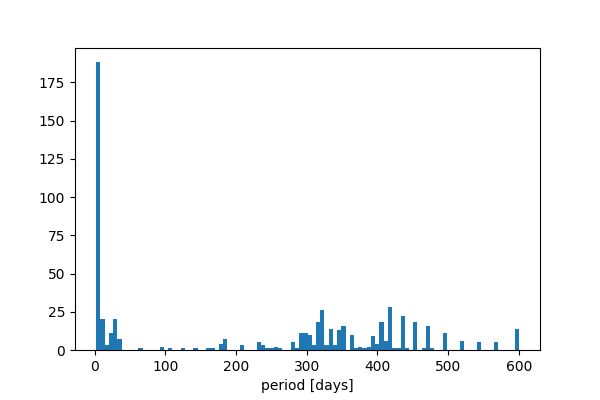
Figure 1: Histogram of periods for 342 sources with 601 corresponding periods.

To investigate the impact of using a sparse grid on the calculation of the periods, we re-ran the Lomb-Scargle period search on a denser grid. Since our sample was now much smaller than the one we started with, we were able to do it without demanding higher computational power. We used the same frequency range as before ($f_{min}=1/600$ days^-1, $f_{max}=1/2$ days^-1) and the grid was defined in the following way: for periods between 2 and 8 days, the time spacing ($\Delta t$) was 1 minute, for periods between 8 and 32 days $\Delta t$ was 3 minutes, for periods between 32 and 128 days $\Delta t$ was 10 minutes and for periods between 128 and 600 days $\Delta t$ was 1 hour. By comparing the results of the both period estimation runs, we were able to ascertain that no significant periodogram peaks were missed in the run with sparser period search grid. The Figure 2 shows an example of the comparison of periodograms obtained with a denser grid and with the autopower method. It is clear that there is no significant difference between them.

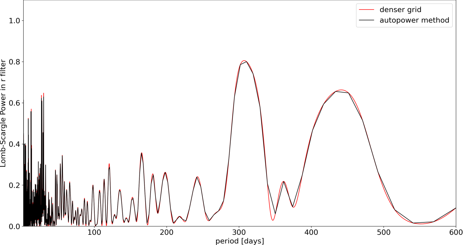
Figure 2: A typical example of a Lomb-Scargle periodogram for a candidate variable. Figure shows periodogram obtained using autopower method and the one calculated with a denser grid.

We discarded all of the (clustered) periods that can fit within a 0.1 day bin. Considering that these periods agree within 0.1 days, it is likely that they are aliases. That left us with 69 sources with 82 periods. For further analysis, we retained only objects with periods longer than 100 days. This boundary was applied in order to consider only long-period variability. Also, Figure 1 shows that most periods up to 100 days are grouped around small values (around zero). This is probably due to the 1-day aliasing caused by the Earth’s rotation. Furthermore, we have already mentioned that the catalog was previously cleaned of all short-period variable sources, so such cases were not considered in this work.

This constraint left us with 45 unique objects and 58 corresponding periods.

3.4 Phase distribution analysis

Further analysis was based on a requirement that every candidate should have a fairly uniform distribution of observations with respect to the phase. We base this requirement on the assumption that it is unlikely that for a significant fraction of the observed sources the cadence of the survey will be matched to the period of a particular source in a way that would produce observations that are always near the same point (or a few points) in the phased light curve. Indeed, given the uniformity of the cadence across all observed S82 fields, having a significant fraction of objects with clumped observations in the phased light curve would imply that those objects would have a common frequency $f_{c}\in f/n$, where $f$ is the period of the object and $n$ is a small integer. We note that with this requirement we may lose a fraction of good candidates, but since we are more concerned about purity of the sample than its completeness, every source whose phase-folded light curve exhibit clumping of observations was characterized as a false positive and eliminated from further analyses.

We quantify the uniformity of the distribution of the observed phases for each source using the Kuiper’s statistic. This statistic compares an empirical cumulative distribution function defined on a circle with the expected cumulative distribution function for a uniform distribution (CDF(x) = x). The maximum deviations are given as:

$$D=max(CDF_{data}-CDF_{unif})+max(CDF_{unif}-CDF_{data}).$$ (4)

We calculated the probability of obtaining the calculated D by a random fluctuation for a uniform distribution. When the probability is very small we conclude that we have non-uniform phase coverage, and therefore reject the corresponding period. D % for a uniform distribution, is a function of sample size, N: $D\%=\frac{C}{N^{p}}$, where for the case of 99.9 % we used $C=2.04$ and $p=0.486$, obtained by fitting this functional form to numerical simulations of draws from uniform distributions of varying size $8<N<10^{4}$, and valid for $0.95<D\%<0.999$. We only retained those that have $D<D_{99.9\%}$ in each of the $gri$ bands. After this filter, our sample decreased to 28 sources with 33 periods.

3.5 Source type determination and the determination of period uncertainties

In order to better characterise our final list of periodically variable sources, at this stage we used color-color and color-magnitude diagrams shown in Figure 3. The clustering observed in the upper left panel was a motivation for introducing 4 subgroups described in Table 1. For each source we introduce an ID based on the location in the $g$ vs $u-g$ plot in Figure 3.

Table 1: The division of the sample in 4 subgroups.

Regions	Types	ID
$i)$ u-g > 2.0	“late-type” K and M stars	0-1
$ii)$ 0.8 > u-g < 2.0	“intermediate-type” F and G stars	2-5
$iii)$ u-g < 0.8 and g < 20	quasars; possible presence of stars	6
$iv)$ u-g < 0.8 and g > 20	quasars	7-27

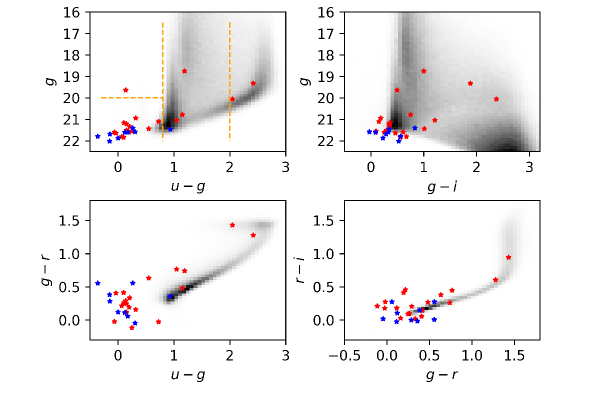
Figure 3: Color-magnitude and color-color diagrams for 28 candidates. Sources with period $P<365$ days are plotted as red and those with $P>365$ days are plotted as blue symbols. The gray background represents the distribution of all objects from the catalog.

3.5.1 Monte - Carlo simulations

We also preformed Monte - Carlo simulations to calculate the uncertainty of the estimated periods. The procedure and results are given in Appendix B. Using the results obtained with this method, we further filtered our sample. Requiring the agreement of previously calculated periods and those calculated by this method within the obtained uncertanty ($|P-P_{gatspy}|<\sigma_{P}$), our sample is reduced to 9 sources with 10 corresponding periods.

3.5.2 One-year period alias filtering

As a final filter, we check if the calculated periods are a real signals, or just aliases of one year. We used:

$$P_{a}=365\pm\frac{k}{n}\cdot 365;\ \ k=1,2;\ n=1,2,3,4,5,$$ (5)

to identify possible one-year aliases. If the calculated period P is within the range $P\pm\sigma_{P}$, where $\sigma_{P}$ is the period uncertainty obtained with simulations (the procedure is explained in Appendix B), we consider it an alias. Application of this filter left us with the final sample of 5 candidate periodically variable sources with 6 corresponding periods.

3.5.3 SDSS Cutouts

Since apparent variability in magnitude can be caused by a potential nearby source, we checked SDSS cutouts for each of the final 5 sources. By inspecting the images we confirmed that no candidates are affected by blending. An acceptable variable candidate should be isolated from all of the objects in its neighborhood.

3.5.4 Light Curves

In order to investigate the behavior of the light curves of each source at times different from those of the SDSS observations, we also searched the databases of other surveys. We found information about the light curves for the final 5 sources in ZTF DR11 (Masci et al., 2019) and Pan-STARRS (PS1, Chambers et al., 2016; Flewelling et al., 2020). We simultaneously plotted SDSS, ZTF and PS1 light curves in corresponding filters, along with the model. Our minimum requirement was that the apparent variability is confirmed in later times at least in one of the filters for at least one of the additional surveys. Apparent variability in additional surveys was confirmed for all 5 sources, which reduces the likelihood that the data from the original survey (SDSS) is bad data and that the detected (periodic) variability in SDSS is due to the random fluctuation.

4 Results

4.1 A summary of the applied filters and their effects on the selection.

Here we summarize the effect of each of the filters above on our selection procedure. We started with 143,505 light curves that have at least N =25.

• each of the $gri$ periods agree to within 0.1% $\rightarrow$ 1,078 sources with 2,135 corresponding periods

• $\chi^{2}$ and $P_{LS}>0.5$ analysis $\rightarrow$ 342 sources with 601 corresponding periods

• "repeated" periods ($\Delta P=0.1$ days) and periods 100 days < P < 600 $\rightarrow$ 45 sources with 58 corresponding periods

• Kuiper statistic: $D<D_{99.9\%}$ $\rightarrow$ 28 sources with 33 corresponding periods

• comparison with Monte-Carlo results $\rightarrow$ 9 sources with 10 corresponding periods

• one-year period alias $\rightarrow$ 5 sources with 6 corresponding periods
  
  Additional checks:

• blending $\rightarrow$ no sources were discarded

• comparison to more recent light curves $\rightarrow$ no sources were discarded

In the next section we proceed to analyze the remaining candidates.

4.2 Plausible periodically variable candidates

In order to better characterize our final sample we searched the SDSS DR16 online database for spectra of the candidate sources. We find that all 5 of the final candidates have a SDSS (Dawson et al., 2013, 2016) spectra consistent with quasar spectra. Their SDSS spectra are shown in Figure 4.

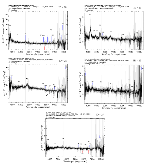
Figure 4: SDSS spectra for 5 periodically variable sources. All of them are consistent with quasar spectra.

All 5 sources have phased light curves with a uniform distribution of data points along the light curve, are well isolated from other sources and their (periodic) variability at later times is supported by either ZTF or PS1 survey data. The figures summarizing light curves of each of the sources, along with SDSS photometry cutouts are given in Appendix A.2.

Large uncertainties of the ZTF photometry prevent us from making any definitive arguments in case of the sources with IDs 10 and 25. However, PS1 photometry gives us sufficient variability confirmation in at least one of the bands. Source ID = 10 (Figure 5 a)) has the smallest amplitude ($A\sim 0.2$ mag) of all of the final candidates. ID = 25 (Figure 6 d) and e)) source has two reported periods that passed our selection criteria (P₁ = 300 d, P₂ = 299 d). Since they are within the uncertainty given in Table 3 ($|P_{1}-P_{2}|<\sigma_{P}$), we conclude that the same period is recovered by both methods (essentially 300 days).

Sources ID = 20, 27 boast a robust periodic variability confirmation by ZTF and PS1. Also, in Figure 5 b) and Figure 6 f) can be seen how ZTF amplitudes do not exclude SDSS-based model as being incorrect.

We single out a quasar with ID = 21 (Figure 5 c)) and P = 278 days as the most interesting one in this sample. Besides the optical variability detected in this work, this source also has Chandra X-ray catalog variability flag set to 1 (source displays flux variability within one or more observations, or between observations, in one or more energy bands) (Evans et al., 2010). For this source we performed an additional analysis of the periodicity with the 2D hybrid model (Kovačević et al., 2018, 2020), and found that this period and period calculated with the method explained in Section 3.1 are in excellent agreement. A detailed description of the procedure is given in Appendix C.

5 Summary and Conclusions

We report the results of a search for long-period variability in the SDSS Stripe 82 region. Starting with a sample of about million presumably constant sources we selected 5 as plausible candidates with periodic variability after a thorough analysis of their light curve characteristics and ancillary data. Our final sample consists of 5 sources with SDSS spectra consistent with quasar spectra. We consider our final candidates to be very likely to have periodic nature, although we cannot completely rule out the possibility of stochastic behavior causing the (apparently) periodic signal.

Determining the cause(s) of the variability of our candidates is not possible without additional data. Therefore, we singled out one quasar (ID=21) with a period of $P=278$ days whose periodic variability could not be excluded by ZTF and PS1, while its X-ray variability is detected by Chandra. Additional tests described in Appendix B and C included period estimations by a different models and used simulations to confirm reliability of the obtained results. Our simulations could not reject the assumption of periodicity of this quasar since its P-value is $\sim 60\%$. In order to further investigate the nature of its variability and possibly improve our approach to photometric detection of such sources in the context of detection exotic objects, and in particular gravitational wave emitters, we will be shortly obtaining Gemini GMOS-N spectra of the source.

We hope that this study provides to be useful in uncovering some of the long-period phenomena that may have been missed by the extant optical surveys. Although we initially expected long-period, low-amplitude stars in our final sample, we did not find them. Instead we found 5 excellent candidates for periodic variability displayed by spectroscopically confirmed quasars.

Appendix A Final candidates

In Table 2, we provide the spectral type as determined by the SDSS DR16 pipelines and a summary of photometric characteristics derived from the S82 photometry for the the final five candidates.

A.1 Table of final candidates

Table 2: Table of 5 long-period small-amplitude variability candidates.

objID	ID	SPECTRAL  TYPE	ra	dec	period	u	g	r	i	z	u-g	g-r	Amp(g)	Amp(r)	Amp(i)
1237666338651242745	10	QSO	14.629833	-0.622042	297.1988	21.30	21.18	20.93	20.84	20.4	0.12	0.25	0.28	0.27	0.22
1237666338653864147	20	QSO	20.57287	-0.422368	466.3183	21.69	21.39	21.26	21.36	20.68	0.30	0.13	1.22	1.08	0.97
1237666408438038843	21	QSO	350.059098	0.416449	277.8278	21.45	21.51	21.13	21.08	20.76	-0.06	0.38	0.63	0.52	0.44
1237663783133970736	25	QSO	23.53744	-0.839078	299.7779	21.90	21.79	21.38	21.21	20.58	0.11	0.41	0.34	0.33	0.29
1237666300553068800	27	QSO	44.539858	-0.206044	479.5917	21.81	21.73	21.43	21.32	20.71	0.08	0.30	1.13	0.96	0.82

A.2 Representative figures of final candidates

Here we summarize all the plausible periodically variable candidates represented by two panels that were used during our analyses.

Each figure contains:

• Left column: SDSS cutouts described in Section 3.5.3,

• Middle column: light curves in $ugriz$ bands with light- curve model derived using SDSS data. In addition to SDSS data, ZTF and PS1 data are also plotted in the figure to check whether the variability can be confirmed at later times with additional surveys. To account for the difference between the instruments, a simple magnitude correction was applied to each of the $gri$ filters:

  $$SURVEY_{corr}=SURVEY+\langle SURVEY\rangle-\langle SDSS\rangle,$$ (A1)

  where $SURVEY_{corr}$ is the corrected magnitude, i.e. magnitude shifted by the median difference between the survey in question and the SDSS ($\langle SURVEY\rangle-\langle SDSS\rangle$).

  In some cases few ZTF and PS1 data points are not visible in the figures because their difference with respect to the model light curve is too large. In order to preserve convenient scaling of the plots, we left these outlying values outside the range of the plots and instead designated them with an arrow on the left-hand side in some of the panels in the middle column. The arrows are color-coded according to the survey and the arrows’ length ($l$) is proportional to the number of data points ($N$) outside the ordinate range, with: $l=N\cdot 0.05+0.03$. Furthermore, given the shallower ZTF limiting magnitudes with respect to Pan-STARRS and SDSS ( 20.5 mag), and consequently larger scatter at the ZTF’s faint end, we binned the ZTF data in 7-day intervals and calculated a weighted mean magnitude for each bin in order to improve photometric precision and enhance the legibility of the plots.

• Right column: phased light curves in $ugriz$ bands.

Figure 5: Variable candidates.

Figure 6: Variable candidates.

Appendix B Results of Monte Carlo simulations

The reliability of the chosen period-finding procedure has been verified by comparing the derived periods to the multiband model and by employing Monte Carlo simulations. To this end, we have chosen to use the multiband extension of the Lomb-Scargle algorithm.

We have chosen the algorithm implemented in the gatspy package (VanderPlas & Ivezić, 2015). The multiband periodogram extends the Lomb-Scargle period finding algorithm by treating multiband observations as a dataset with a categorical variable for the observed band. The model uses a single fitting procedure for all observed bands, constructed by including a set of Lomb-Scargle model parameters for each band.

We have employed Monte Carlo simulations to estimate the reliability of the derived periods. We base our simulations on the best-fitting gatspy light curve model of magnitudes $m$, observed at time $t$ and in the band $b$, $m(t,b)$. A particular mock observation, $i$, consists of a simulated point: $(t_{i},b_{i},m_{i},\sigma_{m,i})$. Instead of taking a simple bootstrap that would only reshuffle the dataset, we employed the Gaussian kernel density estimator (KDE) to first determine the distributions of $t$, $m$, and $\sigma_{m}$, and then to draw a random point from these distributions. This procedure produced mock lightcurves that consisted of the same number of points as the original dataset. The data points were assumed to be independently distributed among the different bands, with each band appearing as many times in the mock lightcurve as in the original lightcurve. When choosing the optimal KDE distributions, we found that the magnitude error distribution is best reproduced when estimating $\log\sigma_{m}$ using KDE instead of estimating the KDE of $\sigma_{m}$ (see Tisanić et al., in prep). The magnitudes at a particular mock time were computed by fitting the multiband Lomb-Scargle function to the original dataset, computing its prediction at the mock time (and for the chosen randomly-selected band), and then by adding to this value the value of the simulated error $\sigma_{m}$.

We drew 1000 random lightcurves per object and set the number of mock times to the number of observing times in the original light curves. The gatspy multiband periodogram has been run on each mock dataset to estimate the reliability of the derived periods. We employed the robust method of deriving the standard deviations of the period distributions using the 16th and the 84th percentiles of the simulated period distributions. We then computed the P-values based on the estimated sigma value and our periods fitted using the astropy implementation of the Lomb-Scargle periodogram derived in the main body of this work, labeled as expected P-values in Table 3. Since a portion of the standard deviations were smaller than one day, we capped the standard deviations used for computing the P-values to 0.1 days.

Table 3: Results of Monte Carlo simulations of the sample’s periods.

ID	$\sigma_{P}$	expected period with errors	gatspy period with errors	simulated period with errors	expected P-value ($\sigma\to\mathrm{max}(\sigma,0.1d$))	gatspy P-value ($\sigma\to\mathrm{max}(\sigma,0.1d$))
10	2	297 $\pm$ 2	296 $\pm$ 2	296 $\pm$ 2	0.66	0.99
20	2	466 $\pm$ 2	467 $\pm$ 2	466 $\pm$ 2	0.73	0.56
21	1	278 $\pm$ 1	278 $\pm$ 1	278 $\pm$ 1	0.60	0.99
25	2	300 $\pm$ 2	302 $\pm$ 2	302 $\pm$ 2	0.21	0.92
27	3	480 $\pm$ 3	479 $\pm$ 3	478 $\pm$ 3	0.45	0.56

Appendix C Results of 2D Hybrid method

In general random fluctuations account for a significant portion of the variance in time series, so that the amplitudes of these stochastic effects are seen to be greater on longer periods. Due to the fact that the spectral density of red noise is inversely related to frequency, the red noise has a particularly significant impact on the lower frequencies. Thus to cope with this challenge, we also applied time domain periodicity search called 2D Hybrid method which relies on different types of wavelets (Kovačević et al., 2018, 2019). Given two time series $y_{t}$ and $y^{\prime}_{t}$, we can compare their wavelet matricies (scalograms) $\mathcal{S}$ and $\mathcal{S}^{\prime}$ in order to know if they follow similar patterns. Our 2D Hybrid method uses correlation as a comparison of scalograms (Kovačević et al., 2020). The 2D Hybrid approach employs various wavelets, e.g. continous, discrete, Weighted Wavelet Z-transform-WWZ (Foster, 1996), high-resolution superlets (Moca et al., 2021), and both observed light curves and their models. The method generates a contour map of the intensity of (auto) correlation on a period-period plane defined by two independent period axes matching to the two time series (or one). The map is symmetric and can be integrated along any of the axes, yielding in a periodogram-like curve of the strength of correlation among oscillations (for more details see Kovačević et al., 2018, 2019).

The significance of a detected period $\sigma_{P}$, we calculated by shuffling of time series (Johnson et al., 2019) so that the period was recomputed over this new modified data set and the height of the maximum peak in 2D Hybrid integrate map was compared to that found for the original simulated data. This process was repeated N (e.g. 100, as the wavelet computation) times and the significance level was then determined as (Johnson et al., 2019):

$$\sigma_{P}=\frac{x}{N}$$ (C1)

where $x$ represents the number of times that the peak power of the period in the original data was greater than that of the uncorrelated ensemble.

We also used another approach for estimating significance which is based on moving block bootstrap (MBB) methodology (Ivezic et al., 2014; Suveges, 2012; VanderPlas, 2018). In MBB apporach, blocks of data of a given length are glued together to create a new time series. Similarly to shuffling method, we first calculated periods of bootstraped mock light curves. Then the Generalized extreme value (GEV) distribution is fitted to the histogram of detected peaks in mock curves. For a given range of significance levels (p-values) we obtain the associated confidence level from the fitted GEV. If the candidate period has a peak value greater than the confidence level then we can reject the null hypothesis that the observed light curve is not periodic with given significance level.

Applying our 2D Hybrid method which core is the WWZ, we obtained period of $278.36^{57.34}_{-25.21}$ days, and significance above 99% measured by shuffling method, whereas GEV approach produces significance of 90%. In order to apply the 2D hybrid method with the high-resolution superlets core, we need homogenous data. Thus we modeled observed light curve with Deep Gaussian process (see e.g. Damianou & Lawrence, 2013) consisting of latent variable layer and two gaussian process layers. The Gaussian processes have Matern₁₂ and Matern₃₂ kernels. Detected period is $288.62^{+28.84}_{-07.35}$ days, with significances of 95% based on shuffling method and 88% based on MBB.

References

- Astropy Collaboration et al. (2013) Astropy Collaboration, Robitaille, T. P., Tollerud, E. J., et al. 2013, A&A, 558, A33, doi: 10.1051/0004-6361/201322068
- Astropy Collaboration et al. (2018) Astropy Collaboration, Price-Whelan, A. M., Sipőcz, B. M., et al. 2018, AJ, 156, 123, doi: 10.3847/1538-3881/aabc4f
- Bellm et al. (2019) Bellm, E. C., Kulkarni, S. R., Graham, M. J., et al. 2019, PASP, 131, 018002, doi: 10.1088/1538-3873/aaecbe
- Blanton et al. (2017) Blanton, M. R., Bershady, M. A., Abolfathi, B., et al. 2017, AJ, 154, 28, doi: 10.3847/1538-3881/aa7567
- Chambers et al. (2016) Chambers, K. C., Magnier, E. A., Metcalfe, N., et al. 2016, ArXiv e-prints. https://arxiv.org/abs/1612.05560
- Ciardi et al. (2011) Ciardi, D. R., von Braun, K., Bryden, G., et al. 2011, AJ, 141, 108, doi: 10.1088/0004-6256/141/4/108
- Damianou & Lawrence (2013) Damianou, A., & Lawrence, N. 2013, in Proceedings of the Sixteenth International Workshop on Artificial Intelligence and Statistics (AISTATS), ed. C. Carvalho & P. Ravikumar, AISTATS ’13 (JMLR W&CP 31), 207–215
- Dark Energy Survey Collaboration et al. (2016) Dark Energy Survey Collaboration, Abbott, T., Abdalla, F. B., et al. 2016, MNRAS, 460, 1270, doi: 10.1093/mnras/stw641
- Dawson et al. (2013) Dawson, K. S., Schlegel, D. J., Ahn, C. P., et al. 2013, AJ, 145, 10, doi: 10.1088/0004-6256/145/1/10
- Dawson et al. (2016) Dawson, K. S., Kneib, J.-P., Percival, W. J., et al. 2016, AJ, 151, 44, doi: 10.3847/0004-6256/151/2/44
- Drake et al. (2009) Drake, A. J., Djorgovski, S. G., Mahabal, A., et al. 2009, ApJ, 696, 870, doi: 10.1088/0004-637X/696/1/870
- Evans et al. (2010) Evans, I. N., Primini, F. A., Glotfelty, K. J., et al. 2010, ApJS, 189, 37, doi: 10.1088/0067-0049/189/1/37
- Flewelling et al. (2020) Flewelling, H. A., Magnier, E. A., Chambers, K. C., et al. 2020, ApJS, 251, 7, doi: 10.3847/1538-4365/abb82d
- Foster (1996) Foster, G. 1996, AJ, 112, 1709, doi: 10.1086/118137
- Frieman et al. (2008) Frieman, J. A., Bassett, B., Becker, A., et al. 2008, AJ, 135, 338, doi: 10.1088/0004-6256/135/1/338
- Gaia Collaboration et al. (2018) Gaia Collaboration, Brown, A. G. A., Vallenari, A., et al. 2018, A&A, 616, A1, doi: 10.1051/0004-6361/201833051
- Gaia Collaboration et al. (2022) Gaia Collaboration, Vallenari, A., Brown, A. G. A., et al. 2022, arXiv e-prints, arXiv:2208.00211. https://arxiv.org/abs/2208.00211
- Graham et al. (2015) Graham, M. J., Djorgovski, S. G., Stern, D., et al. 2015, Nature, 518, 74, doi: 10.1038/nature14143
- Graham et al. (2019) Graham, M. J., Kulkarni, S. R., Bellm, E. C., et al. 2019, PASP, 131, 078001, doi: 10.1088/1538-3873/ab006c
- Gunn et al. (1998) Gunn, J. E., Carr, M., Rockosi, C., et al. 1998, AJ, 116, 3040, doi: 10.1086/300645
- Hernitschek et al. (2016) Hernitschek, N., Schlafly, E. F., Sesar, B., et al. 2016, ApJ, 817, 73, doi: 10.3847/0004-637X/817/1/73
- Hunter (2007) Hunter, J. D. 2007, Computing In Science & Engineering, 9, 90, doi: 10.1109/MCSE.2007.55
- IRSA (2022) IRSA. 2022, Time Series Tool, IPAC, doi: 10.26131/IRSA538
- Ivezic et al. (2014) Ivezic, v., Connolly, A. J., VanderPlas, J. T., & Gray, A. 2014, Statistics, Data Mining, and Machine Learning in Astronomy: A Practical Python Guide for the Analysis of Survey Data (Princeton University Press), doi: 10.23943/princeton/9780691151687.001.0001
- Ivezić et al. (2019) Ivezić, Ž., Connelly, A. J., Vanderplas, J. T., & Gray, A. 2019, Statistics, Data Mining, and Machine Learning in Astronomy
- Ivezić et al. (2007) Ivezić, Ž., Smith, J. A., Miknaitis, G., et al. 2007, The Astronomical Journal, 134, 973, doi: 10.1086/519976
- Johnson et al. (2019) Johnson, M. A. C., Gandhi, P., Chapman, A. P., et al. 2019, MNRAS, 484, 19, doi: 10.1093/mnras/sty3466
- Jones et al. (2001–) Jones, E., Oliphant, T., Peterson, P., et al. 2001–, SciPy: Open source scientific tools for Python. http://www.scipy.org/
- Kovačević et al. (2018) Kovačević, A. B., Pérez-Hernández, E., Popović, L. Č., et al. 2018, MNRAS, 475, 2051, doi: 10.1093/mnras/stx3137
- Kovačević et al. (2020) Kovačević, A. B., Popović, L. Č., & Ilić, D. 2020, Open Astronomy, 29, 51, doi: 10.1515/astro-2020-0007
- Kovačević et al. (2019) Kovačević, A. B., Popović, L. Č., Simić, S., & Ilić, D. 2019, ApJ, 871, 32, doi: 10.3847/1538-4357/aaf731
- Kudryavtseva et al. (2011) Kudryavtseva, N. A., Britzen, S., Witzel, A., et al. 2011, A&A, 526, A51, doi: 10.1051/0004-6361/201014968
- Law et al. (2009) Law, N. M., Kulkarni, S. R., Dekany, R. G., et al. 2009, PASP, 121, 1395, doi: 10.1086/648598
- Liu et al. (2014) Liu, F. K., Li, S., & Komossa, S. 2014, ApJ, 786, 103, doi: 10.1088/0004-637X/786/2/103
- Liu & Gezari (2018) Liu, T., & Gezari, S. 2018, in American Astronomical Society Meeting Abstracts, Vol. 231, American Astronomical Society Meeting Abstracts #231, 105.02
- Masci et al. (2019) Masci, F. J., Laher, R. R., Rusholme, B., et al. 2019, PASP, 131, 018003, doi: 10.1088/1538-3873/aae8ac
- Moca et al. (2021) Moca, V. V., Bârzan, H., Nagy-Dăbâcan, A., & Mure\textcommabelowsan, R. C. 2021, Nature communications, 12, 1
- Oliphant (2006) Oliphant, T. E. 2006, A guide to NumPy, Vol. 1 (Trelgol Publishing USA)
- Palaversa et al. (2013) Palaversa, L., Ivezić, Ž., Eyer, L., et al. 2013, AJ, 146, 101, doi: 10.1088/0004-6256/146/4/101
- Press & Rybicki (1989) Press, W. H., & Rybicki, G. B. 1989, ApJ, 338, 277, doi: 10.1086/167197
- Ridgway et al. (2014) Ridgway, S. T., Matheson, T., Mighell, K. J., Olsen, K. A., & Howell, S. B. 2014, ApJ, 796, 53, doi: 10.1088/0004-637X/796/1/53
- Rieger (2006) Rieger, F. M. 2006, in Populations of High Energy Sources in Galaxies, ed. E. J. A. Meurs & G. Fabbiano, Vol. 230, 239–240, doi: 10.1017/S1743921306008313
- Sesar et al. (2007) Sesar, B., Ivezić, Ž., Lupton, R. H., et al. 2007, AJ, 134, 2236, doi: 10.1086/521819
- Stokes et al. (2000) Stokes, G. H., Evans, J. B., Viggh, H. E. M., Shelly, F. C., & Pearce, E. C. 2000, Icarus, 148, 21, doi: 10.1006/icar.2000.6493
- Suveges (2012) Suveges, M. 2012, in Seventh Conference on Astronomical Data Analysis, ed. J.-L. Starck & C. Surace, 16
- Thanjavur et al. (2021) Thanjavur, K., Ivezić, Ž., Allam, S. S., et al. 2021, MNRAS, 505, 5941, doi: 10.1093/mnras/stab1452
- Tremaine & Davis (2014) Tremaine, S., & Davis, S. W. 2014, MNRAS, 441, 1408, doi: 10.1093/mnras/stu663
- Udalski (2003) Udalski, A. 2003, Acta Astron., 53, 291. https://arxiv.org/abs/astro-ph/0401123
- Udalski et al. (1997) Udalski, A., Kubiak, M., & Szymanski, M. 1997, Acta Astron., 47, 319. https://arxiv.org/abs/astro-ph/9710091
- Valtonen et al. (2008) Valtonen, M. J., Lehto, H. J., Nilsson, K., et al. 2008, Nature, 452, 851, doi: 10.1038/nature06896
- VanderPlas et al. (2012) VanderPlas, J., Connolly, A. J., Ivezić, Ž., & Gray, A. 2012, in Proceedings of Conference on Intelligent Data Understanding (CIDU), pp. 47-54, 2012., 47–54, doi: 10.1109/CIDU.2012.6382200
- VanderPlas (2018) VanderPlas, J. T. 2018, ApJS, 236, 16, doi: 10.3847/1538-4365/aab766
- VanderPlas & Ivezić (2015) VanderPlas, J. T., & Ivezić, Ž. 2015, ApJ, 812, 18, doi: 10.1088/0004-637X/812/1/18
- Wray et al. (2004) Wray, J. J., Eyer, L., & Paczyński, B. 2004, MNRAS, 349, 1059, doi: 10.1111/j.1365-2966.2004.07587.x