Investigating the complexity of the double distance problems
Abstract
Two genomes and over the same set of gene families form a canonical pair when each of them has exactly one gene from each family. Different distances of canonical genomes can be derived from a structure called breakpoint graph, which represents the relation between the two given genomes as a collection of cycles of even length and paths. Let and be the numbers of cycles of length and of paths of length , respectively. Furthermore, let be the number of common genes of genomes and . Then, the breakpoint distance of and is equal to . Similarly, when the considered rearrangements are those modeled by the double-cut-and-join (DCJ) operation, the rearrangement distance of and is , where is the total number of cycles and is the total number of paths of even length.
The distance formulation is a basic unit for several other combinatorial problems related to genome evolution and ancestral reconstruction, such as median or double distance. Interestingly, both median and double distance problems can be solved in polynomial time for the breakpoint distance, while they are NP-hard for the rearrangement distance. One way of exploring the complexity space between these two extremes is to consider a distance, defined to be , and increasingly investigate the complexities of median and double distance for the distance, then the distance, and so on. While for the median much effort was done in our and in other research groups but no progress was obtained even for the distance, for solving the double distance under and distances we could devise linear time algorithms, which we present here.
Keywords:
Comparative genomics, Genome rearrangement, breakpoint distance, double-cut-and-join (DCJ) distance, double distance.1 Introduction
In genome comparison, the most elementary problem is that of computing a distance between two given genomes [San92], each one being a set of chromosomes. Usually a high-level view of a chromosome is adopted, in which each chromosome is represented by a sequence of oriented genes and the genes are classified into families. The simplest model in this setting is the breakpoint model, whose distance consists of somehow quantifying the distinct adjacencies between the two genomes, an adjacency in a genome being the oriented neighborhood between two genes in one of its chromosomes [TAN-ZHE-SAN-2009]. Other models rely on large-scale genome rearrangements, such as inversions, translocations, fusions and fissions, yielding distances that correspond to the minimum number of rearrangements required to transform one genome into another [HAN-PEV-1995, HAN-PEV-1999, YAN-ATT-FRI-2005].
Independently of the underlying model, the distance formulation is a basic unit for several other combinatorial problems related to genome evolution and ancestral reconstruction [TAN-ZHE-SAN-2009]. The median problem, for example, has three genomes as input and asks for an ancestor genome that minimizes the sum of its distances to the three given genomes. Other models are related to the whole genome duplication (WGD) event [ELM-SAN-2003]. Let the doubling of a genome duplicate each of its chromosomes. The double distance is the problem that has a duplicated genome and a singular genome as input and computes the distance between the former and a doubling of the latter. The halving problem has a duplicated genome as input and asks for a singular genome whose double distance to the given duplicated genome is minimized. Finally, the guided halving problem has a duplicated and a singular genome as input and asks for another singular genome that minimizes the sum of its double distance to the given duplicated genome and its distance to the given singular genome.
Our study relies on the breakpoint graph, a structure that represents the relation between two given genomes [BAF-PEV-1993]. When the two genomes are over the same set of gene families and form a canonical pair, that is, when each of them has exactly one gene from each family, their breakpoint graph is a collection of cycles of even length and paths. Assuming that both genomes have genes, if we call -cycle a cycle of length and -path a path of length , the corresponding breakpoint distance is equal to , where is the number of 2-cycles and is the number of 0-paths [TAN-ZHE-SAN-2009]. Similarly, when the considered rearrangements are those modeled by the double-cut-and-join (DCJ) operation [YAN-ATT-FRI-2005], the rearrangement distance is , where is the total number of cycles and is the total number of even paths [BER-MIX-STO-2006].
While the halving problem under both breakpoint and rearrangement distances can be solved in polynomial time [TAN-ZHE-SAN-2009, ELM-SAN-2003, ALE-PEV-2008, MIX-2008], median, double distance and guided halving problems can be solved in polynomial time only under the breakpoint distance, but are NP-hard under the rearrangement distance [TAN-ZHE-SAN-2009]. One way of exploring the complexity space between these two extremes is to consider a distance [Chauve2018], defined to be , and increasingly investigate the complexities of median, guided halving and double distance under the distance, then under the distance, and so on. Note that the distance is the breakpoint distance and the distance is the DCJ distance. To the best of our knowledge, the guided halving problem has not been studied for this class of problems, while for the median under distance much effort has been done in our group and in other research groups (e.g. [Chauve2018]) but no progress was obtained so far.
In contrast, for the double distance, while and higher were not yet studied, we succeeded in devising efficient algorithms for and . Our results, which we present here, are built on a variation of the breakpoint graph, called ambiguous breakpoint graph [TAN-ZHE-SAN-2009] and have three main parts. First we show that in any double distance, including the NP-hard DCJ double distance, all 2-cycles and 0-paths are fulfilled, meaning that the common adjacencies and common telomeres between the compared genomes are always conserved. Then we show that the double distance can be computed by a greedy linear time algorithm. Finally we present a non-greedy but still linear time algorithm for the double distance.
This paper is an extended version of our two recent works [BBKS2022, BBKS2023].
2 Background
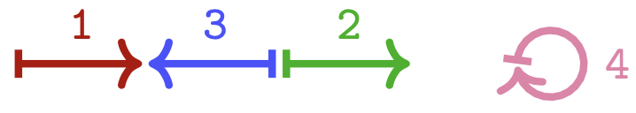
A chromosome is an oriented DNA molecule and can be either linear or circular. We represent a chromosome by its sequence of genes, where each gene is an oriented DNA fragment. We assume that each gene belongs to a family, which is a set of homologous genes. A gene that belongs to a family is represented by the symbol itself if it is read in forward orientation or by the symbol if it is read in reverse orientation. For example, the sequences and represent, respectively, a linear (flanked by square brackets) and a circular chromosome (flanked by parentheses), both shown in Figure 1, the first composed of three genes and the second composed of a single gene. Note that if a sequence represents a chromosome , then can be equally represented by the reverse complement of , denoted by , obtained by reversing the order and the orientation of the genes in . Moreover, if is circular, it can be equally represented by any circular rotation of and . Recall that a gene is an occurrence of a family, therefore distinct genes from the same family are represented by the same symbol.
We can also represent a gene from family referring to its extremities (head) and (tail). The adjacencies in a chromosome are the neighboring extremities of distinct genes. The remaining extremities, that are at the ends of linear chromosomes, are telomeres. In linear chromosome , the adjacencies are and the telomeres are . Note that an adjacency has no orientation, that is, an adjacency between extremities and can be equally represented by and by . In the particular case of a single-gene circular chromosome, e.g. , an adjacency exceptionally occurs between the extremities of the same gene (here ).
A genome is then a multiset of chromosomes and we denote by the set of gene families that occur in genome . In addition, we denote by the multiset of adjacencies and by the multiset of telomeres that occur in . A genome is called singular if each gene family occurs exactly once in . Similarly, a genome is called duplicated if each gene family occurs exactly twice in . The two occurrences of a family in a duplicated genome are called paralogs. A doubled genome is a special type of duplicated genome in which each adjacency or telomere occurs exactly twice. These two copies of the same adjacency (respectively same telomere) in a doubled genome are called paralogous adjacencies (respectively paralogous telomeres). Observe that distinct doubled genomes with circular chromosomes can have exactly the same adjacencies and telomeres, as we show in Table 1, where we also give examples of singular and duplicated genomes.
| Singular genome (each family occurs once) | ||
|---|---|---|
| Duplicated genome (each family occurs twice) | ||
| Doubled genomes (each adj. or tel. occurs twice) |
2.1 Comparing canonical genomes
Two genomes and are said to be a canonical pair when they are singular and have the same gene families, that is, . Denote by the set of families occurring in canonical genomes and , and by its cardinality. For example, genomes and are canonical with and .
2.1.1 Breakpoint graph.
The relation between two canonical genomes and can be represented by their breakpoint graph , that is a multigraph representing the adjacencies of and [BAF-PEV-1993]. The vertex set comprises, for each family in , one vertex for the extremity and one vertex for the extremity . The edge multiset represents the adjacencies. For each adjacency in there exists one -edge in linking its two extremities. Similarly, for each adjacency in there exists one -edge in linking its two extremities. Clearly, can easily be constructed in linear time.
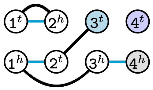
The degree of each vertex can be 0, 1 or 2 and each connected component alternates between - and -edges. As a consequence, the components of the breakpoint graph of canonical genomes can be cycles of even length or paths. An even path has one endpoint in (-telomere) and the other in (-telomere), while an odd path has either both endpoints in or both endpoints in . A vertex that is not a telomere in nor in is said to be non-telomeric. In the breakpoint graph a non-telomeric vertex has degree 2. We call -cycle a cycle of length and -path a path of length . We also denote by the number of -cycles, by the number of -paths, by the total number of cycles and by the total number of even paths. Since the number of telomeres in each genome is even (2 telomeres per linear chromosome), the total number of even paths in the breakpoint graph must be even. An example of a breakpoint graph is given in Figure 2.
2.1.2 Breakpoint distance.
For canonical genomes and the breakpoint distance, denoted by , is defined as follows [TAN-ZHE-SAN-2009]:
For and , we have . The set of common adjacencies is and the set of common telomeres is , giving . Since a common adjacency of and corresponds to a 2-cycle and a common telomere corresponds to a 0-path in , the breakpoint distance can be rewritten as
2.1.3 DCJ distance.
Given a genome, a double cut and join (DCJ) is the operation that breaks two of its adjacencies or telomeres111A broken adjacency has two open ends and a broken telomere has a single one. and rejoins the open extremities in a different way [YAN-ATT-FRI-2005]. For example, consider the chromosome and a DCJ that cuts between genes and and between genes and , creating segments , and (where the symbols represent the open ends). If we join the first with the third and the second with the fourth open end, we get , that is, the described DCJ operation is an inversion transforming into . Besides inversions, DCJ operations can represent several rearrangements, such as translocations, fissions and fusions. The DCJ distance is then the minimum number of DCJs that transform one genome into the other and can be easily computed with the help of their breakpoint graph [BER-MIX-STO-2006]:
If and , then , and (see Figure 2). Consequently, their DCJ distance is .
2.1.4 The class of distances.
Given the breakpoint graph of two canonical genomes and , for , we denote by the cumulative sums . Then the distance of and is defined to be [Chauve2018]:
It is easy to see that the distance equals the breakpoint distance and that the distance equals the DCJ distance, and that the distance decreases monotonously between these two extremes. Moreover, the distance of two genomes that form a canonical pair can easily be computed in linear time for any .
2.2 Comparing a singular and a duplicated genome
Let be a singular and be a duplicated genome over the same gene families, that is, and . The number of genes in is twice the number of genes in and we need to somehow equalize the contents of these genomes, before searching for common adjacencies and common telomeres of and or transforming one genome into the other with DCJ operations. This can be done by doubling , with a rearrangement operation mimicking a whole genome duplication: it simply consists of doubling each adjacency and each telomere of . However, when has one or more circular chromosomes, it is not possible to find a unique layout of its chromosomes after the doubling: indeed, each circular chromosome can be doubled into two identical circular chromosomes, or the two copies are concatenated to each other in a single circular chromosome. Therefore, in general the doubling of a genome results in a set of doubled genomes denoted by . Note that , where is the number of circular chromosomes in . For example, if , then with and (see Table 1). All genomes in have exactly the same multisets of adjacencies and of telomeres, therefore we can use a special notation for these multisets: and .
Each family in a duplicated genome can be -singularized by adding the index to one of its occurrences and the index to the other. A duplicated genome can be entirely singularized if each of its families is singularized. Let be the set of all possible genomes obtained by all distinct ways of -singularizing the duplicated genome . Similarly, we denote by the set of all possible genomes obtained by all distinct ways of -singularizing each doubled genome in the set .
2.2.1 The class of double distances.
The class of double distances of a singular genome and duplicated genome for is defined as follows:
Observe that for any .
2.2.2 (breakpoint) double distance.
The breakpoint double distance of and , denoted by , is equivalent to the double distance. For this case the solution can be found easily with a greedy algorithm [TAN-ZHE-SAN-2009]: each adjacency or telomere of that occurs in can be fulfilled. If an adjacency or telomere that occurs twice in also occurs in , it can be fulfilled twice in any genome from . Then,
2.2.3 (DCJ) double distance.
For the DCJ double distance, that is equivalent to the double distance, the solution space cannot be explored greedily. In fact, computing the DCJ double distance of genomes and was proven to be an NP-hard problem [TAN-ZHE-SAN-2009].
2.2.4 The complexity of double distances.
The exploration of the complexity space between the greedy linear time (breakpoint) double distance and the NP-hard (DCJ) double distance is the main motivation of this study. In the remainder of this paper we show that both and double distances can be solved in linear time.
3 Equivalence of double distance and disambiguation
A nice way of representing the solution space of the double distance is by using a modified version of the breakpoint graph [TAN-ZHE-SAN-2009].
3.1 Ambiguous breakpoint graph
Given a singular genome and a duplicated genome , their ambiguous breakpoint graph is a multigraph representing the adjacencies of any element in and a genome . The vertex set comprises, for each family in , the two pairs of paralogous vertices , and , . We can use the notation to refer to the paralogous counterpart of a vertex . For example, if , then .
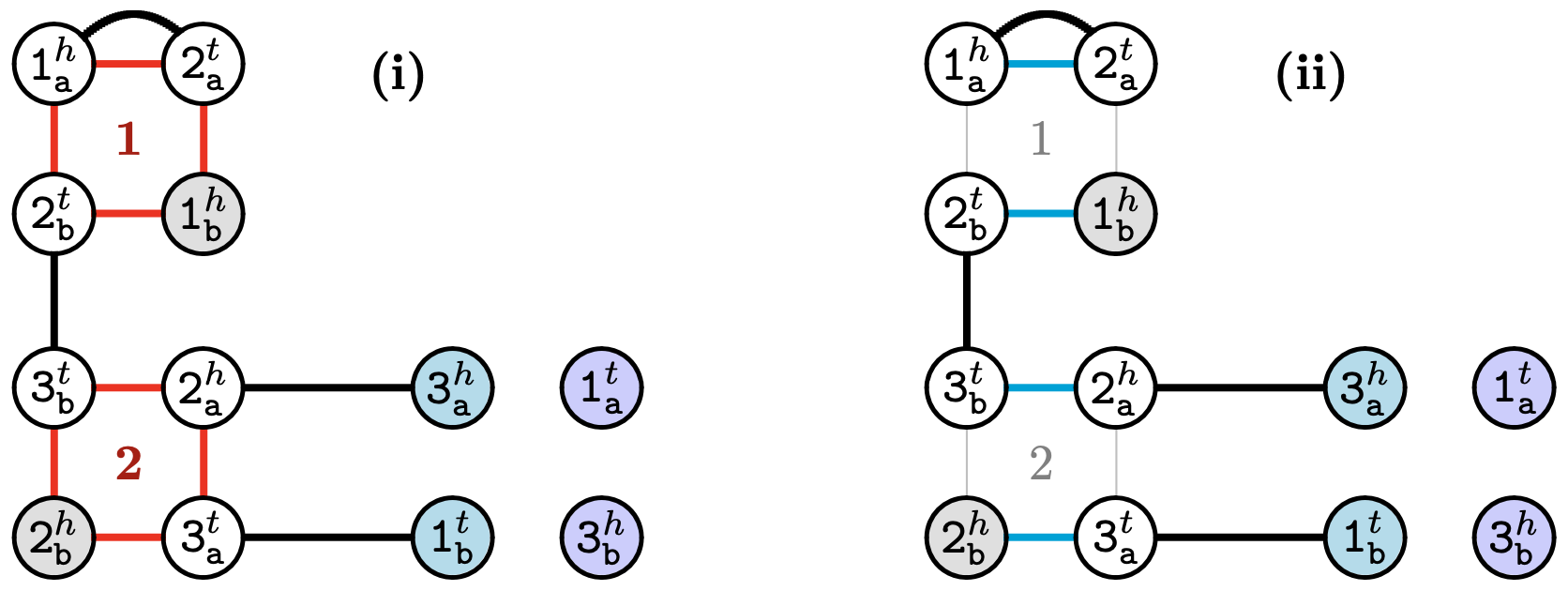
The edge set represents the adjacencies. For each adjacency in there exists one -edge in linking its two extremities. The -edges represent all adjacencies occurring in all genomes from : for each adjacency of , we have the pair of paralogous edges and the complementary pair of paralogous edges . Note that . The square of is then . The -edges in the ambiguous breakpoint graph are therefore the squares of all adjacencies in . Let be the number of squares in . Obviously we have , where is the number of linear chromosomes in . Again, we can use the notation to refer to the paralogous counterpart of an -edge . For example, if , then . An example of an ambiguous breakpoint graph is shown in Figure 3 (i).
Each linear chromosome in corresponds to four telomeres, called -telomeres, in any element of . These four vertices are not part of any square. In other words, the number of -telomeres in is . If is the number of linear chromosomes in , the number of telomeres in , also called -telomeres, is .
3.2 The class of disambiguations
Resolving a square corresponds to choosing in the ambiguous breakpoint graph either the edges from or the edges from , while the complementary pair is masked. Resolving all squares is called disambiguating the ambiguous breakpoint graph. If we number the squares of from 1 to , a solution can be represented by a tuple , where each contains the pair of paralogous edges (either or ) that are chosen (kept) in the graph for square . The graph induced by is a simple breakpoint graph, which we denote by . Figure 3 (ii) shows an example.
Given a solution , let and be, respectively, the number of cycles of length and of paths of length in . The -score of is then the sum . The minimization problem of computing the double distance of and is equivalent to finding a solution so that the -score of is maximized [TAN-ZHE-SAN-2009]. We call the latter (maximization) problem disambiguation. As already mentioned, for the double distance can be solved in linear time and for the double distance is NP-hard. Therefore the same is true, respectively, for the and the disambiguations. Conversely, if we determine the complexity of solving the disambiguation for any , this will automatically determine the complexity of solving the double distance.
An optimal solution for the disambiguation of gives its -score, denoted by . Note that, since an optimal disambiguation is also a disambiguation, although possibly not optimal, the -score of can not decrease as increases.
3.2.1 Approach for solving the disambiguation.
A player of the disambiguation is either a valid cycle whose length is at most or a valid even path whose length is at most . In order to solve the disambiguation, a natural approach is to visit and search for players. For describing how the graph can be screened, we need to introduce the following concepts. Two -edges in are incompatible when they belong to the same square and are not paralogous. A component in is valid when it does not contain any pair of incompatible edges. Note that a valid component necessarily alternates -edges and -edges. Two valid components in are either intersecting, when they share at least one vertex, or disjoint. It is obvious that any solution of is composed of disjoint valid components.
Given a solution , the switching operation of the -th element of is denoted by and replaces value by resulting in . A choice of paralogous edges resolving a given square can be fixed for any solution, meaning that can no longer be switched. In this case, is itself said to be fixed.
4 First steps to solve the disambiguation
In this section we describe a greedy linear time algorithm for the disambiguation and give some general results related to any disambiguation.
4.1 Common adjacencies and telomeres are conserved
Let be an optimal solution for disambiguation of . If a player is disjoint from any player distinct from in any other optimal solution, then must be part of all optimal solutions and is itself said to be optimal.
Lemma 1
For any disambiguation, all existing 0-paths and 2-cycles in are optimal.
Proof
While any 0-path is an isolated vertex and obviously optimal, the optimality of every 2-cycle is less obvious but still holds, as illustrated in Figure 4. ∎
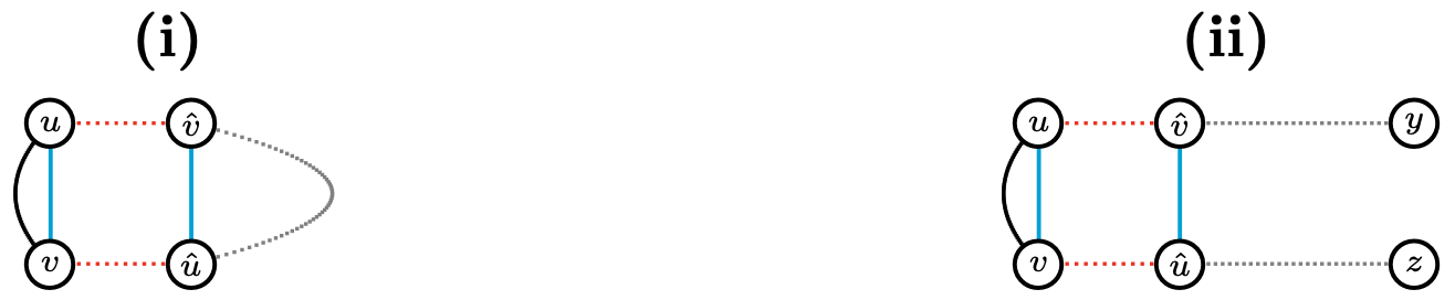
This lemma is a generalization of the (breakpoint) disambiguation and guarantees that all common adjacencies and telomeres are conserved in any double distance, including the NP-hard (DCJ) case. All 0-paths are isolated vertices that do not integrate squares, therefore they are selected independently of the choices for resolving the squares. A 2-cycle, in its turn, always includes one -edge from some square (such as square 1 in Figure 3). From now on we assume that squares that have at least one -edge in a 2-cycle are fixed so that all existing 2-cycles are induced.
4.2 Symmetric squares can be fixed arbitrarily
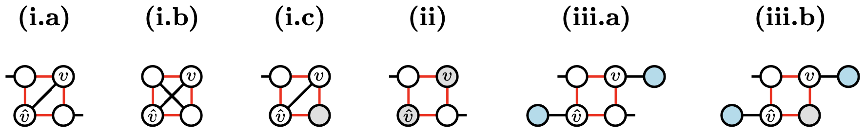
Let a symmetric square in either (i) have a -edge connecting a pair of paralogous vertices, or (ii) have -telomeres in one pair of paralogous vertices, or (iii) have -edges directly connected to -telomeres inciding in one pair of paralogous vertices, as illustrated in Figure 5. Note that, for any disambiguation, the two ways of resolving each of these squares would lead to solutions with the same score, therefore each of them can be fixed arbitrarily. From now on we assume that has no symmetric squares.
4.3 A linear time greedy algorithm for the disambiguation
Differently from 2-cycles, two valid 4-cycles can intersect with each other. But, since our graph is free of symmetric squares, two valid 2-paths cannot intersect with each other. Moreover, since a 2-path has no -edge connecting squares, a 4-cycle and a 2-path cannot intersect with each other. In this setting, it is clear that, for the disambiguation, any valid 2-path is always optimal. Furthermore, a 4-cycle that does intersect with another one is always optimal and two intersecting 4-cycles are always part of two co-optimal solutions:
Lemma 2
Any valid 4-cycle that is disjoint from a 2-cycle in is induced by an optimal solution of disambiguation.