Deep hybrid model with satellite imagery: how to combine demand modeling and computer vision for behavior analysis?

Abstract

Classical demand modeling analyzes travel behavior using only low-dimensional numeric data (i.e. sociodemographics and travel attributes) but not high-dimensional urban imagery. However, travel behavior depends on the factors represented by both numeric data and urban imagery, thus necessitating a synergetic framework to combine them. This study creates a theoretical framework of deep hybrid models with a crossing structure consisting of a mixing operator and a behavioral predictor, thus integrating the numeric and imagery data into a latent space. Empirically, this framework is applied to analyze travel mode choice using the MyDailyTravel Survey from Chicago as the numeric inputs and the satellite images as the imagery inputs. We found that deep hybrid models outperform both the traditional demand models and the recent deep learning in predicting the aggregate and disaggregate travel behavior with our supervision-as-mixing design. The latent space in deep hybrid models can be interpreted, because it reveals meaningful spatial and social patterns. The deep hybrid models can also generate new urban images that do not exist in reality and interpret them with economic theory, such as computing substitution patterns and social welfare changes. Overall, the deep hybrid models demonstrate the complementarity between the low-dimensional numeric and high-dimensional imagery data and between the traditional demand modeling and recent deep learning. It generalizes the latent classes and variables in classical hybrid demand models to a latent space, and leverages the computational power of deep learning for imagery while retaining the economic interpretability on the microeconomics foundation.

Key words: demand modeling, deep learning, satellite imagery, travel mode choice.

* To whom correspondence should be addressed. E-mail: shenhaowang@ufl.edu

1 Introduction

Demand modeling has been a theoretically rich field widely applied to various travel behavioral analyses. Researchers created the multinomial logit model to capture random utility maximization as a decision mechanism [1], the nested logit model to represent the tree structure of the alternatives [2], the mixed logit model to capture the behavioral heterogeneity in preference parameters [3], and the hybrid demand model to reveal the latent behavioral structure [4, 5, 6]. These demand models have been applied to analyze car ownership, travel mode choice, adoption of electric vehicles, and destination choice, among many other travel behaviors [7, 8, 9]. However, the existing demand models use only low-dimensional numeric data, including sociodemographic characteristics and trip attributes, while lacking the capacity to process high-dimensional unstructured data, such as urban imagery. Urban imagery has been shown to contain valuable information on built environment, socioeconomic factors, and urban mobility by recent deep learning research [10, 11, 12]. It also directly influences human decisions since people often absorb visual information before decision-making. Therefore, it seems a natural effort to extend the classical demand models to incorporate urban imagery, thus reflecting a more realistic behavioral mechanism and enriching the demand modeling tools.

To operationalize this idea, the key question is how to integrate the numeric and urban imagery data, leveraging the computational power of deep learning for urban imagery while retaining the economic interpretability of the classical demand models. On the one hand, demand models have demonstrated that travel decisions depend on travel time, travel cost, income, age, and other numeric data, which facilitates rigorous microeconomic analysis [13, 1]. The microeconomic analysis is valuable because it leverages the random utility theory to compute critical economic parameters such as social welfare and substitution patterns of alternatives [13, 14]. However, an exclusive focus on numeric data misses the tremendous opportunities in the recent big data revolution, in which unstructured data, such as urban imagery, accounts for more than 80% of data growth [15]. On the other hand, the deep learning models in the field of urban computing have used urban imagery - typically satellite or street-view images - to predict sociodemographic characteristics, achieving high predictive performance [10, 16]. However, the urban computing research exclusively focuses on using urban imagery for prediction, which lacks the rigorous microeconomic foundation and ignores the practical needs of computing elasticity, social welfare, market shares, and other important economic factors. A pure deep learning approach is like “throwing out the baby with the bath water”, since it seems implausible that travel decisions do not depend on income, age, and travel costs. Since each of the two research paradigms only partially captures behavioral realism, this dichotomy necessitates an effort to integrate them, thus successfully incorporating urban imagery into decision analysis while retaining the microeconomic foundation of the classical demand models.

This study presents a synergetic framework of the deep hybrid model (DHM), which is visually represented by a crossing structure with a vertical and a horizontal axis, as shown in Figure 1. The vertical axis represents the components in classical demand modeling, including the numeric inputs and outputs (e.g., sociodemographics, travel attributes, and behavioral outputs). The horizontal axis represents the components of deep learning, specifically an autoencoder that encodes and regenerates urban imagery. These two axes are connected through a latent space, which serves as the core to integrate the numeric data and urban imagery. This framework is named as “deep hybrid” because it resembles and extends the classical hybrid demand models [5]. It resembles the classical hybrid model because it is similar to the visual diagram (Figure 3) in [5], with our horizontal axis resembling the measurement model and our vertical axis resembling the structural model. It extends the classical hybrid demand model, because it generalizes the latent classes and variables into a latent space with higher dimensions, which is necessary for analyzing any unstructured data, including urban imagery. This framework builds upon the recent efforts in deep choice analysis [17, 18, 19], which illustrates the economic interpretability of the latent space in deep learning. However, a particular challenge is how to design an effective operator to mix the numeric data and urban imagery, thus rendering this latent space predictive and interpretable.

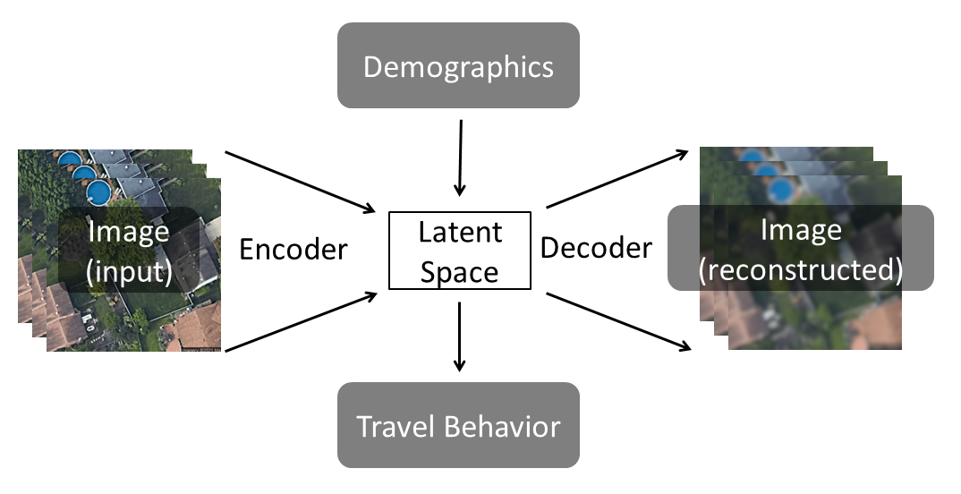
Figure 1: Diagram of the deep hybrid models

This challenge is addressed by designing a mixing operator, which encodes the numeric and imagery data into a latent space with the ideas of supervision- and concatenation-as-mixing (Section 3). The latent variables are then imported into a simple behavioral predictor, which is similar to classical demand models, thus facilitating economic interpretation. The models are empirically tested in the Chicago context, in which the MyDailyTravel Survey is used as numeric inputs and satellite imagery as the imagery inputs. Section 4 introduces data collection, local context, and experiment design. The result section (Section 5) explores three empirical questions, corresponding to our three contributions: (1) the DHM framework can effectively integrate the sociodemographics and urban imagery by outperforming both the classical demand models and deep learning (Section 5.1), (2) the latent space in DHM is spatially and socially meaningful (Section 5.2), and (3) DHM can be used to generate new urban imagery with economic interpretation, thus enabling an image-based story-telling (Section 5.3). Section 6 summarizes our findings, limitations, and broad implications.

2 Literature review

2.1 Demand modelling

Demand models have been used extensively to analyze human decision-making on travel modes [20, 18, 21], adoption of new technologies [22, 23], willingness to pay [24], and behavioral loyalty [25, 26]. The most common demand models are the class of discrete choice models (DCM) based on the theory of random utility maximization. Traditional discrete choice models use individual-specific or alternative-specific attributes as inputs, such as sociodemographics, travel time, and cost. Besides, travel decisions also depend on the psychometric features such as perceptions and attitudes, which are often modeled through latent class or variables. Although the latent variables cannot be directly measured, they can be estimated by structural equation models with the indicators collected in surveys [6]. The latent variables help to account for preference heterogeneity among the population and explain seemingly irrational behavior. To integrate the latent variables and random utility theory, hybrid choice models (HCM) are developed as a joint choice and latent variable model, and have been the state-of-the-art demand model [4, 5].

Increasingly, researchers started to enhance the power of classical demand models to account for more complex relationships in decision-making with deep learning [27, 28, 29, 30, 31, 32, 33, 34, 35]. Deep neural networks (DNNs) have shown superior performance in various applications, due to their ability to capture nonlinear relationships with flexible architecture design [36, 21]. However, DNNs are often criticized for their weak interpretability and instability of performance [37, 38]. To address these issues, some works have attempted at gradient-based methods to decipher DNN-based networks [18, 39, 40], while other studies have integrated DCM structure into the DNN architecture design. Researchers have found that the organic mixing of the two models allows for the classical economic interpretation of the choice models and reduce the sample size required for stable training of DNNs. For example, multiple works use DNNs to fit the error term from the DCM backbone [41, 42, 43], learn decision rules [44], and generate practical choice sets [45]. Researchers also used DNNs to learn latent representations from survey indicators [46], learn personal characteristics and their interactions with the alternative attributes [47], and produce embeddings for categorical variables that are typically harder to handle in traditional frameworks [48]. However, all existing studies use only numeric data, while the computational power of deep learning lies in its ability to process unstructured data, as shown by the vast number of urban imagery applications in the field of urban computing.

2.2 Computer vision in urban computing

Compared to other machine learning methods, DNN is unique due to its ability to process a variety of unstructured data (e.g., imagery, language, and graph). Although many machine learning methods can capture the nonlinear relationship between inputs and outputs, DNN’s ability to process images and natural language leads to the recent revolution in computation and big data. For example, researchers have shown that various urban images (e.g., nightlight, satellite, street view, etc.) contain rich information of urban and population characteristics. Through urban imagery, researchers can effectively learn land-use pattern classifications [49], quantify green cover [50], measure changes in the physical appearance of neighborhoods [51], and predict socioeconomic conditions [10, 11, 12, 52, 16]. In transportation, researchers have used urban imagery to monitor changing traffic flows during the pandemic [53] and predict the usage of active modes based on street view [54]. Reviews of urban imagery applications can be found in [55, 56].

However, most studies simply extract the information of tree cover, land-use features, and traffic flow from images, while overlooking the potential that urban imagery can be the direct input to analyze travel decisions. A few studies have used urban imagery to learn the perception of neighborhood safety and attitudes about neighborhoods [57, 58, 59], but we have identified no study that uses observed travel decisions as modeling outputs.

But much more important than using travel behavior as another application for computer vision, we have to design a drastically different approach from the existing urban computing research for modeling human decisions. Human decisions are much more complex than learning the built environment labels (e.g. trees, parking lots, or other land use patterns) from urban imagery, because it inevitably involves the discussions of social heterogeneity, economic implications, and human decision mechanisms (e.g., utility maximization or regret minimization). Unlike sociodemographic data, individual pixels in urban imagery do not have socioeconomic meanings, posing a unique challenge for the economic interpretation of urban imagery. Many studies have explored how to interpret the computer vision models for imagery with the latent representation [60, 61, 62], but it is unclear how to interpret urban imagery from an explicit socioeconomic perspective. To this end, we propose the DHM framework that encodes the urban imagery and the sociodemographics into a joint latent space, through which we can interpret the social aspects of urban imagery.

3 Theory

3.1 General framework of deep hybrid models

The deep hybrid model (DHM) can be represented as:

$$y_{n}=g(z_{n})=g(\mathcal{M}(x_{n},I_{n}))\\$$ (1)

in which $x_{n}$ and $I_{n}$ respectively represent the numeric and imagery inputs, $y_{n}$ represents the travel behavioral outputs. The two key components in DHM are $\mathcal{M}(x_{n},I_{n})$, which combines the numeric sociodemographics $x_{n}$ and the urban imagery $I_{n}$, and $g(z_{n})$, which predicts the output variables. In other words, the DHM framework consists of a mixing operator $\mathcal{M(\cdot)}$ and a behavioral predictor $g(\cdot)$. The behavioral predictor follows a generalized linear form: $g(z_{n})=\sigma(\beta^{\prime}z_{n})$, in which $\sigma(\cdot)$ represents the link function and $\beta^{\prime}z_{n}$ is a linear transformation of the latent variables ($z_{n}=\mathcal{M}(x_{n},I_{n})$). Note that $g(\cdot)$ is significantly simplified so that the authors could concentrate the discussion on the mixing operator; however, the $g(\cdot)$ is also flexible enough to accommodate a variety of output categories: single variable outputs, soft choice probabilities, and discrete choices.

Table 1: Design of the mixing operator.

Mixing operator	Parameter estimation	Regression analogy	Latent dim
Model 1: Only sociodemographics (SD)
$z^{(1)}_{n}=x_{n}$	NA	Linear SD	10
Model 2: Only imagery with autoencoders (IM)
$z^{(2)}_{n}=E_{\hat{\phi}}(I_{n})$	$\hat{\phi},\hat{\psi}=\underset{\phi,\psi}{\operatorname*{argmin}}\sum_{n}{||I_{n}-D_{\psi}(E_{\phi}(I_{n}))||_{2}^{2}}$	Linear IM	18,432
Model 3: Supervised sociodemographics (SSD)
$z^{(3)}_{n}=E_{\hat{\varphi}}(I_{n})$	$\hat{\varphi}=\underset{\varphi}{\operatorname*{argmin}}\sum_{n}{||x_{n}-E_{\varphi}(I_{n})||_{2}^{2}}$	Interaction SD and IM	10
Model 4: Supervised imagery with autoencoder (SIM)
$z^{(4)}_{n}=E_{\hat{\phi}}(I_{n})$	$\hat{\phi},\hat{\psi},\hat{\omega}=\underset{\phi,\psi,\omega}{\operatorname*{argmin}}\sum_{n}{||I_{n}-D_{\psi}(E_{\phi}(I_{n}))||^{2}}$ + $\lambda||F_{\omega}(E_{\phi}(I_{n}))-x_{n}||_{2}^{2}$	Interaction SD and IM	18,432
Model 5: Concatenated SD and IM (C[SD-IM])
$z^{(5)}_{n}=[z^{(1)}_{n},z^{(2)}_{n}]$	Concatenating Models 1 and 2	Linear SD + IM	10 + 18,432
Model 6: Concatenated SD, AE, SSD, and SAE (C[SD-IM-SSD-SIM])
$z^{(6)}_{n}=[z^{(1)}_{n},z^{(2)}_{n},z^{(3)}_{n},z^{(4)}_{n}]$	Concatenating Models 1, 2, 3, and 4	Linear and Interaction SD + IM	10*2 + 18,432*2

The design of the mixing operator $\mathcal{M}(x_{n},I_{n})$ is the main focus, with six specific examples summarized in Table 1. The first two models are the benchmarks that use only sociodemographics and only urban imagery as inputs. In Table 1, the first column specifies how we obtain the latent space $z^{(i)}$ in each model $i$; the second column specifies how the mixing operator is trained. For example, in Model 2, $\hat{\phi},\hat{\psi}=\underset{\phi,\psi}{\operatorname*{argmin}}\sum_{n}{||I_{n}-D_{\psi}(E_{\phi}(I_{n}))||_{2}^{2}}$ means that $\hat{\phi},\hat{\psi}$ are the parameters to be estimated for encoder $E_{\phi}(\cdot)$ and decoder $D_{\psi}(\cdot)$ of the autoencoder, and $\sum_{n}{||I_{n}-D_{\psi}(E_{\phi}(I_{n}))||_{2}^{2}}$ is the reconstruction loss to be minimized. The third column uses the regression terminology to explain the types of relatinoships incorporated in each model. The last column specifies the dimension of $z^{(i)}$. Model 1 (SD) simply uses the $x_{n}$ without including any imagery information. Model 2 (IM) uses the latent neurons from only urban imagery, which is trained through an autoencoder ($E_{\phi}$ and $D_{\psi}$) without including any sociodemographic information. The autoencoder parameters $\phi$ and $\psi$ are trained by minimizing the mean squared error between original image $I_{n}$ and the reconstructed $D_{\psi}(E_{\phi}(I_{n}))$. Model 3 (SSD) and 4 (SIM) adopt the idea of “supervision-as-mixing”, which will be discussed in details in Section 3.2. Simply put, in both models, images are used to predict sociodemographics with the intermediate neurons absorbing information from both data sources. Model 3 directly predicts sociodemographics, while Model 4 combines image reconstruction and sociodemographics prediction via multi-task learning through a shared latent space. Intuitively, Models 3 and 4 create interactions between sociodemographics and urban imagery, similar to the interaction terms in regressions. Models 5 and 6 mix the two data structures by concatenating the latent spaces from Models 1-4. Concatenation is the standard way of combining information, which also facilitates our analysis regarding the sources of information. The dimensions of the latent space in the six models are drastically different. As shown in Table 1, Models 1 and 3 use very low-dimensional latent space to represent sociodemographics, while all other models’ latent spaces are relatively high dimensional because of the necessity to encode urban imagery. This high dimensionality necessitates the adoption of LASSO regressions in our behavioral predictor $g(\cdot)$.

This DHM framework is partially inspired by the state-of-the-art hybrid demand models [4, 5]. In hybrid demand models, a structural component describes how the sociodemographic variables relate to travel behavior, and a measurement model describes the relationship between observed variables and latent variables. Our DHMs have a similar structure, but we design the latent space to incorporate urban imagery and generalizes the low-dimensional latent variables/classes to a latent space with higher dimensions.

3.2 Mixing operator: supervision and concatenation as mixing

The main approach is named as supervision-as-mixing, because we use the hidden neurons in supervised learning to mix the numeric and imagery data. In Model 3, the urban imagery $I$ is used in a neural network to predict the numeric inputs $x$, so the hidden neurons can represent a mixture of the sociodemographics and the imagery data. As shown on the left in Figure 2, Model 3 uses a ResNeXt architecture [63] to predict sociodemographics $x$ from urban imagery, and the latent space is the predicted sociodemographics $z^{(3)}_{n}=\hat{x}_{n}=E_{\hat{\varphi}}(I_{n})$. This ResNeXt architecture is an extension of the standard ResNet architecture[64], and is used throughout the study as the encoders and decoders in Models 3-6. Model 4, shown on the right in Figure 2, uses a supervised autoencoder, which uses multi-task learning to combine an autoencoder with the supervision of sociodemographics. Model 4’s latent variable $z^{(4)}_{n}$ is passed through the decoder network $D_{\psi}(z_{n})$ for the reconstructed image, and through another smaller network $F_{\omega}(z_{n})$ for the predicted sociodemographics. This multi-task learning structure enables the latent space to represent and mix both data sources. The loss function for the supervised autoencoder is

$$\underset{\phi,\psi,w}{\operatorname*{argmin}}\sum_{n}{||I_{n}-D_{\psi}(E_{\phi}(I_{n}))||^{2}+\lambda||F_{\omega}(E_{\phi}(I_{n}))-x_{n}||_{2}^{2}}$$ (2)

in which the first term represents the image reconstruction loss, the second term represents the prediction loss from sociodemographics, and the $\lambda$ is the mixing hyperparameter that adjusts the tradeoff between the prediction loss and the image reconstruction loss. When $\lambda\rightarrow 0$, the latent space contains only imagery information. When $\lambda\rightarrow+\infty$, the latent space contains only sociodemographic information. Hence this $\lambda$ hyperparameter adjusts the information mixing ratio between the two data structures.

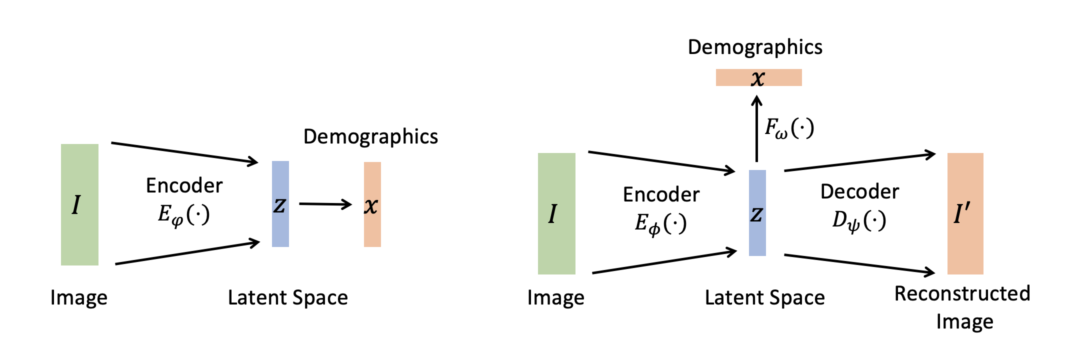
Figure 2: Supervision as mixing. Left figure (Model 3): urban imagery is used to predict sociodemographics with the hidden neurons used as $z$; right figure (Model 4): urban imagery is used in an autoencoder with supervised training for sociodemographics $x$, and the hidden neurons are used as $z$

Supervision-as-mixing in Model 4 not only mixes two data structures through multi-task learning, but also enhances the stability and interpretability of the latent space. Through autoencoder, the urban imagery can be condensed into a latent space. With the supervision of sociodemographics, this latent space can be significantly stablized, because Equation 2 can also be viewed as regularization [65]. Both multi-task learning and regularization help to constrain the latent space and thus promote stability [66, 67].

To mix the two data structures, a simple concatenation is a relatively straightforward approach. The simple concatenation has neither the benefits of generating sociodemographics information, nor stabilizing latent space as supervision-as-mixing. However, its simplicity allows us to trace the predictive power of the numeric and the urban imagery data. For example, in Model 5, the sociodemogrpahics $x_{n}$ from Model 1 is concatenated with the latent neurons $E_{\hat{\phi}}(I_{n})$ from Model 2 to create a joint latent space. With LASSO regularization, we could identify the non-zero coefficients from the concatenated space, which could inform how the sociodemographics and urban imagery independently contribute to behavioral prediction.

3.3 Behavioral predictor

The behavioral predictor $g(z)$ is designed as a generalized linear regression:

$$\hat{y}=g(z)=\sigma(\beta^{\prime}z)$$ (3)

This form is intentionally designed with simplicity so that we could focus on discussing the mixing operator. But Equation 3 is also flexible enough to accommodate various output variables. Three categories of output variables are modeled: (1) aggregate travel mode shares as individual outputs, (2) aggregate travel mode shares as a joint output, and (3) individual travel mode choices. A general form of training the behavioral predictor is:

$$\underset{\beta}{\operatorname*{argmin}}\ L(y_{n},\sigma(\beta^{\prime}z_{n}))+\theta||\beta||_{p}$$ (4)

in which $L(y_{n},\sigma(\beta^{\prime}z_{n}))$ represents the loss function (e.g. mean squared error or negative log likelihood), $\beta$ represents the parameters, $\theta$ is the sparsity hyperparameter to control the sparsity of $\beta$. In all three examples, the sparsity hyperparameter $\theta$ serves as the weight for L1 (LASSO) regularization to address overfitting and to identify the relevant input variables. The three outputs are specified in the following three subsections.

3.3.1 Aggregate travel mode shares as separate outputs

The first example is relatively straightforward: since the outcome $y_{n}$ is a continuous scalar to represent the aggregate travel mode shares, the link function $\sigma$ is specified as an identity mapping:

$$\sigma(\beta^{\prime}z_{n})=\beta^{\prime}z_{n}$$ (5)

The mean squared error in linear regression is used as the loss for model fitting.

3.3.2 Aggregate travel mode shares as a joint output

The second example uses the aggregate travel mode shares as a joint output of the model. Since the joint mode shares should add up to one, a softmax function is specified as the link function to ensure the validity of this constraint. Using the linear transformation on $\beta^{\prime}z_{n}$, we could represent the output mode shares as:

$$\begin{split}P_{nk}=\frac{e^{V_{nk}}}{\sum_{j}e^{V_{nj}}}=\frac{e^{\beta^{\prime}_{k}z_{n}}}{\sum_{j}e^{\beta^{\prime}_{j}z_{n}}}\end{split}$$ (6)

in which $P_{nk}$ represents the market shares of mode $k$ in region $n$. Since the market share of the travel modes of a region follows a probability distribution, Kullback-Leibler (KL) loss is used to specify the general loss in Equation 4:

$$L_{KL}=\frac{1}{N}\sum_{n=1}^{N}{\sum_{k=1}^{K}{P_{nk}(\ln{P_{nk}}-\ln{\hat{P}_{nk}})}}$$ (7)

3.3.3 Disaggregate travel mode choice

The third example uses individual travel mode choice as the model outputs. The choice probabilities of trip $n$ being taken using alternative $k$ can be specified as

$$P_{nk}=\frac{e^{V_{nk}}}{\sum_{j}e^{V_{nj}}}$$ (8)

where $P_{nk}$ is the probability of trip $n$ taken with alternative $k$, $V_{nk}$ is the utility of alternative $k$ for trip $n$. Since the disaggregate travel mode choice involves origin-destination pairs, the alternatives’ attributes for each OD pair concatenate the origin $o_{n}$ and destination $d_{n}$: $z_{n}=[z_{o_{n}},z_{d_{n}}]$. Similar to the aggregate travel mode analysis, the utility function takes a simple linear form as $V_{nk}=\beta^{{}^{\prime}}_{k}z_{n}$. However, since discrete choice models have unique data structures in the input variables, which consist of individual-specific and alternative-specific variables, the detailed specification is slightly different from the aggregate travel mode analysis (Appendix I). Let $y_{nk}$ represent the observed mode ($y_{nk}=1$ if mode $k$ is used for trip $n$, and $y_{nk}=0$ otherwise), and $N$ is the total number of trips. Cross entropy loss can be used to substantiate the training loss in Equation 4:

$$L_{ce}=\frac{1}{N}\sum_{t=1}^{N}{\sum_{k=1}^{K}{-y_{nk}\ln{P_{nk}}}}$$ (9)

3.4 Two-step training

In short, the training of DHMs takes two steps - training the mixing operator and then the behavioral predictor - as summarized in Figure 3. Using the SIM as an example, on stage I, we train the supervised autoencoder only, which consists of the encoder $E_{\phi}(I)$, decoder $D_{\psi}(z)$, and the sociodemographics predictor $F_{\omega}(z)$. Each input image is encoded into a latent variable $z$, which then passes through $F_{\omega}(z)$ and $D_{\psi}(z)$ to reconstruct sociodemographics and images. On stage II, the parameters of the supervised autoencoder are fixed, so only the behavioral predictor $g(z)$ is trained. In testing, an input image is encoded into a latent variable $z$, which then reconstructs socio-demographics and an image through $F_{\omega}(z)$ and $D_{\psi}(z)$, and predicts travel behaviors through $g(z)$.

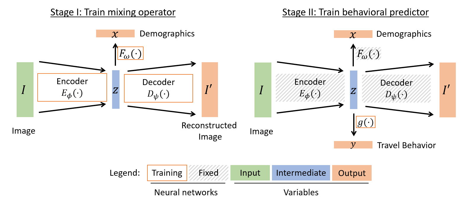
Figure 3: Two-step training

3.5 Economic interpretation

Although DHMs leverage the power of deep learning, they are interpretable with economic information in the aggregate and disaggregate travel mode analysis. This economic interpretability is enabled by the softmax activation function, which is thoroughly discussed in a recent work [18]. Here we provide the formula for computing market shares, substitution patterns of alternatives, social welfare, and choice probability derivatives with an emphasis on the innovation of using latent variable $z$ to connect images, sociodemographics, and travel behaviors. Specifically, the market share of alternative $k$ can be computed as

$$s_{k}=\sum_{n}{P}_{nk}=\sum_{n}\frac{e^{V_{nk}}}{\sum_{j}e^{V_{nj}}}$$ (10)

Social welfare of individual $n$ takes the standard logsum formula:

$$\frac{1}{\alpha_{n}}\log(\sum_{j}e^{{V}_{nj}})$$ (11)

where $\alpha_{n}$ measures the marginal utility of income that translates social welfare into dollar values. The substitution pattern for two alternatives $j$ and $k$ is defined as the ratio of their choice probabilities:

$$\frac{P_{nj}}{P_{nk}}=\frac{e^{V_{nj}}/\sum_{k^{\prime}}e^{V_{nk^{\prime}}}}{e^{V_{nk}}/\sum_{k^{\prime}}e^{V_{nk^{\prime}}}}=e^{V_{nj}-V_{nk}}$$ (12)

Although the three equations above appear similar to those in the standard demand models, they implicitly incorporate satellite imagery to compute the utility value $V_{nk}$ through the latent variable $z$. It is because $V_{nk}=\beta^{\prime}_{k}z_{n}$, in which $z_{n}$ contains imagery $I_{n}$ as an input, as shown in Table 1. In fact, among the six models in Table 1, five of them (Model 2-6) embed both satellite images and sociodemographic variables into the latent variable $z_{n}$. As a result, whenever we provide a new value $\tilde{z}$ in the latent space, it can be used to visualize a satellite imagery through the decoder as $\tilde{I}=D_{\psi}(\tilde{z})$, and meanwhile, compute the utility $V_{nk}(\tilde{z})$, market shares, social welfare, and substitution patterns with Equations 10, 11, and 12.

Using the DHMs, we could further compute a directional gradient of choice probabilities regarding the latent variable $z$, which resembles but also differs from the marginal effects $\beta$ in the classical demand modeling. The formula of the directional gradient is

$$\nabla_{u}P_{nk}({z})={u}\cdot\nabla P_{nk}({z})$$ (13)

where $\nabla P_{nk}({z})$ represents the gradient of choice probability regarding the latent variable $z$, and ${u}$ represents a direction to move in the latent space. This directional gradient resembles the marginal effects in the classical demand models because it can be used to compute the sensitivity of choice probabilities with respect to the latent variable $z$, which is a common practice in the interpretation of the classical latent variable models. But since DHMs connect $z$ and urban imagery $I$, this directional gradient can also describe the sensitivity of choice probabilities with respect to a satellite image $I$ that is corresponding to the latent variable $z$. It is feasible to calculate the sensitivity of choice probabilities regarding satellite images simply because autoencoder connects the latent variable $z$ and satellite images in the DHM.

However, this metric for the sensitivity of choice probabilities regarding images needs to be limited to a certain direction $u$ to generate images of high quality. The direction can be defined as ${u}={z_{2}}-{z_{1}}=E(I_{2})-E(I_{1})$ by using two existing images $I_{1}$ and $I_{2}$. This one-directional movement can be extended to a multi-directional movement by linearly combining multiple $u$’s: ${u}=a_{1}{u_{1}}+a_{2}{u_{2}}$, where $u$ takes into account two directions ${u_{1}}$ and ${u_{2}}$. In our empirical analysis, we will demonstrate the directional sensitivity of choice probabilities regarding satellite images by discretizing the latent space. For example, we can create a directional vector $u=z_{2}-z_{1}$ to define the directional movement, and compute the choice probabilities and satellite images using a new latent variable $\tilde{z}={z_{1}}+a{u}={z_{1}}+a({z_{2}}-{z_{1}})$, in which $a\in\{0.0,0.2,0.4,0.6,0.8,1.0,1.2,1.4,1.6\}$. With this approach, we can visualize a new satellite image $\tilde{I}$ through the decoder as $\tilde{I}=D_{\psi}(\tilde{z})$ and compute the choice probabilities through the behavioral predictor as $g(\tilde{z})$. We can also compute market shares, social welfare, and substitution patterns by applying $V_{nk}(\tilde{z})$ to Equations 10, 11, and 12. The empirical results are demonstrated in Section 5.3.

4 Experiment design

4.1 Data

The experiments use multiple data sources from Chicago, including satellite images from Google API, socio-demographics from the census, and individual travel behavior from MyDailyTravel Survey conducted in 2018-2019 [68]. After data preprocessing, The dataset has $1,571$ such census tracts with a total of $80$k observed trips.

The satellite images have a standard 224 $\times$ 224 size, with samples shown in Figure 4. To represent the census tracts, the same number of satellite image patches were sampled from all the census tracts, which are then linearly combined in the latent space of the DHM as the representative imagery features. The sociodemographics are obtained from the American Community Survey (ACS), which includes total population, age groups, racial composition, education, economic status, and some travel information (e.g. commuting time). The satellite images and ACS data are used in the aggregate behavioral analysis.

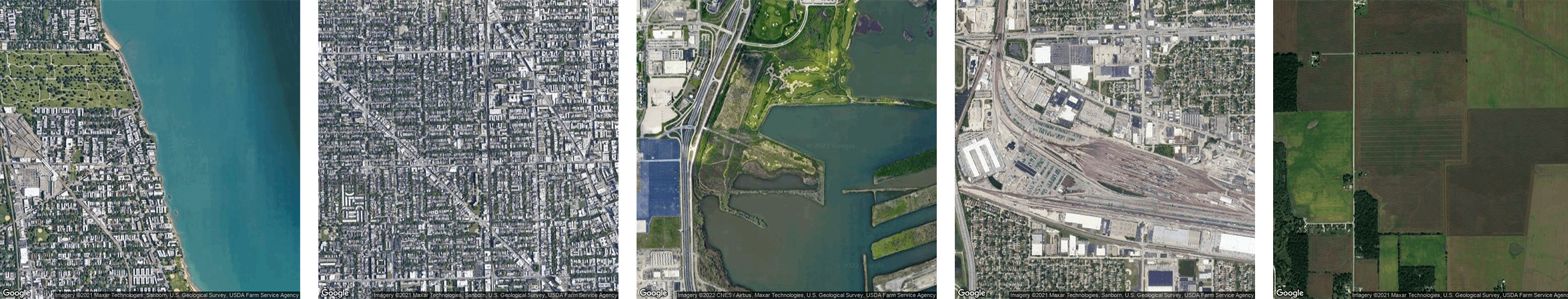
Figure 4: Samples of satellite images

The MyDailyTravel survey provides individual sociodemographics and trip-level attributes for the disaggregate analysis. It contains $42$ variables, including time of the trip (morning/after), trip distance, home-based trips, trip purposes, perceived time importance, age, disability, and education, among many other travel and social factors. The initial travel modes have more than ten categories, but they are aggregated into auto, active (walk+bike), public transit, and others, thus creating a relatively balanced choice set.

4.2 Specifying the mixing operator

The architecture, normalization, optimizer, and hyperparameters of the mixing operator are explored for successful data mixing. The architectures in the encoder-decoder are ResNeXt with the same specifications as the setup in [63]. The resulting latent space dimension is $18,432$. Three feed-forward layers with ReLU activation project the latent space $z$ to the sociodemographics $x$ in supervised autoencoders. Data is preprocessed with min-max normalization. The optimizer is stochastic gradient descent (SGD), with the learning rate and weight decay parameters selected as $0.001$ and $0.0001$ to ensure convergence and mitigate overfitting.

In the design of the mixing operator, an important hyperparameter is the mixing hyperparameter $\lambda$, which balances the reconstruction loss $L_{r}$ and the supervision loss $L_{s}$, thus controlling the extent to which the imagery and numeric data are mixed. The value of $\lambda=10$ indicates that the two losses are of the same magnitude, whereas $\lambda=0$ implies only imagery information without sociodemographics. The hyperparameter values are tested in a logarithmic scale ($\lambda=0,1,10,100,1,000,10,000$) to evaluate the impacts of the mixing hyperparameter on model performance.

Since each census tract has multiple images, we average the image representations linearly to create a representative vector for a census tract in the latent space. Previous studies have shown that the encoded latent space can be interpolated by the convex combinations of latent variables from two different images [69, 70]. Therefore, we average the latent variables of the images to represent census tracts: $z_{s}=\frac{1}{I_{s}}\sum_{i=1}^{I_{s}}{z_{i}}$, where $z_{s},z_{i}$ is the latent representation of a region $s$ and image $i$, and $I_{s}$ is the number of images corresponding to region $s$.

4.3 Specifying the behavioral predictors

With the latent representation $z_{s}$ as the input, three groups of the travel behaviors are used as the outputs of the behavioral predictors: aggregate travel mode shares as separate outputs and a joint output, and the disaggregate individual travel mode choices. The mode shares of each census tract are calculated as the average of the trips that originate from the census tract. For aggregate travel mode share as separate outputs, LASSO regularization is used to isolate the effect of the mixing operator and stabilize the behavioral predictor. LASSO regression imposes sparsity and helps to isolate the effect of sociodemographics from urban imagery when they are concatenated. The $R^{2}$ is calculated on the auto, active, and public transit separately for model evaluation. For the disaggregate MNL model, the classical cross-entropy loss and accuracy rates are used.

In the behavioral predictors, an important hyperparameter is the sparsity hyperparameter $\theta$, because it controls model sparsity and enhances generalizability. The sparsity hyperparameter $\theta$ and the mixing hyperparameter $\lambda$ are searched together in a prespecified space. Both hyperparameters $\lambda$ and $\theta$ are critical for the success of the DHM, so their effects are examined closely in the following result section.

5 Results

In this section, we first demonstrate the complementarity of sociodemographics and urban imagery through the DHM framework, as shown by the DHMs with supervision-as-mixing outperforming the demand models, deep learning, and the simple concatenation of the two data structures. Second, we discuss the effect of the mixing ($\lambda$) and sparsity ($\theta$) hyperparameter on model performance. Next, we show the rich social and spatial contents encoded in the latent space, and how to use the latent space to generate new urban imagery. Finally, we present the economic interpretation of urban imagery, thus presenting an image-based story-telling that was not explored in the classical demand modelling framework or the current computer vision literature.

5.1 Model performance

Table 2 summarizes the results of the six models in three travel behavior tasks with six columns and three panels. Panels 1 and 2 present the aggregate analysis of travel mode choice using linear regressions separately on each travel mode and MNL for training the travel modes jointly with KL-divergence loss. Panel 3 presents the disaggregate analysis of individual mode choice. Columns 1 and 2 represent the two benchmark models (Models 1-2) using only sociodemographics and urban imagery, and Columns 3-6 represent the DHMs (Models 3-6) with the design of concatenation- and supervision-as-mixing. The first row in each panel shows the number of variables in each behavioral predictor. Panels 1 and 2 represent the aggregate models, with 10 sociodemographic variables and a latent variable of length 18432 representing urban imagery for each census tract. Panel 3 represents the individual choice model. In addition to census tract level information, each model is appended with 42 trip/individual attributes. Table 2 covers three tasks and six models, each with a different optimal $\lambda$ and $\theta$. To make the comparison fair, every entry in Table 2 represents the training/testing performance after the best $\lambda$ and $\theta$ are selected by the highest performance in the testing set. The effects of $\lambda$ and $\theta$ on model performance are investigated in later sections. In the aggregate cases where the latent space has more dimensions than the sample size, we performed a 5-fold cross-validation to evaluate the model performance. The results are in Table A1 in the Appendix.

Table 2: Model performance

	1	2	3	4	5	6
	SD	IM	SSD	SIM	C[SD-IM]	C[SD-IM-SSD-SIM]
Panel 1: Aggregate Mode Choice as Separate Outputs - Linear Regression
Input Dim	10	18432	10	18432	10+18432	10*2+18432*2
Auto ($R^{2}$)	0.44/0.50	0.72/0.63	0.59/0.64	0.73/0.73	0.73/0.65	0.69/0.71
Active ($R^{2}$)	0.35/0.47	0.60/0.50	0.47/0.52	0.56/0.56	0.61/0.52	0.55/0.56
PT ($R^{2}$)	0.39/0.29	0.63/0.44	0.47/0.52	0.58/0.54	0.65/0.47	0.60/0.54
Panel 2: Aggregate Mode Choice as a Joint Output - Multinomial Regression
Input Dim	10	18432	10	18432	10+18432	10*2+18432*2
KL Loss	0.17/0.15	0.14/0.12	0.15/0.13	0.09/0.10	0.13/0.12	0.10/0.10
Auto ($R^{2}$)	0.41/0.45	0.58/0.63	0.52/0.56	0.80/0.74	0.61/0.63	0.74/0.58
Active ($R^{2}$)	0.34/0.44	0.49/0.50	0.41/0.44	0.76/0.61	0.51/0.52	0.67/0.72
PT ($R^{2}$)	0.34/0.23	0.46/0.47	0.42/0.46	0.78/0.52	0.52/0.46	0.66/0.50
Panel 3: Disaggregate Mode Choice - Discrete Choice Analysis
Input Dim	42+10*2	42+18432*2	42+10*2	42+18432*2	42+10*2+18432*2	42+10*4+18432*4
CE Loss	0.423/0.422	0.422/0.422	0.408/0.407	0.396/0.410	0.424/0.408	0.379/0.403
Accuracy	0.856/0.857	0.853/0.853	0.860/0.861	0.861/0.857	0.851/0.853	0.870/0.864
Note: each entry is represented as training/testing performance.

First of all, both the numeric and urban imagery data contain valuable information for travel behavior, although urban imagery provides more information for the aggregate analysis than the disaggregate one. Both Models 1 and 2 can achieve a $R^{2}$ substantially higher than zero, indicating that the numeric and imagery data can provide valuable information for travel behavioral analysis independently. In Panel 1, the testing $R^{2}$ of urban imagery is 0.63, 0.50, and 0.44 for automobiles, active travel modes, and public transit in Column 1, as opposed to 0.50, 0.47, and 0.29 in Column 2, indicating that urban imagery provides more information than the numeric data in the aggregate analysis. This finding holds the same in Panel 2, while it changes in Panel 3, since unsurprisingly, the individual characteristics matter more than the aggregate satellite imagery in the prediction of individual travel behaviors.

The images and the numeric data are complementary, as shown by the DHMs (Models 3-6) outperforming the two benchmarks (Models 1-2) in all the experiments. In the aggregate case, Model 3 outperforms Model 1, indicating the effectiveness of supervision-as-mixing in combining sociodemographics and urban imagery even when the dimension of the latent space is low. Model 3 has a similar performance as Model 2, where the magnitude of $R^{2}$ improvement ranges from 5% (for the active mode) to around 20% (for the PT mode) compared to Model 1. On the other hand, Model 4 achieves the best performance because the latent space is large enough to encode the imagery information. Model 4 improves the $R^{2}$ by 2% to 18% compared to Model 3. In the disaggregate case, the urban imagery improves the predictive performance moderately because travelers’ sociodemographics and travel features appear more important. Models 3 and 4 yield about 4% improvement in KL loss and 0.5% improvement in accuracy in comparison to Models 1 and 2, which are their unsupervised counterparts. This improvement is evident but of a moderate magnitude, particularly in comparison to the significant improvement in the aggregate behavioral analysis (Panels 1 and 2).

Supervision-as-mixing is much more effective than the simple concatenation in integrating the numeric and imagery data, which can be shown by comparing Models 4, 5, and 6. Model 4 outperforms Model 5 by 4% to 9% regarding $R^{2}$ in the aggregate cases and around 0.5% regarding the CE loss and accuracy in the disaggregate cases, indicating that the supervision-as-mixing in Model 4 is more effective than concatenation in Model 5. Meanwhile, Model 6 often performs similarly to Model 4, indicating that the extra variables in Model 6 from the simple concatenation can not effectively improve the performance of the supervision-as-mixing design. In addition, the high dimensionality in the latent space is critical for the success of supervision-as-mixing. When the dimensionality is low (i.e., Model 1), the DHM (Model 3) has only limited improvement even after encoding the urban imagery. When the dimensionality is high, the DHM (i.e., Model 4) has much more flexibility in information encoding and thus achieves higher performance.

Besides comparing performance, the complementarity of the two data structures can also be observed by the number of non-zero coefficients in Model 5, which approximate the informativeness of the two data structures in predicting travel behavior. The non-zero coefficients are computed by adjusting the sparsity hyperparameter $\theta$ in Model 5, as shown in Figure 5. When the sparsity hyperparameter $\theta$ increases, the number of the nonzero coefficients from both the numeric and the imagery data decreases. When the sparsity hyperparameter $\theta=0$, the number of non-zero coefficients from images is around 2,000 times larger than that from the sociodemographic variables (10). But it drops to zero much more quickly than sociodemographics as $\theta$ increases. At the optimal point $\theta=2e-4$, the number of nonzero coefficients from images is only around 50 times larger than that of sociodemographic variables. The optimal non-zero coefficients consist of six sociodemographic variables (60%) and 335 imagery variables (2%), demonstrating the independent contribution from and the complementarity between the sociodemographic and imagery information.

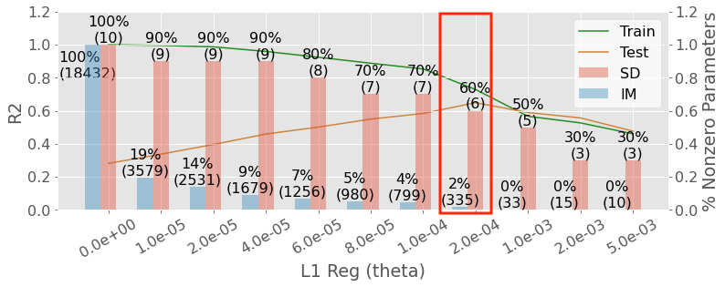
Figure 5: Data complementarity demonstrated by the non-zero coefficients from sociodemographics and urban imagery

5.1.1 Importance of the mixing hyperparameter $\lambda$

The mixing hyperparameter $\lambda$ controls the balance between reconstruction and sociodemographics prediction in autoencoders, and thus indirectly affects the predictive performance of behavioral predictors. Table 3 shows the predictive performance under different $\lambda$ values. To isolate the effect of $\lambda$, we present the results with $\theta$ tuned to the optimal value for each $\lambda$. That is, the results in Table 3 are produced with different $\theta$ values.

The improvement of performance can be quite significant by optimizing $\lambda$. Since $\lambda$=0 represents an autoencoder without sociodemographic information, the non-zero $\lambda$ values in Table 3 imply the success of mixing the two data structures by balancing the mixing hyperparameter $\lambda$. For example, the $R^{2}$ of predicting the aggregate automobile usage is 0.647 when $\lambda=1$, while the optimal $R^{2}=0.722$, which improves the performance by 11.6%. This significant improvement is quite consistent across the models and tasks, although the improvement in the disaggregate analysis appears less significant. The optimal CE Loss equals 0.409, improving upon the baseline performance (0.423) by 3.4%. The effect of $\lambda$ is less in disaggregate models because urban imagery naturally represents aggregate information that is not sufficiently specific to capture individual heterogeneity. Urban imagery information casts less influence on model performance as it is only a supplementary data source to the individual and trip-level attributes in the disaggregate choice model.

The magnitude of the optimal $\lambda$ varies with the tasks. In the aggregate model, more regularization is desired, because the sociodemographic information enters the behavioral model only through the latent space. In order for the latent space to incorporate information from both imagery and sociodemographics, a large regularization is needed. Meanwhile, in the disaggregate model, individual-specific sodiodemographics and trip-level attributes are available, making the aggregate sociodemographics redundant. Therefore, pure imagery information, which does not exist in the individual and trip-level attributes, is desired. Hence a smaller $\lambda$ performs better.

Table 3: Effects of the mixing hyperparameter $\lambda$ in Model 4

The mixing hyperparameter $\lambda$	$1e^{-1}$	$1e^{0}$	$1e^{+1}$	$1e^{+2}$	$1e^{+3}$
Panel 1: Aggregate Mode Choice - Linear Regression
Auto ($R^{2}$) ($\theta=8e^{-4}$)	0.476/0.572	0.566/0.647	0.679/0.669	0.701/0.720	0.707/0.705
Active ($R^{2}$) ($\theta=6e^{-4}$)	0.384/0.458	0.429/0.519	0.528/0.532	0.560/0.532	0.563/0.562
PT ($R^{2}$) ($\theta=4e^{-4}$)	0.362/0.397	0.450/0.421	0.564/0.480	0.579/0.544	0.599/0.539
Panel 2: Aggregate Mode Choice - Multinomial Regression ($\theta$=$1e^{0}$)
KL Loss	0.152/0.124	0.140/0.115	0.093/0.110	0.087/0.106	0.086/0.101
Auto ($R^{2}$)	0.523/0.606	0.588/0.641	0.778/0.708	0.800/0.747	0.808/0.746
Active ($R^{2}$)	0.433/0.493	0.474/0.540	0.716/0.516	0.759/0.527	0.758/0.611
PT ($R^{2}$)	0.404/0.431	0.489/0.449	0.750/0.488	0.793/0.534	0.777/0.523
Panel 3: Disaggregate Mode Choice ($\theta$=$1e^{-3}$)
CE Loss	0.451/0.448	0.409/0.409	0.409/0.421	0.414/0.423	0.410/0.423
Accuracy	0.842/0.843	0.858/0.857	0.856/0.852	0.854/0.852	0.855/0.851

The mixing hyperparameter $\lambda$ affects the performances in downstream behavioral predictors by controlling the degree of information mix in the latent space. The degree of information mix can be understood by the tradeoff between retaining the richness in image reconstruction and encoding sociodemographic information. The reconstruction MSE and sociodemographics prediction error with respect to changing $\lambda$ are shown in Figure 6. Reconstructions MSE refers to the normalized intensity of image pixels in the RGB channels. The sociodemographics are min-max normalized so that all variables are between $[0,1]$ for easy training and comparison. With increasing $\lambda$, the latent space contains more information relating to the sociodemographics, and retains less for image reconstruction, evidenced by increasing reconstruction error and decreasing prediction error. To provide a more intuitive view of the reconstruction quality, Figure A1 in the Appendix shows two sample image reconstructions with respect to changing $\lambda$. A $\lambda$ value larger than 1 will make image reconstruction quality suffer. While $\lambda$ less than or equal to 1 will make the sociodemographic prediction error higher. While all errors (even with a small $\lambda$) are less than 0.06, $\lambda$ does not affect the sociodemographic variables evenly. For example, population density, age, average travel time to work, and income have smaller errors and are less affected by the value of $\lambda$. However, variables related to race and education have large errors and are more sensitive to changes in $\lambda$.

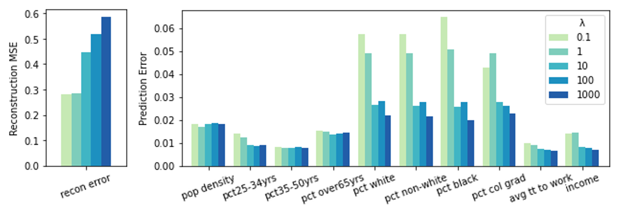
Figure 6: Image reconstruction and sociodemographics prediction error with varying $\lambda$

The choice of $\lambda$ presents a challenge and calls for case-by-case treatment. If the goal of the model is not to synthesize new images, the loss in image details should not matter as information relevant to travel behavior is encoded in the latent space. However, if we want to generate high-quality images, we can always use a smaller $\lambda$ value with some sacrifice in the predictionaccuracy of travel behavior.

5.1.2 Effect of the sparsity hyperparameter $\theta$

In addition to the mixing hyperparameter $\lambda$, the choice of the sparsity hyperparameter $\theta$ is also key to higher model performance. The importance of $\theta$ can be observed by Table 4, in which a non-zero $\theta$ value is always necessary in all our models and tasks to achieve the highest testing performance. Unlike $\lambda$, the explored range of $\theta$ values heavily depends on the type of behavioral predictor. For example, to observe around 5% performance difference, $\theta$ testing range for LASSO regression is an arithmetic sequence (from $2e^{-4}$ to $1e^{-3}$), while for MNL models is a geometric sequence (from $1e^{-1}$ to $1e^{+3}$, and from $1e^{-5}$ to $1e^{-1}$). Within the same type of model, the effect of $\theta$ does not heavily depend on the tasks. For example, the LASSO regression $R^{2}$ differences for auto, public transit, and active modes (Panels 1.1 - 1.3) are all around 0.05 (0.66 to 0.72, 0.50 to 0.56, and 0.54 to 0.48). Regardless of the details, a latent space is often necessary for encoding urban imagery, and to enhance the generalizable predictive power of the latent space, the sparsity control through the hyperparameter $\theta$ is critical.

Table 4: Effects of the sparsity hyperparameter $\theta$ in Model 4

Panel 1: Aggregate Mode Choice - Linear Regression
$\theta$	$2e^{-4}$	$4e^{-4}$	$6e^{-4}$	$8e^{-4}$	$1e^{-3}$
Auto ($R^{2}$) ($\lambda^{*}=1e^{+4}$)	0.877/0.658	0.761/0.715	0.705/0.722	0.678/0.713	0.661/0.708
Active ($R^{2}$) ($\lambda^{*}=1e^{+3}$)	0.798/0.494	0.656/0.540	0.591/0.554	0.563/0.562	0.550/0.560
PT ($R^{2}$) ($\lambda^{*}=1e^{+2}$)	0.711/0.529	0.579/0.544	0.536/0.520	0.514/0.495	0.502/0.479
Panel 2: Aggregate Mode Choice - Multinomial Regression ($\lambda^{*}=1e^{+3}$)
$\theta$	$1e^{-1}$	$1e^{0}$	$1e^{+1}$	$1e^{+2}$	$1e^{+3}$
KL Loss	0.087/0.101	0.086/0.101	0.089/0.101	0.113/0.103	0.129/0.108
Auto ($R^{2}$)	0.801/0.743	0.808/0.746	0.797/0.741	0.703/0.728	0.639/0.693
Active ($R^{2}$)	0.760/0.613	0.758/0.611	0.747/0.608	0.627/0.578	0.536/0.550
PT ($R^{2}$)	0.784/0.524	0.777/0.523	0.747/0.523	0.620/0.543	0.526/0.525
Panel 3: Disaggregate Mode Choice ($\lambda^{*}=1e^{0}$)
$\theta$	$1e^{-5}$	$1e^{-4}$	$1e^{-3}$	$1e^{-2}$	$1e^{-1}$
CE Loss	0.429/0.428	0.423/0.422	0.409/0.409	0.426/0.424	0.432/0.427
Accuracy	0.850/0.854	0.853/0.853	0.858/0.857	0.851/0.853	0.849/0.849

5.2 Navigating the latent space

By the design of the DHM framework, a latent space representation is associated with each census tract. This latent space representation is the output of the mixing operator and the input for the behavioral predictor. With supervision-as-mixing, the latent space can encode sociodemographic and spatial information. Although the dimensionality of the latent space is high, the latent space can be understood by reducing it to the latent class and variables in classical hybrid choice models. The latent space from Model 4 with the optimal $\lambda=1e^{+3}$ is used to for the discussion below.

The rich information in the latent space can always be interpreted by using the unsupervised learning methods. Five clusters are identified from the latent space using k-means, with each cluster center representing different spatial, sociodemographic, and land use patterns. Sample images from each cluster is shown in Figure 7. The first cluster represents the downtown core, represented by the dense makeup of neighborhoods. The second cluster is a typical suburban region with very low density and huge areas of unused green space. The third cluster represents the suburban town centers with more industrial presence. Major highways cut through the region, and the buildings have residential-sized footprints. The fourth cluster represents the suburban town centers with more residential presence. Similar to the second, developments surround the major highways, but the buildings have larger footprints than typical residential dwellings. The last one is also in the high-density urban region, but visibly lower than the previous. Buildings with larger footprints, that only have presence in the suburban region, start to appear.

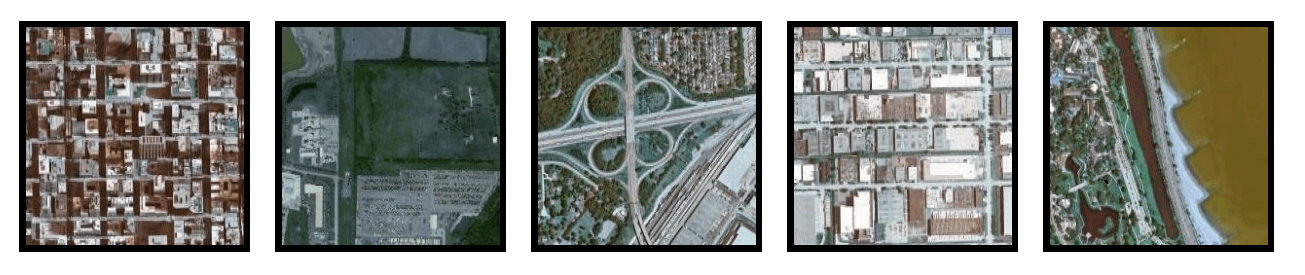
Figure 7: Image samples of cluster centers

Even though spatial information is not explicitly used as inputs, the clusters represent meaningful spatial patterns. As shown in Figure 8, the clusters have a geographical pattern that corresponds to the urban and suburban regions in Chicago. The clusters can be thought of as latent classes in traditional hybrid choice models. The latent space enables us to derive the five clusters because it is more general than the classical latent classes.

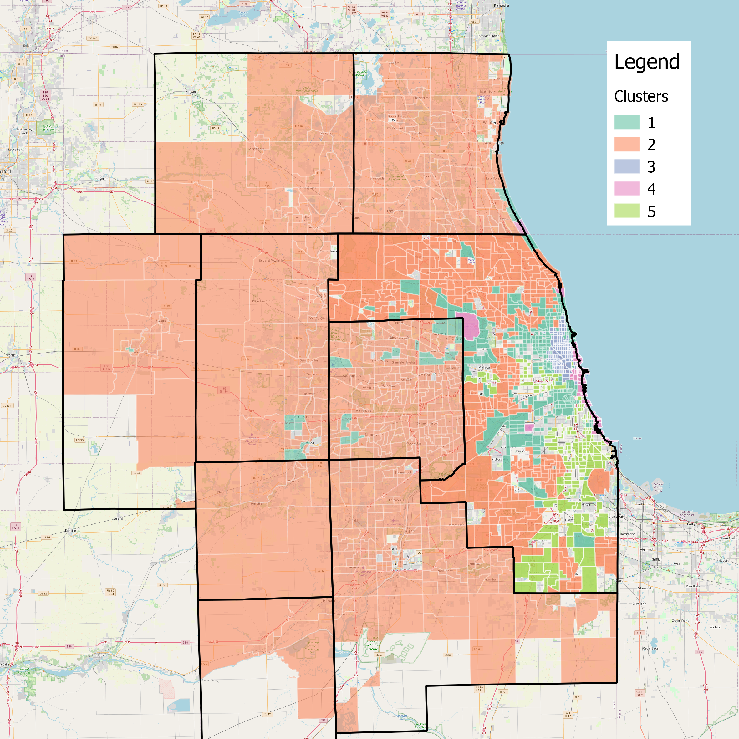
(a)

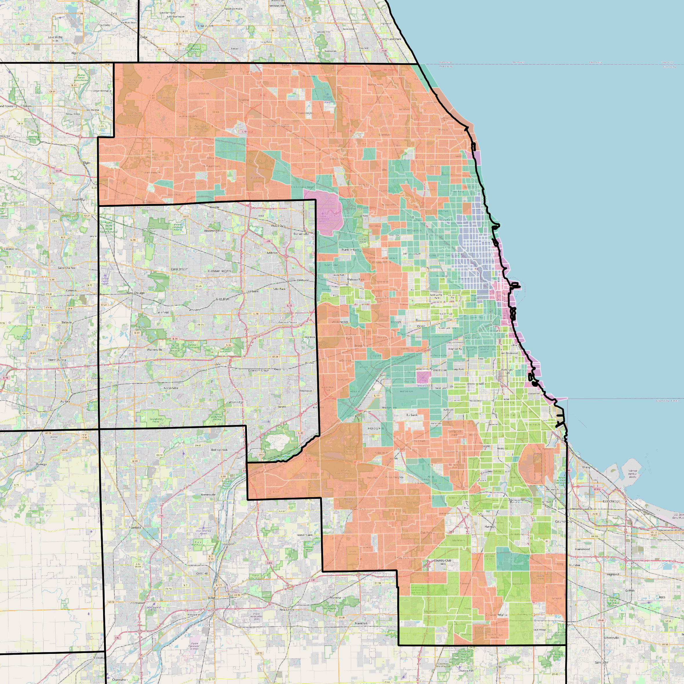
(b)

Figure 8: Spatial distribution of clusters

Besides discrete clusters, the latent space can represent continuous latent variables, approximating yet differing from the sociodemographic variables. Using t-distributed stochastic neighbor embedding (tSNE), the latent space is reduced to 2D for visualization, as shown in Figure 9. The latent space with labeled cluster centers is shown in Figure 9a, while the continuous sociodemographics in the latent space are plotted in Figure 9b-f. The sociodemographic transition patterns aligns with but also provide additional information to the discrete clusters. For example, the sociodemographics of the first cluster (downtown) are of high income, quite high population density, high percentage of adults and college graduates, and moderate to low travel time to work. The sociodemographics of the second cluster includes moderate income, low population density, moderate proportions of college graduates, and moderate travel time to work. These sociodemographic information in the latent space accurately reveal the social patterns in Chicago.

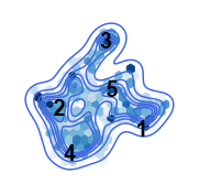
(a)

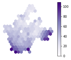
(b)

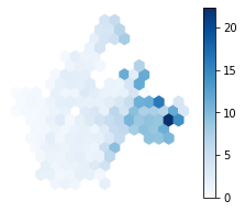
(c)

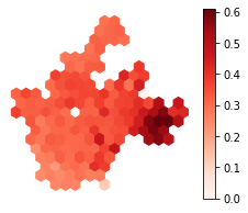
(d)

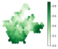
(e)

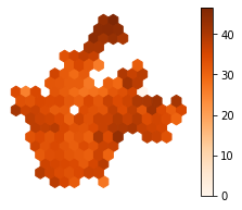
(f)

Figure 9: tSNE visualization of latent space

5.3 Economic interpretation of generated urban imagery

We demonstrate the economic interpretation by starting with existing satellite images from three census tracts (Figure 10), which represent diverse socioeconomic contexts in the South, North, and Central Chicago areas (Table 5). The first image is located in the south Chicago with a mixed urban texture and a major green area crossing the center. This area is associated with low income, low rates of college graduates and long commuting time. The other two images are located in the north suburban and the central Chicago areas. The north suburban region represents the high-income, low-density areas, while the central region is particularly dense and relatively wealthy. Regarding their urban texture, the northern image has a typical suburban pattern with curved roads and low-density buildings, while the central Chicago has the small-scale and grid-shaped building blocks. We denote the latent variables of the three census tracts in the south, north, and central Chicago as $z_{s}$, $z_{n}$, and $z_{c}$, and their corresponding images as $I_{s}$, $I_{n}$, and $I_{c}$.

Table 5: Sociodemographic characteristics of three census tracts

Census Tract	Pop Density (k-ppl/$km^{2}$)	% College Grad	Avg Time to Work (min)	Income (10k/capita)	Auto	PT	Active
South	2.5	10.7%	33.6	12.1	69.9%	15.4%	5.17%
North	1.0	78.2%	37.1	90.8	86.6%	5.1%	6.5%
Central	6.2	75.9%	28.0	70.8	12.0%	46.7%	38.4%

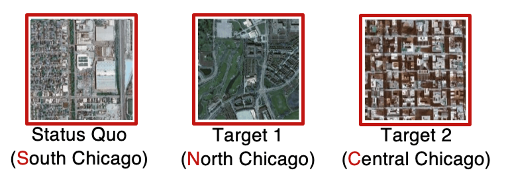
Figure 10: Satellite images of three census tracts

5.3.1 Economic interpretation with one-directional movement in the latent space

We first generate new urban images by using latent variable $\tilde{z}$ through the decoder $\tilde{I}=D_{\psi}({\tilde{z}})$ by interpolating between images from south Chicago $z_{s}$ and central Chicago $z_{c}$. Specifically, the latent variable $\tilde{z}$ can be created by adding a directional vector ${u}$ to the source latent variable ${z_{s}}$: $\tilde{z}=z_{s}+a_{1}u$, in which $a_{1}$ ranging from 0 to 1.6 in 0.2 increments, and $u$ being the difference between the target and source image $u=z_{c}-z_{s}$. As a result, regarding each $\tilde{z}$, a corresponding satellite image $\tilde{I}$ can be generated as shown in Figure 11. This linear formula $\tilde{z}=z_{s}+a_{1}u$ is quite flexible because it incorporates both image interpolation and extrapolation. Interpolation refers to the cases where $a_{1}<1$, while extrapolation refers to the cases where $a_{1}>1$. This linear formula also incorporates the two source images $z_{s}$ and $z_{c}$ as specific examples: when $a_{1}=0$, then ${\tilde{z}}={z_{s}}$, and when $a_{1}=1$, ${\tilde{z}}={z_{c}}$. In the two cases, the generated images are the same as $I_{s}$ and $I_{c}$.

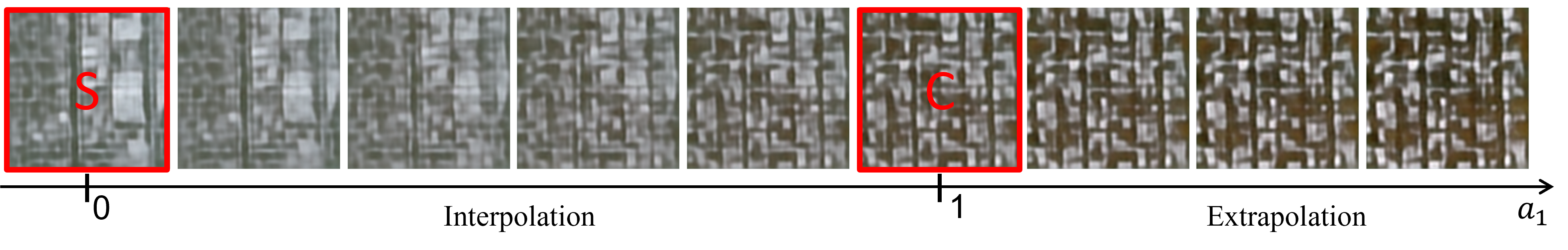
Figure 11: One-directional image generation

We also compute the economic information associated with the latent variable $\tilde{z}$, including travel behavior, utility values, and sociodemographic values by using $g(\tilde{z})$, $V_{nk}(\tilde{z})$, and $F_{\omega}(\tilde{z})$, all of which are learnt in the training of DHMs. Figure 12a-d demonstrate how market shares, social welfare, substitution patterns, and probability derivatives, and sociodemographics are associated with the latent variable $\tilde{z}$ by varying the scale factor $a_{1}$ from $0.0$ to $1.6$. We found that the economic information associated with the latent variables and the generated images appears reasonable. Specifically, the market shares, as computed by $e^{\beta_{k}^{\prime}\tilde{z}}/{\sum_{j}e^{\beta_{j}^{\prime}\tilde{z}}}$, demonstrate the decrease of auto mode when the latent variable moves from the central to the south Chicago. Social welfare, as computed by the logsum form $\frac{1}{\alpha_{n}}\log(\sum_{j}e^{\beta_{j}^{\prime}\tilde{z}})$, indicates that the minimum logsum is achieved when the utilities of all modes are roughly equivalent. The directional probability derivative $\nabla_{u}P_{nk}$, as visualized in Figure 12d, demonstrates that the choice probability derivatives are marginally decreasing when one product starts to dominate the market. While we could provide much finer economic interpretation through our approach, it is critical to note the main innovation: through the latent variable $\tilde{z}$, we can attach the generated satellite images $\tilde{I}$ (Figure 11) to the corresponding economic information (Figure 12), thus rendering satellite images at least partially interpretable in an economic manner.

With the same reasoning, each generated image is associated with predicted sociodemographics via $F_{\omega}({\tilde{z}})$. Figure 12e demonstrates how the predicted sociodemographics vary with the latent variable $\tilde{z}$ and correspondingly the generated urban image $\tilde{I}$. Comparing the predicted sociodemographic values with the observed ones in Table 5, the majority of these values are similar. When $a_{1}$ increases, there is a increasing number of young adults (25-34yrs), white people, college graduates, and income, while the travel time to work decreases. Since $\tilde{z}$ is uniquely associated with the generated satellite image $\tilde{I}$, the predicted values in Figure 12e could be used to characterize the sociodemographic features of the urban environment as shown by the generated satellite images in Figure 11.

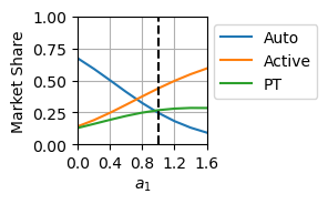
(a)

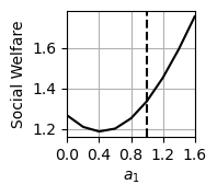
(b)

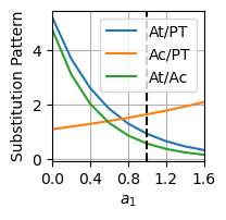
(c)

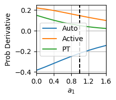
(d)

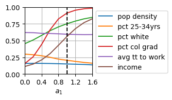
(e)

Figure 12: Economic information of images generated along one direction (S to C: $\tilde{z}=z_{s}+a_{1}(z_{c}-z_{s})$)

5.3.2 Economic interpretation with two-directional movement in the latent space

We generate new satellite images with $\tilde{I}=D_{\psi}({\tilde{z}})$ by extending the one-directional to a two-directional analysis using ${\tilde{z}}=a_{1}{u_{1}}+a_{2}{u_{2}}=a_{1}({z_{c}-z_{s}})+a_{2}({z_{n}-z_{s}})$. In this formula, two directions are defined by $z_{c}-z_{s}$ and $z_{n}-z_{s}$, representing the movement from the south Chicago to north and central Chicago in the latent space. Figure 13 visualizes a 9 $\times$ 9 matrix of the interpolated and extrapolated images using the three existing urban images from Figure 10. The image matrix has in total 81 images, among which only three images (S, N, and C) exist in reality while the other 78 images are generated. The 78 generated urban images are not only visually recognizable but also present semantically meaningful urban planning features. For example, moving from the south to north Chicago, the major north-south green belt is gradually replaced by the curved suburban roads and low-density buildings. Moving from the south to central Chicago, the grid structure and dense buildings gradually dominate. In the extrapolated images, the characteristics of the target images (north and center Chicago) are amplified: on the vertical axis, the green color gets deepened, and on the horizontal axis, the buildings are densified. This approach of image generation along two directions is generally applicable, as shown by another example in Appendix IV.

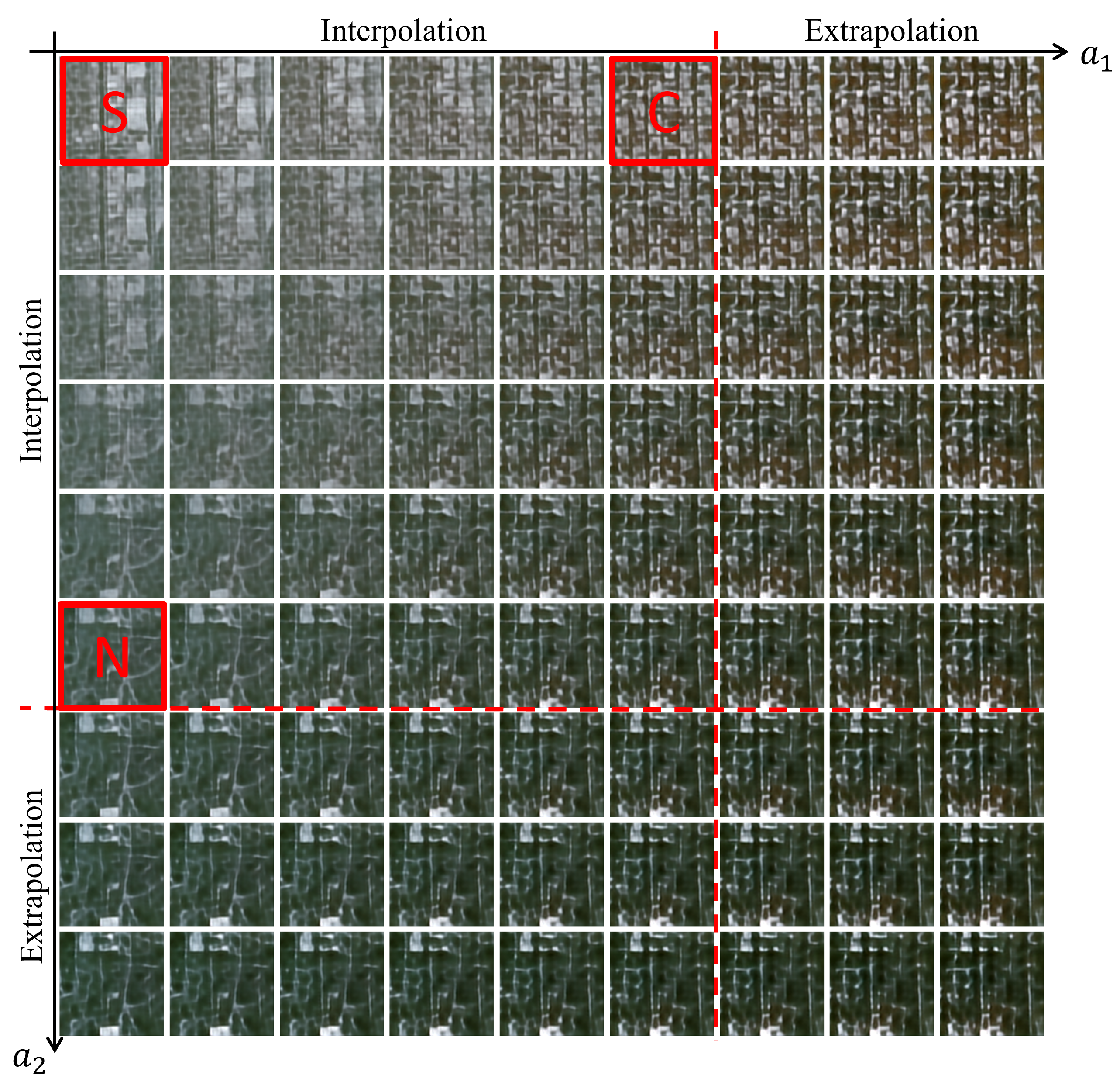
Figure 13: Two-directional image generation

Each generated satellite image $\tilde{I}=D_{\psi}({\tilde{z}})$ in Figure 13 can be interpreted in an economic manner by using the latent variable $\tilde{z}$ and the trained functions $g(\tilde{z})$, $V_{nk}(\tilde{z})$, and $F_{\omega}(z)$. Figure 14 visualizes social welfare and market shares for each satellite image in the image matrix (Figure 13), with the same 9 $\times$ 9 size. In other words, each satellite image on row $i$ and column $j$ in Figure 13 is corresponding to the market share and social welfare values in the pixel on row $i$ and column $j$ in Figure 14. While one-directional plot provides insights into a nonlinear relationship between latent space and socioeconomic outputs (Figure 12), the matrix plots provide a holistic view for the two-directional interactions (Figure 14). For example, it does not affect public transit usage by moving from south to north Chicago , whereas it does so by moving from south to central Chicago in the latent space. Although it is possible to compute a full set of economic parameters for latent variable $\tilde{z}$ and the corresponded image $\tilde{I}$, we only demonstrate the feasibility of our approach by visualizing market shares and social welfare. It is more important to recognize the power of the DHMs through the one-directional and two-directional examples: with the latent variable $\tilde{z}$ centered in DHMs, we could regenerate new satellite image $\tilde{I}$, and associate with it the economic meanings by using $g(\tilde{z})$, $V_{nk}(\tilde{z})$, and $F_{\omega}(\tilde{z})$ functions.

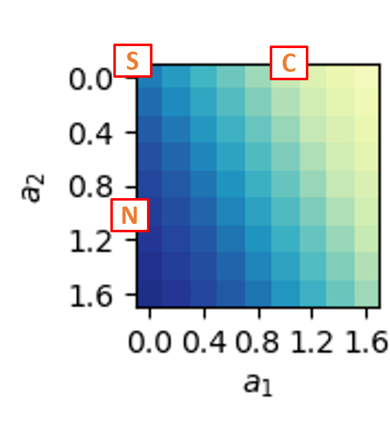
(a)

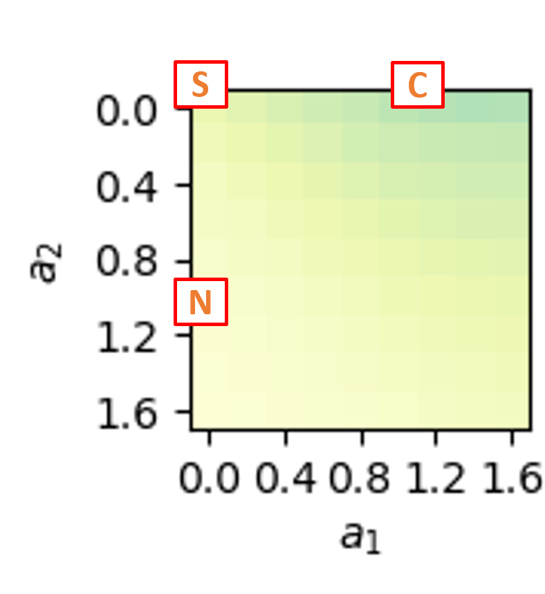
(b)

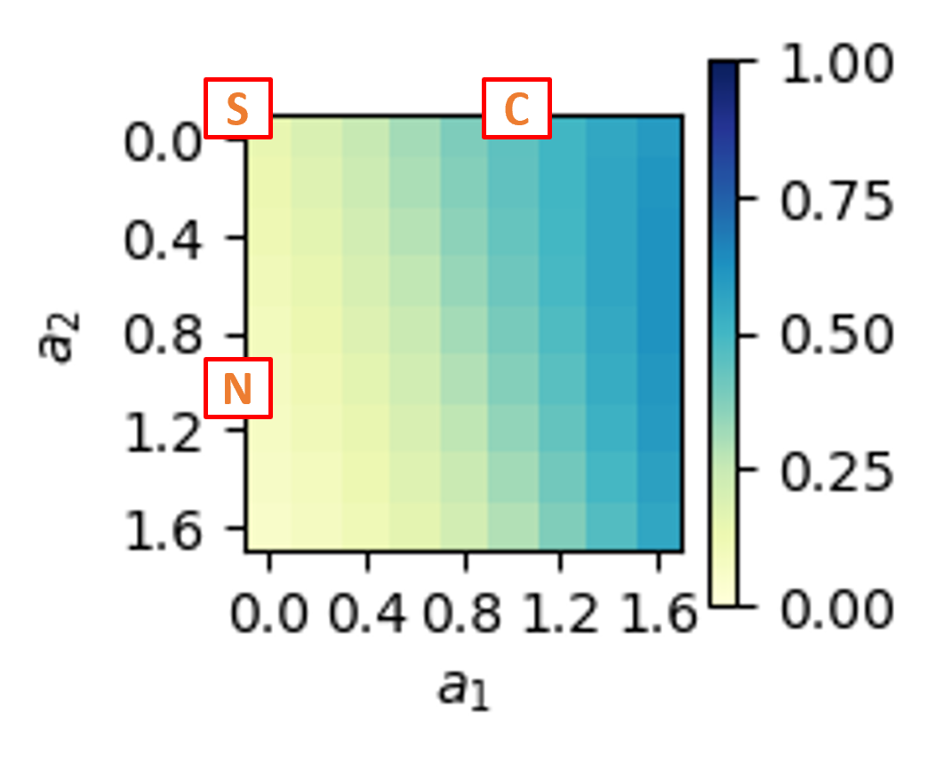
(c)

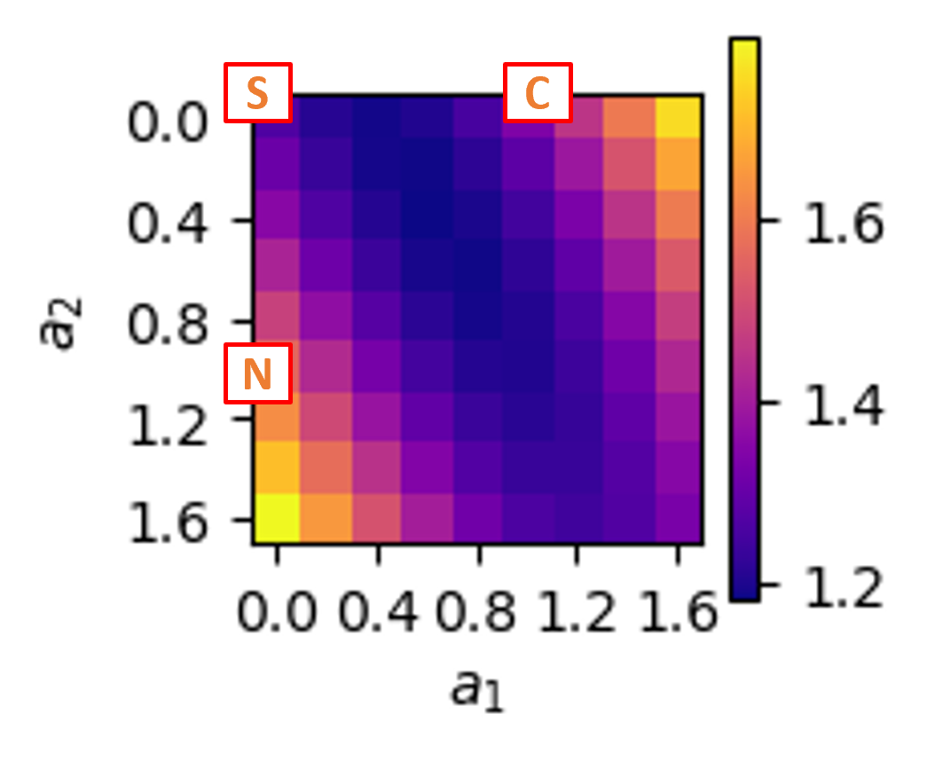
(d)

Figure 14: Economic information of images generated along two directions

6 Conclusion

Travel decisions can be influenced by the factors represented by either numeric data or urban imagery. Although classical demand modeling is incapable of processing urban imagery, it becomes an imperative to expand on this capacity given the explosion of unstructured data and the power of deep learning. This study proposes the DHM framework to integrate numeric and urban imagery by combining the analytical capacity of the classical demand modeling and the computational capacity of the DNNs. After empirically examining its performance, we demonstrate three major findings of DHMs, which are corresponding to three contributions of this research.

The first contribution is demonstrating the complementarity in data and model. The data complementarity is demonstrated through the higher performance of the DHMs combining numeric and imagery data over the benchmark models using only sociodemographics or only urban imagery. The model complementarity is demonstrated by the successful integration of the classical demand modeling and deep learning through the latent space in the DHMs. Technically, the complementarity is achieved by the supervision-as-mixing design in the mixing operator. In contrast to the simple concatenation, supervision-as-mixing combines the imagery and sociodemographics in the latent neurons, which are found to be more generalizable than the neurons in the baseline autoencoder. The second contribution is creating a latent space that generalizes the concept of latent variables and classes in the classical hybrid demand models [4]. This urban imagery latent space is interpretable, because it contains meaningful social and spatial characteristics. It is more general than the latent variables and classes because it can encode diverse and rich information from unstructured data. The third contribution is generating urban imagery with economic interpretation. The DHMs can generate new urban imagery through the linear transformation in the latent space. The economic parameters of the generated urban images (e.g. mode shares and social welfare) can be computed because the latent space successfully associates sociodemographics, trip attributes, and behavioral outputs with urban imagery. This economic interpretation of images is possible only because both the analytical capacity of demand modeling and the computational capacity of deep learning coexist in the DHMs. The economic interpretation also transcends a simple image generation because it allows us to examine the social consequences of the newly generated urban landscape.

Our framework can be understood as hybrid in five different perspectives. Three perspectives are already fully elaborated above: it is hybrid because it integrates numeric and imagery data, it combines classical demand modeling and deep learning, and it resembles the classical hybrid model in its crossing structure with the measurement and the structure model. Two other perspectives, relatively less elaborated in the discussions above, are on the machine learning side. The DHMs are hybrid because it mixes the supervised and unsupervised learning: the vertical axis of DHMs in Figure 1 represents supervised learning, while the horizontal autoencoder represents the unsupervised learning. It also mixes the discriminative and generative methods: the decoder generates new urban imagery while the behavioral prediction is discriminative. The two perspectives are explained in detail in many machine learning studies that adopted the hybrid generative-discriminative or supervised-unsupervised methods [71, 72, 73, 74]. Readers could refer to these studies to improve the DHMs from the machine learning perspectives.

Although the DHM framework is presented mainly as an innovation in modeling, it also provides a prototype for automating urban planning in practice. One hallmark of urban planning is the generation of new urban plans, which are often represented by urban imagery, with detailed elaboration on the social, behavioral, and economic consequences. This DHM framework already achieves this basic goal because it can generate new urban images and simultaneously associate them with social, behavioral, and economic implications. Although our work is still far away from achieving the full automation of urban planning, we believe it is an important first step for the future AI-based planning practice.

The DHM framework is not devoid of limitations. Because of the central role of the mixing operator and the latent space in DHMs, we encourage researchers to explore new approaches to design the mixing operator to effectively integrate multiple data structures to further improve the predictive performance. Currently, the deep learning components in DHMs rely on autoencoder, which tends to generate blurry images that may not be satisfactory for practical use. This weakness could be mitigated by further enhancing the autoencoder (e.g. variational autoencoder) or adopting another framework (e.g. generative adversarial model). Besides the mixing operator, the DHMs use simple linear transformations for multiple purposes, including aggregating information for a census tract and exploring the latent space for image generation. The simple linear transformation might not be the optimum approach to achieve these goals. Researchers could also explore the usefulness of satellite imagery in different contexts. For example, sociodemographics are often considered the exogenous variables for energy consumption, health, and air pollution, so future research could combine satellite imagery with sociodemographics to analyze these factors through the DHM framework. However, satellite imagery, regardless of its spatial resolution, inherently represents aggregate information, which might provide less valuable information than the street view images. Since our work has laid out a base structure to combine sociodemographics and imagery, it is feasible to adopt the DHMs to combine drivers’ attributes and street view imagery to predict individualized driving behavior.

CRediT authorship contribution statement

Qingyi Wang: Conceptualization, Methodology, Software, Data Curation, Writing - Original Draft, Writing - Review & Editing, Visualization; Shenhao Wang: Conceptualization, Methodology, Writing - Original Draft, Writing - Review & Editing, Supervision, Project administration, Funding acquisition; Yunhan Zheng: Writing - Review & Editing; Hongzhou Lin: Conceptualization; Xiaohu Zhang: Data Curation; Jinhua Zhao: Supervision, Funding acquisition; Joan Walker: Supervision. The authors declare no conflict of interest.

Appendix I. Specific model design in disaggregate analysis

To simplify the notation used in the manuscript, we only distinguish between imagery latent variables and numeric vairables in our discussion. In fact, there are three types of inputs to the behavioral predictors: imagery latent variables, sociodemographics, and alternative-specific variables. Both sociodemographics and alternative-specfic variables are numeric but they enter the utility function slightly differently. In this paper, we used $z_{n}$ to represent the imagery latent space, $x^{sd}$ and $x^{alt}$ represent the sociodemographic and alternative-specific attributes, respectively. Combining all three types of attributes, we formulate the utility function as follows:

$$V_{nk}=\beta^{im^{\prime}}_{k}z_{n}+\beta^{sd^{\prime}}_{k}x^{sd}_{n}+\beta^{alt^{\prime}}x^{alt}_{nk}$$ (14)

where $\beta^{im^{\prime}}_{k}$, $\beta^{sd^{\prime}}_{k}$, and $\beta^{alt^{\prime}}$ are vector coefficients of urban imagery latent space, sociodemographics, and alternative-specific attributes, respectively. We assume that the alternative-specific variables share the same coefficients in the utility of all alternatives. Both imagery and sociodemographics are not alternative-specific, therefore the coefficients $\beta^{im^{\prime}}_{k}$, $\beta^{sd^{\prime}}_{k}$ are alternative-specific to distinguish the effect these variables have on different alternatives.

Depending on the dataset and task, different types of variables exist. In this paper, in the aggregate models, the types of inputs available to Model 1-6 are, $x^{sd}$, $z$, $x^{sd}$, $z$, [$x^{sd},z$], and [$x^{sd},z$] respectively. In the disaggregate models, we append $x^{alt}$, which is the trip-level alternative-specific attributes to every model.

In Section 3.5, we also discussed the directional probability derivatives for the imagery latent variable $z_{n}$. We could also calculate probability derivatives for the other two types of variables. Both sociodemographic and alternative-specific variables are standard numeric variables and many references exist on the how to get the probability derivatives. We only summarize the results below.

For alternative-specific attributes, the probability derivative, which is the change in probability that a trip $n$ uses alternative $k$ with respect to changes in variable $i$ is simply

$$\frac{\partial P_{nk}}{\partial x^{alt}_{nki}}=\frac{\partial V_{nk}}{\partial x^{alt}_{nki}}P_{nk}(1-P_{nk})=\beta^{alt}_{i}P_{nk}(1-P_{nk})$$ (15)

Sociodemographics variables enter the utility of all alternatives with different $\beta$ parameters. Therefore the change in probability that a trip $n$ uses alternative $k$ with respect to changes in variable $i$ is

$$\frac{\partial P_{nk}}{\partial x^{sd}_{ni}}=\sum_{k^{\prime}}\frac{\partial P_{nk}}{\partial V_{nk^{\prime}}}\frac{\partial V_{nk^{\prime}}}{\partial x^{sd}_{ni}}=\beta^{sd}_{ki}P_{nk}(1-P_{nk})-\sum_{k^{\prime}}{\beta^{sd}_{k^{\prime}i}P_{nk}P_{nk^{\prime}}}$$ (16)

We can compute a directional gradient of choice probabilities regarding the imagery latent space, which resembles but also differs from the marginal effects $\beta$ in the classical demand modeling. The formula of the directional gradient is

$$\nabla_{u}P_{nk}({z})={u}\cdot\nabla P_{nk}({z})=\sum_{k^{\prime}}\frac{\partial P_{nk}}{\partial V_{nk^{\prime}}}\nabla_{u}V_{nk^{\prime}}({z_{n}})={u}\cdot({\beta^{im}_{k}}P_{nk}(1-P_{nk})-\sum_{k^{\prime}}{{\beta^{im}_{k^{\prime}}}P_{nk}P_{nk^{\prime}}})$$ (17)

Appendix II. Predictive performance with cross validation

Table A1: Cross-validated predictive performance of aggregate travel behavior predictors

	1	2	3	4	5	6
	SD	IM	SSD	SIM	C[SD-IM]	C[SD-IM-SSD-SIM]
Panel 1: Aggregate Mode Choice as Separate Outputs - Linear Regression
Input Dim	10	18432	10	18432	10+18432	10*2+18432*2
Auto ($R^{2}$)	0.55/0.54	0.63/0.53	0.59/0.59	0.70/0.62	0.66/0.59	0.71/0.62
Active ($R^{2}$)	0.46/0.45	0.55/0.74	0.48/0.47	0.59/0.49	0.56/0.47	0.59/0.48
PT ($R^{2}$)	0.43/0.42	0.50/0.39	0.47/0.46	0.57/0.48	0.54/0.46	0.56/0.49
Panel 2: Aggregate Mode Choice as a Joint Output - Multinomial Regression
Input Dim	10	18432	10	18432	10+18432	10*2+18432*2
KL Loss	0.153/0.155	0.148/0.158	0.145/0.146	0.105/0.135	0.135/0.146	0.103/0.134
Auto ($R^{2}$)	0.51/0.55	0.51/0.48	0.54/0.54	0.73/0.62	0.60/0.56	0.74/0.62
Active ($R^{2}$)	0.42/0.41	0.43/0.40	0.43/0.42	0.65/0.49	0.50/0.45	0.66/0.49
PT ($R^{2}$)	0.39/0.37	0.40/0.36	0.44/0.44	0.68/0.47	0.48/0.43	0.66/0.49
Note: each entry is represented as training/testing performance.

This table adopts a format similar to Table 2, but skips Panel 3 that requires high computational costs at the individual level. With cross validation, we observe a slight drop in predictive performance of the DHMs; however, the DHMs still achieve the highest predictive performance, which aligns with the main findings in Table 2. It validates our main hypothesis that a hybrid approach can outperform the models using only socio-demographics and only urban imagery.

Appendix III. Controlling the quality of image reconstruction

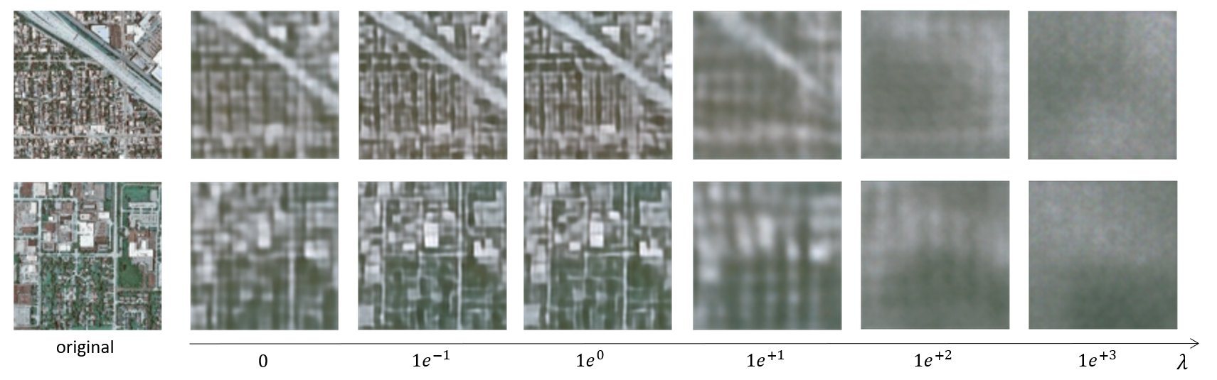
Figure A1: Quality of image reconstruction with varying $\lambda$ values

This figure visualizes the quality of original urban images, reconstructured images with the baseline autoencoder, and the reconstructured images with varying $\lambda$ values using two example satellite images. Overall, with a higher $\lambda$ value, it is more likely to observe a blurry reconstructed urban imagery. This result is consistent with the design of the model, since higher $\lambda$ values shift the training focuses on the prediction of socio-demographics rather than reconstruction of urban images. Meanwhile, baseline autoencoders are more likely to generate blurry images comparing to other alternatives (e.g., GAN), as demonstrated in Figure A1.

Appendix IV. two-directional imagery regeneration

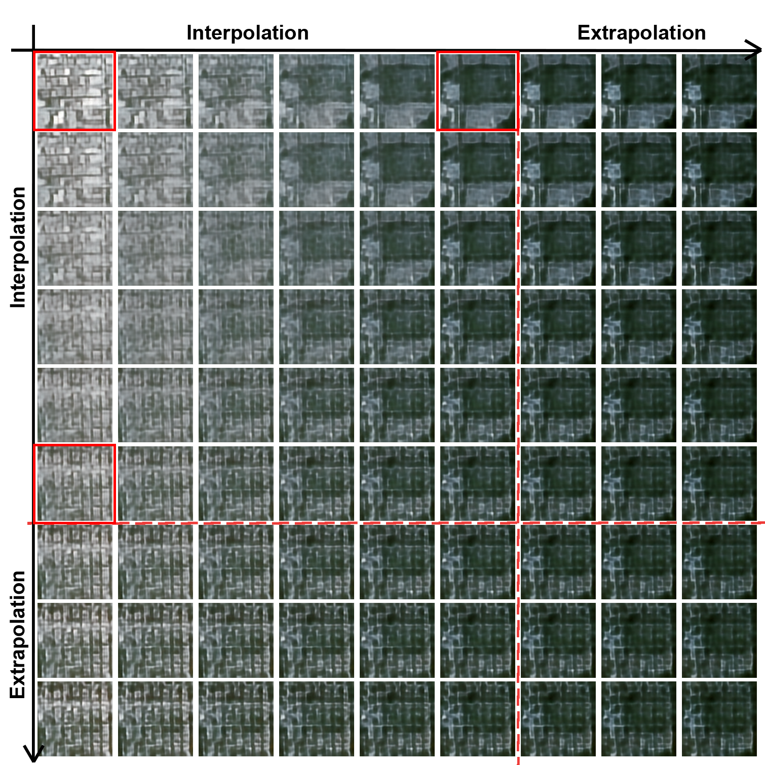
Figure A2: Another example of 2D directional image regeneration with economic interpretation

This figure demonstrates another example of reconstructing satellite images with the 2D directional movements in the latent space. Similar to Figure 13, we choose three targeting images, as highlighted by the red squares, to generate new urban images by liner interpolation and extrapolation in the latent space. The images appear realistic, and through our framework, they are also associated with socioeconomic and behavioral information.

References

- [1] Daniel McFadden “Conditional logit analysis of qualitative choice behavior”, 1974
- [2] Daniel McFadden “Modeling the choice of residential location” In Transportation Research Record, 1978
- [3] Daniel McFadden and Kenneth Train “Mixed MNL models for discrete response” In Journal of applied Econometrics 15.5, 2000, pp. 447–470
- [4] Joan Walker and Moshe Ben-Akiva “Generalized random utility model” In Mathematical social sciences 43, 2002, pp. 303–343 DOI: 10.1016/S0165-4896(02)00023-9
- [5] Moshe Ben-Akiva et al. “Hybrid Choice Models: Progress and Challenges” In Marketing Letters 13, 2002, pp. 163–175
- [6] Akshay Vij and Joan L. Walker “How, when and why integrated choice and latent variable models are latently useful” In Transportation Research Part B: Methodological 90 Pergamon, 2016, pp. 192–217 DOI: 10.1016/J.TRB.2016.04.021
- [7] Kenneth Train “A structured logit model of auto ownership and mode choice” In The Review of Economic Studies 47.2, 1980, pp. 357–370
- [8] John Paul Helveston et al. “Will subsidies drive electric vehicle adoption? Measuring consumer preferences in the US and China” In Transportation Research Part A: Policy and Practice 73, 2015, pp. 96–112
- [9] Angela Stefania Bergantino, Mauro Capurso and Stephane Hess “Modelling regional accessibility to airports using discrete choice models: An application to a system of regional airports” In Transportation Research Part A: Policy and Practice 132, 2020, pp. 855–871
- [10] Neal Jean et al. “Combining satellite imagery and machine learning to predict poverty” In Science 353.6301, 2016, pp. 790–794 DOI: 10.1126/science.aaf7894
- [11] Kumar Ayush et al. “Generating interpretable poverty maps using object detection in satellite images” In IJCAI International Joint Conference on Artificial Intelligence 2021-Janua, 2020, pp. 4410–4416 DOI: 10.24963/ijcai.2020/608
- [12] Christopher Yeh et al. “Using publicly available satellite imagery and deep learning to understand economic well-being in Africa” In Nature Communications 11.1 Springer US, 2020, pp. 1–11 DOI: 10.1038/s41467-020-16185-w
- [13] Kenneth A Small and Harvey S Rosen “Applied welfare economics with discrete choice models” In Econometrica: Journal of the Econometric Society, 1981, pp. 105–130
- [14] Luca Zamparini and Aura Reggiani “The value of travel time in passenger and freight transport: an overview” In Policy analysis of transport networks Routledge, 2016, pp. 161–178
- [15] Poopak Azad, Nima Jafari Navimipour, Amir Masoud Rahmani and Arash Sharifi “The role of structured and unstructured data managing mechanisms in the Internet of things” In Cluster Computing 23.2, 2020, pp. 1185–1198
- [16] Timnit Gebru et al. “Using deep learning and google street view to estimate the demographic makeup of neighborhoods across the United States” In Proceedings of the National Academy of Sciences of the United States of America 114.50, 2017, pp. 13108–13113 DOI: 10.1073/pnas.1700035114
- [17] Shenhao Wang, Baichuan Mo and Jinhua Zhao “Deep neural networks for choice analysis: Architecture design with alternative-specific utility functions” In Transportation Research Part C: Emerging Technologies 112 Pergamon, 2020, pp. 234–251 DOI: 10.1016/J.TRC.2020.01.012
- [18] Shenhao Wang, Qingyi Wang and Jinhua Zhao “Deep neural networks for choice analysis: Extracting complete economic information for interpretation” In Transportation Research Part C: Emerging Technologies 118 Elsevier, 2020, pp. 102701
- [19] Shenhao Wang, Qingyi Wang, Nate Bailey and Jinhua Zhao “Deep neural networks for choice analysis: A statistical learning theory perspective” In Transportation Research Part B: Methodological 148, 2021, pp. 60–81 DOI: 10.1016/j.trb.2021.03.011
- [20] Ning Huan, Stephane Hess and Enjian Yao “Understanding the effects of travel demand management on metro commuters’ behavioural loyalty: a hybrid choice modelling approach” In Transportation Springer, 2021, pp. 1–30 DOI: 10.1007/S11116-021-10179-3/FIGURES/7
- [21] Yunhan Zheng, Shenhao Wang and Jinhua Zhao “Equality of opportunity in travel behavior prediction with deep neural networks and discrete choice models” In Transportation Research Part C: Emerging Technologies 132 Elsevier, 2021, pp. 103410
- [22] Aurélie Glerum, Lidija Stankovikj, Michaël Thémans and Michel Bierlaire “Forecasting the Demand for Electric Vehicles: Accounting for Attitudes and Perceptions” HCM application In https://doi.org/10.1287/trsc.2013.0487 48 INFORMS, 2013, pp. 483–499 DOI: 10.1287/TRSC.2013.0487
- [23] Shenhao Wang and Jinhua Zhao “Risk preference and adoption of autonomous vehicles” In Transportation research part A: policy and practice 126 Elsevier, 2019, pp. 215–229
- [24] Prateek Bansal, Kara M Kockelman and Amit Singh “Assessing public opinions of and interest in new vehicle technologies: An Austin perspective” In Transportation Research Part C: Emerging Technologies 67 Elsevier, 2016, pp. 1–14
- [25] Basil Schmid and Kay W. Axhausen “In-store or online shopping of search and experience goods: A hybrid choice approach” In Journal of Choice Modelling 31 Elsevier, 2019, pp. 156–180 DOI: 10.1016/J.JOCM.2018.03.001
- [26] Muhammad Zudhy Irawan, Prawira Fajarindra Belgiawan, Tri Basuki Joewono and Nurvita I.M. Simanjuntak “Do motorcycle-based ride-hailing apps threaten bus ridership? A hybrid choice modeling approach with latent variables” In Public Transport 12 Springer, 2020, pp. 207–231 DOI: 10.1007/S12469-019-00217-W/TABLES/8
- [27] Giulio Erberto Cantarella and Stefano de Luca “Multilayer feedforward networks for transportation mode choice analysis: An analysis and a comparison with random utility models” Handling Uncertainty in the Analysis of Traffic and Transportation Systems (Bari, Italy, June 10–13 2002) In Transportation Research Part C: Emerging Technologies 13.2, 2005, pp. 121–155 DOI: https://doi.org/10.1016/j.trc.2005.04.002
- [28] Dongwoo Lee, Sybil Derrible and Francisco Camara Pereira “Comparison of four types of artificial neural network and a multinomial logit model for travel mode choice modeling” In Transportation Research Record 2672.49 SAGE Publications Sage CA: Los Angeles, CA, 2018, pp. 101–112
- [29] Tim Hillel, Michel Bierlaire, Mohammed Z.E.B. Elshafie and Ying Jin “A systematic review of machine learning classification methodologies for modelling passenger mode choice” In Journal of Choice Modelling 38 Elsevier, 2021, pp. 100221 DOI: 10.1016/J.JOCM.2020.100221
- [30] Sander Cranenburgh et al. “Choice modelling in the age of machine learning - Discussion paper” In Journal of Choice Modelling 42 Elsevier, 2022, pp. 100340 DOI: 10.1016/J.JOCM.2021.100340
- [31] Yuankai Wu, Dingyi Zhuang, Aurelie Labbe and Lijun Sun “Inductive Graph Neural Networks for Spatiotemporal Kriging” In Proceedings of the AAAI Conference on Artificial Intelligence 35.5, 2021, pp. 4478–4485 URL: https://ojs.aaai.org/index.php/AAAI/article/view/16575
- [32] Yuankai Wu et al. “Spatial Aggregation and Temporal Convolution Networks for Real-time Kriging” In arXiv preprint arXiv:2109.12144, 2021
- [33] Dingyi Zhuang, Siyu Hao, Der-Horng Lee and Jian Gang Jin “From compound word to metropolitan station: Semantic similarity analysis using smart card data” In Transportation Research Part C: Emerging Technologies 114 Elsevier, 2020, pp. 322–337
- [34] Dingyi Zhuang, Shenhao Wang, Haris Koutsopoulos and Jinhua Zhao “Uncertainty Quantification of Sparse Travel Demand Prediction with Spatial-Temporal Graph Neural Networks” In Proceedings of the 28th ACM SIGKDD Conference on Knowledge Discovery and Data Mining, 2022, pp. 4639–4647
- [35] Fuqiang Liu et al. “A Universal Framework of Spatiotemporal Bias Block for Long-Term Traffic Forecasting” In IEEE Transactions on Intelligent Transportation Systems IEEE, 2022
- [36] M.. Karlaftis and E.. Vlahogianni “Statistical methods versus neural networks in transportation research: Differences, similarities and some insights” comprehensive comparison of NN and statistical methods both in terms of philosophy and transportation applications. In Transportation Research Part C: Emerging Technologies 19 Elsevier Ltd, 2011, pp. 387–399 DOI: 10.1016/J.TRC.2010.10.004
- [37] Miguel Paredes, Erik Hemberg, Una-May O’Reilly and Chris Zegras “Machine learning or discrete choice models for car ownership demand estimation and prediction?” In 2017 5th IEEE International Conference on Models and Technologies for Intelligent Transportation Systems (MT-ITS), 2017, pp. 780–785 IEEE
- [38] Tim Hillel “New perspectives on the performance of machine learning classifiers for mode choice prediction”, 2020
- [39] Sander Cranenburgh and Marco Kouwenhoven “An artificial neural network based method to uncover the value-of-travel-time distribution” In Transportation 48.5 Springer, 2021, pp. 2545–2583
- [40] Ahmad Alwosheel, Sander Cranenburgh and Caspar G Chorus “Why did you predict that? Towards explainable artificial neural networks for travel demand analysis” In Transportation Research Part C: Emerging Technologies 128 Elsevier, 2021, pp. 103143
- [41] Melvin Wong and Bilal Farooq “ResLogit: A residual neural network logit model for data-driven choice modelling” In Transportation Research Part C: Emerging Technologies 126 Elsevier, 2021, pp. 103050
- [42] Shenhao Wang, Baichuan Mo and Jinhua Zhao “Theory-based residual neural networks: A synergy of discrete choice models and deep neural networks” In Transportation Research Part B: Methodological 146 Pergamon, 2021, pp. 333–358 DOI: 10.1016/J.TRB.2021.03.002
- [43] Brian Sifringer, Virginie Lurkin and Alexandre Alahi “Enhancing discrete choice models with representation learning” In Transportation Research Part B: Methodological 140 Elsevier Ltd, 2020, pp. 236–261 DOI: 10.1016/j.trb.2020.08.006
- [44] Sander Cranenburgh and Ahmad Alwosheel “An artificial neural network based approach to investigate travellers’ decision rules” In Transportation Research Part C: Emerging Technologies 98 Elsevier, 2019, pp. 152–166
- [45] Rui Yao and Shlomo Bekhor “A variational autoencoder approach for choice set generation and implicit perception of alternatives in choice modeling” In Transportation Research Part B: Methodological 158 Elsevier, 2022, pp. 273–294
- [46] Melvin Wong and Bilal Farooq “Modelling latent travel behaviour characteristics with generative machine learning” In 2018 21st International Conference on Intelligent Transportation Systems (ITSC), 2018, pp. 749–754 IEEE
- [47] Yafei Han, Christopher Zegras, Francisco Camara Pereira and Moshe Ben-Akiva “A neural-embedded choice model: Tastenet-mnl modeling taste heterogeneity with flexibility and interpretability” In arXiv preprint arXiv:2002.00922, 2020
- [48] Ioanna Arkoudi, Carlos Lima Azevedo and Francisco C. Pereira “Combining Discrete Choice Models and Neural Networks through Embeddings: Formulation, Interpretability and Performance”, 2021 DOI: 10.48550/arxiv.2109.12042
- [49] Adrian Albert, Jasleen Kaur and Marta C González “Using Convolutional Networks and Satellite Imagery to Identify Patterns in Urban Environments at a Large Scale”, 2017 DOI: 10.1145/3097983.3098070
- [50] Ian Seiferling, Nikhil Naik, Carlo Ratti and Raphäel Proulx “Green streets - Quantifying and mapping urban trees with street-level imagery and computer vision” In Landscape and Urban Planning 165.July 2016, 2017, pp. 93–101 DOI: 10.1016/j.landurbplan.2017.05.010
- [51] Nikhil Naik et al. “Computer vision uncovers predictors of physical urban change” In Proceedings of the National Academy of Sciences of the United States of America 114.29, 2017, pp. 7571–7576 DOI: 10.1073/pnas.1619003114
- [52] Sean M. Arietta et al. “City Forensics: Using Visual Elements to Predict Non-Visual City Attributes” In IEEE Transactions on Visualization and Computer Graphics, 2014 DOI: 10.1109/tvcg.2014.2346446
- [53] Yulu Chen, Rongjun Qin, Guixiang Zhang and Hessah Albanwan “Spatial temporal analysis of traffic patterns during the covid-19 epidemic by vehicle detection using planet remote-sensing satellite images” In Remote Sensing 13.2 MDPI AG, 2021, pp. 1–18 DOI: 10.3390/rs13020208
- [54] Steve Hankey et al. “Predicting bicycling and walking traffic using street view imagery and destination data” In Transportation research part D: transport and environment 90 Elsevier, 2021, pp. 102651
- [55] Mohamed R. Ibrahim, James Haworth and Tao Cheng “Understanding cities with machine eyes: A review of deep computer vision in urban analytics” In Cities 96 Pergamon, 2020, pp. 102481 DOI: 10.1016/J.CITIES.2019.102481
- [56] Filip Biljecki and Koichi Ito “Street view imagery in urban analytics and GIS: A review” In Landscape and Urban Planning 215 Elsevier B.V., 2021, pp. 104217 DOI: 10.1016/J.LANDURBPLAN.2021.104217
- [57] Nikhil Naik, Jade Philipoom, Ramesh Raskar and César Hidalgo “Streetscore-predicting the perceived safety of one million streetscapes” In Proceedings of the IEEE conference on computer vision and pattern recognition workshops, 2014, pp. 779–785
- [58] Abhimanyu Dubey et al. “Deep learning the city: Quantifying urban perception at a global scale” In European conference on computer vision, 2016, pp. 196–212 Springer
- [59] Fan Zhang et al. “Measuring human perceptions of a large-scale urban region using machine learning” In Landscape and Urban Planning 180 Elsevier, 2018, pp. 148–160
- [60] Dumitru Erhan, Yoshua Bengio, Aaron Courville and Pascal Vincent “Visualizing higher-layer features of a deep network” In Technical Report, 2009, pp. 1–13 URL: http://igva2012.wikispaces.asu.edu/file/view/Erhan+2009+Visualizing+higher+layer+features+of+a+deep+network.pdf
- [61] Jost Tobias Springenberg, Alexey Dosovitskiy, Thomas Brox and Martin Riedmiller “Striving for simplicity: The all convolutional net” In 3rd International Conference on Learning Representations, ICLR 2015 - Workshop Track Proceedings, 2015
- [62] Ramprasaath R Selvaraju et al. “Grad-CAM: Visual Explanations from Deep Networks via Gradient-based Localization” URL: https://github.com/
- [63] Saining Xie et al. “Aggregated residual transformations for deep neural networks” In Proceedings - 30th IEEE Conference on Computer Vision and Pattern Recognition, CVPR 2017 2017-Janua, 2017, pp. 5987–5995 DOI: 10.1109/CVPR.2017.634
- [64] Kaiming He, Xiangyu Zhang, Shaoqing Ren and Jian Sun “Deep residual learning for image recognition” In Proceedings of the IEEE Computer Society Conference on Computer Vision and Pattern Recognition, 2016 DOI: 10.1109/CVPR.2016.90
- [65] Lei Le, Andrew Patterson and Martha White “Supervised autoencoders: Improving generalization performance with unsupervised regularizers” In Advances in Neural Information Processing Systems 2018-Decem.NeurIPS, 2018, pp. 107–117
- [66] R. Caruana and V.. Sa “Promoting Poor Features to Supervisors: Some Inputs Work Better as Outputs” In undefined, 1996
- [67] Andreas Maurer et al. “The benefit of multitask representation learning” In jmlr.org 17, 2016, pp. 1–32 URL: https://www.jmlr.org/papers/volume17/15-242/15-242.pdf
- [68] “My Daily Travel Survey, 2018-2019: Public Data - Datasets - CMAP Data Hub” URL: https://datahub.cmap.illinois.gov/dataset/mydailytravel-2018-2019-public
- [69] Vincent Dumoulin et al. “Adversarially learned inference” In 5th International Conference on Learning Representations, ICLR 2017 - Conference Track Proceedings, 2017
- [70] David Berthelot, Ian Goodfellow, Colin Raffel and Aurko Roy “Understanding and improving interpolation in autoencoders via an adversarial regularizer” In 7th International Conference on Learning Representations, ICLR 2019, 2019, pp. 1–20
- [71] Julia A. Lasserre, Christopher M. Bishop and Thomas P. Minka “Principled hybrids of generative and discriminative models” In Proceedings of the IEEE Computer Society Conference on Computer Vision and Pattern Recognition 1.6, 2006, pp. 87–94 DOI: 10.1109/CVPR.2006.227
- [72] Helmut Grabner, Peter M Roth and Horst Bischof “Eigenboosting: Combining discriminative and generative information” In 2007 IEEE Conference on Computer Vision and Pattern Recognition IEEE, 2007, pp. 1–8
- [73] Jeff Donahue, Philipp Krähenbühl and Trevor Darrell “Adversarial feature learning” In arXiv preprint arXiv:1605.09782, 2016
- [74] Hongzhou Lin, Joshua Robinson and Stefanie Jegelka “Perceptual Regularization: Visualizing and Learning Generalizable Representations”, 2019